Numerical implementation of evolution equations for twist-3 collinear PDFs

Abstract

Twist-3 collinear parton distribution functions (PDFs) are matrix elements of quark-gluon-quark or three-gluons light-cone operators. They depend on three momentum fraction variables, which are restricted to a hexagon region, and the evolution kernels are defined via two-dimensional convolution in these variables. We present the numerical realisation of the twist-3 evolution equations at leading order in the strong coupling for all kinds of twist-3 PDF (quark, gluon, chiral-even/odd, etc). We provide two independent codes (in C and Fortran) that have been extensively cross-checked, and are ready-to-use. We supplement the paper with a review of known properties of twist-3 PDFs.

DESY-24-060
IPARCOS-UCM-24-025

PROGRAM SUMMARY

Programs Titles: Honeycomb (C) / Snowflake (FORTRAN)
Code repositories: [1, 2]
Licensing provisions: GNU GPL v2.0 (C) / MIT (FORTRAN)
Nature of the problem: The aim is to develop a code that allows for the evaluation of the evolution equations for the twist-3 parton distributions at LO in the strong coupling with a variable number of flavors. Standard techniques that have been developed for the twist-2 case cannot be straightforwardly applied because of the increased dimensionality of the problem. The balance between performance, memory requirements and accuracy becomes even more important and difficult to achieve.
Solution method: 1) The choice of coordinates. We parametrize the plane defined by momentum conservation $x_{1}+x_{2}+x_{3}=0$ using radial-angular coordinates in the infinite norm (rather than the Euclidean norm), since it respects the symmetries of the problem. 2) We discretize the radial and angular coordinates. Different grids are provided, the radial grids especially are chosen to have a high density near the origin. 3) The parton distributions are linearly interpolated in grid space. 4) The coupled integro-differential evolution equations are transformed into a system of coupled differential equations and are solved using the 4th-order Runge-Kutta method. 5) The program comes in two independent implementations in the C and FORTRAN programming languages, which have been cross-checked to ensure the reliability of the final results.

1 Introduction

Parton distribution functions (PDFs) are the cornerstone of modern hadron physics. They parameterize hadron matrix elements of light-cone QCD operators and serve as universal blocks for describing high-energy cross-sections. PDFs depend on dimensionless momentum fraction(s) $x$, which parameterize parton motion, and the renormalization scale $\mu$, which is often associated with the energy scale of the proton. The dependence on $x$ is the subject of modeling and fits, whereas the scale dependence is dictated by the so-called evolution equations [3, 4]. The derivation and observation of evolution for PDFs is one of the great successes of QCD. The incorporation of evolution into the analysis of data is of ultimate importance.

PDFs arise in the factorization theorems that are organized as a power expansion over a hard scale. The leading term is governed by so-called twist-2 PDFs, which are known very precisely nowadays. The following power correction is described by the twist-3 PDFs, whose values are practically unknown nowadays. This work is dedicated to twist-3 PDFs, and one of the first steps towards their determination from the data. Twist-3 PDFs parametrize the three-point correlators inside hadrons and are truly quantum objects. For this reason, their exploration is interesting and will grant an understanding of the quantum effects inside the hadrons. Apart from subleading power correction, twist-3 PDFs also appear in the description of many observables already at leading power. The most important examples are structure function $g_{2}$ [5, 6], single-spin asymmetries [7, 8], polarized transverse momentum distributions [9, 10], quasi-distributions [11, 12] and many others.

The theory of twist-3 PDFs was developed long ago [13, 14], but it is almost never applied in practice. The main reason is the absence of data with sufficient quality. With time, the amount of collected data is growing, and presently one may plan a global analysis of multiple data sources, in this way, overcoming the uncertainty issue of individual measurements. It should also be noted that future experiments (such as Electron-Ion collider [15] or LHCspin [16]) are aimed to measure many twist-3-related effects with increased precision. A global analysis is conceptually feasible since many observables are described in terms of a relatively small set of twist-3 PDFs. A necessary element of such analysis is a fast and accurate evolution code, which allows to consistently transform PDFs from one energy scale to another. To our knowledge, only one publicly available code is presented in ref.[17]. However, it was the first exploratory attempt, and it suffered from low accuracy, long computation times and poor integrability in larger codes, all of which are essential aspects to be taken into account for the goal of a global extraction.

In this work, we present the evolution code for twist-3 PDFs at the leading order (which is the maximum available order at the time of the work). It can evolve all PDFs of twist-3 (there are four types of quark PDFs and two independent types of gluon PDFs), taking into account mixing between them. The evolution is implemented on a 2D grid in the space of momentum fractions. The grid is chosen such that it supports the natural symmetries of PDFs and is denser in the vicinity of points and lines of rapid change. The precision of the computation is variable and tuned by a user for optimal precision/efficiency ratio. We present two implementations of the same algorithm in C and Fortran. They were done independently and cross-checked.

The paper is organized as follows. In sec.2, we review the main elements of the twist-3 PDFs, namely, their definition, parameterization, symmetries, and evolution equations. We provide a comprehensive collection of relations between notations and parameterization used in different works. In sec.3, we present a definition of the grid, as it is the main element of the program. In sec.4, we demonstrate the output of the program by providing few examples. The codes details are presented in sec.5.

2 Twist-three parton distribution functions

We start with a review of the properties of twist-3 PDFs that are important for the present paper. The twist-3 PDFs are defined as forward matrix elements of twist-3 operators. The latter can be presented as a T-ordered product of three fields positioned along the light-cone direction given by vector $n^{\mu}$ ($n^{2}=0$). The conventional momentum-fraction representation for a generic twist-3 PDF is obtained by the Fourier transform

$$\langle p,S|\mathcal{O}(z_{1},z_{2},z_{3})|p,S\rangle\sim\int[dx]e^{-ip^{+}\sum x_{i}z_{i}}f(x_{1},x_{2},x_{3}),$$ (1)

where $\mathcal{O}$ is the twist-3 operator with fields positioned at $(z_{1}n,z_{2}n,z_{3}n)$, $f$ is the corresponding twist-3 PDF, and $x_{i}$ are (dimensionless) momentum fractions. The integration measure $[dx]$ is given below in eqn.(3). The causality and the momentum conservation endorse restrictions on the support domain of PDFs [18]:

$$-1\leq x_{i}\leq 1,\qquad x_{1}+x_{2}+x_{3}=0.$$ (2)

These restrictions define the integration measure as

$$\int[dx]=\int_{-1}^{1}dx_{1}\int_{-1}^{1}dx_{2}\int_{-1}^{1}dx_{3}\delta(x_{1}+x_{2}+x_{3}).$$ (3)

Therefore, a twist-3 PDF is a function of two independent variables. However, it is convenient to keep the three-variable notation, and visualise PDFs in the barycentric coordinates, where their support takes the shape of a hexagon, see fig. 1. Twist-3 PDFs obey various symmetries with respect to reflection and rotation of the hexagon, which are summarized in secs.2.1 and 2.2.

Each sector of the hexagon domain corresponds to a different combination of signs of arguments $x_{i}$. Each combination defines a distinct elementary partonic processes, which in turn, provides the partonic interpretation of PDF. For example, the subprocesses for a quark-gluon-quark PDF (i.e. $\mathcal{O}\sim\bar{q}Fq$ as in (4 - 6)) are characterized by:

$$\begin{cases}x_{1}>0&\text{emission of anti-quark,}\\ x_{1}<0&\text{absorption of quark,}\end{cases}$$

$$\begin{cases}x_{2}>0&\text{emission of gluon,}\\ x_{2}<0&\text{absorption of gluon,}\end{cases}$$

$$\begin{cases}x_{3}>0&\text{emission of quark,}\\ x_{3}<0&\text{absorption of anti-quark.}\end{cases}$$

The momentum conservation condition $x_{1}+x_{2}+x_{3}=0$ prevents one from having all three signs positive (which would correspond to simultaneous emission of quark, anti-quark and gluon) or negative (simultaneous absorption of quark, anti-quark and gluon). A graphical representation of the support and region subdivision is given in Fig. 1.

[width=0.65]Figures/partonic_regions

Figure 1: Support domain for the twist-3 quark-gluon-quark PDFs (2) in the barycentric coordinates. Each sector is labeled by the signs of $(x_{1},x_{2},x_{3})$. Each little diagram represents the corresponding partonic process. In these diagrams, the fields attached to each left circle are emitted, and the fields attached to each right circle are absorbed.

In addition to three momentum-fractions, each PDF depends on the scale argument (conventionally denoted by $\mu$), which we omit in the majority of formulas for simplicity. This argument represents the physical scale of measurement of PDFs. The dependence on $\mu$ is dictated by evolution equations that are presented in sec.2.4.

There are four independent quark-gluon-quark PDFs, and two independent gluon-gluon-gluon PDFs (for simplicity we call them quark and gluon PDFs). Their definitions are presented below. Note that there is no standardized notation and parametrization for twist-3 PDFs. The main reason is that twist-3 PDFs are involved functions, and there is no notation that would be convenient in all applications. Also, despite the discovery of twist-3 physics long ago, there have been few practical attempts to operate with it. Therefore, different groups often invent their own notation.

In particular, the evolution equations are simplified in the so-called definite-C-parity basis, which we use for the numerical computation. However, practically, one faces combinations of functions that possess different symmetries and properties than the definite-C-parity basis. Thus, for applications, it is advantageous to pass to the physics-motivated basis. The latter has no standard parametrization. Here, we adopt the parametrization from refs.[19, 12, 11, 20]. The parametrizations of quark-gluon-quark matrix elements are rather similar between different studies, see for instance [21, 22, 23, 24, 25, 26, 9]. The parametrization for the three-gluon matrix elements could differ significantly between different works, see e.g. compare [27, 21, 28, 19]. In the following sections, we provide a translation dictionary to some other parametrizations.

2.1 Quark-gluon-quark PDFs

We define the quark PDFs of twist-3 as:

$$\langle p,S|g\bar{q}(z_{1}n)F^{\mu+}(z_{2}n)\gamma^{+}q(z_{3}n)|p,S\rangle$$ (4)

$$\qquad=2\epsilon^{\mu\nu}_{T}s_{\nu}(p^{+})^{2}M\int[dx]e^{-ip^{+}(x_{1}z_{1}+x_{2}z_{2}+x_{3}z_{3})}T(x_{123}),$$

$$\langle p,S|ig\bar{q}(z_{1}n)F^{\mu+}(z_{2}n)\gamma^{+}\gamma^{5}q(z_{3}n)|p,S\rangle$$ (5)

$$\qquad=-2s_{T}^{\mu}(p^{+})^{2}M\int[dx]e^{-ip^{+}(x_{1}z_{1}+x_{2}z_{2}+x_{3}z_{3})}\Delta T(x_{123}),$$

$$\langle p,S|g\bar{q}(z_{1}n)F^{\mu+}(z_{2}n)i\sigma^{\nu+}\gamma^{5}q(z_{3}n)|p,S\rangle$$ (6)

$$\qquad=2(p^{+})^{2}M\int[dx]e^{-ip^{+}(x_{1}z_{1}+x_{2}z_{2}+x_{3}z_{3})}\left[\epsilon^{\mu\nu}_{T}E(x_{123})+is_{L}g^{\mu\nu}_{T}H(x_{123})\right],$$

where $(x_{123})$ is a short-hand notation for $(x_{1},x_{2},x_{3})$, $g$ is the QCD coupling constant, $q$($\bar{q}$) is the (anti-)quark field and $F^{\mu\nu}$ is the gluon field-strength tensor. The vector $s^{\mu}$ is the spin-vector, and $s_{L}$ is its longitudinal component. The vector $n$ is a light-cone vector . All open indices are transverse, and

$$g_{T}^{\mu\nu}=g^{\mu\nu}-n^{\mu}\bar{n}^{\nu}-\bar{n}^{\mu}n^{\nu},\qquad\epsilon^{\mu\nu}_{T}=\epsilon^{\mu\nu-+},\quad\varepsilon^{0123}=1.$$ (8)

In formulas (4-6) we have omitted the straight gauge-links that connect the fields for simplicity. These links should be inserted into each operator and contracted at any position. For instance

$$\begin{split}&\bar{q}_{i}(z_{1}n)[z_{1}n,z_{2}n]F^{\mu+}(z_{2}n)[z_{2}n,z_{3}n]q(z_{3}n)\\ &=\bar{q}_{i}(z_{1}n)[z_{1}n,z_{0}n]_{ii_{0}}F_{ln}^{\mu+}(z_{2}n)[z_{2}n,z_{0}n]_{l_{0}l}[z_{2}n,z_{0}n]_{nn_{0}}[z_{0}n,z_{3}n]_{j_{0}j}q(z_{3}n)\delta_{i_{0}l_{0}}\delta_{n_{0}j_{0}}\end{split}$$ (9)

where $F_{ln}^{\mu+}\equiv T^{a}_{ln}F^{\mu+}_{a}$, and similarly for the other color structures. Gauge links ensure the gauge-invariance of the operators. The present parametrization is adopted from [26] (for chiral-even distributions) and [29, 11] (for chiral-odd).

Thus, there are four quark PDFs of twist-3, denoted as $T$, $\Delta T$, $H$, and $E$. The PDFs $T$ and $\Delta T$ are chiral-even, while $H$ and $E$ are chiral-odd. The chiral pairs of distributions ($T$, $\Delta T$) and ($H$, $E$) appear in different processes. The pairs cannot mix with the other, because the chirality is preserved in massless QCD.

The functions $T$ and $\Delta T$ do not have definite charge-conjugation parity. Meanwhile, QCD evolution preserves that symmetry, and thus the corresponding evolution equations are simpler for parity-even and -odd components. Following ref.[26], we introduce definite-C-parity functions $\mathfrak{S}$ as

$$\begin{split}T(x_{123})&=\frac{1}{4}\left[\mathfrak{S}^{+}(x_{123})+\mathfrak{S}^{+}(x_{321})+\mathfrak{S}^{-}(x_{123})-\mathfrak{S}^{-}(x_{321})\right],\\ \Delta T(x_{123})&=-\frac{1}{4}\left[\mathfrak{S}^{+}(x_{123})-\mathfrak{S}^{+}(x_{321})+\mathfrak{S}^{-}(x_{123})+\mathfrak{S}^{-}(x_{321})\right].\end{split}$$ (12)

The order of indices designates the permutation of arguments, for instance, $(x_{321})$ corresponds to $(x_{3},x_{2},x_{1})$. The chiral-odd distributions $H$ and $E$ have definite charge-conjugation parity, and thus there is no need for a change the basis.

Another conventional composition is

$$T(x_{123})=-S^{+}(x_{123})-S^{-}(x_{123}),\qquad\Delta T(x_{123})=S^{+}(x_{123})-S^{-}(x_{123}).$$ (13)

The functions $S^{\pm}$ naturally appear in the description of structure functions [6, 30], and two-point correlators [12]. The inverse transformations read

$$\mathfrak{S}^{\pm}(x_{123}) = T(x_{123})-\Delta T(x_{123})\pm T(x_{321})\pm\Delta T(x_{321})$$

$$= -2(S^{+}(x_{123})\pm S^{-}(x_{321})).$$

$$S^{+}(x_{123}) = \frac{-T(x_{123})+\Delta T(x_{123})}{2}=-\frac{\mathfrak{S}^{+}(x_{123})+\mathfrak{S}^{-}(x_{123})}{4},$$ (15)

$$S^{-}(x_{123}) = \frac{-T(x_{123})-\Delta T(x_{123})}{2}=-\frac{\mathfrak{S}^{+}(x_{321})-\mathfrak{S}^{-}(x_{321})}{4}.$$ (16)

With the help of these relations, one transforms twist-3 PDFs from one basis to another.

The twist-3 PDFs obey symmetries with respect to permutations of arguments. These symmetries follow from the discrete symmetries of QCD (see e.g. [26, 19]). In particular, the distributions $T$, $\Delta T$, $H$ and $E$ obey the relations

$$T(x_{123})=T(-x_{321}),\quad\Delta T(x_{123})=-\Delta T(-x_{321}),$$ (17)

$$E(x_{123})=E(-x_{321}),\quad H(x_{123})=-H(-x_{321}),$$ (18)

here $(-x_{321})$ stays for the argument $(-x_{3},-x_{2},-x_{1})$. The definite-C-parity distributions $\mathfrak{S}^{\pm}$ obey

$$\mathfrak{S}^{\pm}(x_{1},x_{2},x_{3})=\pm\mathfrak{S}^{\pm}(-x_{1},-x_{2},-x_{3}).$$ (19)

While PDFs $S^{\pm}$ obey

$$S^{\pm}(x_{123})=S^{\mp}(-x_{321}).$$ (20)

These symmetry properties are important to fulfill during the specification of the boundary conditions for the evolution equations.

2.2 Three-gluon PDFs

We start by defining the three-gluon PDFs using an over-complete basis of functions:

$$\langle p,S|igf^{ABC}F^{\mu+}_{A}(z_{1}n)F^{\nu+}_{B}(z_{2}n)F^{\rho+}_{C}(z_{3}n)|p,S\rangle$$ (21)

$$\qquad\qquad=(p^{+})^{3}M\int[dx]e^{-ip^{+}(x_{1}z_{1}+x_{2}z_{2}+x_{3}z_{3})}\sum_{i=2,4,6}t_{i}^{\mu\nu\rho}F_{i}^{+}(x_{123}),$$

$$\langle p,S|gd^{ABC}F^{\mu+}_{A}(z_{1}n)F^{\nu+}_{B}(z_{2}n)F^{\rho+}_{C}(z_{3}n)|p,S\rangle$$ (22)

$$\qquad\qquad=(p^{+})^{3}M\int[dx]e^{-ip^{+}(x_{1}z_{1}+x_{2}z_{2}+x_{3}z_{3})}\sum_{i=2,4,6}t_{i}^{\mu\nu\rho}F_{i}^{-}(x_{123}),$$

where $f^{ABC}$ and $d^{ABC}$ are anti-symmetric and symmetric structure constants of SU($N_{c}$) algebra. The tensors $t$ are defined

$$t_{2}^{\mu\nu\rho} = s^{\alpha}_{T}\epsilon^{\mu\alpha}_{T}g_{T}^{\nu\rho}+s^{\alpha}_{T}\epsilon^{\nu\alpha}_{T}g_{T}^{\rho\mu}+s^{\alpha}_{T}\epsilon^{\rho\alpha}_{T}g_{T}^{\mu\nu},$$

$$t_{4}^{\mu\nu\rho} = -s^{\alpha}_{T}\epsilon^{\mu\alpha}_{T}g_{T}^{\nu\rho}+2s^{\alpha}_{T}\epsilon^{\nu\alpha}_{T}g_{T}^{\rho\mu}-s^{\alpha}_{T}\epsilon^{\rho\alpha}_{T}g_{T}^{\mu\nu},$$ (23)

$$t_{6}^{\mu\nu\rho} = s^{\alpha}_{T}\epsilon^{\mu\alpha}_{T}g_{T}^{\nu\rho}-s^{\alpha}_{T}\epsilon^{\rho\alpha}_{T}g_{T}^{\mu\nu}.$$

Note that these tensors are defined in 4-dimensions. In the following, we consider only the 4-dimensional case. In D-dimensions, there are 6 possible tensors and hence 6 PDFs (see complete decomposition in appendix A of ref.[19]). Additionally, symmetry relations for functions are more complicated in D-dimensions.

The functions $F^{\pm}_{2,4,6}$ obey a large number of symmetries and relations that derive from the symmetries of the operators under the permutation of fields. The application of these symmetries reduces the number of independent functions and results in alternative conventions of PDF basis. The popular choice for the basis is four functions ($T_{3F}^{\pm}$, $\Delta T_{3F}^{\pm}$) introduced in refs.[27, 26]. They are defined as

$$T_{3F}^{\pm}(x_{123}) =4F_{2}^{\pm}(x_{123})+2F_{4}^{\pm}(x_{123}),$$ (24)

$$\Delta T_{3F}^{\pm}(x_{123}) =-2F_{6}^{\pm}(x_{123}).$$ (25)

These four functions can be reduced to two independent definite-C-parity PDFs $\mathfrak{F}^{\pm}$,

$$T^{\pm}_{3F}(x_{123}) = \frac{1}{2}\left[\mathfrak{F}^{\pm}(x_{123})\mp\mathfrak{F}^{\pm}(x_{321})\right],$$ (26)

$$\Delta T^{\pm}_{3F}(x_{123}) = -\frac{1}{2}\left[\mathfrak{F}^{\pm}(x_{123})\pm\mathfrak{F}^{\pm}(x_{321})\right].$$ (27)

Note that PDFs $T_{3F}^{\pm}$ and $\Delta T_{3F}^{\pm}$ are not independent, but satisfy

$$\Delta T_{3F}^{\pm}(x_{123}) = \pm\left[T^{\pm}_{3F}(x_{132})-T_{3F}^{\pm}(x_{213})\right].$$ (28)

The inverse relations read

$$\mathfrak{F}^{\pm}(x_{123}) =T^{\pm}_{3F}(x_{123})-\Delta T_{3F}^{\pm}(x_{123})=T^{\pm}_{3F}(x_{123})\mp T^{\pm}_{3F}(x_{132})\pm T_{3F}^{\pm}(x_{213})$$ (29)

The definite-C-parity PDFs $\mathfrak{F}^{\pm}$ do not mix in the evolution. Thus, we utilize them for the processing of solution. However, in practice one often refers to $F$-basis or $T$-basis.

Three-gluon PDFs have a very rich set of symmetries:

$$T_{3F}^{\pm}(x_{123}) = T_{3F}^{\pm}(-x_{321}),\qquad\qquad\qquad T_{3F}^{\pm}(x_{123})=\mp T_{3F}^{\pm}(x_{321}),$$ (30)

$$\Delta T_{3F}^{\pm}(x_{123}) = -\Delta T_{3F}^{\pm}(-x_{321}),\qquad\qquad\Delta T_{3F}^{\pm}(x_{123})=\pm\Delta T_{3F}^{\pm}(x_{321}),$$ (31)

$$\mathfrak{F}^{\pm}(x_{1},x_{2},x_{3}) = \mp\mathfrak{F}^{\pm}(-x_{1},-x_{2},-x_{3}),\quad\mathfrak{F}^{\pm}(x_{1},x_{2},x_{3})=\mp\mathfrak{F}^{\pm}(x_{1},x_{3},x_{2}).$$ (32)

Similarly, to the quark case these symmetries must be satisfied by boundary conditions.

Different parametrizations are natural (or convenient) when studying different aspects of the parton physics. Another convenient parametrization has been suggested in [19]. It includes two functions, which have very rich symmetries . Meanwhile, it is difficult to parameterize functions with cumbersome symmetries. Therefore, in the present implementation we restrict ourselves to the functions $T_{3F}^{\pm}$ or $\mathfrak{F}^{\pm}$ as the input.

2.3 Quark threshold and flavor decomposition

The quark operator can be constructed with quark fields of different flavor (both fields of the same flavor). Depending on the energy, one can find $u$, $d$, $s$, $c$ and $b$ quark contributions (there is also $t$ quark but its contribution is neglected, since it is very heavy). The number of active quark flavors is dependent on the energy scale. In the present implementation we use the simplest Zero Mass Variable Flavour Number Scheme (ZMVFNS) [31]. This scheme consists of neglecting parton distribution below a certain threshold and treating all active quarks as massless. Thus, we select two threshold scales

$$\mu_{c}\sim m_{c}\sim 1.3\text{GeV},\qquad\mu_{b}\sim m_{b}\sim 4.2\text{GeV}.$$ (33)

The $u$, $d$ and $s$ quarks are always included. Evolution below for scale $\mu<\mu_{c}$ is computed accounting only for $u$, $d$ and $s$ contributions with $c$ and $b$ PDFs being set to zero. For $\mu_{c}<\mu<\mu_{b}$ also the contribution of $c$-quark is accounted, and for $\mu>\mu_{b}$ also the contribution of $b$-quark is accounted. In other words we use the following setting

$$\mu<\mu_{c} : n_{f}=3~{},$$

$$\mu_{c}<\mu<\mu_{b} : n_{f}=4~{},$$ (34)

$$\mu_{b}<\mu : n_{f}=5~{},$$

where $n_{f}$ designates the number of active flavors.

At the threshold scales $\mu=\mu_{c}$ and $\mu=\mu_{b}$ the values of PDFs are equalized. Practically, it is implemented as three independent evolution procedures which use values at thresholds as boundary conditions. Importantly, such a procedure is consistent only for the evolution solution from low to high scales.

Along the evolution process, PDFs of different flavors mix with (the total sum of) each other and with the gluon PDF. One can select particular combinations of quark PDFs (non-singlets) that evolve independently, whereas the singlet contribution mixes with gluon. Note that in the case of twist-2 PDFs, one selects autonomous contribution simply considering the difference between the quark and anti-quark distributions (with positive momentum fractions). In the twist-3 case it is not possible, since there is no natural notion of anti-quark distribution that is preserved by evolution. Instead, we define

$$\text{singlet}=\mathfrak{S}^{\pm}_{\text{\tiny S}}=\sum_{f}\mathfrak{S}^{\pm}_{f},$$ (35)

where index $f$ indicates the flavor, and sum includes $N_{f}$ active quarks. The non-singlet combinations are

$$\mathfrak{S}^{\pm}_{\text{\tiny NS}_{1}} = \mathfrak{S}^{\pm}_{u}-\mathfrak{S}^{\pm}_{d},$$ (36)

$$\mathfrak{S}^{\pm}_{\text{\tiny NS}_{2}} = \mathfrak{S}^{\pm}_{u}+\mathfrak{S}^{\pm}_{d}-2\mathfrak{S}^{\pm}_{s},$$ (37)

$$\mathfrak{S}^{\pm}_{\text{\tiny NS}_{3}} = \mathfrak{S}^{\pm}_{u}+\mathfrak{S}^{\pm}_{d}+\mathfrak{S}^{\pm}_{s}-3\mathfrak{S}^{\pm}_{c},$$ (38)

$$\mathfrak{S}^{\pm}_{\text{\tiny NS}_{4}} = \mathfrak{S}^{\pm}_{u}+\mathfrak{S}^{\pm}_{d}+\mathfrak{S}^{\pm}_{s}+\mathfrak{S}^{\pm}_{c}-4\mathfrak{S}^{\pm}_{b}.$$ (39)

At quark-mass thresholds the definition of singlet changes, since $n_{f}$ increases.

$$\mathfrak{S}^{\pm}_{\text{\tiny S}}(\mu_{\text{thr.}})|_{n_{f}}=\mathfrak{S}^{\pm}_{\text{\tiny S}}(\mu_{\text{thr.}})|_{n_{f}+1},$$ (40)

where $N_{f}$ is the number of active quarks below $\mu_{\text{thr.}}$. Also, non-singlet combinations $\mathfrak{S}^{\pm}_{\text{\tiny NS}_{3}}$ and $\mathfrak{S}^{\pm}_{\text{\tiny NS}_{4}}$ do not exist below $\mu_{c}$ and $\mu_{b}$ correspondingly, whereas at thresholds they read

$$\mathfrak{S}^{\pm}_{\text{\tiny NS}_{3}}(\mu_{c})=\mathfrak{S}^{\pm}_{\text{\tiny S}}(\mu_{c}),\qquad\mathfrak{S}^{\pm}_{\text{\tiny NS}_{4}}(\mu_{b})=\mathfrak{S}^{\pm}_{\text{\tiny S}}(\mu_{b}).$$ (41)

Within the code the evolution equations are solved for singlet and non-singlet combinations, while the boundary input and output are provided for individual flavors.

There is no necessity to decompose chiral-odd distributions $H$ and $E$, because they do not mix with each other and/or gluon.

2.4 Evolution equation for twist-three PDFs

The evolution equations for chiral-even twist-3 PDFs have the following structure:

$$\mu^{2}\frac{\partial}{\partial\mu^{2}}\mathfrak{S}_{\text{\tiny NS}_{i}}^{\pm} =-a_{s}(\mu)\mathbb{H}_{\text{\tiny NS}}\mathfrak{S}_{\text{\tiny NS}_{i}}^{\pm}~{},$$ (42)

$$\mu^{2}\frac{\partial}{\partial\mu^{2}}\begin{pmatrix}\mathfrak{S}_{S}^{\pm}\\ \mathfrak{F}^{\pm}\end{pmatrix} =-a_{s}(\mu)\begin{pmatrix}\mathbb{H}^{\pm}_{qq}&\mathbb{H}^{\pm}_{qg}\\ \mathbb{H}^{\pm}_{gq}&\mathbb{H}^{\pm}_{gg}\\ \end{pmatrix}\begin{pmatrix}\mathfrak{S}_{S}^{\pm}\\ \mathfrak{F}^{\pm}\end{pmatrix},$$ (43)

where $a_{s}(\mu)$ is the QCD coupling constant ($a_{s}=g^{2}/(4\pi)^{2}$), and $\mathbb{H}$ are integral evolution kernels. The arguments of PDFs $(x_{1},x_{2},x_{3};\mu)$ are omitted on both sides. The notation $\mathbb{H}f$ implies that the kernel is convoluted with the function. The chiral-odd distributions evolve according to the equations

$$\mu^{2}\frac{\partial}{\partial\mu^{2}}E = -a_{s}(\mu)\mathbb{H}_{\text{\tiny CO}}E,$$ (44)

$$\mu^{2}\frac{\partial}{\partial\mu^{2}}H = -a_{s}(\mu)\mathbb{H}_{\text{\tiny CO}}H.$$

The non-singlet chiral-even, chiral-odd and diagonal parts of the singlet kernels are conveniently written in terms of the two-particle $SL(2)$-invariant operators [32, 26]:

$$\mathbb{H}_{\text{\tiny NS}} =N_{c}\left(\widehat{\mathcal{H}}_{12}+\widehat{\mathcal{H}}_{23}-2\mathcal{H}^{+}_{12}\right)-\frac{1}{N_{c}}\left(\widehat{\mathcal{H}}_{13}-\mathcal{H}_{13}^{+}-\mathcal{H}_{23}^{e,(1)}P_{23}+2\mathcal{H}^{-}_{12}\right)-3C_{F}\mathbf{1},$$ (45)

$$\mathbb{H}_{\text{\tiny CO}} =N_{c}\left(\widehat{\mathcal{H}}_{12}+\widehat{\mathcal{H}}_{23}-2\mathcal{H}^{+}_{12}-2\mathcal{H}^{+}_{23}\right)-\frac{1}{N_{c}}\left(\widehat{\mathcal{H}}_{13}+2\mathcal{H}^{-}_{12}+2\mathcal{H}^{-}_{23}\right)-3C_{F}\mathbf{1}$$ (46)

$$\mathbb{H}^{+}_{qq} =\mathbb{H}_{\text{\tiny NS}}+4n_{f}\mathcal{H}^{d}_{13},\quad\mathbb{H}^{-}_{qq}=\mathbb{H}_{\text{\tiny NS}},$$ (47)

$$\mathbb{H}^{\pm}_{gg} =N_{c}\Big{[}\widehat{\mathcal{H}}_{12}+\widehat{\mathcal{H}}_{23}+\widehat{\mathcal{H}}_{31}-4\left(\mathcal{H}^{+}_{12}+\mathcal{H}^{+}_{13}\right)-2\left(\widetilde{\mathcal{H}}^{+}_{12}+\widetilde{\mathcal{H}}^{+}_{13}\right)$$ (48)

$$\qquad\quad\pm 6\left(\mathcal{H}^{-}_{12}+\mathcal{H}^{-}_{13}\right)\Big{]}-\beta_{0}\mathbf{1},$$

where $\mathbf{1}$ is the unity convolution, $N_{c}$ is the number of colors ($=3$), $C_{F}=(N_{c}^{2}-1)/(2N_{c})(=4/3)$ and

$$\beta_{0}=\frac{11N_{c}-2n_{f}}{3}.$$ (49)

Instead, the non-diagonal entries of the singlet kernel, albeit having their own expressions in terms of $SL(2)$-invariant kernels, are more conveniently presented in a specialized form

$$\mathbb{H}^{\pm}_{qg} =n_{f}\left(\mathcal{V}_{13}^{+}\mp\mathcal{V}_{13}^{-}\right),$$ (50)

$$\mathbb{H}^{+}_{gq} =N_{c}(1-P_{23})\left(\mathcal{W}^{+}+\mathcal{W}^{-}-2\Delta\mathcal{W}\right),$$ (51)

$$\mathbb{H}^{-}_{gq} =-\frac{N_{c}^{2}-4}{N_{c}}(1+P_{23})\left(\mathcal{W}^{+}+\mathcal{W}^{-}\right),$$ (52)

where $P_{23}$ is the operation of permutation of arguments $x_{2}\leftrightarrow x_{3}$. The explicit expressions for the kernels in momentum space are collected in B.

The elementary kernels have rather different analytical structures and expressions. Nonetheless, they preserve the following main property. For a given point $(x_{1},x_{2},x_{3})$ the integral convolution involves only the “outer” region of support, which is a part of support that is complementary to the “inner” hexagon that passes through the point $(x_{1},x_{2},x_{3})$ (see fig.2, where “inner” hexagon is drawn by dashed line). It is convenient to introduce the “radius” of the point $(x_{1},x_{2},x_{3})$, as $r=\max(|x_{1}|,|x_{2}|,|x_{3}|)$. In this terminology, function values at radius $r$ are insensitive to the values at radii smaller than $r$, but sensitive all other values. It is a two-dimensional generalization of similar feature known for twist-2 evolution, where evolution for $f(x)$ involves only values in the range $[x,1]$. This property is a consequence of energy and momentum conservation and is preserved at all orders of perturbation theory.

At LO the evolution kernels have additional simplifications being reducible to line integrals. For example, the non-singlet evolution involves the following types of integrals (ignoring explicit expressions and focusing solely on the integration regions)

$$\mathbb{H}_{\text{\tiny NS}}\mathfrak{S}_{\text{\tiny NS}}^{\pm}\sim$$ (53)

$$\bm{(1)}\quad \sim{\color[rgb]{0,0,1}\int dv\left[\Theta(x_{1},-v)f_{1}(v)+\Theta(x_{2},v)f_{2}(v)\right]\mathfrak{S}_{\text{\tiny NS}}^{\pm}(x_{1}-v,x_{2}+v,x_{3})}$$

$$\bm{(2)}\quad +{\color[rgb]{1,0,0}\int dv\left[\Theta(x_{3},-v)f_{3}(v)+\Theta(x_{2},v)f_{4}(v)\right]\mathfrak{S}_{\text{\tiny NS}}^{\pm}(x_{1},x_{2}+v,x_{3}-v)}$$

$$\bm{(3)}\quad +{\color[rgb]{0.8,0.64,0.24}\int dv\Theta(x_{3},v)f_{5}(v)\mathfrak{S}_{\text{\tiny NS}}^{\pm}(x_{1}-v,x_{2},x_{3}+v)}$$

$$\bm{(4)}\quad +{\color[rgb]{0,1,1}\int dv\left[\Theta(x_{1},-v)f_{6}(v)+\Theta(x_{2},v)f_{7}(v)\right]\mathfrak{S}_{\text{\tiny NS}}^{\pm}(x_{2}+v,x_{1}-v,x_{3})}$$

$$\bm{(5)}\quad +{\color[rgb]{1,0,1}\int dv\Theta(x_{3},-v)f_{8}(v)\mathfrak{S}_{\text{\tiny NS}}^{\pm}(x_{1},x_{3}-v,x_{2}+v)}$$

$$\bm{(6)}\quad +{\color[rgb]{0.2,0.72,0.2}\int dv\Theta(x_{1},-v)f_{9}(v)\mathfrak{S}_{\text{\tiny NS}}^{\pm}(x_{1}-v,x_{2},x_{3}+v)},$$

where $\Theta(a,b)=\theta(a)\theta(b)-\theta(-a)\theta(-b)$ is the combination of Heaviside theta functions. In fig. 2 we show the paths of integrals for individual contributions if the root point $(x_{1},x_{2},x_{3})$ is in the $(+-+)$ region. The color-coding and numbering of paths coincide with the color-coding and numbering of the lines in eqn. (53). Under evolution, a change in the boundary conditions in any point of the region between the inner and outer hexagons in fig. 2, has an impact on the value of the solution in any of the points of the inner hexagon.

[width=0.55]Figures/integration_paths

Figure 2: Graphical representation of the integration path for the non-singlet kernel when the root point $x_{1},x_{2},x_{3}$ is in the $(+-+)$ region.

3 Discretization

The code presented in this work solves the evolution equations (42 - 44) numerically starting from a specified boundary condition. The central part of the algorithm is the discretization procedure, which consists of the following. We specify a grid on the hexagon by mapping a point $\bm{x}=(x_{1},x_{2},x_{3})$ that belongs to the hexagon to a pair of integers $(i,j)$. For a given grid one can approximate twist-3 PDF by

$$\mathfrak{S}_{\text{\tiny NS}}(\bm{x})=\sum_{i,j}\mathcal{I}_{ij}(\bm{x})\mathfrak{S}_{\text{\tiny NS}}^{ij},\qquad\mathfrak{S}_{\text{\tiny NS}}^{ij}=\mathfrak{S}_{\text{\tiny NS}}(\bm{x}(i,j)),$$ (55)

where $\mathcal{I}$ is the interpolation function. In 2D there are multiple possible choices of how to interpolate the function, but any choice compatible with equation (55) must satisfy $\mathcal{I}_{ij}(\bm{x}(i^{\prime},j^{\prime}))=\delta_{ii^{\prime}}\delta_{jj^{\prime}}$.

In the discrete approximation the evolution equation (42) can be written as

$$\mu^{2}\frac{d}{d\mu^{2}}\sum_{i,j}\mathcal{I}_{ij}(\bm{x})\mathfrak{S}_{\text{\tiny NS}}^{ij}=-a_{s}(\mu)\mathbb{H}_{\text{\tiny NS}}\sum_{i^{\prime},j^{\prime}}\mathcal{I}_{i^{\prime}j^{\prime}}(\bm{x})\mathfrak{S}_{\text{\tiny NS}}^{i^{\prime}j^{\prime}},$$ (56)

where $\mathbb{H}$ is integrated with $\mathcal{I}$. For values of $\bm{x}$ belonging to the grid $\bm{x}=\bm{x}(i,j)$ the equation simplifies

$$\mu^{2}\frac{d}{d\mu^{2}}\mathfrak{S}_{\text{\tiny NS}}^{ij}=-a_{s}(\mu)\sum_{i^{\prime}j^{\prime}}{\mathbb{H}_{\text{\tiny NS}}}^{ij}_{i^{\prime}j^{\prime}}\mathfrak{S}_{\text{\tiny NS}}^{i^{\prime}j^{\prime}},$$ (57)

where

$${\mathbb{H}_{\text{\tiny NS}}}^{ij}_{i^{\prime}j^{\prime}}=\mathbb{H}_{\text{\tiny NS}}\mathcal{I}_{i^{\prime}j^{\prime}}(\bm{x}(i,j)).$$ (58)

The equation (57) is a system of ordinary linear differential equations which can be solved by standard methods (such as Runge-Kutta). The generalization for the singlet equation is straightforward.

Thus, the most cumbersome part of the task is the construction of an appropriate grid and the interpolation function. They should provide reasonable numerical accuracy while remaining computationally efficient. We remind you that the goal is to create a code suitable for processing hundreds/thousands of values of physical observables, which set a limitation of seconds for a single evolution process. The simplest solution would be equispaced grids in the $\bm{x}$ space, such as the grid implemented in ref.[17]. However, we found this choice unsatisfactory. The reason is singular/rapid behaviour of the solution in certain regions. We have studied its behavior and concluded that typically twist-3 PDFs have more rapid behavior around

• The central point $x_{1}=x_{2}=x_{3}=0$.

• The edges of sectors $x_{1}=0$ or $x_{2}=0$ or $x_{3}=0$.

These sectors are essentially important in physics. In particular, the central point corresponds to a “small-x” region of conventional PDFs, and thus is the main domain of high-energy experiments. The values of function at edges corresponds to various projections needed for physical observables (for example, the Qiu-Sterman function [33, 34]). Consequently, one needs a denser grid around these point and lines in order to reach the desired precision for practical applications. For equispaced grids, where the density is homogeneous, one places an exceedingly large number of points in the center of the hexagon sectors, where the PDFs should typically be slowly-changing. Simultaneously, the size of 4-dimensional tensors $\mathbb{H}$ grows rapidly with the increase of the number of nodes, which, in turn, increases the cost of computation. Therefore, it is required to use grids that are denser at the center and diagonals of the hexagon support, and sparse in the rest part. After several attempts we found a class of grids suitable for the present kernels and functions. They are described in this section.

3.1 Grids

Due to the specific behavior of the evolution equations described in the previous section, it is clear that the natural notion of distance from the origin of a point is not given by the standard Euclidean norm, but rather the infinite norm. Specifically, we can measure the ‘radius’ of a point as

$$\lVert\bm{x}\rVert_{\infty}=\max(|x_{1}|,|x_{2}|,|x_{3}|).$$ (59)

In this norm, the set of points equidistant from the origin forms a cube. The slice of the cube satisfying the momentum conservation condition $x_{1}+x_{2}+x_{3}=0$ forms a regular hexagon, which, if we fix the radius to be $1$, is exactly the physical boundary of the support of twist-3 PDFs. A graphical representation illustrating the emergence of the hexagon from the slicing of the cube is given in fig. 3.

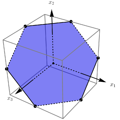
Figure 3: Graphical representation illustrating how the physical hexagonal support for the PDFs emerges by slicing the cube $|x_{i}|\leq 1$ ($i=1,2,3$) with the plane defined by the momentum conservation condition $x_{1}+x_{2}+x_{3}$.

A general observation is that QCD evolution equations enhance the region close to the origin and suppress the region close to the physical boundary. This suggests to use as the basic degrees of freedom to discretize the radius and angle on the $x_{1}+x_{2}+x_{3}=0$ surface, rather than the $x_{i}$ coordinates directly. In the given norm we can easily establish the notion of ‘angular-equispaced’ points. To build the intuition, we observe that in the standard Euclidean norm (that suggests a natural notion of angle) the angle between pairs of vectors is the same if their projections on the unit circle are equispaced. Extending this rule to our infinite norm we find that the ‘angles’ are equal if the points are equispace along the perimeter of the hexagon, that is generalization of the ‘circle’ for the norm (59).

This gives us a natural two dimensional space in terms of the radius and the angle in the infinite norm:

$$(x_{1},x_{2},x_{3})\equiv\bm{x}\to(r,\phi)$$ (60)

with

$$\begin{split}r(\bm{x})&=\max(|x_{1}|,|x_{2}|,|x_{3}|)\\ \phi(\bm{x})&=\begin{cases}\frac{x_{2}}{r},&\text{ for }x_{1}>0,x_{2}\geq 0,x_{3}<0,\\ \left(1-\frac{x_{1}}{r}\right),&\text{ for }x_{1}\leq 0,x_{2}>0,x_{3}<0,\\ \left(3-\frac{x_{2}}{r}\right),&\text{ for }x_{1}<0,x_{2}>0,x_{3}\geq 0,\\ \left(3-\frac{x_{2}}{r}\right),&\text{ for }x_{1}<0,x_{2}\leq 0,x_{3}>0,\\ \left(4+\frac{x_{1}}{r}\right),&\text{ for }x_{1}\geq 0,x_{2}<0,x_{3}>0,\\ \left(6+\frac{x_{2}}{r}\right),&\text{ for }x_{1}>0,x_{2}<0,x_{3}\leq 0,\\ \end{cases}\end{split}$$ (61)

such that $0<r\leqslant 1$ and $0\leqslant\phi<6$. The inverse map is

$$\bm{x}(r,\phi)=r\begin{cases}(1-\phi,\phi,-1)&0\leq\phi<1\\ (1-\phi,1,\phi-2)&1\leq\phi<2\\ (-1,3-\phi,\phi-2)&2\leq\phi<3\\ (-4+\phi,3-\phi,1)&3\leq\phi<4\\ (\phi-4,-1,5-\phi)&4\leq\phi<5\\ (1,\phi-6,5-\phi)&5\leq\phi<6\\ \end{cases}$$ (62)

This 2D space is suited for the discretization of the evolution problem, meaning that we set $\bm{x}(i,j)\equiv\bm{x}(\phi_{i},r_{j})$ for some choice of the grid points $\phi_{i},r_{j}$.

To be clear, a grid is a map from the sets of integers $[0,1,\cdots 6n-1]\times[0,1,\cdots,M]$ to the intervals $[0,6)\times[0,1]$ such that

$$(i,j)\to(\phi_{i},r_{j}).$$ (63)

For the angular variable the total number of points is such that each triangle that forms the hexagon has exactly $n$ points. To detail the features of the near-the-origin region, the radial grids should be chosen, in general, as non-linear functions. Due to the radial nature of evolution equation, it is simple to exclude the origin (or a small region near it) where typically there are no data and therefore no way to fix the distributions. Most grids in which the origin is excluded rely on some minimal value of $x$.

A desirable aspect of the radial grid is a high density near the origin, and a not too sparse density near the physical boundary. As a default option that has these characteristics we use an hyperbolic cosine map (a similar map is successfully used in artemide code [35, 36]). Specifically we use

$$r_{j}=\left[\text{cosh}\left(\frac{j-M}{Mc}\right)\right]^{-\alpha},\quad c^{-1}=-\text{acosh}\left(\frac{1}{x_{\text{\tiny min}}^{1/\alpha}}\right)$$ (64)

where $c$ is the constant that fixes $r_{0}=x_{\text{\tiny min}}$ and a typical good value for $\alpha$ is $3$. The inverse map is

$$j=M\left[1+c\ \text{acosh}\left(\frac{1}{r_{j}^{1/\alpha}}\right)\right]$$ (65)

For the angular grid, the first and easiest option to consider is equispaced points. This is realized simply by choosing

$$\phi_{i}=\frac{i\text{$\>$mod$\>$}n}{n}+\left[\frac{i}{n}\right],$$ (66)

where the square brackets indicate integer division. The inverse map is quite trivially

$$i=n\phi_{i}.$$ (67)

Other options that are available in the implementations are described in the appendix A.

Generalizing the equations (65) and (67) to continuous values of the radius and angle one obtains the two functions:

$$\mathfrak{r}(\bm{x}) =M\left[1+c\ \text{acosh}\left(\frac{1}{(r(\bm{x}))^{1/\alpha}}\right)\right]$$ (68)

$$\mathfrak{f}(\bm{x}) =n\phi(\bm{x}),$$ (69)

with the obvious properties

$$\mathfrak{f}(\bm{x}(i,j))\equiv\phi_{i},\quad\mathfrak{r}(\bm{x}(i,j))\equiv r_{j}.$$ (70)

In the following we refer to the space spanned by $\mathfrak{f},\mathfrak{r}$ as the grid-coordinate space.

3.2 Interpolation

Having fixed a class of grids and the maps that transform from physical space to grid-coordinate space, the next step towards building the discretization of the evolution problem is to fix an interpolation function on the chosen grid. In the present work, we operate only with piece-wise linear interpolations, due to their numerical simplicity. This choice, due to the high locality of the interpolating functions, produces sparse evolution kernels. The trade-off of this choice is that a sizable number of points is required to reach good interpolation accuracy. The generalization to a higher-order interpolations seems to be an involved problem due to the non-Euclidean nature of the grid. To this end, the interpolation accuracy is the main precision limitation of our approach, and the implementation of a more accurate interpolation could be a good point for future investigations.

The aim of the interpolation is to write a (generically well-behaved) function of $\bm{x}$ as

$$f(\bm{x})=\sum_{i=0}^{6n-1}\sum_{j=0}^{M}f_{ij}\mathcal{I}_{ij}(\bm{x}),\quad f_{ij}\equiv f(\bm{x}(i,j))$$ (71)

The weight functions $\mathcal{I}_{ij}(\bm{x})\equiv\mathcal{I}_{ij}(\mathfrak{f}(\bm{x}),\mathfrak{r}(\bm{x}))$ are piece-wise linear functions in the transformed coordinates $\mathfrak{f},\mathfrak{r}$, see eqn. (72). With our choice for $\mathfrak{r}(\bm{x})$ this implies that the weights $\mathcal{I}_{ij}(\bm{x})$ are non-linear functions of the physical momentum fractions $\bm{x}$.

To build a piece-wise linear weight function $\mathcal{I}_{ij}$ in the $\mathfrak{f},\mathfrak{r}$ variables it is sufficient to consider grid points with $i\pm 1,j\pm 1$ (understanding the periodic nature of the index $i$ and the restrictions in the index $j$). With these nine points (eight on the edge and the center point $i,j$), there is still freedom on how to construct the linear interpolation. Our choice is to define two different weight functions:

$$\mathcal{I}^{\pm}_{ij}(\bm{x})=\text{max}\bigg{[}0,1-\text{max}\Big{(}|\mathfrak{f}(\bm{x})-i|\ ,\ |\mathfrak{r}(\bm{x})-j|\ ,\ |\mp\mathfrak{f}(\bm{x})-\mathfrak{r}(\bm{x})\pm i+j|\Big{)}\bigg{]}$$ (72)

each of which uses a subset of six out of the eight neighbors of $(i,j)$. These functions are pyramids with a non-regular hexagonal base. In fig. 4 we show the graphical representations of these functions. In panel (a) we show the basis of the pyramids and in panel (b) the three-dimensional graph for $\mathcal{I}^{+}_{ij}$ (the graph for $\mathcal{I}^{-}_{ij}$ is similar). For instance, the piece of the $\mathcal{I}_{ij}^{+}$ weight function that has as base the triangle formed by the three grid points $(i,j),(i,j-1),(i+1,j-1)$ has the following explicit expression:

$$\mathcal{I}^{+}_{ij}(\bm{x})=\mathfrak{r}(\bm{x})-j+1\quad\text{ if }\mathfrak{f}(\bm{x})\geq i,\ \mathfrak{r}(\bm{x})>j-1,\ \mathfrak{f}(\bm{x})+\mathfrak{r}(\bm{x})<i+j$$ (73)

The base triangle is shaded in red in fig. 4. From this expression it is clear that if the point $(\mathfrak{f}(\bm{x}),\mathfrak{r}(\bm{x}))$ remains inside the triangle the weight function is linear.

[width=]Figures/two_grid

(a)

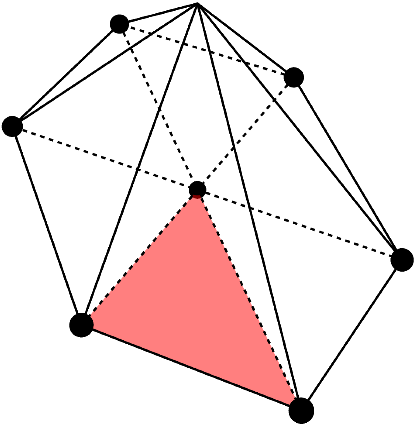
(b)

Figure 4: Panel (a) shows the subdivision in triangles of the basis of the two weight functions $\mathcal{I}^{\pm}_{ij}$. Panel (b) shows the 3D representation of the weight function $\mathcal{I}^{+}_{ij}$. The vertex of the pyramid has height equal to $1$. The red shaded triangle is used to guide with the orientation.

Using either solely $\mathcal{I}^{+}_{ij}$ or solely $\mathcal{I}^{-}_{ij}$ disturbs the symmetries of the task with respect to reflections, resulting into undesired artifacts in the solution. Thus, to preserve the natural symmetries and to reduce inaccuracies, we utilize the composition of both, and construct our interpolation as

$$f(\bm{x})=\sum_{i=0}^{6n-1}\sum_{j=0}^{M}f_{ij}\frac{\mathcal{I}^{+}_{ij}(\bm{x})+\mathcal{I}^{-}_{ij}(\bm{x})}{2}.$$ (74)

Finally, with the interpolation for a generic function defined, we can discretize the evolution kernels. The generic expression is

$$H_{i^{\prime}j^{\prime}}^{ij}=\frac{H_{i^{\prime}j^{\prime}}^{+,ij}+H_{i^{\prime}j^{\prime}}^{-,ij}}{2}=\frac{1}{2}\left(\mathbb{H}\mathcal{I}^{+}_{i^{\prime}j^{\prime}}(\bm{x}(i,j))+\mathbb{H}\mathcal{I}^{-}_{i^{\prime}j^{\prime}}(\bm{x}(i,j))\right).$$ (75)

The evolution equation for, e.g. the non-singlet, becomes

$$\mu^{2}\frac{\partial}{\partial\mu^{2}}\mathfrak{S}^{ij}_{\text{\tiny NS}_{i}}=-a_{s}(\mu^{2})\sum_{i^{\prime}=0}^{6n-1}\sum_{j^{\prime}=0}^{M}\left(H_{\text{\tiny NS}}\right)_{i^{\prime}j^{\prime}}^{ij}\mathfrak{S}^{i^{\prime}j^{\prime}}_{\text{\tiny NS}_{i}}$$ (76)

and similarly for the chiral-odd and the singlet cases.

We have found that a grid of size $60\times 15$ is sufficient for an average relative interpolation precision of $10^{-2}$, while $120\times 25$ provides precision $10^{-3}$. The highest uncertainty of reconstruction is concentrated at $r(\bm{x})\to 1$, if we exclude the outer part of hexagon ($r(\bm{x})<0.9$) the average interpolation precision became $\sim 10^{-4}$ (Note that in the physical case, the absolute values for the PDFs at $r(\bm{x})\to 1$ are small, and turn to zero at the boundary). These tests have been performed using the model in eq. (84). Comparing with other performed tests, we have concluded that the interpolation is the main source of numerical uncertainty in our code. In what follows we use grids $120\times 25$ for tests, and consider it as a default choice.

To determine the discretized kernels one has to carry out the defying integrals given in appendix B. The numerical evaluation is straightforward, once a few delicate points have been addressed. To highlight these points, we consider a part of $\widehat{\mathcal{H}}_{12}$ kernel. For the sake of shortness we denote $x_{1,2,3}^{ij}\equiv x_{1,2,3}(i,j)$ and focus on the action on the $\mathcal{I}^{+}$ function, since the same considerations apply to $\mathcal{I}^{-}$. The kernel is

$$\widehat{\mathcal{H}}_{12}\mathcal{I}^{+}_{i^{\prime}j^{\prime}}(\bm{x}^{ij})=\int_{-\infty}^{\infty}dv\frac{x^{ij}_{1}\Theta(x^{ij}_{1},-v)}{v(v-x^{ij}_{1})}\left[\mathcal{I}^{+}_{i^{\prime}j^{\prime}}(\bm{x}^{ij})-\mathcal{I}^{+}_{i^{\prime}j^{\prime}}(x_{1}^{ij}-v,x_{2}^{ij}+v,x_{3}^{ij})\right]$$ (77)

The first term in the square brackets performs the subtraction that makes the integral well-defined at $v=0$. The subtraction term has an integration range over the whole real line, while for other terms the integration range is limited by the support of $\mathcal{I}^{+}_{i^{\prime}j^{\prime}}$.

It can be directly checked that our choice for the weight functions satisfies

$$\mathcal{I}^{+}_{i^{\prime}j^{\prime}}(\bm{x}^{ij})=\delta_{ii^{\prime}}\delta_{jj^{\prime}}\mathcal{I}^{+}_{ij}(\bm{x}^{ij}),$$ (78)

which naturally leads to a decomposition of the kernel in a diagonal, proportional to $\delta_{ii^{\prime}}\delta_{jj^{\prime}}$ and a non-diagonal parts. Let us start with the latter, for which the subtraction constant is absent:

$$\int_{-\infty}^{\infty}dv\frac{x^{ij}_{1}\Theta(x^{ij}_{1},-v)}{v(x^{ij}_{1}-v)}\mathcal{I}^{+}_{i^{\prime}j^{\prime}}(x_{1}^{ij}-v,x_{2}^{ij}+v,x_{3}^{ij}).$$ (79)

This integral could be computed numerically as is. However, to increase the accuracy and speed of the evaluation, it is preferable to identify the limits of the integration as they are restricted by the support of the interpolant $\mathcal{I}^{+}_{i^{\prime}j^{\prime}}$. Due to the non-linear nature of the grid, determining the exact support can be cumbersome. Instead, we can easily find a (sometimes) slightly larger range $[v_{\text{\tiny min}},v_{\text{\tiny max}}]$ which is guaranteed to contain the support in $v$ and is of comparable size. Given these values we solve the simple system of equations

$$\begin{split}&x_{1}^{\text{\tiny min}}\leq x_{1}^{ij}-v\leq x_{1}^{\text{\tiny max}},\quad x_{2}^{\text{\tiny min}}\leq x_{2}^{ij}+v\leq x_{2}^{\text{\tiny max}},x_{3}^{\text{\tiny min}}\leq x_{3}\leq x_{3}^{\text{\tiny max}}\Rightarrow\\ &v_{\text{\tiny min}}=\text{max}\left(x_{1}^{ij}-x_{1}^{\text{\tiny max}},x_{2}^{\text{\tiny min}}-x_{2}^{ij}\right),\quad v_{\text{\tiny max}}=\text{min}\left(x_{1}^{ij}-x_{1}^{\text{\tiny min}},x_{2}^{\text{\tiny max}}-x_{2}^{ij}\right).\end{split}$$ (80)

We stress that the minimal and maximal values are computed from the $i^{\prime}j^{\prime}$ point, not the $i,j$ one. Consequently, the non-diagonal part of the kernel is

$$\begin{cases}\displaystyle\int_{v_{\text{\tiny min}}}^{v_{\text{\tiny max}}}dv\frac{x^{ij}_{1}\Theta(x^{ij}_{1},-v)}{v(x^{ij}_{1}-v)}\mathcal{I}^{+}_{i^{\prime}j^{\prime}}(x_{1}^{ij}-v,x_{2}^{ij}+v,x_{3}^{ij})&\text{ if }x_{3}^{ij}\in[x_{3}^{\text{\tiny min}},x_{3}^{\text{\tiny max}}],v_{\text{\tiny min}}<v_{\text{\tiny max}}\\ 0&\text{ otherwise }\end{cases}$$ (81)

The determination of $v_{\text{\tiny min,max}}$ is obviously the same for the diagonal part of the kernel, that can now be decomposed as

$$\int_{v_{\text{\tiny min}}}^{v_{\text{\tiny max}}}dv\frac{x^{ij}_{1}\Theta(x^{ij}_{1},-v)}{v(v-x^{ij}_{1})}\left[\mathcal{I}^{+}_{ij}(\bm{x}^{ij})-\mathcal{I}^{+}_{ij}(x_{1}^{ij}-v,x_{2}^{ij}+v,x_{3}^{ij})\right]$$

$$+\mathcal{I}^{+}_{ij}(\bm{x}^{ij})\left[\int_{-\infty}^{v_{\text{\tiny min}}}dv+\int_{v_{\text{\tiny max}}}^{\infty}dv\right]\frac{x^{ij}_{1}\Theta(x^{ij}_{1},-v)}{v(v-x^{ij}_{1})}.$$ (82)

The integrals in the second line can be computed analytically and give

$$\mathcal{I}^{+}_{ij}(\bm{x}^{ij})\left[\theta(x^{ij}_{1})\log\left(1-\frac{x^{ij}_{1}}{v_{\text{\tiny min}}}\right)+\theta(-x^{ij}_{1})\log\left(1-\frac{x^{ij}_{1}}{v_{\text{\tiny max}}}\right)\right],$$ (83)

where we incidentally notice that both logs vanish for $x^{ij}_{1}=0$. Therefore, the final expression for the kernel is

$$\widehat{\mathcal{H}}_{12}\mathcal{I}^{+}_{i^{\prime}j^{\prime}}(\bm{x}^{ij}) =\left(\widehat{H}_{12}\right)_{i^{\prime}j^{\prime}}^{+,ij}=\delta_{i\neq i^{\prime}\text{ or }j\neq j^{\prime}}\int_{v^{i^{\prime}j^{\prime}}_{\text{\tiny min}}}^{v^{i^{\prime}j^{\prime}}_{\text{\tiny max}}}dv\frac{x^{ij}_{1}\Theta(x^{ij}_{1},-v)}{v(x^{ij}_{1}-v)}\mathcal{I}^{+}_{i^{\prime}j^{\prime}}(x_{1}^{ij}-v,x_{2}^{ij}+v,x_{3}^{ij})$$

$$+\delta_{ii^{\prime}}\delta_{jj^{\prime}}\mathcal{I}^{+}_{ij}(\bm{x}^{ij})\left[\theta(x^{ij}_{1})\log\left(1-\frac{x^{ij}_{1}}{v^{ij}_{\text{\tiny min}}}\right)+\theta(-x^{ij}_{1})\log\left(1-\frac{x^{ij}_{1}}{v^{ij}_{\text{\tiny max}}}\right)\right]$$

$$+\delta_{ii^{\prime}}\delta_{jj^{\prime}}\int_{v^{ij}_{\text{\tiny min}}}^{v^{ij}_{\text{\tiny max}}}dv\frac{x^{ij}_{1}\Theta(x^{ij}_{1},-v)}{v(v-x^{ij}_{1})}\left[\mathcal{I}^{+}_{ij}(\bm{x}^{ij})-\mathcal{I}^{+}_{ij}(x_{1}^{ij}-v,x_{2}^{ij}+v,x_{3}^{ij})\right]$$

where we added the superscripts to $v_{\text{\tiny min,max}}$ to avoid any confusion on which are the values of $x_{\text{\tiny min,max}}$ used for their computation.

This procedure is to be carried out in identical fashion for the other part of $\widehat{\mathcal{H}}_{12}$ and for all other kernels. Note that the rank-four tables of evolution kernels are sparse (with typical density of non-zero entries of $\sim 10^{-3}-10^{-4}$), therefore, we use dedicated sparse algebra algorithms for storage and multiplication of these kernels. The kernels are computed during the initialization stage of the codes and internally stored. Initialization times vary based on how many computational cores are available, but typically using $\sim$ 10 cores the initialization can be expected to finish in about $1\sim 10$ minutes.

The codes require the initial state of PDFs, initial and final scales, and the function $\alpha_{s}(\mu)$. Then it discretizes the input function, and combines it into C-parity-definite functions with flavor-singlet and non-singlet combinations. Then each flavor combination is evolved using a fourth-order Runge-Kutta algorithm. Results are combined into the definite-flavor combinations and delivered to the user.

4 Example evaluation

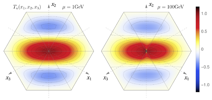
Figure 5: Evolution of the flavor-up distribution $T$ (4) from $1$ GeV to $100$ GeV. The boundary conditions are specified in eqn.(84).

4.1 Example of evolution

We have run and compared our codes in various circumstances, including stress tests (rapid functions, very dense grids, very small values of $x_{\text{min}}$, etc), and found a solid agreement between two independent implementations (both presented in the sec.5). The main source of numerical disagreement (of order of $\sim 10^{-7}$) is the differences in the implementation of the integral kernels, which is of the same order as the aimed numerical precision. If identical kernels are used, the agreement between implementations is of the order of $10^{-16}$.

Generally, we have observed that the evolution effects are not large in the bulk of the support of the function, but could result into significant changes of the functional form, especially in the vicinity of the origin. In this section, we demonstrate a simple example of results of evaluation.

One of the problems for the test is that a preferred physical form of twist-3 PDFs is unknown, since yet there are no phenomenological fits (the problem which is aimed by this project). Thus, for the demonstration, we have chosen a rather simple form of boundary condition:

$$\phi(x_{1,2,3}) =(1-x_{1}^{2})(1-x_{2}^{2})(1-x_{3}^{2})$$

$$T_{u}(x_{1,2,3}) =\cos(4x_{2})\phi(x_{1,2,3})\quad T_{d}(x_{1,2,3})=\left(2-\cos(3\pi\phi(x_{1,2,3}))\right)\phi(x_{1,2,3})$$

$$\Delta T_{u}(x_{1,2,3}) =\phi(x_{1,2,3})\left(\sin(\pi x_{2})+4(x_{1}^{2}-x_{3}^{2})\right)$$

$$\Delta T_{d}(x_{1,2,3}) =2\frac{\sin(\pi x_{2})}{\|\bm{x}\|_{\infty}}\left(1-\cos(\phi(x_{1,2,3}))\right)$$ (84)

$$T_{s}(x_{1,2,3}) =-\frac{3}{10}T_{d}(x_{1,2,3})\quad\Delta T_{s}(x_{1,2,3})=-\frac{3}{10}\Delta T_{d}(x_{1,2,3})$$

$$T^{+}(x_{1,2,3}) =\phi(x_{1,2,3})\|\bm{x}\|_{\infty}\sin(x_{1}-x_{3})\quad T^{-}(x_{1,2,3})=\phi(x_{1,2,3})\|\bm{x}\|_{\infty}\cos(x_{1}-x_{3})$$

These functions obey all required symmetries and turn to zero at $||\mathbf{x}||_{\infty}=1$. They are rather smooth at the origin, which could be (in)consistent with the physics.

To gauge the effect of evolution we present the $T_{u}$ distribution. In Fig.5 we show the boundary condition at a scale $\mu=1$ GeV on the left and the result of its evolution to $\mu=100$ GeV on the right. As one can see, the effect of evolution is not particularly pronounced at moderate values of $\|\bm{x}\|_{\infty}$. Most of the effect is concentrated for small values of $\|\bm{x}\|_{\infty}$, where the shape of distribution is modified. To have a clearer picture of the effects of evolution, in fig.6 we display two mono-dimensional sections of $T_{u}$. We show $T_{u}(-x,0,x)$ (which is the Qiu-Sterman function [33, 34]) on the left panel, and $T(x,-2x,x)$ on the right panel, which is the function along the line orthogonal to the Qiu-Sterman case (i.e. along the $x_{2}$ axis in Fig.5). We observe that the evolution has a strong effect in $\|\bm{x}\|_{\infty}\lesssim 10^{-1}$ region. This region is important in practice: for example, almost half of the data for the SIDIS transverse single-spin asymmetry, which is described by the distribution $T$, is measured at $\|\bm{x}\|_{\infty}\sim 0.1-0.05$ (see e.g. reviews of data in refs.[37, 38]), at scales from $\sim 1$GeV (for example [39]) till $\sim 90$GeV (for example [40]). However, specifically for the Qiu-Stermann $T_{u}(-x,0,x)$ the effect of the evolution is at most $10\%$, which can be considered negligible for many applications. From fig.6 it is also evident that it is essential to have a grid that manages the low $\|\bm{x}\|_{\infty}$ region accurately in order to achieve good accuracy for the evolution.

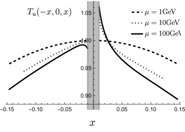
Figure 6: Comparison of two slices of $T_{u}$ when evolved from $1$ GeV to $100$ GeV: on the top $T_{u}(-x,0,x)$ with on the left the full range and on the right a zoomed-in version near the origin; on the bottom $T_{u}(x,-2x,x)$. The gray band displays the excluded region in $x$ due to the imposed constraint $x_{\text{min}}=10^{-2}$.

4.2 Comparison with the existing code of [17]

We have also compared against the code presented with the preprint [17] . In ref.[17] the discretization is realised with an equispaced grid in the variables $x_{1},x_{2}$. Albeit being a natural starting point, that we also employed in the first iteration of our implementation, it suffers from very low accuracy near $r(\bm{x})\sim 0$ point. We remind the reader, that this region is essential for the measurements at high energies. The problem can be partially mitigated by increasing the number of points in the grid. However, due to the scaling of the kernels as the fourth power of the number of points, this solution is not practical. Also, the kernel discretization in [17] was performed using the Simpson integration rule on the grid points, which greatly reduces the accuracy of the kernels with respect to the Gauss-Kronrod adaptive quadrature that we employ. Lastly, in ref.[17] the system of differential equations is solved by the direct exponentiation of the kernels, whereas our implementation is the 4th order Runge-Kutta algorithm, which has better precision.

Comparing the results of the test runs of our codes and the one of ref.[17] , we have found them generally compatible (especially for $r\gtrsim 0.2$, where both implementations have similar grid densities). The agreement however is still only in the $10\%$ range. For smaller values of $r$ the differences are larger. We have not found any bug or improper behavior in our implementations, which were independently written and cross-compared in the end. Therefore, we can only conclude that the approach of [17], albeit being in principle correct, suffers from large numerical inaccuracies.

5 Code interface

The two codes (C and FORTRAN) are to be separately compiled and are completely independent We strove for two different implementations with the same underlying logic in such a way that a cross-check between the implementations gives automatically a check of the implementations themselves. With the code is shipped a pre-computed set of kernels for $n=20$ and $M=25$, i.e. $120\times 25$ total points for the solution.

The codes are available at [1] for the C implementation and at [2] for the FORTRAN implementation. In the two following subsections we provide the necessary details to install and run the code. Please also refer to the tests files that are provided with each implementation for any further details.

5.1 C

The code, dubbed ‘honeycomb’ from the hexagonal support for the PDFs, is available at [1]. In the following, we present a description of how to interface with the library. More details and example evaluation can be found in the test files which are available in the tests/src directory.

To operate with the library the user must specify the input parameters and initialize the interface.

• The input parameters must be initialized first. This can be done directly in the code, or by reading a configuration card calling

  ⬇

  input_parameters_t *in_par =

  init_input_parameters(conf_path, to_save)

  where conf_path is the path to the configuration card and to_save is a boolean to control whether the configuration used should also be outputted to file.

• To initialize the interface itself the user must call

  ⬇

  evolution_interface_t *ei =

  init_evolution_interface(as, as_par,

  ev, in_par, v_l, ei, prev);

  where:

  • as and as_par are a function to compute $\alpha_{s}/4\pi$ and its parameters respectively.

  • ev is a pointer to an evolution_functions_t struct, which is a bundle of functions pointers to the relevant functions for the computation of the boundary conditions.

  • in_par is a pointer to the input_parameters_t struct.

  • v_l is a verbose level, which can be PL_NONE, PL_ESSENTIAL, PL_ALL.

  • ei is a pointer to an evolution_interface_t struct.

  • prev is a boolean that signals whether the previously stored state in the interface should be used as a starting point.

If the pointer to the evolution interface, which is passed as the argument, is set to NULL, then the interface is forced to perform complete initialization. Otherwise, if a valid pointer is given, the interface attempts to re-use a part of the information that is stored. If the interface is to be initialized, the boundary conditions are re-computed from the input functions no matter the value of the boolean passed as the last parameter to the initialization.

The review of the configuration options is given in appendix C. If any is left empty or given in the wrong format, the program will resort to default configuration for the problematic option. The order in which the parameters are given in the configuration card is irrelevant.

The evolution_functions_t fields follow the naming convention ${\tt Tf}\leftarrow T_{f}$, ${\tt DTf}\leftarrow\Delta T_{f}$ for the PDF of flavor $f$ and ${\tt TFp}\leftarrow T^{+}_{3F}$, ${\tt TFm}\leftarrow T^{-}_{3F}$ for the two gluon distributions. The parameter pointer is p_PDF. Important: the model must satisfy the physical symmetry relations (see sec. 2.1 and sec. 2.2), otherwise an incorrect result is obtained. During the initialization procedure of the evolution interface there is no automatic detection of the violation of the symmetries. To test the chosen model for violation of the symmetries one can use the check_*_symmetry functions, with ${\tt*}={\tt T,DT,TFp,TFm}$. These functions return either true (symmetry respected) or false (symmetry broken). If a point breaks the symmetries, its value is logged. The check is performed on a sample of $10^{4}$ random points inside the physical hexagon. If the $x_{\text{\tiny min}}$ value is invalid, the program is aborted.

To execute the evolution one can use either calls

⬇

saved_solution_t *solOut = execute_evolution(ei);

saved_solution_t **solOut_v = execute_evolution_w_steps(ei);

where the first one only saves the result at the final scale, whereas the second one saves the result at each step of the evolution. To export the solution to disk one can call

⬇

save_model(solOut, prefix, basis);

where prefix is a string that is prefixed to the filename and basis specifies the basis in which the solution is to be saved, valid options are the physical basis BASIS_PHYSICAL, the definite-C-parity basis BASIS_DEFINITE_C_PAR or both BASIS_BOTH. A previously computed model can be loaded via the load_model call.

Finally, to release the memory associated with the evolution interface, saved solution and input parameters, the user should make the calls

⬇

free_evolution_interface(&ei);

free_saved_solution(&solOut);

free_input_parameters(&in_par);

5.2 FORTRAN

The FORTRAN code has the name Snowflake, due to similarity of the twist-three support region with a snowflake (see fig.4(b)). The code is available at [2]. It is stand-alone and requires compiler FORTRAN 95 or newer. To compile the code one needs to update the compilator call in makefile (by default f95), and call make. The correctness of compilation can be checked by calling make test, which runs an elementary code and tests the proper linking between modules. The resulting object-files are stored in /obj. A simple single-files code can be compiled with Snowflake by calling make program TARGET=..., where dots are the path to the source code. An example of such a simple code can be found in /prog/EXAMPLE.f90.

The main module is snowflake, which contains several public functions and subroutines. The first subroutine to be called is

call Snowflake_Initialize(file,path)

Here, file is the name of INI-file, which contains all required setup information, and path is the optional argument with the path to the file (if path is absent the INI-file is searched in the directory of the program). The INI-file has specific format. The default configuration is presented in snowflake.ini in the root directory. The description of the INI-file is given in appendix D.

The initialization procedure allocates memory, and loads them from the storage, path to which is given in the INI-file. If the loading of kernels is switched off, the kernels will be computed. The latter can take significant time about 10-15 min for default configuration on a typical desktop. Kernels can be computed using the program prog/saveKernels.f90.

The computation of evolution is made by

call ComputeEvolution(mu0,mu1,alpha,G1,U1,D1,S1,C1,B1, G2,U2,D2,S2,C2,B2,inputQ,inputG)

where mu0 and mu1 are initial and final scales in GeV. alpha is a single-variable function which represents $\alpha_{s}(\mu)$. It has interface real*8:: alpha, mu. The arguments G1,U1,D1,S1,C1,B1,G2,U2,D2,S2,C2,B2 are optional, and represents two-variable functions f(x1,x2) with interfaces real*8::f,x1,x2. These functions are the boundary values for the evolved distribution at mu0. They are interpreted with accordance to optional parameters inputQ (accepts values ’T’, ’S’ or ’C’) and inputG (accepts values ’T’ or ’C’). The interpretation rules are

function	flag	interpretation	definition	symmetry
U1	inputQ=’T’	$T_{u}(x_{1},x_{2})$	(4,12,13)	(17)
U2	inputQ=’T’	$\Delta T_{u}(x_{1},x_{2})$	(5,12,13)	(17)
U1	inputQ=’S’	$S^{+}_{u}(x_{1},x_{2})$	(15)	(20)
U2	inputQ=’S’	$S^{-}_{u}(x_{1},x_{2})$	(16)	(20)
U1	inputQ=’C’	$\mathfrak{S}^{+}_{u}(x_{1},x_{2})$	(2.1)	(19)
U2	inputQ=’C’	$\mathfrak{S}^{-}_{u}(x_{1},x_{2})$	(2.1)	(19)
D1,D2,S1,S2,C1,C2,B1,B2 represent the boundary values of for $d$, $s$, $c$ and $b$ flavors correspondingly with the same interpretation rules.
G1	inputG=’T’	$T_{3F}^{+}(x_{1},x_{2})$	(24,26)	(30)
G2	inputG=’T’	$\Delta T_{3F}^{-}(x_{1},x_{2})$	(24,26)	(30)
G1	inputG=’C’	$\mathfrak{F}^{+}_{u}(x_{1},x_{2})$	(29)	(32)
G2	inputG=’C’	$\mathfrak{F}^{-}_{u}(x_{1},x_{2})$	(29)	(32)

If the argument is absent the corresponding boundary value is zero. The default values for flags are ’C’. The call of procedure evolves the boundary values to mu1 and stores in the memory.

Important: The boundary-value functions must satisfy the physical symmetry relations. Otherwise, the result of computation is incorrect. There is no internal check for consistency.

The value of the evolved function at $(x_{1},x_{2},-x_{1}-x_{2})$ can be obtained by call of the functions

real*8 GetPDF(x1,x2,f,outputT)

where x1 and x2 are real*8 variables $x_{1}$ and $x_{2}$. The integer f defines the type of the function with accordance to optional flag outputT (default value is ’C’). The type is selected with respect to the following table

f	n	-n	n	-n	n	-n	0 or 10	-10	0 or 10	-10
outputT=	’T’	’T’	’S’	’S’	’C’	’C’	’T’	’T’	’C’	’C’
return	$T_{q}$	$\Delta T_{q}$	$S^{+}_{q}$	$S^{-}_{q}$	$\mathfrak{S}^{+}_{q}$	$\mathfrak{S}^{-}_{q}$	$T_{3F}^{+}$	$T_{3F}^{-}$	$\mathfrak{F}^{+}$	$\mathfrak{F}^{-}$
n=1,2,3,4,5 and corresponds to quark flavors $d$, $u$, $s$, $c$, $b$, correspondingly.

To compute the evolution of functions $H$ or $E$ (6) call the subroutine

ComputeEvolutionChiralOdd(mu0,mu1,alpha,U1,D1,S1,C1,B1)

where mu0 and mu1 are initial and final scales in GeV. alpha is a single-variable function which represents $\alpha_{s}(\mu)$. The boundary conditions U1,D1,S1,C1,B1 are two-variable functions, which are interpreted as zero if absent. These functions are always interpreted as $H$ or $E$. Since $H$ and $E$ obey the same evolution equation, they are distinguished only by symmetries (18). The result at $(x_{1},x_{2})$ is invoked by

real*8 GetPDFChiralOdd(x1,x2,f)

where x1 and x2 are real*8 variables $x_{1}$ and $x_{2}$. The integer argument f=1,2,3,4,5 and corresponds to the flavors $d$, $u$, $s$, $c$, $b$, correspondingly. The type of output is dictated by the input, if the boundary values were symmetric (i.e. satisfy $H(x_{123})=H(-x_{321})$) the evolved function is $H$, and similar for function $E$. Note that the linearity of evolution equation implies that functions $H$ and $E$ can be evolved simultaneously, applying evolution to a general function those (anti-)symmetric part corresponds to $H$ ($E$).

6 Conclusions

This work presents an open-source, general purpose code for the evolution of twist-3 parton distribution functions (PDFs). The code is fully tested and could be easily integrated into other codes of a high-energy library. This is a prerequisite for a systematic analysis of structure functions that involves twist-3 PDFs. Various experimental measurements are sensitive to different projections of twist-3 PDFs, which are functions of two kinematic variables. Simultaneously, the total number of kinds of PDFs is not large: there are four types of quark and two types of gluon PDFs. Thus, a global analysis of variety of measurements can restrict these functions along various lines, while the evolution and loop corrections will relate these values to each other. Altogether, it opens the possibility for the first experimental determination of parton interference effects in the nucleon. The code-base presented in this work, provides one with tools to perform this analysis, giving the solutions for evolution, storage, discretization, and manipulations with twist-3 PDFs.

The paper also includes a review, in sec. 2, of the fundamental definitions and parametrizations of twist-3 PDFs. This translation dictionary can be used to relate various studies, since there is no standard choice of parametrization. This happens because there is no single definition for twist-3 objects that highlights all the relevant features. For instance, the evolution equations simplify dramatically in the definite C-parity basis, which is, however, quite unwieldy for perturbative computations of coefficient functions (see e.g.[12, 20]). In the same section we also provided an intuitive description of the geometry of the evolution equations, which is quite different compared to the standard twist-2 evolution, due to the two-dimensional support of the twist-3 PDFs.

The two-dimensional nature of the twist-3 PDFs requires adaptation and modification of the standard techniques that are well established for solving twist-2 evolution. In sec. 3 we provided ample explanation to the natural radial-angular coordinate system that we used to define a discretization of the problem. Such a coordinate system allows one to impose a higher density of grid points towards the physical origin, which is essential for future phenomenological applications. Moreover, the union of the coordinate system and choice of interpolation functions ensure that the radial ordering of the kernels, described in the sec. 2 is maintained in the discretized problem.

We decided to implement the evolution problem in two separate and independent codes. One is written in the FORTRAN language (and called snowflake), the other in the C language (and called honeycomb). This double implementation not only helps lowering the barrier to the usage of the codes in different projects, but also allowed us to cross-check implementations. The latter is important since the only another evolution code for twist-3 PDFs is available [17], and does not provide sufficient accuracy. Our implementation can be easily incorporated in larger existing projects and it is independent of any external library (except from libomp). The codes are available at [1] for the C implementation and at [2] for the FORTRAN implementation.

Appendix A Different grids

In this appendix, we present all types of grids that are currently implemented in the code. The grid along the radios and the angle can be specified independently, and thus presented independently. To select the type of the grid in the C-code, one must specify fields radial_grid_type, and angular_grid_type in the configuration file accordingly. To select the type of the grid in the Fortran-code, one must modify the compiler variables GRIDTYPE_R and GRIDTYPE_PHI at the beginning of the HexGrid.f90 file, and recompile the library.

The default option for the radial grid is given by the hyperbolic cosine map in eqn.(64).

The second option for the radial grid is the ‘log-exp’ type of grid, where

$$r_{j}=\exp\left[-\log(x_{\text{\tiny min}})\frac{j-M}{M}\right],\quad j\in[0,M],$$ (85)

being $x_{\text{\tiny min}}$ the minimal allowed value for the radius. This grid has the obvious feature that $r_{0}=x_{\text{\tiny min}}$. The inverse transformation is

$$j=M\left[1-\frac{\log(r(\bm{x}))}{\log(x_{\text{\tiny min}})}\right].$$ (86)

The third option of the radial grid is the ‘root-power’ type of grid, where we define

$$r_{j}=\left(\frac{\frac{j}{M}+c}{1+c}\right)^{\alpha}.$$ (87)

For the $j=M$ point grid reaches the maximum value $r_{M}=1$, automatically. The minimum value is defined by parameter $c$, which is fixed such that $r_{0}=x_{\text{\tiny min}}$. We find

$$c=\frac{x_{\text{\tiny min}}^{1/\alpha}}{1-x_{\text{\tiny min}}^{1/\alpha}}.$$ (88)

The inverse transformation is

$$j=M\left[(1+c)\left(r(\bm{x})\right)^{1/\alpha}-c\right].$$ (89)

The parameter $\alpha$ controls the distribution points. For $\alpha>1$, the points are denser at $x\to x_{\text{min}}$. The case for $\alpha=1$ represents the radial equispaced case.

One can see that the log-exp grid is very dense near the origin, and somewhat sparse near the physical boundary. The root-power grid is less dense near the origin and denser near the physical boundary (the exact behavior depends on the choice of $\alpha$, where $0<\alpha<1$ makes the grid sparse near the origin and should be avoided in practice). Ideally, we would keep the same density near the origin as the log-exp grid and have a grid with a comparable density as the root-power one with $\alpha\sim 2,3$ near the physical boundary. This can be achieved by modifying the log-exp grid and adding a second log. Specifically, we can take

$$r=2\frac{\exp\left[\frac{j-M}{Mc}\right]}{1+\exp\left[\frac{j-M}{Mc}\right]},$$ (90)

which inverts to

$$j=M\left[1+c\log\left(\frac{r}{2-r}\right)\right],\quad c^{-1}=-\log\left(\frac{x_{\text{\tiny min}}}{2-x_{\text{\tiny min}}}\right).$$ (91)

This grid exhibits the low-$x$ behavior of the log-exp grid and the large-$x$ behavior of the root-power grid.

To help the comparison between the different grids we show in fig. 7 the (continuous) map from $\mathfrak{r}$ to $r$ for each specific grid choice. The flatter a line in the plot is, the denser is the corresponding grid. It is evident how all the choices have comparable densities near the origin, but only the hyperbolic cosine map has also a satisfactory density near the physical border (which corresponds to the right-most part of the abscissa).

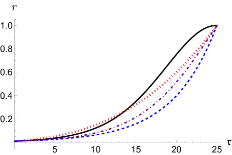
Figure 7: The solid black line is the hyperbolic cosine map of eqn.(64), the blue dashed line is the log-exp map of eqn.(85), the red dotted line is the root-power grid of eqn. (88), and the purple dot-dashed line is the double-log map of eqn. (90). All grid are showed using $x_{min}=10^{-2}$, $M=25$ and for the hyperbolic cosine and root-power grids the $\alpha$ exponent is fixed to $3$.

For the angular grids, an alternative to the equispaced points is a map that increases the density of points towards the lines $x_{1,2,3}=0$. For instance, one can use a cosine map:

$$\phi_{i}=\frac{1}{2}-\frac{1}{2}\cos\left(\pi\frac{i\text{$\>$mod$\>$}n}{n}\right)+\left[\frac{i}{n}\right]$$ (92)

with an inverse that is a bit more cumbersome than the simple linear map:

$$i=\left[\phi(\bm{x})\right]n+\frac{n}{\pi}\text{arccos}\left[1-2\text{$\>$mod$\>$}(\phi(\bm{x}),1)\right]$$ (93)

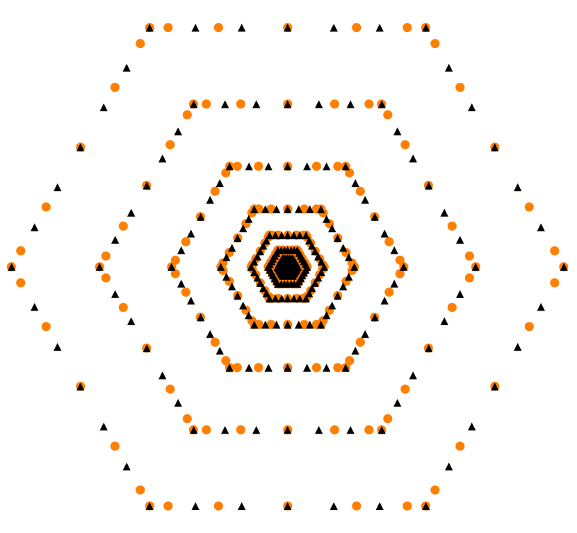
(a)

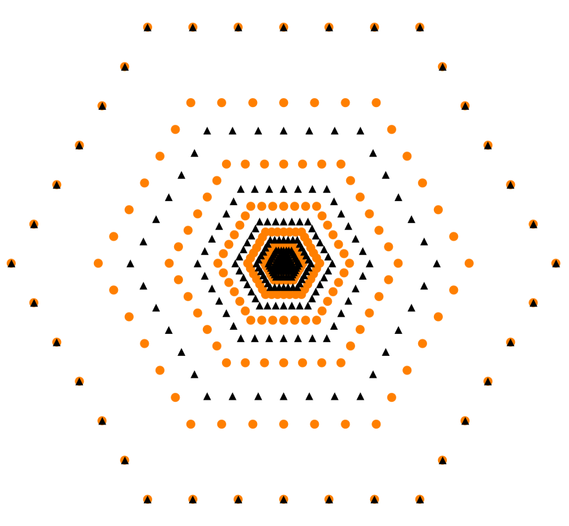
(b)

Figure 8: Panel (a) is the graphical representation of the grid with cosine angular scaling (orange dots) and linear angular scaling (black triangles) both using the double-log radial grid. Panel (b) is the graphical representation of the double-log grid (orange dots) and the single-log grid (black triangles) both using the linear angular grid

Appendix B Evolution kernels

In this appendix, we collect the expressions for the evolution kernels in momentum space. For their presentation, we use the notation

$$\Theta(a,b)\equiv\theta(a)\theta(b)-\theta(-a)\theta(-b)$$ (94)

where

$$\theta(a)=\begin{cases}1&a>0\\ 0&a\leq 0\end{cases}$$ (95)

The condition $\theta(0)=0$ secures the numerical stability of the implementation but introduces the necessity of treating the points $x_{i}=0$ (where $x_{i}$ is one of the generic momentum fractions) carefully. To isolate singular contributions we introduce the function

$$\delta_{x_{i},0}=\begin{cases}1&\text{ if }x_{i}=0,\\ 0&\text{ otherwise.}\end{cases}$$ (96)

We observe two different types of behaviors at $x_{i}=0$.

• First, the kernels are continuous and well-defined for $x_{i}=0$, but a direct numerical implementation would suffer from inaccuracies introduced by the cancellation of large contributions of different signs. This happens, for instance, in the $\mathcal{H}^{+}$ kernels. To provide accurate and reliable results we isolate the problematic point and compute the kernel separately. The isolation of the problematic point generates a structure of the form $\delta_{x_{i},0}(\cdots)+\delta_{x_{i}\neq 0}(\cdots)$.

• Second, the final expression for the kernel is ambiguous and the point $x_{i}=0$ cannot be straightforwardly isolated. This happens solely for the pieces of the $\widehat{\mathcal{H}}$ kernels when one of the $x_{i}$ is a gluon momentum fraction and for the exchange kernel $\mathcal{H}_{23}^{e,(1)}$. To reliably treat these points, we have re-derived the momentum-space expressions starting from the unambiguous position-space expression [26], explicitly considering $x_{i}=0$ case. The isolation of the problematic point generates a structure of the form $\delta_{x_{i},0}(\cdots)+(\cdots)$, where there is no $\delta_{x_{i}\neq 0}$ contribution.

The transformation from the expressions in ref.[26] to the one presented in the following is achieved by using the variable transformation $v_{i}=x_{l}-v$ $v_{j}=x_{k}+v$, where for the most of cases $x_{l}=x_{i}$, $x_{k}=x_{j}$, except for the kernels marked with ‘$-$’ and ‘$e$’, where $x_{l}=x_{j}$ and $x_{k}=x_{i}$. The latter identification also clarifies why such kernels are referred to as ‘exchange kernels’. After the transformation, the three-variable $\Theta$-functions of [26] can be reduced to two-variable $\Theta$-functions with a little algebra.

B.1 Non-singlet kernels

For the leading-color contributions we have

$$\widehat{\mathcal{H}}_{12}\mathfrak{S} =\delta_{x_{2},0}\mathfrak{S}(x_{1},0,x_{3})$$ (97)

$$+\int dv\Bigg{[}-\frac{x_{1}\Theta(x_{1},-v)}{v(x_{1}-v)}\left(\mathfrak{S}(x_{1},x_{2},x_{3})-\mathfrak{S}(x_{1}-v,x_{2}+v,x_{3})\right)$$

$$\quad\quad+\frac{x_{2}\Theta(x_{2},v)}{v(v+x_{2})}\left(\mathfrak{S}(x_{1},x_{2},x_{3})-\frac{x_{2}}{v+x_{2}}\mathfrak{S}(x_{1}-v,x_{2}+v,x_{3})\right)\Bigg{]}$$

$$\widehat{\mathcal{H}}_{23}\mathfrak{S} =\delta_{x_{2},0}\mathfrak{S}(x_{1},0,x_{3})$$ (98)

$$+\int dv\Bigg{[}-\frac{x_{3}\Theta(x_{3},-v)}{v(x_{3}-v)}\left(\mathfrak{S}(x_{1},x_{2},x_{3})-\mathfrak{S}(x_{1},x_{2}+v,x_{3}-v)\right)$$

$$\quad\quad+\frac{x_{2}\Theta(x_{2},v)}{v(v+x_{2})}\left(\mathfrak{S}(x_{1},x_{2},x_{3})-\frac{x_{2}}{v+x_{2}}\mathfrak{S}(x_{1},x_{2}+v,x_{3}-v)\right)\Bigg{]}$$

$$\mathcal{H}^{+}_{12}\mathfrak{S} =\delta_{x_{3},0}\int dv\Theta(x_{1},-v)\frac{v(v-2x_{1})}{2(x_{1}-v)^{3}}\mathfrak{S}(x_{1}-v,-x_{1}+v,0)$$ (99)

$$+\delta_{x_{3}\neq 0}\int dv\Bigg{[}\Theta(x_{2},v)\frac{x_{2}^{2}(x_{2}-x_{3}+v)}{2(x_{2}+v)^{2}x_{3}^{2}}$$

$$\phantom{+\delta_{x_{3}\neq 0}\int dv}+\Theta(x_{1},-v)\frac{x_{1}(x_{2}-x_{3})}{2(x_{1}-v)x_{3}^{2}}\Bigg{]}\mathfrak{S}(x_{1}-v,x_{2}+v,x_{3})$$

For the color-suppressed contributions we have

$$\widehat{\mathcal{H}}_{13}\mathfrak{S} =\int dv\left(\frac{x_{3}\Theta(x_{3},v)}{v(x_{3}+v)}-\frac{x_{1}\Theta(x_{1},-v)}{v(x_{1}-v)}\right)$$ (100)

$$\qquad\qquad\times\left(\mathfrak{S}(x_{1},x_{2},x_{3})-\mathfrak{S}(x_{1}-v,x_{2},x_{3}+v)\right)$$

$$\mathcal{H}^{+}_{13}\mathfrak{S} =\delta_{x_{2},0}\int dv\Theta(-x_{1},v)\frac{v}{(v-i)^{2}}\mathfrak{S}(x_{1}-v,0,-x_{1}+v)$$ (101)

$$+\delta_{x_{2}\neq 0}\int dv\Bigg{[}\frac{x_{1}}{x_{2}(v-x_{1})}\Theta(x_{1},-v)$$

$$\phantom{+\delta_{x_{2}\neq 0}\int dv}+\frac{-x_{3}}{x_{2}(x_{3}+v)}\Theta(x_{3},v)\Bigg{]}\mathfrak{S}(x_{1}-v,x_{2},x_{3}+v)$$

$$\mathcal{H}^{-}_{12}\mathfrak{S} =\delta_{x_{3},0}\int dv\Theta(x_{1},-v)\frac{v^{2}}{2(x_{1}-v)^{3}}\mathfrak{S}(-x_{1}+v,x_{1}-v,0)$$ (102)

$$+\delta_{x_{3}\neq 0}\int dv\Bigg{[}\Theta(x_{1},-v)\frac{x_{1}(2x_{2}(x_{1}-v)-x_{1}(x_{2}+v))}{2(x_{1}-v)^{2}x_{3}^{2}}$$

$$\phantom{+\delta_{x_{3}\neq 0}\int dv}+\Theta(x_{2},v)\frac{x_{2}^{2}}{2(v+x_{2})x_{3}^{2}}\Bigg{]}\mathfrak{S}(x_{2}+v,x_{1}-v,x_{3})$$

$$\mathcal{H}^{e,(1)}_{23}P_{23}\mathfrak{S} =\delta_{x_{3},0}\mathfrak{S}(x_{1},0,x_{2})+\int dv\frac{x_{3}}{(x_{3}-v)^{2}}\Theta(x_{3},-v)\mathfrak{S}(x_{1},x_{3}-v,x_{2}+v)$$ (103)

B.2 Chiral-odd kernels

Compared to the non-singlet chiral even case, only two new kernels appear

$$\mathcal{H}^{+}_{23}H =\delta_{x_{1}0}\int dv\Theta(x_{3},-v)\frac{v(v-2x_{3})}{2(x_{3}-v)^{3}}H(0,-x_{3}+v,x_{3}-v)$$ (104)

$$+\delta_{x_{1}\neq 0}\int dv\Bigg{[}\Theta(x_{2},v)\frac{x_{2}^{2}(x_{2}-x_{1}+v)}{2(x_{2}+v)^{2}x_{1}^{2}}$$

$$\qquad\qquad+\Theta(x_{3},-v)\frac{x_{3}(x_{2}-x_{1})}{2(x_{3}-v)x_{1}^{2}}\Bigg{]}H(x_{1},x_{2}+v,x_{3}-v)$$

$$\mathcal{H}^{-}_{23}H =\int dv\Bigg{[}\Theta(x_{3},-v)\frac{x_{3}(2x_{2}(x_{3}-v)-x_{3}(x_{2}+v))}{2(x_{3}-v)^{2}x_{1}^{2}}$$ (105)

$$\qquad\qquad+\Theta(x_{2},v)\frac{x_{2}^{2}}{2(v+x_{2})x_{1}^{2}}\Bigg{]}H(x_{1},x_{3}-v,x_{2}+v)$$

$$=\delta_{x_{1}0}\int dv\Theta(x_{3},-v)\Bigg{[}-\frac{v^{2}}{2\left(v-x_{3}\right)^{3}}\Bigg{]}H(0,x_{3}-v,-x_{3}+v)$$ (106)

$$+\delta_{x_{1}\neq 0}\int dv\Bigg{[}\Theta(x_{3},-v)\frac{x_{3}(2x_{2}(x_{3}-v)-x_{3}(x_{2}+v))}{2(x_{3}-v)^{2}x_{1}^{2}}$$

$$\qquad\qquad\qquad+\Theta(x_{2},v)\frac{x_{2}^{2}}{2(v+x_{2})x_{1}^{2}}\Bigg{]}H(x_{1},x_{3}-v,x_{2}+v)$$

B.3 Singlet kernels: diagonal terms

For the diagonal quark-quark case we only need one extra kernel compared to the non-singlet, which reads

$$\mathcal{H}^{d}_{13}\mathfrak{S}=-\Theta(x_{1},x_{3})\frac{x_{1}x_{3}}{x_{2}^{3}}\int dv\mathfrak{S}(x_{1}-v,x_{2},x_{3}+v)$$ (107)

For the diagonal gluon-gluon case we need similar kernels as for the non-singlet case, but modified to accommodate the different conformal spin of the particle

$$\widehat{\mathcal{H}}_{12}\mathfrak{S} =\delta_{x_{1}0}\mathfrak{S}(0,x_{2},x_{3})+\delta_{x_{2}0}\mathfrak{S}(x_{1},0,x_{3})$$ (108)

$$+\int dv\Bigg{[}-\frac{x_{1}\Theta(x_{1},-v)}{v(x_{1}-v)}\left(\mathfrak{S}(x_{1},x_{2},x_{3})-\frac{x_{1}}{x_{1}-v}\mathfrak{S}(x_{1}-v,x_{2}+v,x_{3})\right)$$

$$\qquad\qquad+\frac{x_{2}\Theta(x_{2},v)}{v(x_{2}+v)}\left(\mathfrak{S}(x_{1},x_{2},x_{3})-\frac{x_{2}}{x_{2}+v}\mathfrak{S}(x_{1}-v,x_{2}+v,x_{3})\right)\Bigg{]}$$

Quite evidently we have that

$$\widehat{\mathcal{H}}_{23}\mathfrak{S} =\delta_{x_{2}0}\mathfrak{S}(x_{1},0,x_{3})+\delta_{x_{3}0}\mathfrak{S}(x_{1},x_{2},0)$$ (109)

$$+\int dv\Bigg{[}-\frac{x_{2}\Theta(x_{2},-v)}{v(x_{2}-v)}\left(\mathfrak{S}(x_{1},x_{2},x_{3})-\frac{x_{2}}{x_{2}-v}\mathfrak{S}(x_{1},x_{2}-v,,x_{3}+v)\right)$$

$$\qquad\qquad+\frac{x_{3}\Theta(x_{3},v)}{v(x_{3}+v)}\left(\mathfrak{S}(x_{1},x_{2},x_{3})-\frac{x_{3}}{x_{3}+v}\mathfrak{S}(x_{1},x_{2}-v,x_{3}+v)\right)\Bigg{]}$$

and

$$\widehat{\mathcal{H}}_{31}\mathfrak{S} =\delta_{x_{1}0}\mathfrak{S}(0,x_{2},x_{3})+\delta_{x_{3}0}\mathfrak{S}(x_{1},x_{2},0)$$ (110)

$$+\int dv\Bigg{[}-\frac{x_{3}\Theta(x_{3},-v)}{v(x_{3}-v)}\left(\mathfrak{S}(x_{1},x_{2},x_{3})-\frac{x_{3}}{x_{3}-v}\mathfrak{S}(x_{1}+v,x_{2},,x_{3}-v)\right)$$

$$\qquad\qquad+\frac{x_{1}\Theta(x_{1},v)}{v(x_{1}+v)}\left(\mathfrak{S}(x_{1},x_{2},x_{3})-\frac{x_{1}}{x_{1}+v}\mathfrak{S}(x_{1}+v,x_{2},x_{3}-v)\right)\Bigg{]}$$

For the “$+$”-kernels we have

$$\mathcal{H}^{+}_{12}\mathfrak{S} =\delta_{x_{3}0}\int dv\Theta(x_{1},-v)\left[-\frac{v\left(-6vx_{1}+6x_{1}^{2}+v^{2}\right)}{6\left(v-x_{1}\right)^{4}}\right]\mathfrak{S}(x_{1}-v,-x_{1}+v,0)$$ (111)

$$+\delta_{x_{3}\neq 0}\int dv\Bigg{[}\Theta(x_{1},-v)\left(\frac{x_{1}^{2}\left(-v\left(x_{1}+3x_{2}\right)+8x_{1}x_{2}+3x_{1}^{2}+3x_{2}^{2}\right)}{6\left(x_{1}+x_{2}\right)^{3}\left(v-x_{1}\right)^{2}}\right)$$

$$\qquad\qquad+\Theta(x_{2},v)\left(\frac{x_{2}^{2}\left(x_{2}\left(8x_{1}+v\right)+3x_{1}\left(x_{1}+v\right)+3x_{2}^{2}\right)}{6\left(x_{1}+x_{2}\right)^{3}\left(x_{2}+v\right)^{2}}\right)\Bigg{]}$$

$$\qquad\qquad\qquad\times\mathfrak{S}(x_{1}-v,x_{2}+v,x_{3})$$

$$\widetilde{\mathcal{H}}^{+}_{12}\mathfrak{S} =\delta_{x_{3}0}\int dv\Theta(x_{1},-v)\left[-\frac{v^{3}}{6\left(v-x_{1}\right)^{4}}\right]\mathfrak{S}(x_{1}-v,-x_{1}+v,0)$$ (112)

$$+\delta_{x_{3}\neq 0}\int dv\Bigg{[}\Theta(x_{1},-v)\left(-\frac{x_{1}^{2}\left(v\left(x_{1}+3x_{2}\right)-2x_{1}x_{2}\right)}{6\left(x_{1}+x_{2}\right)^{3}\left(v-x_{1}\right)^{2}}\right)$$

$$\qquad\qquad+\Theta(x_{2},v)\left(\frac{x_{2}^{2}\left(v\left(3x_{1}+x_{2}\right)+2x_{1}x_{2}\right)}{6\left(x_{1}+x_{2}\right)^{3}\left(x_{2}+v\right)^{2}}\right)\Bigg{]}\mathfrak{S}(x_{1}-v,x_{2}+v,x_{3})$$

$$\mathcal{H}^{+}_{13}\mathfrak{S} =\delta_{x_{2}0}\int dv\Theta(x_{1},-v)\left[-\frac{v\left(-6vx_{1}+6x_{1}^{2}+v^{2}\right)}{6\left(v-x_{1}\right)^{4}}\right]\mathfrak{S}(x_{1}-v,0,-x_{1}+v)$$ (113)

$$+\delta_{x_{2}\neq 0}\int dv\Bigg{[}\Theta(x_{1},-v)\left(\frac{x_{1}^{2}\left(-v\left(x_{1}+3x_{3}\right)+8x_{1}x_{3}+3x_{1}^{2}+3x_{3}^{2}\right)}{6\left(x_{1}+x_{3}\right)^{3}\left(v-x_{1}\right)^{2}}\right)$$

$$\qquad\qquad+\Theta(x_{3},v)\left(\frac{x_{3}^{2}\left(x_{3}\left(8x_{1}+v\right)+3x_{1}\left(x_{1}+v\right)+3x_{3}^{2}\right)}{6\left(x_{1}+x_{3}\right)^{3}\left(x_{3}+v\right)^{2}}\right)\Bigg{]}$$

$$\qquad\qquad\qquad\times\mathfrak{S}(x_{1}-v,x_{2},x_{3}+v)$$

$$\widetilde{\mathcal{H}}^{+}_{13}\mathfrak{S} =\delta_{x_{2}0}\int dv\Theta(x_{1},-v)\left[-\frac{v^{3}}{6\left(v-x_{1}\right)^{4}}\right]\mathfrak{S}(x_{1}-v,0,-x_{1}+v)$$ (114)

$$+\delta_{x_{2}\neq 0}\int dv\Bigg{[}\Theta(x_{1},-v)\left(-\frac{x_{1}^{2}\left(v\left(x_{1}+3x_{3}\right)-2x_{1}x_{3}\right)}{6\left(x_{1}+x_{3}\right)^{3}\left(v-x_{1}\right)^{2}}\right)$$

$$\qquad\qquad+\Theta(x_{3},v)\left(\frac{x_{3}^{2}\left(v\left(3x_{1}+x_{3}\right)+2x_{1}x_{3}\right)}{6\left(x_{1}+x_{3}\right)^{3}\left(x_{3}+v\right)^{2}}\right)\Bigg{]}\mathfrak{S}(x_{1}-v,x_{2},x_{3}+v)$$

For the “$-$”-kernels we have the inversion as for the non-singlet case:

$$\mathcal{H}_{12}^{-}\mathfrak{S} =\delta_{x_{3}0}\Theta(x_{1},-v)\int dv\Bigg{[}-\frac{v^{3}}{6\left(v-x_{1}\right)^{4}}\Bigg{]}\mathfrak{S}(-x_{1}+v,x_{1}-v,0)$$ (115)

$$+\delta_{x_{3}\neq 0}\int dv\Bigg{[}\left(-\frac{x_{1}^{2}\left(v\left(x_{1}+3x_{2}\right)-2x_{1}x_{2}\right)}{6\left(x_{1}+x_{2}\right)^{3}\left(v-x_{1}\right)^{2}}\right)\Theta(x_{1},-v)$$

$$\qquad\qquad+\left(\frac{x_{2}^{2}\left(v\left(3x_{1}+x_{2}\right)+2x_{1}x_{2}\right)}{6\left(x_{1}+x_{2}\right)^{3}\left(x_{2}+v\right)^{2}}\right)\Theta(x_{2},v)\Bigg{]}\mathfrak{S}(x_{2}+v,x_{1}-v,x_{3})$$

$$\mathcal{H}_{13}^{-}\mathfrak{S} =\delta_{x_{2}0}\Theta(x_{1},-v)\int dv\Bigg{[}-\frac{v^{3}}{6\left(v-x_{1}\right)^{4}}\Bigg{]}\mathfrak{S}(-x_{1}+v,0,x_{1}-v)$$ (116)

$$+\delta_{x_{2}\neq 0}\int dv\Bigg{[}\left(-\frac{x_{1}^{2}\left(v\left(x_{1}+3x_{3}\right)-2x_{1}x_{3}\right)}{6\left(x_{1}+x_{3}\right)^{3}\left(v-x_{1}\right)^{2}}\right)\Theta(x_{1},-v)$$

$$\qquad\qquad+\left(\frac{x_{3}^{2}\left(v\left(3x_{1}+x_{3}\right)+2x_{1}x_{3}\right)}{6\left(x_{1}+x_{3}\right)^{3}\left(x_{3}+v\right)^{2}}\right)\Theta(x_{3},v)\Bigg{]}\mathfrak{S}(x_{3}+v,x_{2},x_{1}-v)$$

B.4 Singlet kernels: quark-gluon terms

For the two kernels $\mathcal{V}^{\pm}$ we have

$$\mathcal{V}_{13}^{+}\mathfrak{F} =\delta_{x_{2}0}\Theta(x_{1},-v)\int dv\left[\frac{x_{1}^{2}}{\left(v-x_{1}\right)^{4}}\right]\mathfrak{F}(x_{1}-v,0,-x_{1}+v)$$ (117)

$$+\delta_{x_{2}\neq 0}\int dv\Bigg{[}\Theta(x_{1},-v)\left(-\frac{x_{1}x_{3}\left(3x_{1}+x_{3}-2v\right)}{\left(x_{1}+x_{3}\right)^{3}\left(v-x_{1}\right)^{2}}\right)$$

$$\qquad\qquad+\Theta(x_{3},v)\left(\frac{x_{1}x_{3}\left(x_{1}+3x_{3}+2v\right)}{\left(x_{1}+x_{3}\right)^{3}\left(x_{3}+v\right)^{2}}\right)\Bigg{]}\mathfrak{F}(x_{1}-v,x_{2},x_{3}+v)$$

$$\mathcal{V}_{13}^{-}\mathfrak{F} =\delta_{x_{2}0}\Theta(x_{1},-v)\int dv\left[\frac{v^{2}}{\left(v-x_{1}\right)^{4}}\right]\mathfrak{F}(-x_{1}+v,0,x_{1}-v)$$ (118)

$$+\delta_{x_{2}\neq 0}\int dv\Bigg{[}\Theta(x_{1},-v)\left(\frac{x_{1}\left(-x_{1}x_{3}+x_{1}^{2}+2vx_{3}\right)}{\left(x_{1}+x_{3}\right)^{3}\left(v-x_{1}\right)^{2}}\right)$$

$$\qquad\qquad+\Theta(x_{3},v)\left(\frac{x_{3}\left(x_{3}\left(x_{1}-x_{3}\right)+2vx_{1}\right)}{\left(x_{1}+x_{3}\right)^{3}\left(x_{3}+v\right)^{2}}\right)\Bigg{]}\mathfrak{F}(x_{3}+v,x_{2},x_{1}-v)$$

B.5 Singlet kernels: gluon-quark terms

Here we give expressions for the un-permuted combinations. The action of the permutation operator $P_{23}$ exchanges $x_{2}\leftrightarrow x_{3}$. we have

$$\mathcal{W}^{+}\mathfrak{S} =-\frac{1}{2}\int dv\left[\Theta(x_{1},-v)-\Theta(x_{3},v)\right]\mathfrak{S}(x_{1}-v,x_{2},x_{3}+v)$$ (119)

$$\mathcal{W}^{-}\mathfrak{S} =\delta_{x_{2}0}\int dv\Theta(x_{1},-v)\left[\frac{v^{2}}{\left(v-x_{1}\right)^{2}}\right]\mathfrak{S}(-x_{1}+v,0,x_{1}-v)$$ (120)

$$+\delta_{x_{2}\neq 0}\int dv\Bigg{[}\Theta(x_{1},-v)\frac{2x_{1}^{2}+\left(x_{1}+x_{3}\right)\left(v-x_{1}\right)}{2\left(x_{1}+x_{3}\right)\left(v-x_{1}\right)}$$

$$\qquad\qquad+\Theta(x_{3},v)\frac{2x_{3}^{2}-\left(x_{1}+x_{3}\right)\left(x_{3}+v\right)}{2\left(x_{1}+x_{3}\right)\left(x_{3}+v\right)}\Bigg{]}\mathfrak{S}(x_{3}+v,x_{2},x_{1}-v)$$

$$\Delta\mathcal{W}\mathfrak{S} =\delta_{x_{3}\neq 0}\int dv\left[\Theta(x_{3},v)-\Theta(x_{1},x_{3})x_{1}^{2}\frac{3x_{3}+x_{1}}{(x_{1}+x_{3})^{3}}\right]\mathfrak{S}(x_{1}-v,x_{2},x_{3}+v)$$ (121)

$$-\delta_{x_{3}0}\int dv\Theta(x_{1},-v)\mathfrak{S}(x_{1}-v,x_{2},v)$$

Appendix C Configuration file for C implementation

The following options can be specified:

name	type	description
n	positive integer	number of points for the angular grid in one sector; default: $20$
M	positive integer	number of points for the radial grid; default: $25$
mu0_2	positive double	initial scale in GeV2; default: $1$ GeV2
muF_2	positive double	final scale in GeV2; default: $10$ GeV2
nstep	positive integer	number of Runge-Kutta steps; default: $100$
n_thread	positive integer	number of threads for kernel initialization; default: $1$
charm_THR	positive double	charm threshold in GeV2; default: $(1.27)^{2}=1.6129$ GeV2
bottom_THR	positive double	bottom threshold in GeV2; default: $(4.18)^{2}=17.4724$ GeV2
xmin	double $\in(0,1)$	$\text{min}\lVert\bm{x}\rVert_{\infty}$; default: $10^{-2}$
interpolant_type	string: IT_BOTH, IT_PLUS, IT_MINUS	whether to use the average of $\mathcal{I}^{\pm}$ or just $\mathcal{I}^{+}$ or $\mathcal{I}^{-}$ for the interpolation; default: IT_BOTH
radial_grid_type	string: {LOG, PWR, IML, HYP}_GRID	version of the radial grid; default: HYP_GRID
angular_grid_type	string: {LIN, COS}_GRID	which version of the angular grid to use; default: LIN_GRID
grid_exponent	positive double	exponent for the HYP and PWR grids; default: $3$
chiral_even_evolution	boolean	whether to evolve the chiral-even sector; default: true
chiral_odd_evolution	boolean	whether to evolve the chiral-odd sector; default: true
basefolder	string	root folder in which the ‘dat’ directory is searched; both relative and absolute paths are accepted; default: "../../"
kernel_subfolder	string	subfolder of ‘dat/kernels/’ where the kernels are searched; default: ""
result_subfolder	string	subfolder of ‘dat/results/’ where the results are to be stored; default: ""
integration_rule	string: GK_{21, 31, 41, 61}	which Gauss-Kronrod rule to use; default: GK_21
model	string	unused; default: ""

An empty option raises a warning and the corresponding value is fixed to the default. Each value cannot contain: white spaces, commas, colons, semi-colons, tabs or equal sign. If it does, a warning is printed that informs how the characters beyond the special character have been parsed into tokens. If the warning is printed, please check the configuration file. Moreover, # can be used for comments. A general valid entry in the configuration file (with * any number of the special characters above) is *n*10*#.

Appendix D Configuration file for FORTRAN implementation

The initialization parameters for the FORTRAN code are kept in the text files, which have a numbered lines. They are summarized in the following table

#	type	Description
0	logical	Flag to print information on the initialization process, and internal parameters.
1	integer	Number of nodes in the angular sector, i.e. $n$ in (63)
2	integer	Number of nodes in the along the radius, i.e. $M$ in (63)
3	real	Minimal radius included in the grid
4	real	Tolerance parameter used for zero estimation
5	real	Tolerance for integration
6	real	Maximal step of Runge-Kutta procedure (in $\ln(\mu)$)
7	integer	Maximal number of processors allowed to use
8	logical	Flag indicating that Chiral-Even kernels are to be used
9	logical	Flag indicating that Chiral-Odd kernels are to be used
10	logical	Flag indicating that singlet-part of evolution accounted (i.e. mixing between flavors)
11	real	Mass of charm threshold.
12	real	Mass of bottom threshold.
13	logical	Flag indicating that kernels are to be read from files.
14	string	Path to directory with kernels.

References

- \bibcommenthead
-
[1]
honeycomb.
https://github.com/QCDatHT/honeycomb
release v1.0: https://zenodo.org/doi/10.5281/zenodo.11102676 -
[2]
Snowflake.
https://github.com/VladimirovAlexey/Snowflake
release v1.0: https://doi.org/10.5281/zenodo.11070767. Accessed: 2024-04-26 - Gribov and Lipatov [1972] Gribov, V.N., Lipatov, L.N.: Deep inelastic e p scattering in perturbation theory. Sov. J. Nucl. Phys. 15, 438–450 (1972)
- Altarelli and Parisi [1977] Altarelli, G., Parisi, G.: Asymptotic Freedom in Parton Language. Nucl. Phys. B 126, 298–318 (1977) https://doi.org/10.1016/0550-3213(77)90384-4
- Anselmino et al. [1995] Anselmino, M., Efremov, A., Leader, E.: The Theory and phenomenology of polarized deep inelastic scattering. Phys. Rept. 261, 1–124 (1995) https://doi.org/10.1016/0370-1573(95)00011-5 arXiv:hep-ph/9501369. [Erratum: Phys.Rept. 281, 399–400 (1997)]
- Kodaira et al. [1995] Kodaira, J., Yasui, Y., Uematsu, T.: Spin structure function g2 (x, Q**2) and twist - three operators in QCD. Phys. Lett. B 344, 348–354 (1995) https://doi.org/10.1016/0370-2693(94)01550-V arXiv:hep-ph/9408354
- Ji et al. [2006a] Ji, X., Qiu, J.-W., Vogelsang, W., Yuan, F.: A Unified picture for single transverse-spin asymmetries in hard processes. Phys. Rev. Lett. 97, 082002 (2006) https://doi.org/10.1103/PhysRevLett.97.082002 arXiv:hep-ph/0602239
- Ji et al. [2006b] Ji, X., Qiu, J.-w., Vogelsang, W., Yuan, F.: Single Transverse-Spin Asymmetry in Drell-Yan Production at Large and Moderate Transverse Momentum. Phys. Rev. D 73, 094017 (2006) https://doi.org/10.1103/PhysRevD.73.094017 arXiv:hep-ph/0604023
- Scimemi and Vladimirov [2018] Scimemi, I., Vladimirov, A.: Matching of transverse momentum dependent distributions at twist-3. Eur. Phys. J. C 78(10), 802 (2018) https://doi.org/10.1140/epjc/s10052-018-6263-5 arXiv:1804.08148 [hep-ph]
- Rodini and Vladimirov [2022] Rodini, S., Vladimirov, A.: Definition and evolution of transverse momentum dependent distribution of twist-three. JHEP 08, 031 (2022) https://doi.org/10.1007/JHEP08(2022)031 arXiv:2204.03856 [hep-ph]. [Erratum: JHEP 12, 048 (2022)]
- Braun et al. [2021a] Braun, V.M., Ji, Y., Vladimirov, A.: QCD factorization for chiral-odd parton quasi- and pseudo-distributions. JHEP 10, 087 (2021) https://doi.org/10.1007/JHEP10(2021)087 arXiv:2108.03065 [hep-ph]
- Braun et al. [2021b] Braun, V.M., Ji, Y., Vladimirov, A.: QCD factorization for twist-three axial-vector parton quasidistributions. JHEP 05, 086 (2021) https://doi.org/10.1007/JHEP05(2021)086 arXiv:2103.12105 [hep-ph]
- Bukhvostov et al. [1985] Bukhvostov, A.P., Frolov, G.V., Lipatov, L.N., Kuraev, E.A.: Evolution equations for quasi-partonic operators. Nucl. Phys. B 258, 601–646 (1985) https://doi.org/10.1016/0550-3213(85)90628-5
- Balitsky and Braun [1989] Balitsky, I.I., Braun, V.M.: Evolution Equations for QCD String Operators. Nucl. Phys. B 311, 541–584 (1989) https://doi.org/10.1016/0550-3213(89)90168-5
- Abdul Khalek et al. [2022] Abdul Khalek, R., et al.: Science Requirements and Detector Concepts for the Electron-Ion Collider: EIC Yellow Report. Nucl. Phys. A 1026, 122447 (2022) https://doi.org/%****␣main.bbl␣Line␣275␣****10.1016/j.nuclphysa.2022.122447 arXiv:2103.05419 [physics.ins-det]
- Aidala et al. [2019] Aidala, C.A., et al.: The LHCSpin Project (2019) arXiv:1901.08002 [hep-ex]
- Pirnay [2013] Pirnay, B.M.: t3evol - Numerical Solution of Twist-three Evolution Equations (2013) arXiv:1307.1272 [hep-ph]
- Jaffe [1983] Jaffe, R.L.: Parton Distribution Functions for Twist Four. Nucl. Phys. B 229, 205–230 (1983) https://doi.org/10.1016/0550-3213(83)90361-9
- Scimemi et al. [2019] Scimemi, I., Tarasov, A., Vladimirov, A.: Collinear matching for Sivers function at next-to-leading order. JHEP 05, 125 (2019) https://doi.org/10.1007/JHEP05(2019)125 arXiv:1901.04519 [hep-ph]
- Rein et al. [2023] Rein, F., Rodini, S., Schäfer, A., Vladimirov, A.: Sivers, Boer-Mulders and worm-gear distributions at next-to-leading order. JHEP 01, 116 (2023) https://doi.org/10.1007/JHEP01(2023)116 arXiv:2209.00962 [hep-ph]
- Kang and Qiu [2009] Kang, Z.-B., Qiu, J.-W.: Evolution of twist-3 multi-parton correlation functions relevant to single transverse-spin asymmetry. Phys. Rev. D 79, 016003 (2009) https://doi.org/10.1103/PhysRevD.79.016003 arXiv:0811.3101 [hep-ph]
- Boer et al. [1998] Boer, D., Mulders, P.J., Teryaev, O.V.: Single spin asymmetries from a gluonic background in the Drell-Yan process. Phys. Rev. D 57, 3057–3064 (1998) https://doi.org/10.1103/PhysRevD.57.3057 arXiv:hep-ph/9710223
- Kanazawa and Koike [2000] Kanazawa, Y., Koike, Y.: Chiral odd contribution to single transverse spin asymmetry in hadronic pion production. Phys. Lett. B 478, 121–126 (2000) https://doi.org/10.1016/S0370-2693(00)00261-6 arXiv:hep-ph/0001021
- Boer et al. [2003] Boer, D., Mulders, P.J., Pijlman, F.: Universality of T odd effects in single spin and azimuthal asymmetries. Nucl. Phys. B 667, 201–241 (2003) https://doi.org/10.1016/S0550-3213(03)00527-3 arXiv:hep-ph/0303034
- Eguchi et al. [2007] Eguchi, H., Koike, Y., Tanaka, K.: Twist-3 Formalism for Single Transverse Spin Asymmetry Reexamined: Semi-Inclusive Deep Inelastic Scattering. Nucl. Phys. B 763, 198–227 (2007) https://doi.org/10.1016/j.nuclphysb.2006.11.016 arXiv:hep-ph/0610314
- Braun et al. [2009] Braun, V.M., Manashov, A.N., Pirnay, B.: Scale dependence of twist-three contributions to single spin asymmetries. Phys. Rev. D 80, 114002 (2009) https://doi.org/10.1103/PhysRevD.80.114002 arXiv:0909.3410 [hep-ph]. [Erratum: Phys.Rev.D 86, 119902 (2012)]
- Braun et al. [2001] Braun, V.M., Korchemsky, G.P., Manashov, A.N.: Gluon contribution to the structure function g(2)(x, Q**2). Nucl. Phys. B 597, 370–398 (2001) https://doi.org/10.1016/S0550-3213(00)00754-9 arXiv:hep-ph/0010128
- Beppu et al. [2010] Beppu, H., Koike, Y., Tanaka, K., Yoshida, S.: Contribution of Twist-3 Multi-Gluon Correlation Functions to Single Spin Asymmetry in Semi-Inclusive Deep Inelastic Scattering. Phys. Rev. D 82, 054005 (2010) https://doi.org/10.1103/PhysRevD.82.054005 arXiv:1007.2034 [hep-ph]
- Ji and Belitsky [2015] Ji, Y., Belitsky, A.V.: Renormalization of twist-four operators in light-cone gauge. Nucl. Phys. B 894, 161–222 (2015) https://doi.org/%****␣main.bbl␣Line␣500␣****10.1016/j.nuclphysb.2015.03.002 arXiv:1405.2828 [hep-ph]
- Braun et al. [2001] Braun, V.M., Korchemsky, G.P., Manashov, A.N.: Evolution equation for the structure function g(2) (x, Q**2). Nucl. Phys. B 603, 69–124 (2001) https://doi.org/10.1016/S0550-3213(01)00165-1 arXiv:hep-ph/0102313
- Collins and Tung [1986] Collins, J.C., Tung, W.-K.: Calculating Heavy Quark Distributions. Nucl. Phys. B 278, 934 (1986) https://doi.org/10.1016/0550-3213(86)90425-6
- Braun et al. [2010] Braun, V.M., Manashov, A.N., Rohrwild, J.: Renormalization of Twist-Four Operators in QCD. Nucl. Phys. B 826, 235–293 (2010) https://doi.org/10.1016/j.nuclphysb.2009.10.005 arXiv:0908.1684 [hep-ph]
- Qiu and Sterman [1991] Qiu, J.-w., Sterman, G.F.: Single transverse spin asymmetries. Phys. Rev. Lett. 67, 2264–2267 (1991) https://doi.org/10.1103/PhysRevLett.67.2264
- Qiu and Sterman [1992] Qiu, J.-w., Sterman, G.F.: Single transverse spin asymmetries in direct photon production. Nucl. Phys. B 378, 52–78 (1992) https://doi.org/10.1016/0550-3213(92)90003-T
- Scimemi and Vladimirov [2020] Scimemi, I., Vladimirov, A.: Non-perturbative structure of semi-inclusive deep-inelastic and Drell-Yan scattering at small transverse momentum. JHEP 06, 137 (2020) https://doi.org/10.1007/JHEP06(2020)137 arXiv:1912.06532 [hep-ph]
- Moos et al. [2023] Moos, V., Scimemi, I., Vladimirov, A., Zurita, P.: Extraction of unpolarized transverse momentum distributions from fit of Drell-Yan data at N4LL (2023) arXiv:2305.07473 [hep-ph]
- Bury et al. [2021] Bury, M., Prokudin, A., Vladimirov, A.: Extraction of the Sivers function from SIDIS, Drell-Yan, and boson production data with TMD evolution. JHEP 05, 151 (2021) https://doi.org/10.1007/JHEP05(2021)151 arXiv:2103.03270 [hep-ph]
- Horstmann et al. [2023] Horstmann, M., Schafer, A., Vladimirov, A.: Study of the worm-gear-T function g1T with semi-inclusive DIS data. Phys. Rev. D 107(3), 034016 (2023) https://doi.org/10.1103/PhysRevD.107.034016 arXiv:2210.07268 [hep-ph]
- Qian et al. [2011] Qian, X., et al.: Single Spin Asymmetries in Charged Pion Production from Semi-Inclusive Deep Inelastic Scattering on a Transversely Polarized 3He Target. Phys. Rev. Lett. 107, 072003 (2011) https://doi.org/10.1103/PhysRevLett.107.072003 arXiv:1106.0363 [nucl-ex]
- Adamczyk et al. [2016] Adamczyk, L., et al.: Measurement of the transverse single-spin asymmetry in at RHIC. Phys. Rev. Lett. 116(13), 132301 (2016) https://doi.org/10.1103/PhysRevLett.116.132301 arXiv:1511.06003 [nucl-ex]