Scaling of phase count in multicomponent liquids

Abstract

Mixtures with many components can segregate into coexisting phases, e.g., in biological cells and synthetic materials such as metallic glass. The interactions between components dictate what phases form in equilibrium, but quantifying this relationship has proven difficult. We derive scaling relations for the number of coexisting phases in multicomponent liquids with random interactions and compositions, which we verify numerically. Our results indicate that interactions only need to increase logarithmically with the number of components for the liquid to segregate into many phases. In contrast, a stability analysis of the homogeneous state predicts a power-law scaling. This discrepancy implies an enormous parameter regime where the number of coexisting phases exceeds the number of unstable modes, generalizing the nucleation and growth regime of binary mixtures to many components.

Phase separation of multicomponent mixture plays crucial roles in living systems and synthetic materials. In living system, like biological cells, phase separation enables biomolecular condensates, which involves thousands of different components [1, 2, 3, 4]. In synthetic materials, controlling phase separation is essential for engineering high-performance multicomponent materials, such as high-entropy alloys and metallic glasses [5, 6]. In all these cases, interactions between constituents control what phases form and which components they enrich.

Simple multicomponent mixtures are often studied using equilibrium thermodynamics of the seminal Flory-Huggins model [7, 8]. Whereas phase separation of binary mixtures is textbook material [9], higher component counts create fundamental challenges. In particular, many different phases can coexist [10], depending on the overall composition and the pairwise interactions between components [11, 12, 13]. The details are captured by the intricate geometry of the high-dimensional phase diagrams [14]. The geometry was already explored by direct simulation [15, 16, 17, 18] and by convexifying the free energy landscape [19], which are both limited to small component counts. Alternatively, analyzing the stability of the homogeneous state [20, 21, 22, 16, 23, 24] readily provides results for many components, but it is unlikely that this approach predicts actual coexisting phases.

In this letter, we derive scaling relations that faithfully predict the number of coexisting phases in mixtures with many components and random interactions. We test these relations using an improved numerical method based on the free energy minimization of an incompressible mixture, characterized by mean volume fractions ${\bar{\phi}}_{i}$ of its ${N_{\mathrm{c}}}$ components for $i=1,2,\ldots,{N_{\mathrm{c}}}$ with $\sum_{i}{\bar{\phi}}_{i}=1$. In the simplest case of homogeneous state, the equilibrium physics is governed by the Flory-Huggins free energy density

$$f(\{{\bar{\phi}}_{i}\})=\frac{1}{2}\sum_{i,j=1}^{N_{\mathrm{c}}}\chi_{ij}{\bar{\phi}}_{i}{\bar{\phi}}_{j}+\sum_{i=1}^{N_{\mathrm{c}}}{\bar{\phi}}_{i}\ln{\bar{\phi}}_{i}\;,$$ (1)

which combines pairwise interactions, quantified by the symmetric Flory matrix $\chi_{ij}=\chi_{ji}$ with $\chi_{ii}=0$, and translational entropy captured by the last term [7, 8]. For some choices of $\chi_{ij}$, the system can lower its free energy by splitting into multiple phases. We discuss this phase separation in the simple case of a thermodynamically large system where phases are homogeneous and their interfaces are negligible, so that equilibrium states minimize the average free energy density

$$\bar{f}=\sum_{p=1}^{{N_{\mathrm{p}}}}J_{p}f(\{\phi_{i}^{(p)}\})\;,$$ (2)

where phase $p$ is described by its composition $\phi_{i}^{(p)}$ and the relative volume $J_{p}$ obeying $\sum_{p}J_{p}=1$. Material conservation additionally implies ${\bar{\phi}}_{i}=\sum_{p=1}^{{N_{\mathrm{p}}}}J_{p}\phi_{i}^{(p)}$. Coexisting phases can in principle be obtained by minimizing $\bar{f}$ for given interaction matrices $\chi_{ij}$ and average volume fractions ${\bar{\phi}}_{i}$. However, these parameters are often not directly accessible in real systems. To circumvent this challenge, we instead treat $\chi_{ij}$ and ${\bar{\phi}}_{i}$ as random variables to make robust predictions for how they impact the average number of the coexisting phases, ${\bar{N}_{\mathrm{p}}}$. In particular, we draw the entries of the interaction matrix $\chi_{ij}$ for $i<j$ independently from the normal distribution $\mathcal{N}({\bar{\chi}},{\sigma_{\chi}})$, parametrized by the mean interaction ${\bar{\chi}}$ and the standard deviation ${\sigma_{\chi}}$.

To build intuition, we start with the special case of identical interactions ($\chi_{i\neq j}={\bar{\chi}}$, ${\sigma_{\chi}}=0$) and symmetric compositions (${\bar{\phi}}_{i}=1/{N_{\mathrm{c}}}$). We first check whether the homogeneous state is unstable, which marks the parameter region where phase separation is inevitable. Mathematically, this corresponds to the region where the Hessian matrix $H_{ij}=\partial^{2}f/\partial\phi_{i}\partial\phi_{j}$ is no longer positive definite, i.e., where at least one eigenvalue is negative. For ${\bar{\phi}}_{i}=1/{N_{\mathrm{c}}}$, this is the case when [25]

$${\bar{\chi}}>{N_{\mathrm{c}}}\;,$$ (3)

suggesting interactions need to scale with the components count ${N_{\mathrm{c}}}$ to destabilize the homogeneous state.

Equilibrium states can exhibit phase separation even when the homogeneous state is (locally) stable [26, 27]. To estimate the minimum interaction strength necessary for phase separation, we next consider ${N_{\mathrm{c}}}$ coexisting phases, each enriching a single component while diluting all other components by the same volume fraction $\phi_{*}^{({N_{\mathrm{c}}})}$, with $\phi_{*}^{({N_{\mathrm{c}}})}\approx e^{-{\bar{\chi}}}$ for ${\bar{\chi}}\gg\ln{N_{\mathrm{c}}}$ [25]. The free energy associated with this phase separated state is necessarily lower than the homogeneous state when [25]

$${\bar{\chi}}>\frac{2{N_{\mathrm{c}}}}{{N_{\mathrm{c}}}-1}\ln{N_{\mathrm{c}}}\;,$$ (4)

which provides a lower bound for the interaction strength above which phase separated states are favored. The relation indicates that interactions required for phase separation need to scale only logarithmically with the component count ${N_{\mathrm{c}}}$. A comparison with Eq. (3) suggests that the stability of the homogeneous state is a bad proxy for the phase separation behavior of multicomponent liquids.

Since phase separation of multi-component liquids not only depends on interactions but also composition [24], we next study the average behavior for all permissible volume fractions (${\bar{\phi}}_{i}\geq 0$, $\sum_{i}\bar{\phi}_{i}=1$), maintaining identical interactions ($\chi_{i\neq j}={\bar{\chi}}$, ${\sigma_{\chi}}=0$). In this case, we expect the number of coexisting phases, ${N_{\mathrm{p}}}$, to vary between ${N_{\mathrm{p}}}=1$ (homogeneous system) and ${N_{\mathrm{p}}}={N_{\mathrm{c}}}$ (maximum allowed by Gibb’s phase rule [28]). Similarly, the number of unstable modes of the homogeneous state, ${N_{\mathrm{u}}}$, will vary between ${N_{\mathrm{u}}}=0$ and ${N_{\mathrm{u}}}={N_{\mathrm{c}}}-1$, since only ${N_{\mathrm{c}}}-1$ variables are independent due to incompressibility. These two extreme scenarios suggest the relation ${N_{\mathrm{p}}}\sim{N_{\mathrm{u}}}+1$.

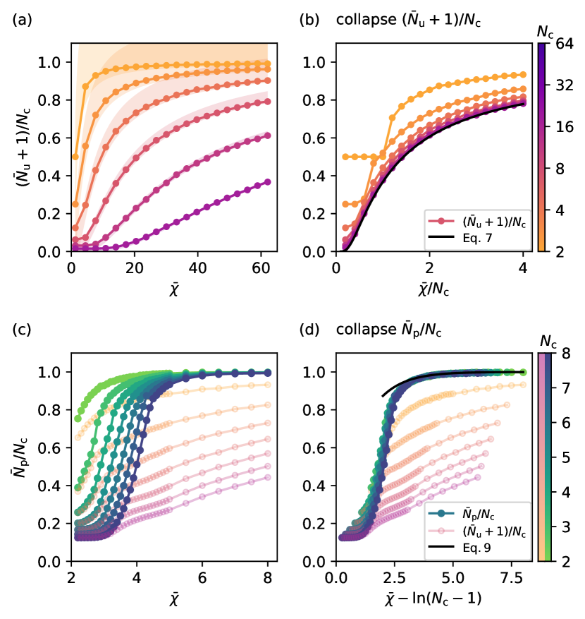
Figure 1: Average number of phases exceeds number of unstable modes for identical interactions. (a, b) Normalized average number of unstable modes, $({\bar{N}_{\mathrm{u}}}+1)/{N_{\mathrm{c}}}$, as a function of the mean interaction strength $\bar{\chi}$ in (a) and the scaled interaction $\bar{\chi}/{N_{\mathrm{c}}}$ in (b) for various component counts ${N_{\mathrm{c}}}$. The shaded area in (a) indicates the bounds given by Eq. (6), and the black line in (b) denotes the asymptotic expression (7). (c, d) Normalized average number of coexisting phases, ${\bar{N}_{\mathrm{p}}}/{N_{\mathrm{c}}}$, (green-blue) and $({\bar{N}_{\mathrm{u}}}+1)/{N_{\mathrm{c}}}$ (orange-purple) as a function of $\bar{\chi}$ in (c) and $\bar{\chi}-\ln({N_{\mathrm{c}}}-1)$ in (d). The black line in (d) marks the asymptotic expression (9). (a–d) Each dot results from an average over $500$–$20\,000$ uniformly sampled compositions.

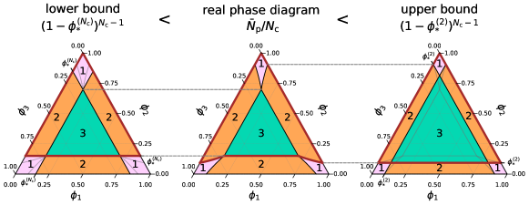
Figure 2: Illustration of phase count bounds. The center plot shows the phase diagram as a function of the volume fractions $\phi_{i}$ of ${N_{\mathrm{c}}}=3$ components for $\chi_{i\neq j}=2.8$. The colored regions indicate the number of coexisting phases, ${N_{\mathrm{p}}}=1,2,3$. The adjacent plots approximate the phase diagram using boundaries parallel to the axes, obtained by expanding the ${N_{\mathrm{p}}}=1$ region (left) or the central region with ${N_{\mathrm{p}}}={N_{\mathrm{c}}}$ (right). They respectively provide lower and upper bounds to the average phase count ${\bar{N}_{\mathrm{p}}}$, which can be obtained from the fraction covered by an area associated with each component (thick red lines).

To determine the average number of unstable modes, ${\bar{N}_{\mathrm{u}}}$, we chose random compositions using Beta distributions [11] and diagonalized the Hessian matrix $\boldsymbol{H}$ numerically. Fig. 1a shows that ${\bar{N}_{\mathrm{u}}}$ increases with the mean interaction strength $\bar{\chi}$, as expected. An analytical estimate for ${\bar{N}_{\mathrm{u}}}$ follows from Cauchy’s interlacing theorem: The number ${N_{\mathrm{u}}}$ of negative eigenvalues of $\boldsymbol{H}$ equals the number of sign changes in the sequence

$$\det{\boldsymbol{H}_{0}},\det{\boldsymbol{H}_{1}},\ldots,\det{\boldsymbol{H}_{{N_{\mathrm{c}}}-1}}\;,$$ (5)

where $\det{\boldsymbol{H}_{n}}=(\prod_{i=1}^{n}q_{i})(\sum_{i=1}^{n}q_{i}^{-1})$ is the determinant of the rank-$n$ leading minor of $\boldsymbol{H}$ with $q_{i}={\bar{\phi}}_{i}^{-1}-{\bar{\chi}}$ and $\det{\boldsymbol{H}_{0}}=1$. The number of sign changes in Eq. (5) is either $N_{-}$ or $N_{-}-1$, where $N_{-}$ is the number of negative $q_{i}$, i.e., the number of ${\bar{\phi}}_{i}$ larger than ${\bar{\chi}}^{-1}$ [25]. This implies that ${\bar{N}_{\mathrm{u}}}$ is bounded by $E_{{N_{\mathrm{c}}}}[{\bar{\phi}}_{i}>{\bar{\chi}}^{-1}]\leq{\bar{N}_{\mathrm{u}}}+1\leq E_{{N_{\mathrm{c}}}}[{\bar{\phi}}_{i}>{\bar{\chi}}^{-1}]+1$, where $E_{{N_{\mathrm{c}}}}[{\bar{\phi}}_{i}>h]={N_{\mathrm{c}}}(1-h)^{{N_{\mathrm{c}}}-1}$ denotes the expected number of ${\bar{\phi}}_{i}$ larger than $h$. The normalized average number of unstable modes, $({\bar{N}_{\mathrm{u}}}+1)/{N_{\mathrm{c}}}$, is thus bounded by

$$\left(1-\frac{1}{{\bar{\chi}}}\right)^{{N_{\mathrm{c}}}-1}\leq\frac{{\bar{N}_{\mathrm{u}}}+1}{{N_{\mathrm{c}}}}\leq\left(1-\frac{1}{{\bar{\chi}}}\right)^{{N_{\mathrm{c}}}-1}+\frac{1}{{N_{\mathrm{c}}}}\;,$$ (6)

consistent with our numerics; see Fig. 1a. The two bounds in Eq. (6) converge for large ${N_{\mathrm{c}}}$, implying

$$\frac{{\bar{N}_{\mathrm{u}}}+1}{{N_{\mathrm{c}}}}\overset{{N_{\mathrm{c}}}\gg 1}{\longrightarrow}\left(1-\frac{1}{{\bar{\chi}}}\right)^{{N_{\mathrm{c}}}-1}\overset{{\bar{\chi}}\gg 1}{\approx}e^{-{N_{\mathrm{c}}}/{\bar{\chi}}}\;.$$ (7)

This scaling indicates that the normalized number of unstable modes averaged over the phase diagram, ${\bar{N}_{\mathrm{u}}}/{N_{\mathrm{c}}}$, is controlled by the single scaled interaction parameter ${\bar{\chi}}/{N_{\mathrm{c}}}$. Fig. 1b shows that this scaling indeed collapses the numerical data for large ${N_{\mathrm{c}}}$, even for small $\bar{\chi}$.

To test how well the average number ${\bar{N}_{\mathrm{u}}}$ of unstable modes predicts the average phase count, ${\bar{N}_{\mathrm{p}}}$, we next investigate equilibrium states. In contrast to the unstable modes, it is difficult to obtain the coexisting states since they involve global information of the free energy landscape. To alleviate this challenge, we designed an efficient algorithm to determine coexisting states at arbitrary interactions and mean compositions, which is similar to the Gibbs ensemble method [29, 30, 31]. The method minimizes the mean free energy $\bar{f}$ given by Eq. (2) by redistributing components and volume across an ensemble of compartments, while obeying volume and material conservation [25]. In a key improvement over our earlier implementation [11, 10], we now initialize compartments such that the average fractions $\bar{\phi}_{i}$ can attain any value, which in principle allows us to determine the full $({N_{\mathrm{c}}}-1)$-dimensional phase diagram. Sampling the numerically obtained phase count ${N_{\mathrm{p}}}$ over the entire phase diagram allows us to estimate the average number of the coexisting phases in equilibrium, ${\bar{N}_{\mathrm{p}}}$.

The numerical results shown in Fig. 1c indicate that ${\bar{N}_{\mathrm{p}}}$ increases much more quickly with the interaction strength $\bar{\chi}$ than the number of unstable modes ${\bar{N}_{\mathrm{u}}}$. Moreover, the scaled interaction strength $\bar{\chi}/{N_{\mathrm{c}}}$, derived for ${\bar{N}_{\mathrm{u}}}$ from Eq. (7), cannot collapse these data. To derive an alternative scaling law, we focus on strong interactions, where Eq. (4) is satisfied, so we have the maximal number of phases (${N_{\mathrm{p}}}={N_{\mathrm{c}}}$) for equal composition at the center of the phase diagram ($\bar{\phi}_{i}=1/{N_{\mathrm{c}}}$). The region where these ${N_{\mathrm{c}}}$ phases are stable forms a $({N_{\mathrm{c}}}-1)$-dimensional simplex (green region in Fig. 2), which covers a larger area for higher ${\bar{\chi}}$. However, averaging ${N_{\mathrm{p}}}$ over the entire phase diagram is difficult since phase boundaries are generally curved. Instead, we next derive lower and upper bounds of ${\bar{N}_{\mathrm{p}}}$ by replacing curved boundaries with flat hyperplanes that are parallel to the axes of the phase diagram [25]. For the lower bound, we enlarge regions with few phases so their boundaries extend the flat boundaries of the central region, intersecting the axes at $\phi_{*}^{({N_{\mathrm{c}}})}$ (left plot in Fig. 2). For the upper bound, we move the straight boundaries of the central region such that their extensions intersect the axes of the phase diagram at $\phi_{*}^{(2)}$, which marks the coexistence point between the $1$-phase and $2$-phase region (right plot in Fig. 2). For both bounds, all phase boundaries are then parallel to the axes of the phase diagram, and the average phase count ${\bar{N}_{\mathrm{p}}}$ can be calculated from the volume of the smallest simplex enclosing the central region and one corner of the phase diagram. One of these simplexes is marked by the red line in Fig. 2, and there are two congruent regions anchored at the remaining corners. Since the phase count at each point in the phase diagram is given by the number of these simplexes covering that point, ${\bar{N}_{\mathrm{p}}}$ is simply ${N_{\mathrm{c}}}$ times the fraction covered by a single simplex. For general component counts, the normalized average phase count ${\bar{N}_{\mathrm{p}}}/{N_{\mathrm{c}}}$ is then bounded by [25]

$$\left(1-\phi_{*}^{({N_{\mathrm{c}}})}\right)^{{N_{\mathrm{c}}}-1}\leq\frac{{\bar{N}_{\mathrm{p}}}}{{N_{\mathrm{c}}}}\leq\left(1-\phi_{*}^{(2)}\right)^{{N_{\mathrm{c}}}-1}\;,$$ (8)

For ${\bar{\chi}}\gg 1$, the fractions $\phi_{*}^{({N_{\mathrm{c}}})}$ and $\phi_{*}^{(2)}$ converge to $e^{-{\bar{\chi}}}$, implying [25]

$$\frac{{\bar{N}_{\mathrm{p}}}}{{N_{\mathrm{c}}}}\overset{{\bar{\chi}}\gg 1}{\longrightarrow}\left(1-e^{-{\bar{\chi}}}\right)^{{N_{\mathrm{c}}}-1}\approx\exp\!\left[({N_{\mathrm{c}}}-1)e^{-{\bar{\chi}}}\right]\;.$$ (9)

This approximation reveals that ${\bar{N}_{\mathrm{p}}}$ is asymptotically given by $E_{{N_{\mathrm{c}}}}[{\bar{\phi}}_{i}>e^{-{\bar{\chi}}}]$, i.e., the expected number of ${\bar{\phi}}_{i}$ larger than $e^{-{\bar{\chi}}}$. This result is similar to that for ${\bar{N}_{\mathrm{u}}}$ following from Eq. (7), except the threshold is now $e^{-{\bar{\chi}}}$ instead of ${\bar{\chi}}^{-1}$. Consequently, we predict that ${\bar{N}_{\mathrm{p}}}/{N_{\mathrm{c}}}$ is controlled by the single shifted interaction parameter ${\bar{\chi}}-\ln({N_{\mathrm{c}}}-1)$. Indeed, Fig. 1d shows that this scaling collapses the data in a surprisingly large parameter range, even when the limits used in Eq. (9) are violated.

The data collapse that we identify in Fig. 1d indicates that the interaction parameter $\chi_{i\neq j}={\bar{\chi}}$ needs to exceed roughly $3+\ln({N_{\mathrm{c}}}-1)$ to have many phases (${\bar{N}_{\mathrm{p}}}\approx{N_{\mathrm{c}}}$). Since the stability analysis instead predicts a linear scaling of ${\bar{\chi}}$ with ${N_{\mathrm{c}}}$, we conclude that stability analysis is not suited to predict phase counts when components exhibit identical interactions.

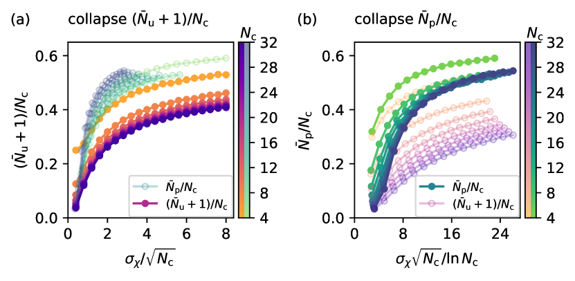
Figure 3: More variable random interactions imply more phases. Normalized average number of unstable modes, $({\bar{N}_{\mathrm{u}}}+1)/{N_{\mathrm{c}}}$ (orange-purple), and normalized average number of coexisting phases, ${\bar{N}_{\mathrm{p}}}/{N_{\mathrm{c}}}$ (green-blue), as a function of two different scalings of the standard deviation $\sigma_{\chi}$ of the interactions for various component counts ${N_{\mathrm{c}}}$ and ${\bar{\chi}}=0$. Each dot results from an average over $10^{3}$–$10^{4}$ pairs of random interaction matrices $\chi_{ij}$ and compositions ${\bar{\phi}}_{i}$.

We next extend our results by varying the individual interactions as well as the composition. For simplicity, we first consider vanishing mean interactions (${\bar{\chi}}=0$) and instead vary the standard deviation ${\sigma_{\chi}}$ of the normal distribution governing the symmetric interaction matrix $\chi_{ij}$. In the case of equal composition (${\bar{\phi}}_{i}={N_{\mathrm{c}}}^{-1}$), ${\bar{N}_{\mathrm{u}}}$ can be obtained from the eigenvalues of the random interaction matrix, which are distributed according to Wigner’s semicircle law and scale with $\sigma_{\chi}\sqrt{{N_{\mathrm{c}}}}$ [20]. The same scaling applies to the case of uniformly distributed compositions [25], suggesting that the normalized number of unstable modes, $({\bar{N}_{\mathrm{u}}}+1)/{N_{\mathrm{c}}}$, is controlled by $\sigma_{\chi}/\sqrt{{N_{\mathrm{c}}}}$ [20, 24]. Fig. 3a shows that this scaling can indeed collapse data for ${\bar{N}_{\mathrm{u}}}$, whereas it fails for the phase counts that we determined using our numerical algorithm.

To obtain a scaling for phase count, we recall the asymptotic scalings of ${\bar{N}_{\mathrm{u}}}$ and ${\bar{N}_{\mathrm{p}}}$ followed from expectation values involving the compositions and mean interaction strength ${\bar{\chi}}$, ${\bar{N}_{\mathrm{u}}}+1\sim E_{{N_{\mathrm{c}}}}[{\bar{\phi}}_{i}^{-1}<{\bar{\chi}}]$ and ${\bar{N}_{\mathrm{p}}}\sim E_{{N_{\mathrm{c}}}}[{\bar{\phi}}_{i}^{-1}<e^{{\bar{\chi}}}]$. These scalings suggest that interaction strengths related to unstable modes enter exponentially in similar expressions for the phase count. Specifically, this idea indicates that the normalized phase count ${\bar{N}_{\mathrm{p}}}/{N_{\mathrm{c}}}$ is controlled by the scaling parameter $\sigma_{\chi}\sqrt{{N_{\mathrm{c}}}}/\ln{{N_{\mathrm{c}}}}$ for random interaction matrices with vanishing mean (${\bar{\chi}}=0$) [25]. Indeed, Fig. 3b reveals that this scaling collapses ${\bar{N}_{\mathrm{p}}}/{N_{\mathrm{c}}}$ for sufficiently large ${N_{\mathrm{c}}}$. Thus, larger variations of the interactions lead to more phases, and ${\bar{N}_{\mathrm{p}}}/{N_{\mathrm{c}}}$ grows with ${N_{\mathrm{c}}}$ even when $\sigma_{\chi}$ is fixed. In contrast, stability analysis suggests that $\sigma_{\chi}$ needs to grow with $\sqrt{{N_{\mathrm{c}}}}$ to have the same fraction of unstable modes, so ${\bar{N}_{\mathrm{u}}}$ severely underestimates the phase count ${\bar{N}_{\mathrm{p}}}$, particularly for large ${N_{\mathrm{c}}}$.

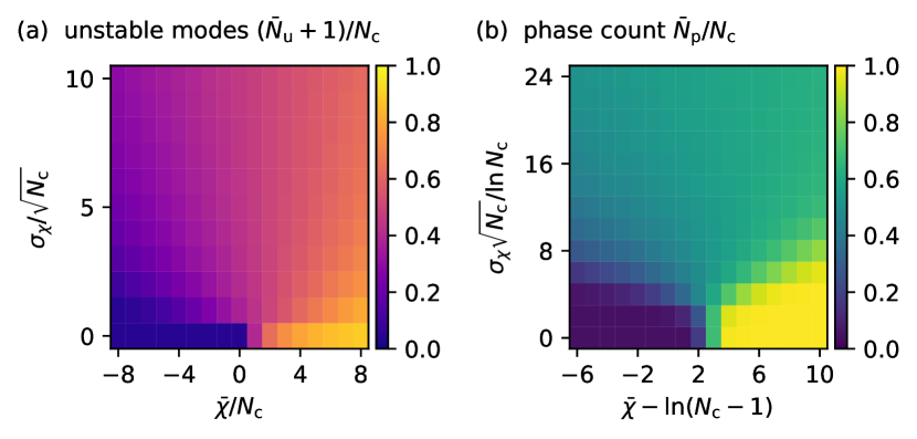
Figure 4: Numerically estimated master functions for Eqs. (10). (a) Normalized average number of unstable modes, $({\bar{N}_{\mathrm{u}}}+1)/{N_{\mathrm{c}}}$, as a function of scaled mean interaction ${\bar{\chi}}$ and standard deviation ${\sigma_{\chi}}$. (b) Normalized average number of coexisting phases, ${\bar{N}_{\mathrm{p}}}/{N_{\mathrm{c}}}$, as a function of scaled ${\bar{\chi}}$ and ${\sigma_{\chi}}$. (a, b) Functions were obtained by averaging $300$ samples of random interaction matrices and compositions for each value of ${\bar{\chi}}$ and ${\sigma_{\chi}}$ for component counts ${N_{\mathrm{c}}}=16,20,24,28,32$; see [25].

So far, we have identified how ${\bar{N}_{\mathrm{u}}}$ and ${\bar{N}_{\mathrm{p}}}$ scale with the component count ${N_{\mathrm{c}}}$ when interactions are identical (${\sigma_{\chi}}=0$) or their mean vanishes (${\bar{\chi}}=0$). To test whether these scalings persist when both ${\sigma_{\chi}}$ and ${\bar{\chi}}$ are nonzero, we next combine the control parameters derived for ${\sigma_{\chi}}=0$ (see Fig. 1) and for ${\bar{\chi}}=0$ (see Fig. 3) and postulate

$$\frac{{\bar{N}_{\mathrm{u}}}+1}{{N_{\mathrm{c}}}} \approx g_{\mathrm{u}}\left(\frac{{\bar{\chi}}}{{N_{\mathrm{c}}}},\;\frac{{\sigma_{\chi}}}{\sqrt{{N_{\mathrm{c}}}}}\right)\qquad\text{and}$$ (10a)

$$\frac{{\bar{N}_{\mathrm{p}}}}{{N_{\mathrm{c}}}} \approx g_{\mathrm{p}}\left({\bar{\chi}}-\ln({N_{\mathrm{c}}}-1),\;\frac{{\sigma_{\chi}}\sqrt{{N_{\mathrm{c}}}}}{\ln{{N_{\mathrm{c}}}}}\right),$$ (10b)

where $g_{\mathrm{u}}$ and $g_{\mathrm{p}}$ are master functions for the number of unstable modes and coexisting phases, respectively. We determine these functions by sampling random interaction matrices and random compositions for several components counts ${N_{\mathrm{c}}}$; see Fig. 4. Fig. A2 [25] shows that the deviation of the prediction of Eqs. (10) to the actually measured ${\bar{N}_{\mathrm{u}}}$ and ${\bar{N}_{\mathrm{p}}}$ is low in most parameter regions, implying that the proposed scaling captures the essence for different ${N_{\mathrm{c}}}$. Fig. 4 shows that both master functions are qualitatively similar: They are close to $0$ for strongly attractive interactions (large negative ${\bar{\chi}}$ and small ${\sigma_{\chi}}$) and they converge to $1$ when repulsive interactions dominate (large ${\bar{\chi}}$ and small ${\sigma_{\chi}}$), implying ${N_{\mathrm{c}}}$ coexisting phases. In contrast, both master functions predict $\frac{1}{2}{N_{\mathrm{c}}}$ for strongly varying interactions (small ${\bar{\chi}}$ and large ${\sigma_{\chi}}$), and the respective influence of ${\bar{\chi}}$ can be approximated analytically [25]. While the master functions exhibit similarities, the axes are scaled very differently, implying different interpretations of what constitutes large interactions: For large ${N_{\mathrm{c}}}$, the mean interactions ${\bar{\chi}}$ and the variance $\sigma_{\chi}^{2}$ need to scale with ${N_{\mathrm{c}}}$ to obtain similar fractions $g_{\mathrm{u}}$ of unstable modes. In contrast, the predictions for the phase count implies a much weaker dependence on ${N_{\mathrm{c}}}$.

Our results indicate that the interactions necessary to have large phase counts scale weakly with the component count ${N_{\mathrm{c}}}$. Consequently, even moderate interaction strengths of a few $k_{\mathrm{B}}T$ could lead to many coexisting phases, even for thousands of components, like in biological cells. In contrast, large ${N_{\mathrm{c}}}$ stabilizes the homogeneous state and much stronger interactions are necessary to have many unstable modes. On the one hand, this suggests that linear stability analysis is inadequate to investigate multiphase coexistence. On the other hand, the result implies that such multicomponent systems have an enormous parameter regime where multiple states are locally stable, enabling controlled transitions. For instance, biological cells could use active processes to form or dissolve droplets by crossing thermodynamic barriers [27]. To answer such questions and engineer such systems, a detailed understanding of the geometry of phase space, preferably for realistic interactions (e.g. including higher-order interactions [32]), would be helpful. Our scaling relations, and particularly the numerical method to determine coexisting phases, will guide future research in this direction.

The source code for this article is openly available from github XXX.

Appendix A Hessian of the free energy of homogeneous states

The stability of the homogeneous state is given by the eigenvalues of the Hessian of the free energy in Eq. (1),

$$\frac{\partial^{2}f}{\partial\phi_{i}\partial\phi_{j}}=\chi_{ij}+\frac{\delta_{ij}}{\phi_{i}}-\chi_{1j}-\chi_{i1}+\chi_{11}+\frac{1}{\phi_{1}},$$ (A1)

with $i,j\in[2,{N_{\mathrm{c}}}]$. Note that this is a $({N_{\mathrm{c}}}-1)$-dimensional matrix since we removed the dependency on $\phi_{1}$, using $\phi_{1}=1-\sum_{i=2}^{N_{\mathrm{c}}}\phi_{i}$.

Appendix B Stability and coexisting phases with identical interactions and symmetric composition

With identical interactions, $\chi_{ij}={\bar{\chi}}(1-\delta_{ij})$, and symmetric composition, $\phi_{i}=1/{N_{\mathrm{c}}}$, the free energy density, given by Eq. (1) reads

$$f=\frac{{N_{\mathrm{c}}}-1}{2{N_{\mathrm{c}}}}{\bar{\chi}}-\ln{N_{\mathrm{c}}}\;.$$ (A2)

Similarly, the Hessian given by Eq. (A1) simplifies to $\partial^{2}f/\partial\phi_{i}\partial\phi_{j}=(\delta_{ij}+1)({N_{\mathrm{c}}}-\chi)$. The homogeneous state is unstable when the Hessian is no longer positive definite, leading to

$${\bar{\chi}}>{N_{\mathrm{c}}}\;;$$ (A3)

see the blue line in Fig. A1.

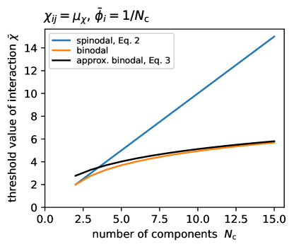
Figure A1: Phase count differs from number of unstable modes in liquids with with identical interactions and symmetric composition. A homogeneous mixture is unstable for interactions ${\bar{\chi}}$ above the spinodal (blue line). In contrast, phase separation is energetically favorable for ${\bar{\chi}}$ above the binodal (orange line). The black line shows the analytical approximation given by Eq. (A5).

For the coexisting phases in equilibrium, we focus on the simples state that the mixture might separate into. Due to permutational symmetry, we assume that each one of the candidate coexisting phases enriches one component with volume fraction $\phi_{\mathrm{h}}=1-({N_{\mathrm{c}}}-1)\phi_{\mathrm{l}}$, while all other components have the same volume fraction $\phi_{\mathrm{l}}$. We will show below that this assumption is reasonable for sufficient large ${\bar{\chi}}$. In this case, the free energy density reads

$$f(\phi_{\mathrm{l}}) =({N_{\mathrm{c}}}-1){\bar{\chi}}\phi_{\mathrm{h}}\phi_{\mathrm{l}}+\frac{({N_{\mathrm{c}}}-1)({N_{\mathrm{c}}}-2)}{2}{\bar{\chi}}\phi_{\mathrm{l}}^{2}+\phi_{\mathrm{h}}\ln\phi_{\mathrm{h}}+({N_{\mathrm{c}}}-1)\phi_{\mathrm{l}}\ln\phi_{\mathrm{l}}\;.$$ (A4)

Note that Eq. (A4) reduces to Eq. (A2) when $\phi_{\mathrm{h}}=\phi_{\mathrm{l}}=1/{N_{\mathrm{c}}}$. Since all coexisting phases have the same free energy density due to permutational symmetry, the coexisting phases are energetically favored over the homogeneous state if the minimal value of Eq. (A4) is lower than that of the homogeneous state given by Eq. (A2). Fig. A1 shows the results from a numerical minimization of Eq. (A4) compared to Eq. (A2).

To obtain an analytical approximation of the minimal interaction strength necessary for phase separation, we note that with $\phi_{\mathrm{l}}\rightarrow+0$, the free energy $f(\phi_{\mathrm{l}})\rightarrow 0$, while its derivative ${\mathrm{d}}f/{\mathrm{d}}\phi_{\mathrm{l}}\rightarrow-\infty$. Using the mean value theorem, we then conclude that Eq. (A4) will have a minimum lower than Eq. (A2) when $f$ given by Eq. (A2) is positive, implying

$${\bar{\chi}}>\frac{2{N_{\mathrm{c}}}}{{N_{\mathrm{c}}}-1}\ln{N_{\mathrm{c}}}\;,$$ (A5)

which is Eq. (4) in the main text.

We further consider the volume fraction of the dilute components in these coexisting phases, which minimizes Eq. (A2). The dilute fraction $\phi_{*}^{({N_{\mathrm{c}}})}$ that minimizes $f$ satisfies the equation

$${\bar{\chi}}=\frac{1}{1-{N_{\mathrm{c}}}\phi_{*}^{({N_{\mathrm{c}}})}}\biggl{(}\ln\left[1-({N_{\mathrm{c}}}-1)\phi_{*}^{({N_{\mathrm{c}}})}\right]-\ln\phi_{*}^{({N_{\mathrm{c}}})}\biggr{)}\;.$$ (A6)

Assuming that $\phi_{*}^{({N_{\mathrm{c}}})}$ is much smaller that $1/{N_{\mathrm{c}}}$, we obtain

$$\phi_{*}^{({N_{\mathrm{c}}})}\approx-\frac{W\left[{N_{\mathrm{c}}}({\bar{\chi}}-1)-1\right]}{{N_{\mathrm{c}}}({\bar{\chi}}-1)-1}\;,$$ (A7)

where $W(r)$ is the Lambert $W$ function, which satisfies $W(r)e^{W(r)}=r$. When ${\bar{\chi}}\gg\ln{N_{\mathrm{c}}}$, the equation above can be further simplified to

$$\phi_{*}^{({N_{\mathrm{c}}})}\overset{{\bar{\chi}}\rightarrow\infty}{\longrightarrow}e^{-{\bar{\chi}}}\;,$$ (A8)

which is independent of ${N_{\mathrm{c}}}$. Note that Eq. (A8) also shows that the assumption $\phi_{*}^{({N_{\mathrm{c}}})}\ll 1/{N_{\mathrm{c}}}$ is valid when ${\bar{\chi}}\gg\ln{N_{\mathrm{c}}}$.

We next show that for sufficient high value of ${\bar{\chi}}$ it is optimal for the system with identical interactions and symmetric composition to separate into phases which each enrich one component. In the case of identical interactions and average volume fractions, the coexisting states in equilibrium must have the same free energy density, which can be proved by contradiction: Assuming coexisting states have different free energy energies in equilibrium, there must exist one of the coexisting states that have the lowest free energy density. Suppose such phase has a volume fraction vector $\boldsymbol{\phi}=[\phi_{1},\phi_{2}\ldots\phi_{N_{\mathrm{c}}}]$, then a new collection of phases can be constructed by permuting the vector. Since all the interactions are identical, these phases share the same free energy density, while the average volume fractions must be symmetric, meaning that the collection itself becomes a valid candidate of the coexisting state. Since this collection has lower free energy density than the original coexisting states, the initial assumption of equilibrium is violated. Taken together, for identical interactions and average volume fractions, all coexisting states must have the same free energy density in equilibrium.

As the result of equal free energy density, the composition of the coexisting phases must be the local minimizer of the free energy function, otherwise a new set of coexisting phases with lower free energy can be found. Therefore, the compositions must satisfy ${\partial f}/{\partial\phi_{i}}=0$, leading to

$$-{\bar{\chi}}\phi_{i}+\ln\phi_{i}=\mathrm{constant}$$ (A9)

for $i=1,2\ldots{N_{\mathrm{c}}}$, where the constant is the same across different $i$. Since the function $-{\bar{\chi}}\phi+\ln\phi$ can at most have two piecewise monotonic domains in $(0,1)$, the equation above can only have at most two solutions, meaning that each component can either be dilute or concentrated, while all the dilute components share the same composition $\phi_{\mathrm{l}}$ and all the concentrated components share the same composition $\phi_{\mathrm{h}}$.

Suppose the system would phase separate into phases that enrich $K$ components with volume fraction $\phi_{\mathrm{h}}$, then in each phase ${N_{\mathrm{c}}}-K$ components are dilute and share the volume fraction $\phi_{\mathrm{l}}$, satisfying $K\phi_{\mathrm{h}}+({N_{\mathrm{c}}}-K)\phi_{\mathrm{l}}=1$. Similar to Eq. (A6), we denote by $\phi_{\mathrm{l}}=\phi_{*}^{({N_{\mathrm{c}}})}$ the volume fraction that minimizes the free energy, which satisfies

$${\bar{\chi}}=\frac{\ln\phi_{\mathrm{h}}-\ln\phi_{\mathrm{l}}}{\phi_{\mathrm{h}}-\phi_{\mathrm{l}}}\;.$$ (A10)

In the limit $\phi_{\mathrm{l}}\ll 1$, we find

$$\phi_{*}^{({N_{\mathrm{c}}})}\approx\frac{1}{K}e^{-K{\bar{\chi}}}\;.$$ (A11)

Since the right hand side decrease monotonically with $K$ for ${\bar{\chi}}>0$, the dilute components become more dilute for large $K$. For sufficient large value of ${\bar{\chi}}$, the enriched components will take over the vast majority of the phase ($\phi_{\mathrm{h}}\approx K^{-1}$), making these enriched components themselves a subsystem with $K$ components with equal interactions and almost the same total volume fraction as the original one. This subsystem will undergo phase separation since the homogeneous state is more prone to phase separation for fewer components; see Fig. A1. Taken together, the system prefers to enrich one component in each phase since the concentrated components would otherwise phase separate from each other. Intuitively, in the identical interactions and symmetric compositions case, all components dislike each other and they just prefer to separate from the others when possible. States that enrich two components are not preferred since there are no other factors, e.g. higher-ordered interactions, to stabilize them [32].

Appendix C Relation between number of unstable modes and composition with identical interactions

We here consider the number of unstable modes averaged over the entire phase diagram for identical interactions, $\chi_{ij}={\bar{\chi}}(1-\delta_{ij})$. The Hessian given by Eq. (A1) can be simplified and rewritten in matrix form,

$$\boldsymbol{H}=\mathrm{diag}\left\{\frac{1}{\phi_{i}}-\chi\right\}_{i=2}^{N_{\mathrm{c}}}+\left(\frac{1}{\phi_{1}}-\chi\right)\boldsymbol{u}\boldsymbol{u}^{T}\;,$$ (A12)

where $\boldsymbol{u}$ is a all-one vector in ${N_{\mathrm{c}}}-1$ dimensions. Denote the rank-$n$ leading minor of $\boldsymbol{H}$ by $\boldsymbol{H}_{n}$,

$$\boldsymbol{H}_{n}=\mathrm{diag}\left\{\frac{1}{\phi_{i}}-\chi\right\}_{i=2}^{n+1}+\left(\frac{1}{\phi_{1}}-\chi\right)\boldsymbol{u}_{n}\boldsymbol{u}_{n}^{T}\;,$$ (A13)

with $n=1,2\ldots{N_{\mathrm{c}}}-1$ and $\boldsymbol{u}_{n}$ is a all-one vector in $n$ dimensions. Making use of Cauchy interlacing theorem, the number of negative eigenvalues of $\boldsymbol{H}$ can be obtained by calculating the number of sign changes in the sequence

$$\det{\boldsymbol{H}_{0}},\det{\boldsymbol{H}_{1}},\ldots,\det{\boldsymbol{H}_{{N_{\mathrm{c}}}-1}}\;,$$ (A14)

where $\det{\boldsymbol{H}_{0}}$ is defined to be 1. Using the Weinstein-Aronszajn identity, $\det{\boldsymbol{H}_{n}}$ can be calculated,

$$\det{\boldsymbol{H}_{n}} =\left(\frac{1}{\phi_{1}}-\chi\right)^{n}\det\mathrm{diag}\left\{\frac{\phi_{i}^{-1}-\chi}{\phi_{1}^{-1}-\chi}\right\}_{i=2}^{n+1}\det\left(\boldsymbol{I}+\boldsymbol{u}_{n}\boldsymbol{u}_{n}^{T}\mathrm{diag}\left\{\frac{\phi_{1}^{-1}-\chi}{\phi_{i}^{-1}-\chi}\right\}_{i=2}^{n+1}\right)$$

$$=\prod_{i=1}^{N_{\mathrm{c}}}\left(\frac{1}{\phi_{i}}-\chi\right)\left(\sum_{i=1}^{N_{\mathrm{c}}}\frac{1}{\frac{1}{\phi_{i}}-\chi}\right).$$ (A15)

We here assume $\phi_{i}^{-1}\neq\chi$ since we are interested in the average behavior over the entire phase diagram, where the points violating this condition have zero measure. Since the number of negative eigenvalues is invariant under any proper rotation, we can also require that sequence

$$\frac{1}{\phi_{1}}-\chi,\frac{1}{\phi_{2}}-\chi,\ldots,\frac{1}{\phi_{N_{\mathrm{c}}}}-\chi$$ (A16)

decreases monotonically. Comparing Eq. (A14) and Eq. (A15) with Seq. A16, we obtain that the number of sign changes in Seq. A14 can only be either the number of negative elements in Seq. A16, denoted by $N_{-}$, or one less, $N_{-}-1$, since the term $\sum_{i=1}^{N_{\mathrm{c}}}1/(\phi_{i}^{-1}-\chi)$ can at most change the sign once itself and cancel the sign changes of $\prod_{i=1}^{N_{\mathrm{c}}}(\phi_{i}^{-1}-\chi)$ once. We thus obtain the relationship between ${N_{\mathrm{u}}}$ and $N_{-}$ given in the main text.

Appendix D Numerical algorithm for finding coexisting phases

There are multiple challenges for determining equilibrium coexisting states in multi-component mixture: First, the optimization problem is high-dimensional. Second, different types of constrains, such as incompressibility and volume conservation, need to be satisfied. In addition, it is generally difficult to conclude whether the obtained coexisting states are the true equilibrium or metastable states.

In a previous publication [11], we already designed an efficient algorithm to obtain coexisting states by exchanging components between compartments, guided by thermodynamic properties such as osmotic pressure and chemical potential. To achieve high performance, the constraint of volume conservation was relaxed, making it difficult to uniformly sample the entire phase diagram, which was highlighted in ref. [10]. To circumvent these challenges, we here design an improved method based on a free energy optimization strategy inspired by polymeric field theories, where the volume conservation is automatically guaranteed by introducing conjugate fields.

The equilibrium coexisting states can be obtained by optimizing the average free energy density given by Eq. (2) in the main text over all possible phase counts and phase compositions. To allow different phase counts, we consider an ensemble of $M$ abstract compartments as proposed in ref. [11], where $M$ is much larger than the number of components ${N_{\mathrm{c}}}$. To alleviate the problem of negative volume fractions during the relaxation dynamics and conserve the average volume fractions, we extend the free energy of Eq. (2) into the form

$$\bar{f} =\sum_{m=1}^{M}J_{m}\left[\frac{1}{2}\sum_{i,j}^{N_{\mathrm{c}}}\chi_{ij}\phi_{i}^{(m)}\phi_{j}^{(m)}-\sum_{i}^{N_{\mathrm{c}}}w_{i}^{(m)}\phi_{i}^{(m)}+\xi_{m}\biggl{(}\sum_{i}^{N_{\mathrm{c}}}\phi_{i}^{(m)}-1\biggr{)}\right]-\sum_{i}^{N}\bar{\phi_{i}}\ln Q_{i}+\eta\biggl{(}\sum_{m}^{M}J_{m}-1\biggr{)},$$ (A17)

with

$$Q_{i}=\sum_{m}^{M}J_{m}\exp\left(-w_{i}^{(m)}\right).$$ (A18)

Here, $J_{m}$ are the relative volumes of the compartments, $w_{i}^{(m)}$ are the conjugate variables of $\phi_{i}^{(m)}$, and $\xi_{m}$ and $\eta$ are the Lagrangian multipliers for incompressibility of each compartment and compartment volume conservation, respectively. Consequently, the extremum of Eq. (A17) with respect to $\xi(x)$ corresponds to incompressibility,

$$\frac{\partial\bar{f}}{\partial\xi_{m}}\propto\biggl{(}\sum_{i}^{N_{\mathrm{c}}}\phi_{i}^{(m)}-1\biggr{)}J_{m}=0\quad\quad\Rightarrow\quad\quad\sum_{i}^{N_{\mathrm{c}}}\phi_{i}^{(m)}=1\;,$$ (A19)

the extremum with respect to $\eta$ corresponds to conservation of the total volume of all compartments,

$$\frac{\partial\bar{f}}{\partial\eta}\propto\sum_{m}^{M}J_{m}-1=0\quad\quad\Rightarrow\quad\quad\sum_{m}^{M}J_{m}=1\;,$$ (A20)

and the extremum with respect to $w_{i}^{(m)}$ defines the relationship between $\phi_{i}^{(m)}$ and $w_{i}^{(m)}$,

$$\frac{\partial\bar{f}}{\partial w_{i}^{(m)}}\propto-\phi_{i}^{(m)}J_{m}+\frac{\bar{\phi_{i}}}{Q_{i}}\exp\left(-w_{i}^{(m)}\right)J_{m}=0\quad\quad\Rightarrow\quad\quad\phi_{i}^{(m)}=\frac{\bar{\phi_{i}}}{Q_{i}}\exp\left(-w_{i}^{(m)}\right).$$ (A21)

By inserting Eqs. (A19)–(A21) into Eq. (A17), Eq. (2) is recovered except for a constant, which has no influences on thermodynamics. To optimize the free energy density given by Eq. (A17), we obtain the self-consistent equations

$$1 =\sum_{i}^{N_{\mathrm{c}}}\phi_{i}^{(m)}$$ (A22a)

$$1 =\sum_{m}^{M}J_{m}$$ (A22b)

$$\phi_{i}^{(m)} =\frac{\bar{\phi_{i}}}{Q_{i}}\exp\left(-w_{i}^{(m)}\right)$$ (A22c)

$$w_{i}^{(m)} =\sum_{j}^{N_{\mathrm{c}}}\chi_{ij}\phi_{j}^{(m)}+\xi_{m}$$ (A22d)

$$-\eta =\frac{1}{2}\sum_{i,j}^{N_{\mathrm{c}}}\chi_{ij}\phi_{i}^{(m)}\phi_{j}^{(m)}-\sum_{i}^{N_{\mathrm{c}}}w_{i}^{(m)}\phi_{i}^{(m)}+\xi_{m}\biggl{(}\sum_{i}^{N_{\mathrm{c}}}\phi_{i}^{(m)}-1\biggr{)}+\sum_{i}\phi_{i}^{(m)}.$$ (A22e)

Accordingly, we design the following iterative scheme

$$Q_{i}^{(m)} =\sum_{m}^{M}\exp\left(-w_{i}^{(m)}\right)J_{m}$$ (A23a)

$$\phi_{i}^{(m)} =\frac{\bar{\phi_{i}}}{Q_{i}^{(m)}}\exp\left(-w_{i}^{(m)}\right)$$ (A23b)

$$\xi_{m} =\frac{1}{{N_{\mathrm{c}}}}\left(\sum_{i}^{{N_{\mathrm{c}}}}w_{i}^{(m)}-\sum_{i,j}^{{N_{\mathrm{c}}}}\chi_{ij}\phi_{j}^{(m)}\right)$$ (A23c)

$$\eta_{m} =-\frac{1}{2}\sum_{i,j}^{N_{\mathrm{c}}}\chi_{ij}\phi_{i}^{(m)}\phi_{j}^{(m)}+\sum_{i}^{N_{\mathrm{c}}}w_{i}^{(m)}\phi_{i}^{(m)}-\xi_{m}\biggl{(}\sum_{i}^{N_{\mathrm{c}}}\phi_{i}^{(m)}-1\biggr{)}-\sum_{i}\phi_{i}^{(m)}$$ (A23d)

$$\bar{\eta} =\sum_{m}^{M}\eta_{m}J_{m}$$ (A23e)

$$w_{i}^{(m)*} =\sum_{j}^{N_{\mathrm{c}}}\chi_{ij}\phi_{j}^{(m)}+\xi^{(m)}$$ (A23f)

$$J_{m}^{*} =J^{(m)}+\eta^{(m)}-\bar{\eta},$$ (A23g)

where the asterisk denotes the output of the iteration. In order to improve numerical stability, we adopt the simple mixing strategy,

$$w_{i}^{(m),\mathrm{new}} =w_{i}^{(m)}+\alpha\left(w_{i}^{(m)*}-w_{i}^{(m)}\right)$$ (A24a)

$$J^{(m),\mathrm{new}} =J_{m}^{*}+\beta\left(J_{m}^{*}-J_{m}\right).$$ (A24b)

Here $\alpha$ and $\beta$ are two empirical constants, which are usually chosen near $10^{-3}$. We note again that in such iteration scheme the problem of negative volume fractions is relieved. However, there is no guarantee that $J_{m}$ is always positive. Although the algorithm does not suffer from negative $J_{m}$, negative $J_{m}$ implies that the system might be outside of the allowed region on the tie hyperplane. To alleviate this, we always use $\beta$ smaller than $\alpha$, and adopt a killing-and-revive strategy to correct the worst cases: Once $J_{m}$ is found to be negative at certain $m$, e.g. $m_{0}$, the corresponding compartment is considered “dead” and is going to be revived by resetting $J_{m_{0}}$ to its initial value. Concomitantly, $J_{m}$ will be renormalized while the corresponding $w_{i}^{(m_{0})}$ will be redrawn from random distributions. The same scheme is used to initialize the simulation, i.e., all compartments are considered “dead” at the beginning of the simulation.

This algorithm does not guarantee that the true equilibrium state is always found. We handle this problem by launching many more compartments than the number of components, $M\gg{N_{\mathrm{c}}}$. In all our numerical results, the number of compartments are at least $M=16{N_{\mathrm{c}}}$. We justified this choice by increasing number of compartments until both the number and the compositions of unique coexisting states do not change. Under such setting, the equilibrium coexisting states are prominently obtained.

Appendix E Control parameters for average phase count with random interactions

In the main text, we showed that with identical interactions, the control parameters and the asymptotic rules for both average number of unstable modes ${\bar{N}_{\mathrm{u}}}$ and average number of coexisting phases ${\bar{N}_{\mathrm{p}}}$ can be obtained analytically. In contrast, for random interactions with zero mean, random matrix theories only grants us access to the control parameter for ${\bar{N}_{\mathrm{u}}}$, but it does not directly reveal anything about ${\bar{N}_{\mathrm{p}}}$. To infer the control parameter for ${\bar{N}_{\mathrm{p}}}$, we exploit connections between the results from the other three known cases. For simplicity, we assume vanishing mean value of the random interactions in this section, unless specified otherwise.

To predict the scaling of ${\bar{N}_{\mathrm{p}}}$ with ${N_{\mathrm{c}}}$ and ${\sigma_{\chi}}$, we first recall the results for ${\bar{N}_{\mathrm{u}}}$ for random interactions. Ignoring the sole outlier in the spectrum of the Hessian matrix given by Eq. (A1), the average number of negative eigenvalues is approximately the number of eigenvalues of the interaction matrix $\chi_{ij}$ smaller than $-1/\phi_{i}=-{N_{\mathrm{c}}}$, when $\phi_{i}=1/{N_{\mathrm{c}}}$. It has been shown that although in the case of asymmetric composition the eigenvalue spectrum will be expanded, but in the limit of larger interaction variance, the shape of the spectrum is dominated by the random interaction matrix[24]. In addition, since we focus on the average behavior over the entire phase diagram, we expect such spectrum expansion has no preference for positive or negative values. Therefore, to find the control parameters, we check the situation of symmetric composition and suppose the result generalizes to the average behavior over the entire phase diagram. Denoting the eigenvalues of $\chi_{ij}$ by $\lambda_{k}$ with $k=1,2\ldots{N_{\mathrm{c}}}-1$, then ${\bar{N}_{\mathrm{u}}}$ can be roughly estimated by

$${\bar{N}_{\mathrm{u}}}\approx E_{{N_{\mathrm{c}}}}[\lambda_{i}<-1/\phi_{i}]=E_{{N_{\mathrm{c}}}}[\phi_{i}>1/(-\lambda_{k})]\quad\text{for}\quad\chi_{ij}\sim\mathcal{N}(0,{\sigma_{\chi}})\;.$$ (A25)

Since $\lambda_{k}$ is distributed according to a semicircle law with radius $2{\sigma_{\chi}}\sqrt{{N_{\mathrm{c}}}}$, we set $\lambda_{k}=2{\sigma_{\chi}}\sqrt{{N_{\mathrm{c}}}}\gamma$, where $\gamma$ is a random variable according to a semicircle law with unit radius. We thus obtain ${\bar{N}_{\mathrm{u}}}\approx E_{{N_{\mathrm{c}}}}[2{\sigma_{\chi}}\sqrt{{N_{\mathrm{c}}}}\gamma<-1/\phi_{i}]=E_{{N_{\mathrm{c}}}}[-\gamma>\sqrt{{N_{\mathrm{c}}}}/{\sigma_{\chi}}]$, indicating that ${\bar{N}_{\mathrm{u}}}$ is governed by the control parameter ${\sigma_{\chi}}/\sqrt{{N_{\mathrm{c}}}}$ when $\chi_{ij}\sim\mathcal{N}(0,{\sigma_{\chi}})$. However, even though this derivation is only approximative, the literature [24] and our numerical data shown in Fig. 3(a) of the main text suggest that the control parameter is still valid when ${\bar{N}_{\mathrm{u}}}$ is obtained for a uniform average over the entire phase diagram.

Although Eq. (A25) provides no direct information about ${\bar{N}_{\mathrm{p}}}$, it strikingly shares the same form as the relations for ${\bar{N}_{\mathrm{u}}}$ for identical interactions $\chi_{ij}\sim\mathcal{N}({\bar{\chi}},0)$, allowing us to build a connection with ${\bar{N}_{\mathrm{p}}}$ by analogy. From Eq. (7) and Eq. (9) in the main text, we obtain

$${\bar{N}_{\mathrm{u}}} \approx E_{{N_{\mathrm{c}}}}[\phi_{i}>1/{\bar{\chi}}]=E_{{N_{\mathrm{c}}}}[\phi_{i}>1/(-\lambda_{k})]\quad\text{for}\quad\chi_{ij}\sim\mathcal{N}({\bar{\chi}},0)$$ (A26a)

$${\bar{N}_{\mathrm{p}}} \approx E_{{N_{\mathrm{c}}}}[\phi_{i}>1/\exp({\bar{\chi}})]=E_{{N_{\mathrm{c}}}}[\phi_{i}>1/\exp(-\lambda_{k})]\quad\text{for}\quad\chi_{ij}\sim\mathcal{N}({\bar{\chi}},0)\;,$$ (A26b)

since in the case of identical interactions the relevant eigenvalues are all equal to $-{\bar{\chi}}$. The only difference between the unstable modes and the phase count in the equations above is that the negative eigenvalue $-\lambda_{k}$ is modified to $\exp(-\lambda_{k})$. Inspired by this, we speculate that such a modification can also be applied to the case of random interactions $\chi_{ij}\approx\mathcal{N}(0,{\sigma_{\chi}})$. We thus propose

$${\bar{N}_{\mathrm{p}}}\approx E_{{N_{\mathrm{c}}}}[\phi_{i}>1/\exp(-\lambda_{k})]\quad\text{for}\quad\chi_{ij}\sim\mathcal{N}(0,{\sigma_{\chi}})\;.$$ (A27)

Since $\lambda_{k}=2{\sigma_{\chi}}\sqrt{{N_{\mathrm{c}}}}\gamma$, and the average value of $\phi_{i}$ is $1/{N_{\mathrm{c}}}$, we further propose that ${\bar{N}_{\mathrm{p}}}\approx E_{{N_{\mathrm{c}}}}[-\ln{N_{\mathrm{c}}}<-2{\sigma_{\chi}}\sqrt{{N_{\mathrm{c}}}}\gamma]$. leading to the control parameter ${\sigma_{\chi}}\sqrt{{N_{\mathrm{c}}}}/\ln{N_{\mathrm{c}}}$, which we verify numerically in the main text.

Appendix F Deviation of the numerically estimated master functions

To confirm the scalings proposed in Eq. (10) in the main text, and the associated master functions shown in Fig. 4, we calculate the relative standard deviations across the selected number of components. Fig. A2a shows that the deviation between the true values of $({\bar{N}_{\mathrm{u}}}+1)/{N_{\mathrm{c}}}$ and the values predicted by the master function $g_{\mathrm{u}}$ is below $5\%$ in the relevant parameter regime of repulsive interactions (${\bar{\chi}}>0$). Fig. A2b shows that the deviation is even smaller for the phase count ${\bar{N}_{\mathrm{p}}}/{N_{\mathrm{c}}}$, showing that it is incredibly well explained by the master function $g_{\mathrm{p}}$ for positive ${\bar{\chi}}$. In both datasets, the relative deviation is higher in the lower left corner of the plot (${\bar{\chi}}<0$ and small ${\sigma_{\chi}}$). This is expected since most cases exhibit a homogeneous system, so the number of unstable modes is close to $0$, while number of coexisting phases is close to $1$. In these cases, the relative standard deviation degenerates to the standard deviation of the $1/{N_{\mathrm{c}}}$, which is apparently high with respect to $1/{N_{\mathrm{c}}}$ itself.

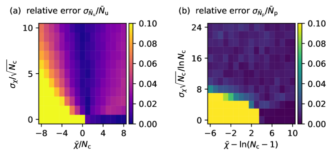
Figure A2: Relative standard deviation of the numerically estimated master functions for ${N_{\mathrm{c}}}\in[16,32]$. (a) Relative standard deviation of number of unstable modes, $\sigma_{{\bar{N}_{\mathrm{u}}}}/{\bar{N}_{\mathrm{u}}}$, and (b) relative standard deviation of number of coexisting phases, $\sigma_{{\bar{N}_{\mathrm{p}}}}/{\bar{N}_{\mathrm{p}}}$, as a function of two scaling variables (a) ${\bar{\chi}}/{N_{\mathrm{c}}}$ and ${\sigma_{\chi}}/\sqrt{{N_{\mathrm{c}}}}$, and (b) ${\bar{\chi}}-\ln({N_{\mathrm{c}}}-1)$ and ${\sigma_{\chi}}\sqrt{{N_{\mathrm{c}}}}/\ln{{N_{\mathrm{c}}}}$, respectively. Standard deviations are calculated for ${N_{\mathrm{c}}}=16,20,24,28,32$.

To validate our result further, we repeat the same procedure for determining the master functions using half the component count ${N_{\mathrm{c}}}$ everywhere. The respective deviations are very similar (compare Fig. A2 and Fig. A4), and comparing Fig. A3 of the main text to Fig. 4 shows that the resulting master functions are very similar. Taken together, this suggests that the master functions shown in Fig. A3 are reliable.

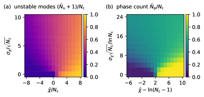
Figure A3: Numerically estimated master functions for ${N_{\mathrm{c}}}\in[8,16]$. Data are averaged over ${N_{\mathrm{c}}}=8,10,12,14,16$. 300-3000 random pairs of interaction matrices and compositions are drawn for each fixed ${N_{\mathrm{c}}}$, ${\bar{\chi}}$ and ${\sigma_{\chi}}$. Other elements are the same as Fig. 4 in the main text.

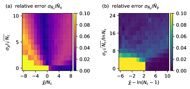
Figure A4: Relative standard deviation of the numerically estimated of master functions for ${N_{\mathrm{c}}}\in[8,16]$. Standard deviations are calculated for ${N_{\mathrm{c}}}=8,10,12,14,16$. 300-3000 samples of random interaction matrices and compositions are drawn for each fixed ${N_{\mathrm{c}}}$, ${\bar{\chi}}$ and ${\sigma_{\chi}}$. Other elements are the same as Fig. A2.

Appendix G Linear regime of average unstable modes/coexisting phases count with respect to mean interaction

The master functions $g_{\mathrm{u}}$ and $g_{\mathrm{p}}$ shown in Fig. A3 in the main text were only estimated numerically. However, their smooth behavior in the region of large ${\sigma_{\chi}}$ and small ${\bar{\chi}}$ suggests that there is a simpler relationship in this region. To obtain such a relationship, we investigate deviations from the line ${\bar{\chi}}=0$ for small $|{\bar{\chi}}|$.

For the unstable modes, $({\bar{N}_{\mathrm{u}}}+1)/{N_{\mathrm{c}}}$, such relationship can be inferred again from random matrix theory. The eigenvalues of the random interaction matrix are distributed according to the semicircle law with radius $r=2{\sigma_{\chi}}\sqrt{{N_{\mathrm{c}}}}$. Adding a mean value ${\bar{\chi}}$ shifts the distribution by $-{\bar{\chi}}$ accordingly. Therefore, the normalized number of unstable modes will increase roughly by $2r{\bar{\chi}}/(\pi r^{2})={\bar{\chi}}/(\pi{\sigma_{\chi}}\sqrt{{N_{\mathrm{c}}}})$ when ${\bar{\chi}}\ll{\sigma_{\chi}}\sqrt{{N_{\mathrm{c}}}}$, so ${\bar{\chi}}$ leads to a linear correction of $({\bar{N}_{\mathrm{u}}}+1)/{N_{\mathrm{c}}}$. Fig. A5 shows that such a shift collapses the data for various ${\bar{\chi}}$. Note that the shift ${\bar{\chi}}/(\pi{\sigma_{\chi}}\sqrt{{N_{\mathrm{c}}}})$ can be interpreted as the ratio between the control parameter for $({\bar{N}_{\mathrm{u}}}+1)/{N_{\mathrm{c}}}$ in the identical interaction case, ${\bar{\chi}}/{N_{\mathrm{c}}}$, and that in the zero-mean random interaction case, ${\sigma_{\chi}}/\sqrt{{N_{\mathrm{c}}}}$.

We speculate that a similar linear relationship with respect to ${\bar{\chi}}$ holds for the phase count ${\bar{N}_{\mathrm{p}}}/{N_{\mathrm{c}}}$. By comparing the control parameters ${\bar{\chi}}-\ln({N_{\mathrm{c}}}-1)$ and ${\sigma_{\chi}}\sqrt{{N_{\mathrm{c}}}}/\ln{{N_{\mathrm{c}}}}$, we conclude that the shift is proportional to ${\bar{\chi}}\ln({N_{\mathrm{c}}})/({\sigma_{\chi}}\sqrt{{N_{\mathrm{c}}}})$. We also include a fitting parameter $\lambda$ since we have little knowledge of the analytical form of $g_{\mathrm{p}}$, in contrast to $g_{\mathrm{u}}$. Fig. A6a shows that shifting the ${\bar{N}_{\mathrm{p}}}/{N_{\mathrm{c}}}$ data according to $\lambda{\bar{\chi}}\ln({N_{\mathrm{c}}})/({\sigma_{\chi}}\sqrt{{N_{\mathrm{c}}}})$ collapses the data for various ${\bar{\chi}}$ over a broad range. The fitting parameter is chosen to be $0.2$, independent of ${N_{\mathrm{c}}}$ (Fig. A6b). Note that these two linear relationships indicate that in the large ${N_{\mathrm{c}}}$ limit, the influences of mean interaction ${\bar{\chi}}$ is subtle, since both $1/(\pi{\sigma_{\chi}}\sqrt{{N_{\mathrm{c}}}})$ and $\ln{{N_{\mathrm{c}}}}/\sqrt{{N_{\mathrm{c}}}}$ are vanishingly small with large ${N_{\mathrm{c}}}$, consistent with Fig. 4.

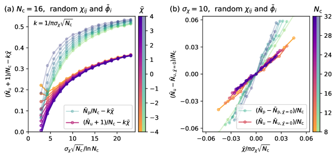
Figure A5: Linear correction proportional to ${\bar{\chi}}$ collapses data of the number of unstable modes. (a) Shifted normalized average number of unstable modes (orange-purple) and coexisting phases (green-blue) as a function of the scaled standard deviation of the interactions for various mean interactions ${\bar{\chi}}$ at fixed component count ${N_{\mathrm{c}}}=16$. The shift coefficient $k=1/\pi{\sigma_{\chi}}\sqrt{{N_{\mathrm{c}}}}$. (b) Changes in the normalized average number of unstable modes (orange-purple) and coexisting phases (green-blue) as a function of the scaled mean interactions for various component counts ${N_{\mathrm{c}}}$ at fixed standard deviation of the interactions, ${\sigma_{\chi}}=10$.

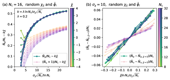
Figure A6: Linear correction proportional to ${\bar{\chi}}$ collapses data of the number of coexisting phases. (a) Shifted normalized average number of unstable modes (orange-purple) and coexisting phases (green-blue) as a function of the scaled standard deviation of the interactions for various mean interactions ${\bar{\chi}}$ at fixed component count ${N_{\mathrm{c}}}=16$. The shift coefficient $k=\lambda\ln{N_{\mathrm{c}}}/{\sigma_{\chi}}\sqrt{{N_{\mathrm{c}}}}$, where $\lambda$ is a fitting constant independent of ${N_{\mathrm{c}}}$. (b) Changes in the normalized average number of unstable modes (orange-purple) and coexisting phases (green-blue) as a function of the scaled mean interactions for various component counts ${N_{\mathrm{c}}}$ at fixed standard deviation of the interactions, ${\sigma_{\chi}}=10$.