DynaMo: Accelerating Language Model Inference with Dynamic Multi-Token Sampling

Abstract

Traditional language models operate autoregressively, i.e., they predict one token at a time. Rapid explosion in model sizes has resulted in high inference times. In this work, we propose DynaMo, a suite of multi-token prediction language models that reduce net inference times. Our models dynamically predict multiple tokens based on their confidence in the predicted joint probability distribution. We propose a lightweight technique to train these models, leveraging the weights of traditional autoregressive counterparts. Moreover, we propose novel ways to enhance the estimated joint probability to improve text generation quality, namely co-occurrence weighted masking and adaptive thresholding. We also propose systematic qualitative and quantitative methods to rigorously test the quality of generated text for non-autoregressive generation. One of the models in our suite, DynaMo-7.3B-T3, achieves same-quality generated text as the baseline (Pythia-6.9B) while achieving 2.57$\times$ speed-up with only 5.87% and 2.67% parameter and training time overheads, respectively.

DynaMo: Accelerating Language Model Inference with Dynamic Multi-Token Sampling

Shikhar Tuli^1,2, Chi-Heng Lin², Yen-Chang Hsu², Niraj K. Jha¹, Yilin Shen², Hongxia Jin^{2 1}Department of Electrical and Computer Engineering, Princeton University ²Samsung Research America {shikhar.tuli,chiheng.lin,yenchang.hsu,yilin.shen,hongxia.jin}@samsung.com, jha@princeton.edu

1 Introduction

Recent research has demonstrated the tremendous promise of large language models (LLMs) as competent artificial intelligence (AI) assistants (Touvron et al., 2023b). This has led to their rapid and widespread adoption as chatbots in diverse applications, e.g., healthcare, e-commerce, education, etc. However, the high computational requirements of LLM training and inference and the use of massive closed-source corpora have restricted their development to a few laboratories. The increasing number of open-source LLMs, including Pythia (Biderman et al., 2023) and LLaMA-2 (Touvron et al., 2023b), democratizes research in natural language processing (NLP). For instance, Vicuna-13B (Chiang et al., 2023), an instruction-finetuned LLaMA model (Touvron et al., 2023a), has gained significant interest among researchers due to its exceptional instruction-following capabilities for its relatively compact size. Nevertheless, access and study of LLMs remain limited due to challenges involved in their efficient evaluation on resource-constrained devices.

Figure 1: Multi-token prediction in DynaMo. (a) Traditional autoregressive prediction requires three forward passes. (b) Non-autoregressive multi-token prediction requires only one forward pass.

1.1 Challenges and Motivation

LLM training and inference are typically limited to large GPU clusters in data centers, causing high latencies and privacy concerns for end-users. Edge computing offers a promising solution by processing data closer to the source, reducing latency and costs while enhancing data security and privacy. However, efficient deployment of conversational AI agents on resource-constrained edge platforms remains challenging, as even compact language models result in significant latencies (Wang et al., 2020a; Tuli and Jha, 2023b). Increasing model sizes exacerbates this issue (Kaplan et al., 2020), highlighting the need for significant inference/text-generation speed-ups and a range of models tailored to diverse platforms with varying resource constraints.

Existing models, trained with the causal language modeling (CLM) objective, predict one token at a time (Radford et al., 2019; Brown et al., 2020). We conceptualize such models as $V$-way ($V$ is the vocabulary size) classifiers or unigram predictors. Mathematically, given the context, i.e., the set of past tokens ${\mathbf{x}}_{1:t}:={\mathbf{x}}_{1},{\mathbf{x}}_{2},\ldots,{\mathbf{x}}_{t}$, traditional LLMs model the probability distribution $p({\mathbf{x}}_{t+1}|{\mathbf{x}}_{1:t})=f_{\theta}({\mathbf{x}}_{1:t})$, where $f_{\theta}$ is the LLM parameterized by $\theta$. In this context, traditional models generate sequences of text autoregressively. In other words, we sample ${\mathbf{x}}_{t+1}$ from $f_{\theta}({\mathbf{x}}_{1:t})$ and then concatenate it with the input sequence to produce ${\mathbf{x}}_{1:t+1}:={\mathbf{x}}_{1},{\mathbf{x}}_{2},\ldots,{\mathbf{x}}_{t},{\mathbf{x}}_{t+1}$. Then, we sample ${\mathbf{x}}_{t+2}$ from the predicted distribution $f_{\theta}(x_{1:t+1})$. Fig. 1(a) shows a schematic of this process with existing autoregressive LLMs.

Research in psycholinguistics shows that humans do not necessarily think of words one at a time when articulating thought (Sridhar, 2012); instead they employ a parallel network of cognitive and linguistic processes. In line with this, we propose predicting multiple tokens simultaneously to accelerate inference. By estimating $p({\mathbf{x}}_{t+1:t+3}|{\mathbf{x}}_{1:t})=f_{\theta}$ (now, a $V^{3}$-way classifier), we aim to achieve reliable multi-token prediction, potentially resulting in a 3$\times$ inference speed-up (assuming no latency overhead). However, simultaneous prediction of three tokens may compromise generation quality (we provide sample generations in Appendix D). Hence, there is a need to dynamically back off to lower-order $n$-gram prediction when the model lacks confidence.

1.2 Our Contributions

In this work, we propose DynaMo: a suite of dynamic multi-token prediction language models. We target inference speed-up by improving upon traditional LLMs in terms of model architecture, training methodology, and non-autoregressive decoding schemes. Further, we propose novel methods to evaluate multi-token prediction for the next generation of non-autoregressive models. More concretely, we summarize the contributions of this work next.

• We augment the suite of Pythia (Biderman et al., 2023) models for multi-token prediction. We explore various architectures for multi-token prediction (label shifts, masking strategies, multi-token heads, etc.). Further, we devise efficient ways to train augmented versions of existing pre-trained LLMs for multi-token prediction.

• We propose novel ways to dynamically predict multiple tokens based on the current context and probabilities of predicted tokens. We model the joint probability distributions of predicted tokens and back off to lower-order $n$-gram prediction when the joint probabilities are not above a given threshold ($\epsilon_{b}$). We propose co-occurrence weighted masking and adaptive thresholding to improve generated text quality.

• We perform rigorous experiments to evaluate the downstream performance of our proposed models. We show that training with our modified-CLM objective enhances the first token prediction quality as well. We evaluate the open-ended text generation quality of our models and its dependence on model size, desired speed-up, and multi-token prediction hyperparameters (e.g., $\epsilon_{b}$). In fact, this is the first non-greedy, non-batched-parallel-decoding work that proves to deliver same-quality generation as the base model with systematic qualitative and quantitative tests.

The rest of the article is organized as follows. Section 3 details the multi-token prediction methodology adopted in the DynaMo suite of models along with the proposed evaluation methods. Section 4 presents the experimental results. Section 5 discusses the implications of multi-token prediction and points out future work directions. Finally, Section 6 concludes the article.

2 Background and Related Works

Previous research explores various approaches to reduce token prediction latency in LLMs. It includes distillation (Hinton et al., 2015), complexity reduction (Wang et al., 2020b), sparsification (Jaszczur et al., 2021), quantization (Shen et al., 2020), etc., to reduce model size or complexity, leveraging specialized hardware (Tuli and Jha, 2023a). Other engineering solutions include Flash attention (Dao et al., 2022) that reduces memory reads/writes. Recently, skeleton-of-thought decoding (Ning et al., 2023) was proposed, wherein the LLM first generates the skeleton of the answer and then conducts batched decoding to complete the contents of each skeleton point in parallel.

Speculative decoding (Stern et al., 2018; Chen et al., 2023a) is yet another approach that has gained recent prominence. It leverages a small draft model (which can be combined with the main model, Cai et al. 2023) to anticipate the main model predictions and queries it for batch verification. The batch size depends on the targeted number of token positions in the future, for draft prediction, and the number of top-$k$ samples at each position. Despite attempts at improving inference efficiency (Spector and Re, 2023; Liu et al., 2023), such methods incur high computational overhead due to high-batch operations and result in poor compute utilization (e.g., sparse tree attention used by Cai et al. 2023; Spector and Re 2023). For the greedy decoding scheme, such methods enable up to $n\times$ speed-up, however, at the cost of at least $n\times$ the compute. Instead, in this work, we propose a low-compute approach that directly maps the joint probability distribution and implements co-occurrence weighted masking and adaptive thresholding, obviating the need for batched verification. Further, Medusa (Cai et al., 2023) exploits simple feed-forward layers for draft prediction. This work explores various architectural modifications for draft prediction. Nevertheless, the abovementioned approaches are orthogonal to the proposed method and can be used in conjunction to further boost performance.

3 Method

In this section, we discuss the implementation details of multi-token prediction in the DynaMo suite.

3.1 Going Beyond One-token Prediction

We propose a modified-CLM objective for multi-token prediction,

$$\mathcal{L}_{\text{T}n}=-\frac{1}{N}\sum_{j=1}^{N}\sum_{t=1}^{L-n+1}\log p({\mathbf{x}}_{t+n}^{j}|{\mathbf{x}}_{1:t}^{j})$$ (1)

for the $n^{th}$-token head. Here, $N$ is the number of sequences in the training set and the length of the $j^{th}$ sequence is $L$. The first-token head predicts the labels shifted by one position. The second-token head predicts the labels shifted by two positions, and so on. Note that the above equation trains each token head to predict the tokens independently. We approximate the joint probability distribution using independent token predictions. We represent this mathematically as follows:

$$\begin{split}p({\mathbf{x}}_{t+1:t+n}|{\mathbf{x}}_{1:t})&=\prod_{i=1}^{n}p({\mathbf{x}}_{t+i}|{\mathbf{x}}_{1:t+i-1})\\ &\approx\prod_{i=1}^{n}p({\mathbf{x}}_{t+i}|{\mathbf{x}}_{1:t})=\prod_{i=1}^{n}f_{\theta}^{i}({\mathbf{x}}_{1:t})\end{split}$$ (2)

where $f_{\theta}^{i}({\mathbf{x}}_{1:t})$ is the prediction by the $i$-th-token head in the DynaMo model.

We use the Pythia (Biderman et al., 2023) suite of models as base models. All decoder layers up to the penultimate layer form the model “stem” (like the stem of a plant). The final decoder layer of the base model and the output embedding form the first-token-predicting head (or simply the first-token head). Fig. 1 shows the data flow for the base model in blue. It assumes a base model with only two decoder layers. The first layer of the base model forms the stem for the DynaMo model, while the second layer is part of the first-token head. The other decoder layers (dataflows shown in green) are part of the second- and third-token heads. The output embeddings for these heads reuse the weights of that of the first head. Hence, the extra parameters for this three-token model are from only two extra decoder layers.

Thanks to the above weight transfer process, most weights (the model stem and the first-token head) in an initialized DynaMo model are already trained. Therefore, we train the DynaMo models on a much smaller dataset (5% randomly sampled version of the Pile dataset, Gao et al. 2020) relative to that used to train the Pythia models. This limits the computational overhead of training our models. We provide further details on the training and evaluation methods for our models in Appendix A.1.

3.2 Dynamic Text Generation

Figure 2: Flowchart of the proposed dynamic multi-token prediction pipeline.

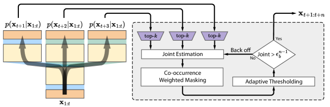
Fig. 2 summarizes the proposed dynamic text generation pipeline. We extend the popular top-$k$ sampling scheme (Fan et al., 2018; Radford et al., 2019) for autoregressive language models to multi-token generation. First, we obtain logits for all token heads. We then obtain the top-$k$ probabilities for the predictions. Then, since we approximate the predicted tokens to be independent, we estimate the joint probability using Eq. (2). We bridge the gap between the true and the estimated (using independent predictions) joint probability distributions using co-occurrence weighted masking, taking inspiration from optimal transport (Peyré et al., 2019). We fix the sparsity in higher-dimensional distributions using adaptive thresholding and backing off to lower-order $n$-gram prediction. We then sample from the joint probability distribution to output the generated sequence of tokens. Hence, DynaMo dynamically generates one or more tokens based on the given context and the model’s confidence in its predictions. We describe the abovementioned methods next.

3.2.1 Co-occurrence Weighted Masking

To bridge the gap between the true and the estimated joint probability distribution in Eq. (2), we mask the estimated distribution using the co-occurrence weights. Mathematically,

$$\begin{split}p({\mathbf{x}}_{t+1:t+n}&|{\mathbf{x}}_{1:t})\\ &=\prod_{i=1}^{n}p({\mathbf{x}}_{t+i}|{\mathbf{x}}_{1:t})\frac{p({\mathbf{x}}_{t+1:t+n}|{\mathbf{x}}_{1:t})}{\prod_{i=1}^{n}p({\mathbf{x}}_{t+i}|{\mathbf{x}}_{1:t})}\\ &\approx\prod_{i=1}^{n}f_{\theta}^{i}({\mathbf{x}}_{1:t})\underbrace{\frac{\hat{p}({\mathbf{x}}_{t+1:t+n})}{\prod_{i=1}^{n}\hat{p}({\mathbf{x}}_{t+i})}}_{\text{co-occurrence mask}}\end{split}$$ (3)

where $\hat{p}({\mathbf{x}}_{t+1:t+n})$ and $\hat{p}({\mathbf{x}}_{t+i})$ are sampled estimates of the joint probability and the prediction of the $i$-th token, respectively. We estimate these probabilities based on the token counts in the training dataset. Note that the approximation in Eq. (3) ignores the history ${\mathbf{x}}_{1:t}$.

Theorem 1.

When the cost function $c({\mathbf{x}}_{t+1},{\mathbf{x}}_{t+2},\ldots,{\mathbf{x}}_{t+n})=-\log\big{(}\frac{\hat{p}({\mathbf{x}}_{t+1:t+n})}{\prod_{i=1}^{n}\hat{p}({\mathbf{x}}_{t+i})}\big{)}$ and $\epsilon_{2}=0$ [defined in Eq. (5)], the joint probability distribution in Eq. (3) is the optimal solution to the optimal transport problem (Peyré et al., 2019).

We describe the optimal transport problem in the multi-token prediction setting and provide a proof of the above theorem in Appendix B.

3.2.2 Dynamic Back-off and Adaptive Thresholding

Intuitively, when generating multiple tokens, the goal is to find the peaks in the predicted joint probability distribution and sample those peaks. If none of the probability values is beyond a threshold (determined by $\epsilon_{b}$), i.e., there are no peaks in the joint probability distribution, our model backs off to lower-order $n$-gram prediction. To implement this, we adopt a static threshold $\epsilon_{b}$. If no probability value is $>\epsilon_{b}^{n-1}$, we back off to sampling a lower-order joint probability distribution. We set all probabilities less than $\epsilon_{b}$ to 0.

Static thresholding is too naïve for joint probability distributions, which can vary with the predicted tokens and input context. Taking inspiration from computer vision methods, we test adaptive thresholding, leveraging Otsu’s binarization algorithm (Otsu, 1979). It adapts the threshold for dynamic back-off based on the predicted joint probability distribution. We apply adaptive thresholding on top of the static thresholding explained above. In other words, we first set all values in the joint probability distribution less than $\epsilon_{b}$ to 0. Then, we set all values less than $\epsilon_{\text{AT}}$ to 0 (where $\epsilon_{\text{AT}}$ is the threshold found using Otsu’s algorithm). In the computer vision domain, researchers implement Otsu’s algorithm after applying Gaussian blur to the input image. We thus explore the effect of using Gaussian blur and adaptive thresholding on the predicted joint probability distribution (ablation analysis in Appendix C.1).

Alg. 1 summarizes the multi-token generation algorithm. We depict the probability distribution output by the $i$-th-token head by $f_{\theta}^{i}$. This probability distribution is a vector of length $V$ (or $k$ after top-$k$ sampling). We calculate the joint probability distribution $\mathbf{J}$ by taking the outer product of the individual token predictions. The function adaptiveThresholding (line 10) implements adaptive thresholding explained above. The function penalizeRepetition (line 12) divides all probabilities that correspond to repetitions by a penalty value (Keskar et al., 2019). The sample function (lines 16 and 20) samples the tokens using multinomial sampling, i.e., weighted by the corresponding probability values. Based on $n$, we output the sequence of generated tokens ${\mathbf{x}}_{t+1:t+n}$. For the proposed set of DynaMo models, we initialize $n=3$. Thus, we dynamically generate new tokens depending on the output predictions (and the corresponding probabilities). A low value of $\epsilon_{b}$ generates more tokens (a three-token model with $\epsilon_{b}=0$ will always generate three tokens). On the other hand, a high value of $\epsilon_{b}$ results in few tokens being generated ($\epsilon_{b}=1$ will always generate only one token).

Algorithm 1 DynaMo multi-token generation

1:input sequence ${\mathbf{x}}_{1:t}$, DynaMo model with token heads $f_{\theta}^{i},\ \forall\ i=1,\ldots,n$.

2:$p({\mathbf{x}}_{t+1}|{\mathbf{x}}_{1:t})\leftarrow f_{\theta}^{1}({\mathbf{x}}_{1:t})$,

3:$p({\mathbf{x}}_{t+2}|{\mathbf{x}}_{1:t})\leftarrow f_{\theta}^{2}({\mathbf{x}}_{1:t})$,

4:$p({\mathbf{x}}_{t+3}|{\mathbf{x}}_{1:t})\leftarrow f_{\theta}^{3}({\mathbf{x}}_{1:t})$,

5:$n=3$ (for three-token model)

6:while $n>1$ do

7:     Obtain top-$k$ values for token predictions $p({\mathbf{x}}_{t+i}|{\mathbf{x}}_{1:t})$

8:     $\mathbf{J}\leftarrow\prod_{i=1}^{n}f_{\theta}^{i}({\mathbf{x}}_{1:t})\frac{\hat{p}({\mathbf{x}}_{t+1:t+n})}{\prod_{i=1}^{n}\hat{p}({\mathbf{x}}_{t+i})}$

9:$\triangleright$ Co-occurrence weighted masking

10:     $\mathbf{J}\leftarrow$ adaptiveThresholding($\mathbf{J}$)

11:$\triangleright$ Adaptive thresholding

12:     $\mathbf{J}\leftarrow$ penalizeRepetition($\mathbf{J}$)

13:     if $j<\epsilon_{b}^{n-1},\ \forall\ j\in\mathbf{J}$ then

14:         $n\leftarrow n-1$ $\triangleright$ Back-off

15:     else

16:         ${\mathbf{x}}_{t+1:t+n}\leftarrow$ sample($\mathbf{J}$)

17:         return ${\mathbf{x}}_{t+1:t+n}$

18:     end if

19:end while

20:return ${\mathbf{x}}_{t+1:t+n}\leftarrow$ sample($p({\mathbf{x}}_{t+1}|{\mathbf{x}}_{1:t})$)

3.3 Evaluation Methods

We propose various methods to evaluate our multi-token models. They include evaluating single-token prediction on standard natural language understanding (NLU) benchmarks, multi-token perplexity, and open-ended generation performance.

3.3.1 NLU Benchmarks

Evaluating multi-token prediction on NLU benchmarks is challenging. This is because most downstream benchmarks only require one-token prediction. However, we hypothesize that training a multi-token prediction transformer results in better prediction of even the first token. We call this a better transformer. We evaluate our models on popular benchmarks with the first-token head. We use the lm-evaluation-harness (Gao et al., 2021) to carry out our evaluations on common benchmarks in both zero-shot and few-shot settings. For fair comparisons, we report the performance of the corresponding base Pythia model as well.

3.3.2 Multi-token Perplexity

To test multi-token text generation quality, we evaluate the models based on perplexity. However, the traditional definition of perplexity is only defined for single token prediction. We extend this to $n^{th}$ token prediction and also $n$-gram prediction. Mathematically,

$$\begin{split}\text{PPL}_{n}&=\exp\left(\mkern-2.0mu-\frac{1}{T}\sum_{t=1}^{T-n}\log p({\mathbf{x}}_{t+n}|{\mathbf{x}}_{1:t})\mkern-2.0mu\right)\mkern-2.0mu,\\ \text{PPL}_{1:n}&=\exp\left(\mkern-2.0mu-\frac{1}{nT}\sum_{t=1}^{T-n}\log p({\mathbf{x}}_{t+1:t+n}|{\mathbf{x}}_{1:t})\mkern-2.0mu\right)\end{split}$$ (4)

For a three-token model, we calculate $\text{PPL}_{1}$, $\text{PPL}_{1:2}$, and $\text{PPL}_{1:3}$. We can also extend perplexity calculation to dynamic multi-token prediction, wherein we decide $n$ based on the joint probability distribution and the back-off threshold. We refer to it as $\text{PPL}_{\text{d}}$. It varies with $\epsilon_{b}$.

Table 1: Zero-shot performance on common sense reasoning tasks.

Model	ARC-c	ARC-e	BoolQ	COPA	HellaSwag	OBQA	PIQA	WinoG
Pythia-70M	15.5±1.0	38.7±1.0	55.9±0.8	53.0±5.0	26.6±0.4	14.6±0.2	58.6±1.2	50.8±1.4
DynaMo-77M-T3	17.3±1.1	41.0±1.0	55.7±0.9	56.0±5.0	26.9±0.4	14.7±1.6	59.8±1.1	49.8±1.4
Pythia-160M	20.7±1.2	44.0±1.0	49.4±0.9	65.0±4.8	29.1±0.5	17.0±1.7	62.0±1.1	50.6±1.4
DynaMo-180M-T3	19.4±1.1	45.3±1.0	48.0±0.9	66.0±4.8	29.3±0.5	16.6±1.7	62.7±1.1	51.7±1.4
Pythia-410M	20.5±1.2	51.6±1.0	58.6±0.9	71.0±4.6	34.5±0.5	17.8±1.7	67.2±1.1	53.3±1.4
DynaMo-430M-T3	21.2±1.2	52.6±1.0	57.1±0.9	70.0±4.6	34.6±0.5	17.9±1.7	67.5±1.1	53.3±1.4
Pythia-1B	24.3±1.2	58.5±1.0	60.8±0.9	74.0±4.4	38.9±0.5	21.8±1.8	70.1±1.1	52.9±1.4
DynaMo-1.1B-T3	25.3±1.3	58.4±1.0	60.9±0.9	76.0±4.3	38.9±0.5	22.2±1.9	70.2±1.1	53.8±1.4
Pythia-1.4B	27.3±1.3	61.8±1.0	58.0±0.9	76.0±4.3	41.7±0.5	22.8±1.9	72.0±1.0	56.9±1.4
DynaMo-1.5B-T3	27.7±1.3	61.5±1.0	59.2±0.9	78.0±4.2	41.9±0.5	22.4±1.9	72.5±1.0	56.0±1.4
Pythia-2.8B	29.9±1.3	53.5±1.0	64.2±0.8	75.0±4.4	45.4±0.5	24.0±1.9	74.1±1.0	58.2±1.4
DynaMo-2.9B-T3	30.4±1.3	64.7±1.0	64.0±0.8	80.0±4.0	45.7±0.5	24.3±1.9	74.2±1.0	59.1±1.4
Pythia-6.9B	33.2±1.4	68.5±1.0	64.4±0.8	74.0±4.4	49.6±0.5	27.0±1.9	75.7±1.0	62.7±1.4
DynaMo-7.3B-T3	33.6±1.4	68.1±1.0	65.1±0.8	76.0±4.3	49.9±0.5	28.0±2.0	75.7±1.0	62.9±1.4

3.4 Open-ended Text Generation

Perplexity is a very restrictive evaluation measure. It constrains model text generation to the text in the validation set. A fairer approach to test multi-token generation would be to evaluate open-ended generated texts. Zheng et al. (2023) propose using strong LLMs like GPT-3.5 (OpenAI, 2023a) and GPT-4 (OpenAI, 2023b) and show that they can match both controlled and crowdsourced human preferences in evaluating generated texts well. Since human evaluation of open-ended generated texts from our models would be very expensive and time-consuming, we use a strong LLM to evaluate the quality of generated text from our DynaMo suite of models.

Vicuna and MT benchmarks (Zheng et al., 2023) require the pre-trained LLM to be finetuned on instruction-following datasets. To disambiguate the effect of instruction finetuning, we evaluate our models with different target speed-ups on a novel sentence-completion benchmark. The task is to complete a sentence for a given prompt. We categorize the sentences into simple declarative, compound declarative, W/H interrogative, Y/N interrogative, affirmative imperative, negative imperative, and exclamatory. We test the text generations of our models for grammatical correctness, creativity, depth, logical flow, coherence, and informativeness of the generated text. The benchmark has ten prompts. For every prompt, we generate ten sentences with different random seeds for every $\epsilon_{b}\in\{0.00,0.02,\ldots,1.00\}$. Thus, for every model, we generate 5100 sentences at different speed-ups. We evaluate the quality of every generated sentence using single-mode and pairwise evaluations. For single-mode evaluation, we ask GPT-3.5 to score the generated response from one to ten. For pairwise evaluation, we ask GPT-3.5 to compare the response against one generated by the corresponding Pythia base model. DynaMo either wins, loses, or ties against the baseline Pythia model. We provide further details on the sentence completion benchmark along with the evaluation setup in Appendix A.3.

Finally, we also evaluate the performance of instruction-finetuned DynaMo models on the Vicuna benchmark. We use the Alpaca dataset (Taori et al., 2023) filtered by GPT-3.5 for high-quality instruction-response pairs (Chen et al., 2023b). The dataset contains 9,229 instruction-response pairs. We follow the evaluation setup from Zheng et al. (2023).

4 Experiments

In this section, we present experimental results and comparisons of the proposed approach with the Pythia baseline, which we used to instantiate the DynaMo models. We provide test results for architectural and training variations in multi-token prediction in Appendix C.2.

4.1 Downstream Performance

We hypothesize that training the decoder layers using the second- and third-token loss terms makes them better. We test this hypothesis next.

We consider eight standard common sense reasoning benchmarks: ARC challenge (ARC-c) and ARC easy (ARC-e, Clark et al. 2018), BoolQ (Clark et al., 2019), COPA (Roemmele et al., 2011), HellaSwag (Zellers et al., 2019), OpenBookQA (OBQA, Mihaylov et al. 2018), PIQA (Bisk et al., 2020), and WinoGrande (WinoG, Sakaguchi et al. 2021). We perform evaluations in the zero-shot setting as done in the language modeling community. Table 1 shows a comparison between each model in the DynaMo suite with that of the corresponding baseline Pythia model. As we can see, DynaMo models outperform their respective baselines on most benchmarks. We report additional downstream performance results in Appendix C.3.

4.2 Multi-token Perplexity

Table 2 shows the multi-token perplexity on the validation set for all models in the DynaMo and Pythia suites. The DynaMo models achieve lower $\text{PPL}_{1}$ relative to their Pythia counterparts due to further training of the first-token head and better decoder layers in the model stem (i.e., all layers up to the penultimate layer). We provide further test results in Appendix C.2. The multi-token perplexity drops as models become larger, making the prediction of multiple tokens easier and better. We describe results for dynamic multi-token perplexity ($\text{PPL}_{\text{d}}$) in Appendix C.4.

Table 2: Multi-token perplexity results for models in the DynaMo and Pythia suites.

Model	$\mathbf{PPL_{1}}$	$\mathbf{PPL_{2}}$	$\mathbf{PPL_{3}}$	$\mathbf{PPL_{1:2}}$	$\mathbf{PPL_{1:3}}$
Pythia-70M	20.2±1.5	-	-	-	-
DynaMo-77M-T3	18.3±1.5	111.4±1.7	262.0±1.6	45.2±1.5	81.2±1.6
Pythia-160M	13.5±1.4	-	-	-	-
DynaMo-180M-T3	12.9±1.4	78.5±1.6	199.4±1.6	31.8±1.5	58.7±1.5
Pythia-410M	9.9±1.4	-	-	-	-
DynaMo-430M-T3	9.6±1.4	59.8±1.6	162.4±1.6	24.0±1.5	45.4±1.5
Pythia-1B	8.5±1.4	-	-	-	-
DynaMo-1.1B-T3	8.4±1.4	44.1±1.6	116.6±1.7	19.3±1.5	35.1±1.6
Pythia-1.4B	7.9±1.6	-	-	-	-
DynaMo-1.5B-T3	7.8±1.6	41.9±2.0	112.7±2.1	18.3±1.9	33.6±1.9
Pythia-2.8B	7.4±1.6	-	-	-	-
DynaMo-2.9B-T3	7.1±1.9	37.1±2.7	100.3±3.0	16.2±2.2	29.8±2.4
Pythia-6.9B	6.6±1.8	-	-	-	-
DynaMo-7.3B-T3	6.5±1.8	31.4±2.6	83.5±3.0	14.4±2.2	25.8±2.4

4.3 Text Generation Performance and Speed-up

We now compare the open-ended text generation performance of the DynaMo models with that of the baseline Pythia models on the sentence-completion benchmark.

Since pairwise evaluations by strong LLMs better align with human evaluations (Zheng et al., 2023), we evaluate our models against the Pythia baseline in the pairwise mode (details in Appendix A.3; single-mode evaluations in Appendix C.5.1). As $\epsilon_{b}$ increases, the text quality improves, but the speed-up decreases. Thus, the win rate (i.e., the number of wins/losses against the baseline) decreases as speed-up increases.

Figure 3: Win rate vs. speed-up for pairwise comparisons on the sentence-completion benchmark with corresponding Pythia models as baselines. GPT-3.5 is used as a judge. Regression plotted with 95% confidence intervals. Same-quality speed-ups are shown in parentheses. Theoretical same-quality speed-ups are marked with an asterisk (*).

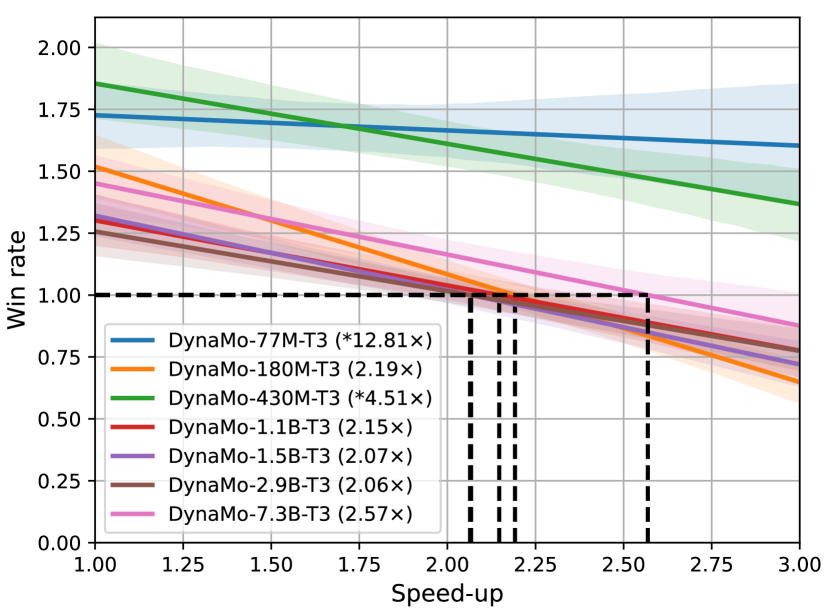
Fig. 3 shows the effect of speed-up on the win rate of the proposed models (we describe how we obtain this plot in Appendix C.5.2). When the win rate is 1.0, the text generation quality would, on average, be the same for the models being compared. We call the speed-up for this case the “same-quality speed-up.” If the win rate for a model is always greater than 1.0, we extrapolate the plot to obtain the “theoretical same-quality speed-up.” However, in further discussions, we refer to the minimum of (theoretical) same-quality speed-up and 3$\times$ (for three-token models) as, simply, the “speed-up.”

4.4 Instruction Finetuning

Figure 4: Pairwise performance of the DynaMo and Pythia models on the Vicuna benchmark. GPT-4 was used as a judge. The actual number of wins, ties, and losses are colored green, yellow, and red, respectively.

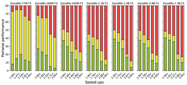
We finetune models in the Pythia and DynaMo suites on an instruction-following dataset (details in Section 3.4). Fig. 4 shows the pairwise performance of the DynaMo (with respect to Pythia) models on the Vicuna benchmark (Zheng et al., 2023). We run the DynaMo models at different speed-ups (we set $\epsilon_{b}=1.0,0.75,0.5,0.25,0.0$) shown on the $x$-axis. We compare each model against the corresponding Pythia baseline. In the case of comparisons with small models, neither model results in a reasonable answer. Hence, GPT-4 classifies many response pairs as ties. The number of ties decreases as model sizes increase. As the speed-up increases, the win rate decreases. DynaMo-7.3B-T3 provides around the same-quality responses as Pythia-6.9B (win rate = 0.98) even for a high speed-up of 2.57$\times$ (we ablate the effect of dynamic text generation methods in Appendix C.1).

5 Discussion

In this section, we discuss the implications of the proposed DynaMo suite of multi-token prediction models and future work directions.

Table 3: Effect of better transformer training on zero-shot performance in common sense tasks.

Model	ARC-c	ARC-e	BoolQ	COPA	HellaSwag	OBQA	PIQA	WinoG
Pythia-70M	15.5±1.0	38.7±1.0	55.9±0.8	53.0±5.0	26.6±0.4	14.6±0.2	58.6±1.2	50.8±1.4
Pythia-70M+	15.6±1.0	38.8±1.0	55.9±0.8	53.1±5.0	26.8±0.4	14.6±0.2	58.6±1.2	50.9±1.4
DynaMo-77M-T3	17.3±1.1	41.0±1.0	55.7±0.9	56.0±5.0	26.9±0.4	14.7±1.6	59.8±1.1	49.8±1.4

5.1 Effect of Better Transformer Training

Another observation that supports the hypothesis that better transformer training results in superior first-token prediction is as follows. For fair comparisons, we test our three-token model against Pythia-70M further trained on the 5% Pile dataset using a learning rate of $10^{-5}$ (we refer to this version as Pythia-70M⁺) on commonsense tasks. We present the result in Table 3 (perplexity results in Appendix C.2.2). Training the decoder layers based on the modified-CLM loss in Eq. (1) results in better first-token prediction, which we use to evaluate common sense tasks as presented here. This key result is worth further exploration, which we leave for future work.

5.2 Contribution of Unigram, Bigram, and Trigram Generations to Speed-up

Figure 5: Percentage of unigram, bigram, and trigram generations vs. $\epsilon_{b}$ for DynaMo-70M-T3.

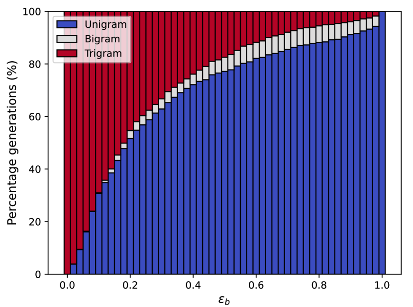
Fig. 5 shows the percentage of one-token, two-token, and three-token generations as we sweep $\epsilon_{b}$ with DynaMo-70M-T3. When $\epsilon_{b}=1.0$, the model always generates one token at a time. When $\epsilon_{b}=0.0$, the model always generates three tokens at a time, regardless of its confidence in the generations. Surprisingly, we note that the contribution of two-token generations is low; the model banks on three-token generations instead. We defer further exploration to balance multi-token generations during dynamic back-off to future work.

5.3 Baseline Comparisons

Table 4 shows comparisons with other approaches that target inference speed-up. Speculative sampling (Chen et al., 2023a) and skeleton-of-thought decoding (Ning et al., 2023) are orthogonal to the DynaMo approach and can be used in conjunction with the proposed multi-token generation scheme to boost performance further. Nevertheless, DynaMo can be seen to require the least overhead in FLOPS-per-generation and provide the highest speed-up. The high computational efficiency of DynaMo is attributed to its avoidance of high-batch operations necessitated by speculative sampling and skeleton-of-thought decoding.

Table 4: Comparisons with other approaches. ^∗Ning et al. (2023) evaluate models of different sizes.

Method	Base Model Size	FLOPS Overhead	Speed-up
Speculative Sampling	70B	340%	1.92-2.46$\times$
Skeleton-of-Thought	7B-13B∗	560%	1.13-2.39$\times$
RecycleGPT	1.3B	15%	1.34-1.40$\times$
DynaMo-77M-T3	70M	8.95%	3.00$\times$
DynaMo-180M-T3	160M	8.73%	2.19$\times$
DynaMo-430M-T3	410M	6.22%	3.00$\times$
DynaMo-1.1B-T3	1B	9.95%	2.15$\times$
DynaMo-1.5B-T3	1.4B	7.12%	2.07$\times$
DynaMo-2.5B-T3	2.4B	5.67%	2.06$\times$
DynaMo-7.3B-T3	6.9B	5.87%	2.57$\times$

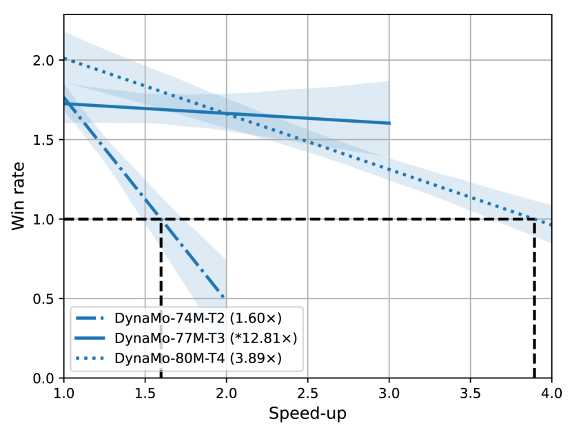
5.4 How Many Tokens Can We Simultaneously Predict?

Fig. 6 shows the win rates with respect to speed-ups on the sentence-completion benchmark using pairwise analysis against Pythia-70M (see Section 3.4 and Appendix A.3). DynaMo-77M-T3 shows much better win rates relative to DynaMo-74M-T2 for speed-ups $<$ 2.0 despite similar $\text{PPL}_{1:2}$. Further, DynaMo-77M-T3, being a three-token model, can provide much higher speed-ups than DynaMo-74M-T2, however, at the cost of a slight parameter overhead. Since the extra parameter overhead is marginal, especially for larger models, we stick with three-token models.

We also explore simultaneous token prediction beyond the three-token model. Fig. 6 also shows the performance of DynaMo-80M-T4. Due to the better transformer training through the modified-CLM objective, the four-token model achieves higher win rates than the three-token counterpart for speed-ups $<$ 2.0. DynaMo-80M-T4 achieves a same-quality speed-up of 3.89$\times$, however, at an additional parameter overhead. Apart from the parameter overhead, the quadruplet co-occurrence mask incurs additional memory overhead. While the pairwise and triplet masks (calculated over 5% of the Pile dataset) only occupy 53.43MB and 152.59MB, respectively, the quadruplet mask (calculated over 0.05% of the Pile dataset) occupies 3.33GB memory. We store all co-occurrence masks using the sparse coordinate format. This overhead may still be negligible for very large models (>7B parameters). We leave simultaneous prediction of more than four tokens and optimized implementation of corresponding co-occurrence masks to future work.

Figure 6: Win rate vs. speed-up for pairwise comparisons on the sentence-completion benchmark with Pythia-70M as the baseline. GPT-3.5 is used as a judge. Theoretical same-quality speed-up is marked with an asterisk (*).

5.5 Additional Benchmarking

We show the performance of the DynaMo models on most downstream benchmarking tasks. These results show that the better transformer trained using loss terms for predicting subsequent tokens generally leads to improved downstream performance while incurring no significant adverse effect on the model’s bias and misinformation abilities (see Appendix C.3.4). While Mukherjee et al. (2023) suggest evaluating world knowledge acquisition through tasks like AGIEval (Zhong et al., 2023) and Big-Bench Hard (Suzgun et al., 2023), we defer assessing larger multi-token models on such complex benchmarks to future work.

6 Conclusion

In this work, we presented DynaMo, a suite of multi-token prediction language models. We trained the proposed model suite efficiently by reusing weights of existing pre-trained LLMs. We proposed novel ways to dynamically predict multiple tokens for a given context. The DynaMo models dynamically back off to lower-order $n$-gram prediction based on a threshold. We also proposed adaptive thresholding and co-occurrence weighted masking on the modeled joint probability distribution to improve text generation quality. One of our proposed models, DynaMo-7.3B-T3, achieved the same-quality generated text as the baseline (Pythia-6.9B) while achieving 2.57$\times$ speed-up with only 5.87% and 2.67% parameter and training time overheads (see Appendix A.2).

7 Limitations

We trained DynaMo models on only 5% of the Pile dataset (Gao et al., 2020). However, training the models on the entire dataset would further boost performance due to improved estimates of the joint probability distributions. Future multi-token models can directly be trained on the entire language corpus without the complex multi-learning-rate learning employed here (details in Appendix A.1). Finally, the current suite of DynaMo models was trained with the Pythia backbone. One could also leverage state-of-the-art open-source foundation models (Touvron et al., 2023b) to train the DynaMo suite.

Appendix A Experimental Setup Details

In this section, we provide details on the training and evaluation processes along with other hyperparameters. We then describe the sentence-completion benchmark. Finally, we present the overheads in training time for our DynaMo suite of models.

A.1 Training and Evaluation Processes

To train the DynaMo suite of models, we first transfer the weights from the base Pythia model. Then, we train the models on a randomly sampled 5% set of sentences in the Pile dataset. We train for one epoch on this dataset. We choose a subset of the same dataset on which the base Pythia model was trained to avoid catastrophic forgetting when being trained on a different dataset. In the future, we plan to train the models on other datasets using standard continual learning approaches (De Lange et al., 2021).

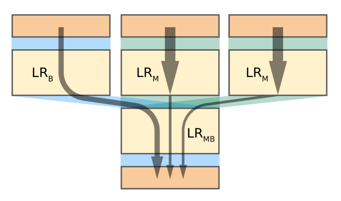
We now describe the training procedure for the DynaMo suite of models. First, we transfer the weights for the base model (i.e., the model stem and the final decoder layer). Then, we train the base model with a low learning rate ($\text{LR}_{\text{B}}$). On the other hand, we train subsequent token heads using a higher learning rate ($\text{LR}_{\text{M}}$) since we randomly initialize their weights. However, when backpropagating those gradients to the model stem, we use a much lower learning rate ($\text{LR}_{\text{MB}}$). We hypothesize that when the decoder layers learn from the first and subsequent token predictions, they make the transformer better in predicting multiple tokens. Table 5 shows the learning rates used for different models in the DynaMo suite. Fig. 7 shows the gradient flow when training an example three-token DynaMo model.

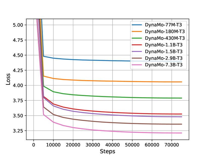
We train our models using the AdamW optimizer (Loshchilov and Hutter, 2017) with the following hyperparameters: $\beta_{1}=0.9,\beta_{2}=0.95,\epsilon=1\times 10^{-8}$. We use the cosine learning rate scheduler such that the learning rate warms up for 1% of the dataset (758 steps) and then drops to 0 at the end of training. We use a batch size of 64 sentences, i.e., 131,072 tokens (each sentence is 2,048 tokens long). The dataset has 5M sentences, which we divide into a training set (97%) and validation set (3%). Thus, a batch size of 64 results in 75,782 training steps in one training epoch. We evaluate the model at every 5,000 steps. Fig. 8 shows the three-token validation loss (logarithm of $\text{PPL}_{1:3}$) for models in the DynaMo suite.

Table 5: Learning rates used for training different models in the DynaMo suite.

Model	$\mathbf{LR_{B}}$	$\mathbf{LR_{M}}$	$\mathbf{LR_{MB}}$
DynaMo-77M-T3	$10^{-5}$	$10^{-3}$	$10^{-6}$
DynaMo-180M-T3	$6\times 10^{-6}$	$6\times 10^{-4}$	$6\times 10^{-7}$
DynaMo-430M-T3	$3\times 10^{-6}$	$3\times 10^{-4}$	$3\times 10^{-7}$
DynaMo-1.1B-T3	$2\times 10^{-6}$	$2\times 10^{-4}$	$2\times 10^{-7}$
DynaMo-1.5B-T3	$2\times 10^{-6}$	$2\times 10^{-4}$	$2\times 10^{-7}$
DynaMo-2.9B-T3	$1.6\times 10^{-6}$	$1.6\times 10^{-4}$	$1.6\times 10^{-7}$
DynaMo-7.3B-T3	$1.2\times 10^{-6}$	$1.2\times 10^{-4}$	$1.2\times 10^{-7}$

Figure 7: Gradient flow when training a DynaMo model.

Figure 8: Loss curves for three-token models in the DynaMo suite.

We train the models on A100 GPUs with 80GB memory. For efficient implementation of our models, we use the flash-attention library (Dao et al., 2022). Our models also support memory-efficient attention in the xformers library (Lefaudeux et al., 2022). Since DynaMo-7.3B-T3 did not fit in memory, we resorted to PyTorch’s fully-sharded data parallel (FSDP) training feature. Table 6 provides the hyperparameters used for the FSDP configuration.

Table 6: FSDP configuration used for training DynaMo-7.3B-T3.

Configuration Key	Value
Sharding strategy	SHARD_GRAD_OP
Transformer-based wrap	DYNAMO_LAYER
All-gather backward prefetch policy	BACKWARD_PRE
All-gather forward prefetch policy	NONE
Mixed precision	FP16

For text generation, we use $k=50$ for top-$k$ decoding, temperature $=0.7$, and repetition penalty $=1.1$. The default text generation hyperparameters for the DynaMo models are $\alpha_{c}=1.0$ (see Appendix C.1), adaptive thresholding with Gaussian blur (kernel size $=3$), and using co-occurrence weighted masking unless otherwise specified.

A.2 Training Overheads

Table 7 shows the overhead of training models in the DynaMo suite. We report training times for modified-CLM training on 5% of the Pile dataset and instruction-finetuning. We present the reported CLM training times for the Pythia models (Biderman et al., 2023).

Table 7: Training (with overheads) and instruction-finetuning times for the DynaMo suite of models.

Model	Training GPU Hrs.	Instruction-FT GPU Mins.
Pythia-70M	510	-
DynaMo-77M-T3	15 (2.94%)	8
Pythia-160M	1,030	-
DynaMo-180M-T3	36 (3.49%)	15
Pythia-410M	2,540	-
DynaMo-430M-T3	46 (1.81%)	30
Pythia-1B	4,830	-
DynaMo-1.1B-T3	80 (1.65%)	60
Pythia-1.4B	7,120	-
DynaMo-1.5B-T3	88 (1.24%)	72
Pythia-2.8B	14,240	-
DynaMo-2.9B-T3	176 (1.24%)	180
Pythia-6.9B	33,500	-
DynaMo-7.3B-T3	896 (2.67%)	864

A.3 Sentence-completion Benchmark

In this section, we provide details of the sentence-completion benchmark. This benchmark is motivated by the Vicuna benchmark (Zheng et al., 2023). However, it is meant for pre-trained LLMs that are not instruction-finetuned. This dissociates any effects of instruction-finetuning from model performance. The benchmark consists of ten prompts requiring the model to complete the sentence. These prompts correspond to sentences of different types. Table 8 outlines the prompts.

Table 8: Prompts in the sentence-completion benchmark.

Prompt	Type
I am a student at the	Simple Declarative
This is going to be a very	Simple Declarative
He wanted to play, but	Compound Declarative
How can we	W/H Interrogative
What will	W/H Interrogative
Will you	Y/N Interrogative
Please explain	Affirmative Imperative
Do not	Negative Imperative
Wow! I can’t believe that	Exclamatory
This is amazing! We	Exclamatory

To obtain the GPT score, we ask GPT-3.5 to rate the generated sentence on a scale from 1 to 10. For pairwise evaluations, we ask GPT-3.5 to compare the generated text (by our DynaMo model) against a baseline (the corresponding baseline Pythia model) and rate it as a “win,” “lose,” or a “tie.” We use gpt-3.5-turbo-0613 for our evaluations. Fig. 9 shows the prompt template used for single-mode evaluations and Fig. 10 shows the prompt template used for pairwise evaluations. However, this benchmark also suffers from the same drawbacks as the Vicuna benchmark (Zheng et al., 2023), which we attempt to alleviate. To address position bias in pairwise comparisons, we randomly order the responses of the assistants.

Figure 9: Prompt template to rate the sentence quality of the candidate assistant model on an absolute scale (single-mode evaluation).

Figure 10: Prompt template to rate the sentence quality of the candidate assistant model against a baseline model (pairwise-mode evaluation).

Appendix B Optimal Transport Theory

Eq. (2) approximates the output joint probability by directly multiplying the independent marginal distributions. This implicitly assumes that ${\mathbf{x}}_{t+2}$ is independent of ${\mathbf{x}}_{t+1}$ conditioned on history ${\mathbf{x}}_{1:t}$, ${\mathbf{x}}_{t+3}$ is independent of ${\mathbf{x}}_{t+1}$ and ${\mathbf{x}}_{t+2}$, and so on. The downside of this decoding strategy is that it ignores the fact that the prediction of ${\mathbf{x}}_{t+2}$ depends heavily on which ${\mathbf{x}}_{t+1}$ is chosen (and similarly for subsequent predictions). A simple example is to consider ${\mathbf{x}}_{1:t}=$ I; here, to is a plausible second-word prediction as many sentences lead to that word, such as I like to, I want to, and I went to. On the other hand, am is a plausible first-word prediction. However, as long as one chooses it, the weight for to as the second-word prediction should be minimal unless we want to make our English teacher cry. This motivates us to weight the joint probability distribution based on co-occurrence of words (or, more precisely, tokens).

What follows is a theoretical motivation behind the use of co-occurrence weighted masking. Formally, according to optimal transport theory (Peyré et al., 2019), we define a cost function $c({\mathbf{x}}_{t+1},\ldots,{\mathbf{x}}_{t+n}),\ \forall\ {\mathbf{x}}_{t+1},\ldots,{\mathbf{x}}_{t+n}$. Once we define the cost function, we pose the joint estimation problem as follows,

$$\begin{split}\arg\min_{p}&\sum p({\mathbf{x}}_{t+1:t+n}|{\mathbf{x}}_{1:t})c({\mathbf{x}}_{t+1},\ldots,{\mathbf{x}}_{t+n})\\ &\Delta{\mathbf{x}}_{t+1}\ldots\Delta{\mathbf{x}}_{t+n}\\ +\leavevmode\nobreak\ &\epsilon_{1}\text{KL}\left(p({\mathbf{x}}_{t+1:t+n}|{\mathbf{x}}_{1:t})||\prod_{i=1}^{n}f_{\theta}^{i}({\mathbf{x}}_{1:t})\right)\\ +\leavevmode\nobreak\ &\epsilon_{2}\sum_{i=1}^{n}\text{KL}\left(p({\mathbf{x}}_{t+i}|{\mathbf{x}}_{1:t})||f_{\theta}^{i}({\mathbf{x}}_{1:t})\right)\end{split}$$ (5)

Although solving an optimal transport problem is fast, using the celebrated Sinkhorn algorithm (Séjourné et al., 2019), we propose the use of Eq. (3) as an approximation that works well in practice, as we demonstrate in our experimental results. Next, we show that the approximation in Eq. (3) is indeed the closest to preserving the true joint probability distribution, when the correction term (co-occurrence mask) is not dependent on the history ${\mathbf{x}}_{1:t}$.

Figure 11: Joint probability distribution with top 10 tokens sorted in decreasing order of probabilities using the DynaMo-2.9B-T2 model for the input prompt: Please explain. Probabilities corresponding to repetition have been penalized by a factor of 100. (a) and (d) are vanilla distributions. Co-occurrence masked distribution with (b) $\alpha_{c}=0.5$ [CO-0.5] and (c) $\alpha_{c}=1.0$ [CO]. Adaptive thresholding (e) without Gaussian blur [AT], and (f) with Gaussian blur (kernel size = 3) [AT + G-3].

Proof of Theorem 1..

Recall that the optimization in Eq. (5) is subject to the constraint $\int p({\mathbf{x}}_{t+1:t+n}|{\mathbf{x}}_{1:t})\Delta{\mathbf{x}}_{t+1}\ldots\Delta{\mathbf{x}}_{t+n}=1$. Thus, the Lagrangian of the objective is given by

$$L= \sum p({\mathbf{x}}_{t+1:t+n}|{\mathbf{x}}_{1:t})c({\mathbf{x}}_{t+1},\ldots,{\mathbf{x}}_{t+n})$$

$$\Delta{\mathbf{x}}_{t+1}\ldots\Delta{\mathbf{x}}_{t+n}$$

$$+\epsilon_{1}\text{KL}\left(p({\mathbf{x}}_{t+1:t+n}|{\mathbf{x}}_{1:t})||\prod_{i=1}^{n}f_{\theta}^{i}({\mathbf{x}}_{1:t})\right)$$

$$+\epsilon_{2}\sum_{i=1}^{n}\text{KL}\left(p({\mathbf{x}}_{t+i}|{\mathbf{x}}_{1:t})||f_{\theta}^{i}({\mathbf{x}}_{1:t})\right)$$

$$+\lambda\Big{(}\sum p({\mathbf{x}}_{t+1:t+n}|{\mathbf{x}}_{1:t})\Delta{\mathbf{x}}_{t+1}\ldots\Delta{\mathbf{x}}_{t+n}$$

$$-1\Big{)}$$

Setting the derivative of $L$ w.r.t. $p({\mathbf{x}}_{t+1:t+n}|{\mathbf{x}}_{1:t})$ to zero, we get

$$p^{*}( {\mathbf{x}}_{t+1:t+n}|{\mathbf{x}}_{1:t})$$

$$\propto\prod_{i=1}^{n}f_{\theta}^{i}({\mathbf{x}}_{1:t})\ \exp\left(c({\mathbf{x}}_{t+1},\ldots,{\mathbf{x}}_{t+n})/\epsilon_{1}\right)$$

$$=\prod_{i=1}^{n}f_{\theta}^{i}({\mathbf{x}}_{1:t})\frac{\hat{p}({\mathbf{x}}_{t+1:t+n})}{\prod_{i=1}^{n}\hat{p}({\mathbf{x}}_{t+i})}$$

∎

Appendix C Additional Results

In this section, we report additional supporting results.

C.1 Ablation of Dynamic Text Generation Methods

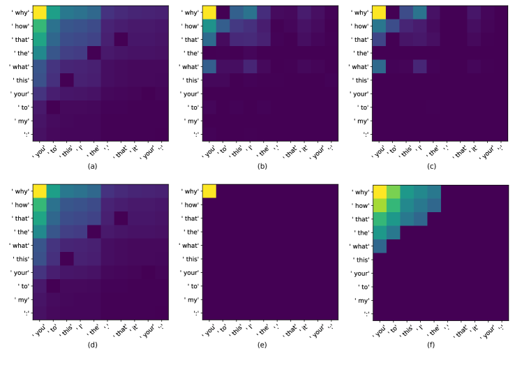
In this section, we ablate the effect of adaptive thresholding (with and without Gaussian blur) and co-occurrence weighted masking (see Section 3.2). Figs. 11(a)-(c) show the effect of co-occurrence masking on the two-token joint probability with decreasing masking transparency $\alpha_{c}$. Mathematically, we modify Eq. (3) for the two-token prediction case as follows:

$$\begin{split}p({\mathbf{x}}_{t+1}&,{\mathbf{x}}_{t+2}|{\mathbf{x}}_{1:t})\\ &\approx f_{\theta}^{1}({\mathbf{x}}_{1:t})f_{\theta}^{2}({\mathbf{x}}_{1:t})\left(\frac{\hat{p}({\mathbf{x}}_{t+1},{\mathbf{x}}_{t+2})}{\hat{p}({\mathbf{x}}_{t+1})\ \hat{p}({\mathbf{x}}_{t+2})}\right)^{\alpha_{c}}\end{split}$$ (6)

where $\alpha_{c}=1.0$ implies that the co-occurrence weights mask the joint probability distribution with no transparency. On the other hand, we do not use co-occurrence masking when $\alpha_{c}=0.0$. Nevertheless, $\alpha_{c}=0.5$ partially masks the joint probability distribution using the co-occurrence weights. Figs. 11(d)-(f) show the effect of adaptive thresholding with and without Gaussian blur.

Figure 12: Ablation analysis using adaptive thresholding (with and without Gaussian blur) and co-occurrence masking. Win rates for pairwise tests against Pythia-70M on the sentence-completion benchmark are shown for different speed-ups. GPT-3.5 is used as the judge. Theoretical same-quality speed-ups are marked with an asterisk (*).

Figure 13: Multi-token prediction using a single-token head. The input sequence is shown below the transformer layer. The model predicts the output sequence above. Attention arrows correspond to the modified CLM objective. The attention masks are shown below the input sequences. (a) T1-L2-M0: labels are shifted by two positions (i.e., the model predicts ${\mathbf{x}}^{\prime}_{t+2}$ with ${\mathbf{x}}_{t}$ as input). Under the modified CLM objective, the model learns to predict ${\mathbf{x}}^{\prime}_{t+2}={\mathbf{x}}_{t+2}$. (b) T1-L2-M(-1)R: labels are shifted by two positions but masks are shifted in the opposite direction (i.e., for predicting ${\mathbf{x}}^{\prime}_{t+2}$, the model can sometimes see ${\mathbf{x}}_{t+1}$).

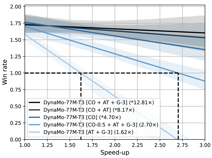
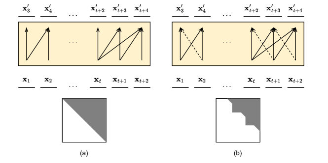
Fig. 12 shows the win rates vs. speed-up for DynaMo-77M-T3, where we generated the texts in the sentence-completion benchmark using difference schemes. We observe that co-occurrence masking (with $\alpha_{c}=1.0$, i.e., the default setting used in our experiments) used along with adaptive thresholding (after application of Gaussian blur with a kernel size $=$ 3) results in the flattest win rate vs. speed-up curve, thus, providing the highest theoretical same-quality speed-up.

We ablate the effect of dynamic text generation methods with the instruction-finetuned DynaMo-7.3B-T3 model on the Vicuna benchmark in Table 9. We take the case $\epsilon_{b}=0.5$ (that results in 2.57$\times$ speed-up in Fig. 4) and present the win rates against Pythia-6.9B. Leveraging co-occurrence weighted masking along with adaptive thresholding using Gaussian blur (kernel size $=$ 3) results in the highest win rate.

Table 9: Ablations analysis of dynamic text generation methods with the instruction-finetuned DynaMo-7.3B-T3 model on the Vicuna benchmark. We use $\epsilon_{b}=0.5$.

Method	Speed-up	Win rate
CO + AT + G-3	2.57$\times$	0.98
CO + AT	2.44$\times$	0.96
CO	2.61$\times$	0.82
CO-0.5 + AT + G3	2.55$\times$	0.77
AT + G-3	2.49$\times$	0.38

C.2 Exploration of Multi-token Prediction Methods

In this section, we provide a detailed overview of various architectural and training variations tested for multi-token prediction.

C.2.1 Design Variations

Under the CLM objective, the attention mask prevents the model from seeing future tokens, i.e., we only compute the attentions corresponding to the lower triangular matrix (we refer to this case as M0). In summary, we represent traditional autoregressive models as T1-L1-M0. We study different variations of the above formulation for multi-token prediction. These include multiple token heads, label shifts, and mask shifts. We explore them below. After testing various approaches, we observe that for, say, three-token prediction, the T3-L1-M0 set of choices performs the best. Thus, in all discussions in the main paper, we represent DynaMo-T3-L1-M0 as simply DynaMo-T3.

Fig. 13 shows the information flow for T1-L2-M0 and T1-L2-M(-1)R cases. In the former case, for predicting ${\mathbf{x}}_{t+2}$, the model only sees the input context ${\mathbf{x}}_{1:t}$. Hence, we shift the mask in the latter case. However, T1-L2-M(-1) would be equivalent to the traditional T1-L1-M0 (ignoring residual connections that result in information leakage). Hence, we randomly mask out some tokens so that the model learns to predict the next and the second-next token at each position. Another position-equivalent modeling approach to T1-L2-M(-1)R is T1-L1-M1R. However, both these modeling approaches suffer from information leakage. T1-L2-M(-1)R suffers from information leakage due to expanding receptive fields along model depth. We fix this by incorporating negative mask shifts only in the first layer of the LLM. T1-L1-M1R suffers from information leakage due to the residual/skip connections in the LLM. Hence, we do not use this approach and test T1-L2-M(-1)R instead.

Figure 14: Architectural variations of the two-token prediction model that we tested: (a) DynaMo-96M-T2, (b) DynaMo-74M-T2 (C), (c) DynaMo-70M-T2 (LoRA), (d) DynaMo-99M-T2, (e) DynaMo-74M-T2 (NP), and (f) DynaMo-77M-T2.

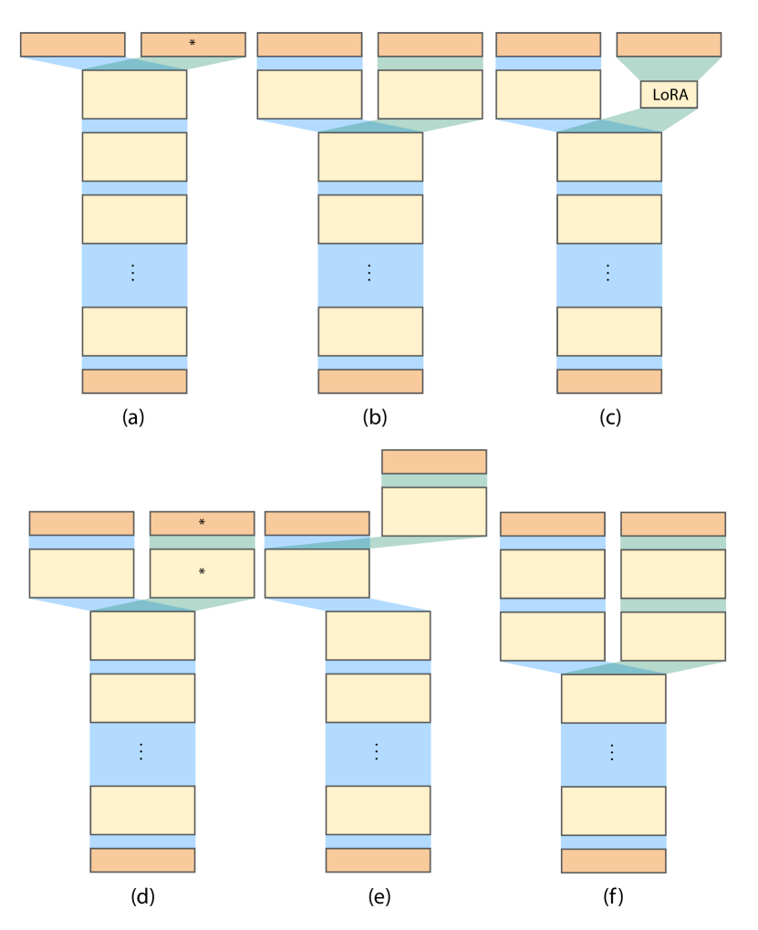
Fig. 14 shows different architectural variations of the two-token model we tested. We initialize all these models from the base Pythia-70M model. Fig. 14(a) shows the schematic of DynaMo-96M-T2 that randomly initializes the output embedding for the second-token head (we denote newly initialized weights by $\ast$ while other variations reuse these weights). The output embedding has 26M trainable parameters. Fig. 14(b) shows DynaMo-74M-T2 (C), which copies the weights of the decoder layer for the second-token head from the last layer of the first-token head (or the base model). Its output embedding for the second-token head reuses the weights from the first-token head. Since we copy the weights, we train the copied weights with a low learning rate ($\text{LR}_{\text{B}}$). Fig. 14(c) shows DynaMo-70M-T2 (LoRA) with only 65K trainable parameters (Hu et al., 2021). The LoRA module includes a low-rank matrix (we use rank $=$ 32). We add its output to that of the last decoder layer for second-token prediction. Fig. 14(d) shows DynaMo-99M-T2. We train a decoder layer and the output embedding for the second-token head, where we randomly initialize the weights of both modules. Fig. 14(e) shows DynaMo-74M-T2 (NP), where we feed the output of the last layer of the base model to the decoder layer for the second-token head. All models in the DynaMo suite use the outputs of the penultimate layer of the base model for subsequent token prediction. Instead, this model uses the output of the final (non-penultimate or NP) layer. Finally, Fig. 14(f) shows the use of two decoder layers for the second-token head.

C.2.2 Evaluations

Table 10: Multi-token perplexity results for various architectural variations. ⁺Model was further trained on 5% Pile dataset.

Model	$\mathbf{PPL_{1}}$	$\mathbf{PPL_{2}}$	$\mathbf{PPL_{3}}$	$\mathbf{PPL_{12}}$	$\mathbf{PPL_{123}}$
Pythia-70M	20.2±1.5	-	-	-	-
Pythia-70M+	20.1±1.5	-	-	-	-
DynaMo-70M-T1-L2	21.4±1.6	1455.8±6.4	-	189.3±2.2	-
DynaMo-70M-T1-L2-M(-1)R	20.3±1.5	645.3±1.9	-	87.4±1.7	-
DynaMo-96M-T2	19.9±1.5	252.4±1.9	-	68.0±1.5	-
DynaMo-74M-T2 (C)	18.3±1.5	296.4±1.5	-	73.7±1.5	-
DynaMo-70M-T2 (LoRA)	20.2±1.5	1368.1±1.8	-	161.2±1.6	-
DynaMo-74M-T2 (CTC)	18.5±1.5	115.4±1.7	-	46.0±1.6	-
DynaMo-99M-T2	18.3±1.5	111.5±1.7	-	45.2±1.5	-
DynaMo-74M-T2 (NP)	18.8±1.5	131.1±1.6	-	49.0±1.5	-
DynaMo-74M-T2-H	20.2±1.5	119.1±1.7	-	49.0±1.5	-
DynaMo-74M-T2	18.3±1.5	112.4±1.7	-	45.4±1.5	-
DynaMo-77M-T2	18.3±1.5	86.7±1.7	-	39.9±1.6	-
DynaMo-77M-T3	18.3±1.5	111.4±1.7	262.0±1.6	45.2±1.5	81.2±1.6

Table 10 shows the multi-token perplexity results for various architectural and training variations of the DynaMo model with Pythia-70M as the baseline. For fair comparisons, we also add the perplexity results for Pythia-70M⁺ (trained using $\text{LR}_{\text{B}}=10^{-5}$). It does not result in a lower $\text{PPL}_{1}$. This shows that with traditional CLM training, $\text{PPL}_{1}$ has converged. However, with the modified-CLM training (details in Appendix A.1), $\text{PPL}_{1}$ for models in the DynaMo suite goes down further. The architectural variations are as explained above. DynaMo-74M-T2 (CTC) shows the perplexity results for the model trained using CTC loss (Yan et al., 2023). DynaMo-74M-T2-H is the model where we only train the decoder layer of the second-token head. Training this model is much faster than training DynaMo-74M-T2, as we need to calculate only a few gradients. However, this does not make the decoder layers in the model stem better. We see that $\text{PPL}_{1}$ of this model is the same as that of Pythia-70M. One could increase the parameter budget for multi-token prediction by either adding another decoder layer for predicting the second token (DynaMo-77M-T2) or using a decoder layer for the third-token head (DynaMo-77M-T3). In the DynaMo suite of models, we traded the parameter budget for higher speed-up (using three-token models). We leave the exploration and search among various architectural decisions (Chitty-Venkata et al., 2022; Tuli and Jha, 2023b) targeting text generation performance and speed-up to future work.

C.3 Additional Downstream Performance Results

We now present additional results on downstream benchmarks.

Table 11: Five-shot exact match performance on the TriviaQA benchmark.

Model	TriviaQA
Pythia-70M	0.2±0.0
DynaMo-77M-T3	0.2±0.0
Pythia-160M	2.1±0.1
DynaMo-180M-T3	2.2±0.1
Pythia-410M	7.4±0.2
DynaMo-430M-T3	7.9±0.2
Pythia-1B	12.0±0.2
DynaMo-1.1B-T3	14.2±0.3
Pythia-1.4B	6.2±0.2
DynaMo-1.5B-T3	18.9±0.3
Pythia-2.8B	7.1±0.2
DynaMo-2.9B-T3	25.1±0.3
Pythia-6.9B	8.9±0.2
DynaMo-7.3B-T3	33.6±0.3

Table 12: Zero-shot accuracy for the RACE benchmark along with exact match performance and F1 scores (in parenthesis) for the SquAD2.0 benchmark.

Model	RACE	SQuAD2.0
Pythia-70M	23.5±1.3	1.2 (2.5)
DynaMo-77M-T3	24.4±1.3	4.2 (5.6)
Pythia-160M	28.3±1.4	0.6 (3.5)
DynaMo-180M-T3	27.9±1.4	0.4 (3.0)
Pythia-410M	31.5±1.4	2.0 (7.4)
DynaMo-430M-T3	32.9±1.5	2.0 (7.2)
Pythia-1B	32.3±1.4	4.2 (5.3)
DynaMo-1.1B-T3	31.9±1.4	4.9 (11.5)
Pythia-1.4B	34.1±1.5	4.4 (5.8)
DynaMo-1.5B-T3	34.0±1.5	6.6 (13.5)
Pythia-2.8B	34.9±1.5	5.2 (8.5)
DynaMo-2.9B-T3	34.5±1.5	7.1 (15.0)
Pythia-6.9B	37.1±1.5	8.0 (9.5)
DynaMo-7.3B-T3	38.3±1.5	11.3 (19.0)

Table 13: Five-shot accuracy on the MMLU benchmark.

Model	Humanities	Social Sciences	STEM	Other	Average
Pythia-70M	24.1±3.0	26.0±3.2	27.6±3.8	23.9±3.2	25.6±3.3
DynaMo-77M-T3	23.6±2.9	27.4±3.3	26.6±3.7	24.8±3.2	25.7±3.3
Pythia-160M	24.2±3.0	26.0±3.2	27.3±3.7	24.1±3.2	25.6±3.3
DynaMo-180M-T3	24.7±3.0	26.6±3.2	25.7±3.6	24.9±3.2	25.5±3.3
Pythia-410M	25.6±3.1	25.0±3.2	26.9±3.7	26.5±3.4	26.1±3.4
DynaMo-430M-T3	25.2±3.1	23.5±3.1	27.7±3.8	27.2±3.4	26.1±3.4
Pythia-1B	25.2±3.0	22.3±3.0	24.0±3.6	25.7±3.3	24.3±3.3
DynaMo-1.1B-T3	24.6±3.0	22.7±3.1	25.2±3.7	26.2±3.3	24.8±3.3
Pythia-1.4B	25.2±3.0	22.4±3.1	27.2±3.8	26.4±3.4	25.5±3.4
DynaMo-1.5B-T3	25.8±3.0	22.2±3.1	27.7±3.8	24.7±3.3	25.4±3.4
Pythia-2.8B	26.5±3.1	25.9±3.2	27.3±3.8	27.8±3.4	27.0±3.4
DynaMo-2.9B-T3	26.6±3.1	24.7±3.2	27.0±3.7	28.2±3.4	26.7±3.4
Pythia-6.9B	26.1±3.1	24.8±3.2	27.3±3.7	26.9±3.4	26.4±3.4
DynaMo-7B-T3	26.3±3.1	25.3±3.1	27.8±3.7	26.6±3.4	26.6±3.4

C.3.1 Closed-book Question Answering

Next, we compare the performance of DynaMo with that of the baseline Pythia models on the TriviaQA closed-book question answering benchmark. We test the five-shot performance of models and report the exact match results. Table 12 shows the results. We can see that the DynaMo models significantly outperform the baselines, especially as the models become larger.

C.3.2 Reading Comprehension

We evaluate the models on the RACE (Lai et al., 2017) and SQuAD2.0 (Rajpurkar et al., 2018) benchmarks in Table 12. Again, DynaMo outperforms Pythia on most model sizes.

C.3.3 Massive Multitask Language Understanding

Next, we report performance on the massive multitask language understanding (MMLU) benchmark, introduced by Hendrycks et al. (2021). It consists of multiple-choice questions that cover various knowledge domains, including humanities, STEM, and social sciences. We present five-shot accuracy results in Table 13. We observe that most models have accuracy close to random chance (25%). Recent literature reports that models trained with much more data break the random performance barrier for these model sizes (Geng and Liu, 2023; Touvron et al., 2023b). We plan to train multi-token counterparts of such models in the future.

C.3.4 Bias and Misinformation

Table 14: Likelihood difference (lower is better) and percentage stereotype (50% is better) on the CrowS-Pairs benchmark along with scores (higher is better) on the MC1 and MC2 tasks in the TruthfulQA benchmark.

Model	CrowS-Pairs		TruthfulQA
	LLD	Stereotype	MC1	MC2
Pythia-70M	3.7±0.1	55.4±1.2	25.3±1.5	47.5±1.6
DynaMo-77M-T3	3.7±0.1	54.9±1.2	25.1±1.5	47.0±1.6
Pythia-160M	4.3±0.1	54.7±1.2	24.7±1.5	44.4±1.5
DynaMo-180M-T3	4.3±0.1	53.6±1.2	24.0±1.5	43.2±1.5
Pythia-410M	3.5±0.1	58.6±1.2	23.6±1.5	41.0±1.5
DynaMo-430M-T3	3.6±0.1	58.7±1.2	23.7±1.5	41.1±1.5
Pythia-1B	3.4±0.1	63.1±1.2	22.6±1.5	38.9±1.4
DynaMo-1.1B-T3	3.5±0.1	63.3±1.2	22.8±1.5	39.3±1.4
Pythia-1.4B	3.5±0.1	61.4±1.2	23.0±1.5	38.6±1.4
DynaMo-1.5B-T3	3.6±0.1	61.0±1.2	23.6±1.5	39.0±1.4
Pythia-2.8B	3.4±0.1	63.4±1.2	21.2±1.4	35.6±1.4
DynaMo-2.9B-T3	3.4±0.1	62.3±1.2	20.4±1.4	35.8±1.4
Pythia-6.9B	3.8±0.1	63.2±1.2	21.7±1.4	35.2±1.3
DynaMo-7.3B-T3	3.7±0.1	62.8±1.2	21.8±1.4	35.2±1.3

Table 14 shows the effect of multi-token training on bias and misinformation in the DynaMo suite of models. We report performance on the CrowS-Pairs (Nangia et al., 2020) and the TrthfulQA benchmarks (Lin et al., 2022). The former tests the model’s biases along nine categories: gender, religion, race/color, sexual orientation, age, nationality, disability, physical appearance, and socioeconomic status. The latter tests the model’s ability to generate false claims, i.e., to hallucinate. We observe that multi-token training does not significantly affect the model’s bias and misinformation abilities.

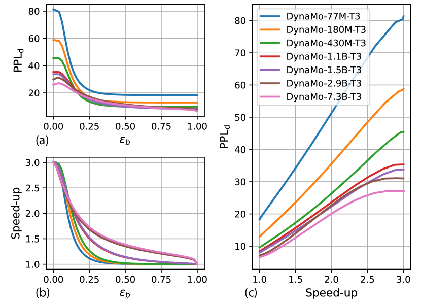
C.4 Dynamic Multi-token Perplexity

For a given threshold $\epsilon_{b}$, the DynaMo model dynamically backs off to lower-order prediction based on input context and predicted joint probability distribution. We calculate the dynamic multi-token perplexity $\text{PPL}_{\text{d}}$ based on the number of tokens generated. Fig. 15 plots $\text{PPL}_{\text{d}}$ against the resultant mean speed-up on the validation set. We observe that $\text{PPL}_{1}$ (i.e., $\text{PPL}_{\text{d}}$ at 1$\times$ speed-up) drops as models become larger. The slope of the curve also reduces. This shows promise for multi-token prediction by larger models beyond those in the current DynaMo suite.

Figure 15: Dynamic multi-token perplexity ($\text{PPL}_{\text{d}}$) for different models in the DynaMo suite. Effect of $\epsilon_{b}$ on (a) $\text{PPL}_{\text{d}}$ and (b) speed-up. (c) Plot of $\text{PPL}_{\text{d}}$ vs. speed-up.

C.5 Sentence Completion Benchmark

We now present additional results on the sentence completion benchmark. We use LLMs trained under the CLM (or modified-CLM) objective to complete the sentence for a given prompt in the sentence-completion benchmark (details in Appendix A.3). We use GPT-3.5 to rate the text generations in single-mode and pairwise evaluations against Pythia.

C.5.1 Single-mode Evaluation

Fig. 16 shows the histograms for the GPT scores on the sentence-completion benchmark for text generations by Pythia-70M and DynaMo-77M-T3. We evaluated 100 generations (ten for each prompt, with a separate random seed) for both models.

Figure 16: Histograms of GPT scores for single-mode evaluations on the sentence-completion benchmark for (a) Pythia-70M and (b) DynaMo-77M-T3 ($\epsilon_{b}=1.0$). GPT-3.5 is used as the judge.

Figure 17: GPT scores for DynaMo-77M-T3 on the sentence-completion benchmark plotted against speed-up. GPT-3.5 is used as the judge. The mean GPT score for Pythia-70M is plotted as a black dashed line. Regression plotted with 95% confidence intervals.

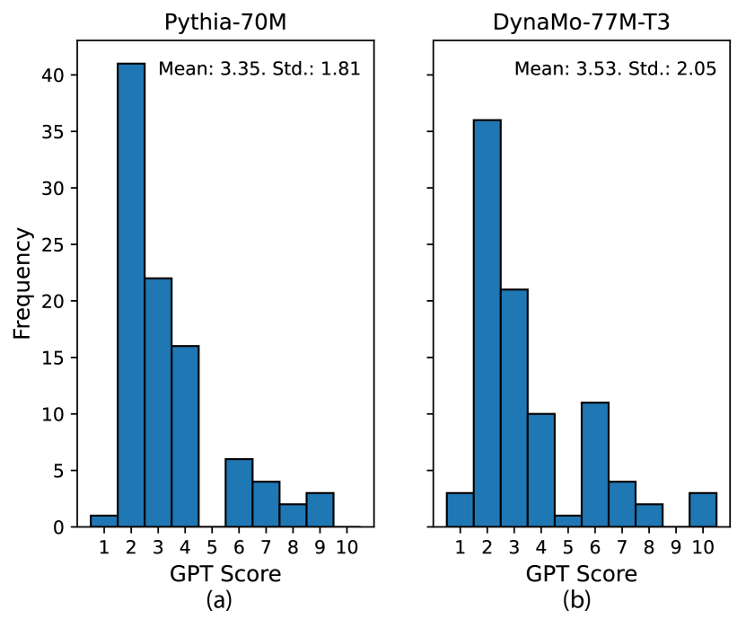
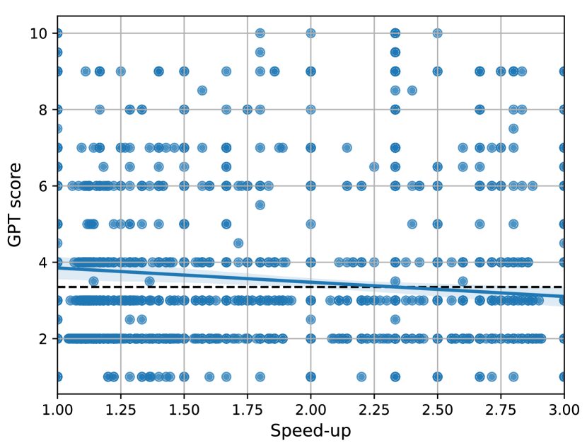
Fig. 17 shows the GPT scores for DynaMo-77M-T3 on the sentence-completion benchmark for different speed-ups. Since the speed-up varies for different text generations (even for the same prompt) with $\epsilon_{b}$, we plot a regression line to predict the GPT for a target speed-up. We leveraged these predicted GPT scores to plot Fig. 18, which shows the evolution of GPT scores with increasing model sizes. We plot the mean GPT scores of the Pythia models. Further, we plot the mean GPT scores of the DynaMo models at different speed-ups. We regress the GPT scores at a target speed-up using GPT score vs. $\epsilon_{b}$ and wallclock speed-up vs. $\epsilon_{b}$ plots. As $\epsilon_{b}$ increases, the GPT score increases, but speed-up decreases. The DynaMo models outperform the baseline at 1$\times$ speed-up, improving performance as the model size increases.

C.5.2 Pairwise Evaluation

Figure 18: Effect of model size on GPT scores. We plot the GPT scores for DynaMo models at different speed-ups. GPT-3.5 used to judge generation quality on a scale 1-10.

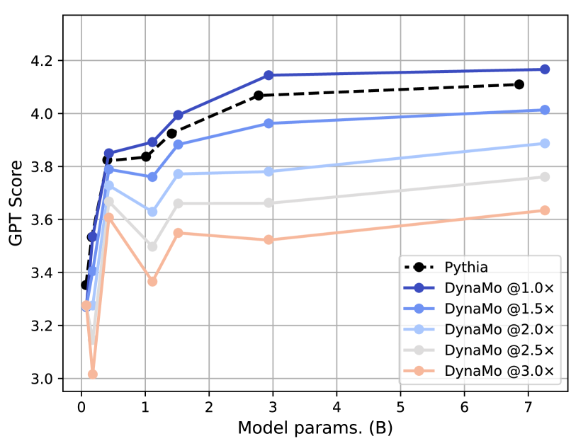
Fig. 19 shows the pairwise performance and speed-ups for DynaMo-77M-T3 against baseline Pythia-70M. For every prompt, at every $\epsilon_{b}$, each bar plots the wins, ties, and losses of DynaMo-77M-T3 over ten text generations (in green, yellow, and red, respectively). We show a regression plot for win-rates (wins/losses) against speed-ups (for different $\epsilon_{b}$’s) in Fig. 3.

Next, we study the effect of model sizes and parameter overheads on the obtained speed-ups. Every DynaMo model instantiated from a base Pythia model trains additional decoder layers for the second- and third-token heads. This results in a parameter overhead for each DynaMo model relative to its Pythia counterpart. Fig. 20 shows that speed-up increases with model size and decreases with parameter overhead, albeit with low statistical significance. Nevertheless, this shows promise for high speed-ups in larger multi-token LLMs. Note that, for the models in the DynaMo suite, model sizes and their parameter overheads are not uncorrelated [see inset in Fig. 20(a)]. Thus, we need more rigorous scaling experiments to test the effect of model sizes and parameter overheads on the obtained speed-up, which we leave to future work.

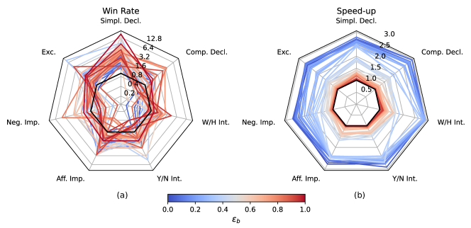
Fig. 21 shows the variation of win rates and speed-ups across different sentence types for the DynaMo-77M-T3 model on the sentence-completion benchmark.

Figure 19: Normalized pairwise performance and speed-ups of DynaMo-77M-T3 on the sentence-completion benchmark plotted against $\epsilon_{b}$.

Figure 20: Speed-up, i.e., the minimum of (theoretical) same-quality speed-up and 3$\times$ for three-token models, with (a) model sizes and (b) parameter overheads. Results are shown for pairwise evaluation on the sentence-completion benchmark. Only points below 3$\times$ speed-up were used to plot the regression line (shown with 95% confidence intervals). Parameter overheads with model sizes are shown in the inset.

Appendix D Sample Text Generations

Figure 21: Pairwise performance on the sentence-completion benchmark categorized by different sentence types. Radar charts for mean (a) win rates and (b) speed-ups for different $\epsilon_{b}$’s are shown.

Figs. 22, 23, and 24 show the generated responses at different speed-ups along with GPT-4’s judgments. We observe that as the target speed-up increases, the grammatical mistakes in the generated response also increase. For 3$\times$ speed-up, DynaMo-7.3B-T3 generated unrelated text. Despite using the repetition penalty, we also observe repetitive $n$-grams generated for smaller models. Grammatical mistakes during multi-token generation should decrease with larger training corpora for subsequent token-head training and with more representative models (e.g., LLaMA-2-70B, Touvron et al. 2023b).

Figure 22: Question, Pythia-6.9B’s and DynaMo-7.3B-T3’s responses at 1$\times$ speed-up, along with GPT-4’s judgements.

Figure 23: Question, Pythia-6.9B’s and DynaMo-7.3B-T3’s responses at 2.62$\times$ speed-up, along with GPT-4’s judgements. A blatant grammatical mistake is highlighted in yellow.

Figure 24: Question, Pythia-6.9B’s and DynaMo-7.3B-T3’s responses at 3$\times$ speed-up, along with GPT-4’s judgements. Blatant grammatical mistakes are highlighted in yellow.

References

- Biderman et al. (2023) Stella Biderman, Hailey Schoelkopf, Quentin Gregory Anthony, Herbie Bradley, Kyle O’Brien, Eric Hallahan, Mohammad Aflah Khan, Shivanshu Purohit, USVSN Sai Prashanth, Edward Raff, et al. 2023. Pythia: A suite for analyzing large language models across training and scaling. In Proceedings of the International Conference on Machine Learning, pages 2397–2430.
- Bisk et al. (2020) Yonatan Bisk, Rowan Zellers, Jianfeng Gao, Yejin Choi, et al. 2020. PIQA: Reasoning about physical commonsense in natural language. In Proceedings of the AAAI Conference on Artificial Intelligence, volume 34, pages 7432–7439.
- Brown et al. (2020) Tom Brown, Benjamin Mann, Nick Ryder, Melanie Subbiah, Jared D Kaplan, Prafulla Dhariwal, Arvind Neelakantan, Pranav Shyam, Girish Sastry, Amanda Askell, et al. 2020. Language models are few-shot learners. Advances in Neural Information Processing Systems, 33:1877–1901.
- Cai et al. (2023) Tianle Cai, Yuhong Li, Zhengyang Geng, Hongwu Peng, and Tri Dao. 2023. Medusa: Simple framework for accelerating LLM generation with multiple decoding heads. https://github.com/FasterDecoding/Medusa.
- Chen et al. (2023a) Charlie Chen, Sebastian Borgeaud, Geoffrey Irving, Jean-Baptiste Lespiau, Laurent Sifre, and John Jumper. 2023a. Accelerating large language model decoding with speculative sampling. arXiv preprint arXiv:2302.01318.
- Chen et al. (2023b) Lichang Chen, Shiyang Li, Jun Yan, Hai Wang, Kalpa Gunaratna, Vikas Yadav, Zheng Tang, Vijay Srinivasan, Tianyi Zhou, Heng Huang, et al. 2023b. AlpaGasus: Training a better Alpaca with fewer data. arXiv preprint arXiv:2307.08701.
- Chiang et al. (2023) Wei-Lin Chiang, Zhuohan Li, Zi Lin, Ying Sheng, Zhanghao Wu, Hao Zhang, Lianmin Zheng, Siyuan Zhuang, Yonghao Zhuang, Joseph E. Gonzalez, Ion Stoica, and Eric P. Xing. 2023. Vicuna: An open-source chatbot impressing GPT-4 with 90%* ChatGPT quality. https://lmsys.org/blog/2023-03-30-vicuna/.
- Chitty-Venkata et al. (2022) Krishna Teja Chitty-Venkata, Murali Emani, Venkatram Vishwanath, and Arun K. Somani. 2022. Neural architecture search for transformers: A survey. IEEE Access, 10:108374–108412.
- Clark et al. (2019) Christopher Clark, Kenton Lee, Ming-Wei Chang, Tom Kwiatkowski, Michael Collins, and Kristina Toutanova. 2019. BoolQ: Exploring the surprising difficulty of natural yes/no questions. In Proceedings of the 2019 Conference of the North American Chapter of the Association for Computational Linguistics: Human Language Technologies, volume 1, pages 2924–2936.
- Clark et al. (2018) Peter Clark, Isaac Cowhey, Oren Etzioni, Tushar Khot, Ashish Sabharwal, Carissa Schoenick, and Oyvind Tafjord. 2018. Think you have solved question answering? Try ARC, the AI2 reasoning challenge. arXiv preprint arXiv:1803.05457.
- Dao et al. (2022) Tri Dao, Dan Fu, Stefano Ermon, Atri Rudra, and Christopher Ré. 2022. FlashAttention: Fast and memory-efficient exact attention with IO-awareness. Advances in Neural Information Processing Systems, 35:16344–16359.
- De Lange et al. (2021) Matthias De Lange, Rahaf Aljundi, Marc Masana, Sarah Parisot, Xu Jia, Aleš Leonardis, Gregory Slabaugh, and Tinne Tuytelaars. 2021. A continual learning survey: Defying forgetting in classification tasks. IEEE Transactions on Pattern Analysis and Machine Intelligence, 44(7):3366–3385.
- Fan et al. (2018) Angela Fan, Mike Lewis, and Yann Dauphin. 2018. Hierarchical neural story generation. In Proceedings of the 56th Annual Meeting of the Association for Computational Linguistics, volume 1, pages 889–898.
- Gao et al. (2020) Leo Gao, Stella Biderman, Sid Black, Laurence Golding, Travis Hoppe, Charles Foster, Jason Phang, Horace He, Anish Thite, Noa Nabeshima, et al. 2020. The Pile: An 800GB dataset of diverse text for language modeling. arXiv preprint arXiv:2101.00027.
- Gao et al. (2021) Leo Gao, Jonathan Tow, Stella Biderman, Sid Black, Anthony DiPofi, Charles Foster, Laurence Golding, Jeffrey Hsu, Kyle McDonell, Niklas Muennighoff, Jason Phang, Laria Reynolds, Eric Tang, Anish Thite, Ben Wang, Kevin Wang, and Andy Zou. 2021. A framework for few-shot language model evaluation. https://doi.org/10.5281/zenodo.5371628.
- Geng and Liu (2023) Xinyang Geng and Hao Liu. 2023. OpenLLaMA: An open reproduction of LLaMA. https://github.com/openlm-research/open_llama.
- Hendrycks et al. (2021) Dan Hendrycks, Collin Burns, Steven Basart, Andy Zou, Mantas Mazeika, Dawn Song, and Jacob Steinhardt. 2021. In Proceedings of the International Conference on Learning Representations.
- Hinton et al. (2015) Geoffrey Hinton, Oriol Vinyals, and Jeff Dean. 2015. Distilling the knowledge in a neural network. arXiv preprint arXiv:1503.02531.
- Hu et al. (2021) Edward J. Hu, Phillip Wallis, Zeyuan Allen-Zhu, Yuanzhi Li, Shean Wang, Lu Wang, Weizhu Chen, et al. 2021. LoRA: Low-rank adaptation of large language models. In Proceedings of the International Conference on Learning Representations.
- Jaszczur et al. (2021) Sebastian Jaszczur, Aakanksha Chowdhery, Afroz Mohiuddin, Lukasz Kaiser, Wojciech Gajewski, Henryk Michalewski, and Jonni Kanerva. 2021. Sparse is enough in scaling transformers. Advances in Neural Information Processing Systems, 34:9895–9907.
- Kaplan et al. (2020) Jared Kaplan, Sam McCandlish, Tom Henighan, Tom B. Brown, Benjamin Chess, Rewon Child, Scott Gray, Alec Radford, Jeffrey Wu, and Dario Amodei. 2020. Scaling laws for neural language models. arXiv preprint arXiv:2001.08361.
- Keskar et al. (2019) Nitish Shirish Keskar, Bryan McCann, Lav R. Varshney, Caiming Xiong, and Richard Socher. 2019. CTRL: A conditional transformer language model for controllable generation. arXiv preprint arXiv:1909.05858.
- Lai et al. (2017) Guokun Lai, Qizhe Xie, Hanxiao Liu, Yiming Yang, and Eduard Hovy. 2017. RACE: Large-scale reading comprehension dataset from examinations. In Proceedings of the Conference on Empirical Methods in Natural Language Processing, pages 785–794.
- Lefaudeux et al. (2022) Benjamin Lefaudeux, Francisco Massa, Diana Liskovich, Wenhan Xiong, Vittorio Caggiano, Sean Naren, Min Xu, Jieru Hu, Marta Tintore, Susan Zhang, Patrick Labatut, and Daniel Haziza. 2022. xFormers: A modular and hackable transformer modelling library. https://github.com/facebookresearch/xformers.
- Lin et al. (2022) Stephanie Lin, Jacob Hilton, and Owain Evans. 2022. TruthfulQA: Measuring how models mimic human falsehoods. In Proceedings of the 60th Annual Meeting of the Association for Computational Linguistics, volume 1, pages 3214–3252.
- Liu et al. (2023) Xiaoxuan Liu, Lanxiang Hu, Peter Bailis, Ion Stoica, Zhijie Deng, Alvin Cheung, and Hao Zhang. 2023. Online speculative decoding. arXiv preprint arXiv:2310.07177.
- Loshchilov and Hutter (2017) Ilya Loshchilov and Frank Hutter. 2017. Decoupled weight decay regularization. arXiv preprint arXiv:1711.05101.
- Mihaylov et al. (2018) Todor Mihaylov, Peter Clark, Tushar Khot, and Ashish Sabharwal. 2018. Can a suit of armor conduct electricity? A new dataset for open book question answering. In Proceedings of the Conference on Empirical Methods in Natural Language Processing, pages 2381–2391.
- Mukherjee et al. (2023) Subhabrata Mukherjee, Arindam Mitra, Ganesh Jawahar, Sahaj Agarwal, Hamid Palangi, and Ahmed Awadallah. 2023. Orca: Progressive learning from complex explanation traces of GPT-4. arXiv preprint arXiv:2306.02707.
- Nangia et al. (2020) Nikita Nangia, Clara Vania, Rasika Bhalerao, and Samuel R. Bowman. 2020. CrowS-pairs: A challenge dataset for measuring social biases in masked language models. In Proceedings of the Conference on Empirical Methods in Natural Language Processing, pages 1953–1967.
- Ning et al. (2023) Xuefei Ning, Zinan Lin, Zixuan Zhou, Huazhong Yang, and Yu Wang. 2023. Skeleton-of-Thought: Large language models can do parallel decoding. arXiv preprint arXiv:2307.15337.
- OpenAI (2023a) OpenAI. 2023a. ChatGPT. https://chat.openai.com.
- OpenAI (2023b) OpenAI. 2023b. GPT-4 Technical Report. arXiv preprint arXiv:2303.08774.
- Otsu (1979) Nobuyuki Otsu. 1979. A threshold selection method from gray-level histograms. IEEE Transactions on Systems, Man, and Cybernetics, 9(1):62–66.
- Peyré et al. (2019) Gabriel Peyré, Marco Cuturi, et al. 2019. Computational optimal transport: With applications to data science. Foundations and Trends in Machine Learning, 11(5-6):355–607.
- Radford et al. (2019) Alec Radford, Jeffrey Wu, Rewon Child, David Luan, Dario Amodei, Ilya Sutskever, et al. 2019. Language models are unsupervised multitask learners. OpenAI Blog, 1(8):9.
- Rajpurkar et al. (2018) Pranav Rajpurkar, Robin Jia, and Percy Liang. 2018. Know what you don’t know: Unanswerable questions for SQuAD. In Proceedings of the 56th Annual Meeting of the Association for Computational Linguistics, volume 2, pages 784–789.
- Roemmele et al. (2011) Melissa Roemmele, Cosmin Adrian Bejan, and Andrew S. Gordon. 2011. Choice of plausible alternatives: An evaluation of commonsense causal reasoning. In Proceedings of the AAAI Spring Symposium Series.
- Sakaguchi et al. (2021) Keisuke Sakaguchi, Ronan Le Bras, Chandra Bhagavatula, and Yejin Choi. 2021. WinoGrande: An adversarial Winograd schema challenge at scale. Communications of the ACM, 64(9):99–106.
- Séjourné et al. (2019) Thibault Séjourné, Jean Feydy, François-Xavier Vialard, Alain Trouvé, and Gabriel Peyré. 2019. Sinkhorn divergences for unbalanced optimal transport. arXiv preprint arXiv:1910.12958.
- Shen et al. (2020) Sheng Shen, Zhen Dong, Jiayu Ye, Linjian Ma, Zhewei Yao, Amir Gholami, Michael W. Mahoney, and Kurt Keutzer. 2020. Q-BERT: Hessian based ultra low precision quantization of BERT. In Proceedings of the AAAI Conference on Artificial Intelligence, volume 34, pages 8815–8821.
- Spector and Re (2023) Benjamin Frederick Spector and Christopher Re. 2023. Accelerating LLM inference with staged speculative decoding. In Workshop on Efficient Systems for Foundation Models@ ICML2023.
- Sridhar (2012) Shikaripur N. Sridhar. 2012. Cognition and Sentence Production: A Cross-linguistic Study, volume 22. Springer Science & Business Media.
- Stern et al. (2018) Mitchell Stern, Noam Shazeer, and Jakob Uszkoreit. 2018. Blockwise parallel decoding for deep autoregressive models. Advances in Neural Information Processing Systems, 31.
- Suzgun et al. (2023) Mirac Suzgun, Nathan Scales, Nathanael Schärli, Sebastian Gehrmann, Yi Tay, Hyung Won Chung, Aakanksha Chowdhery, Quoc Le, Ed Chi, Denny Zhou, and Jason Wei. 2023. Challenging BIG-Bench tasks and whether chain-of-thought can solve them. In Proceedings of the Association for Computational Linguistics, pages 13003–13051.
- Taori et al. (2023) Rohan Taori, Ishaan Gulrajani, Tianyi Zhang, Yann Dubois, Xuechen Li, Carlos Guestrin, Percy Liang, and Tatsunori B. Hashimoto. 2023. Stanford Alpaca: An instruction-following LLaMA model. https://github.com/tatsu-lab/stanford_alpaca.
- Touvron et al. (2023a) Hugo Touvron, Thibaut Lavril, Gautier Izacard, Xavier Martinet, Marie-Anne Lachaux, Timothée Lacroix, Baptiste Rozière, Naman Goyal, Eric Hambro, Faisal Azhar, et al. 2023a. LLaMA: Open and efficient foundation language models. arXiv preprint arXiv:2302.13971.
- Touvron et al. (2023b) Hugo Touvron, Louis Martin, Kevin Stone, Peter Albert, Amjad Almahairi, Yasmine Babaei, Nikolay Bashlykov, Soumya Batra, Prajjwal Bhargava, Shruti Bhosale, et al. 2023b. Llama 2: Open foundation and fine-tuned chat models. arXiv preprint arXiv:2307.09288.
- Tuli and Jha (2023a) Shikhar Tuli and Niraj K. Jha. 2023a. AccelTran: A sparsity-aware accelerator for dynamic inference with transformers. IEEE Transactions on Computer-Aided Design of Integrated Circuits and Systems, 42(11):4038–4051.
- Tuli and Jha (2023b) Shikhar Tuli and Niraj K. Jha. 2023b. EdgeTran: Device-aware co-search of transformers for efficient inference on mobile edge platforms. IEEE Transactions on Mobile Computing, pages 1–18.
- Wang et al. (2020a) Hanrui Wang, Zhanghao Wu, Zhijian Liu, Han Cai, Ligeng Zhu, Chuang Gan, and Song Han. 2020a. HAT: Hardware-aware transformers for efficient natural language processing. In Proceedings of the 58th Annual Meeting of the Association for Computational Linguistics, pages 7675–7688.
- Wang et al. (2020b) Sinong Wang, Belinda Z. Li, Madian Khabsa, Han Fang, and Hao Ma. 2020b. Linformer: Self-attention with linear complexity. arXiv preprint arXiv:2006.04768.
- Yan et al. (2023) Brian Yan, Siddharth Dalmia, Yosuke Higuchi, Graham Neubig, Florian Metze, Alan W. Black, and Shinji Watanabe. 2023. CTC alignments improve autoregressive translation. In Proceedings of the 17th Conference of the European Chapter of the Association for Computational Linguistics, pages 1615–1631.
- Zellers et al. (2019) Rowan Zellers, Ari Holtzman, Yonatan Bisk, Ali Farhadi, and Yejin Choi. 2019. HellaSwag: Can a machine really finish your sentence? In Proceedings of the 57th Annual Meeting of the Association for Computational Linguistics, pages 4791–4800.
- Zheng et al. (2023) Lianmin Zheng, Wei-Lin Chiang, Ying Sheng, Siyuan Zhuang, Zhanghao Wu, Yonghao Zhuang, Zi Lin, Zhuohan Li, Dacheng Li, Eric Xing, et al. 2023. Judging LLM-as-a-judge with MT-bench and chatbot arena. arXiv preprint arXiv:2306.05685.
- Zhong et al. (2023) Wanjun Zhong, Ruixiang Cui, Yiduo Guo, Yaobo Liang, Shuai Lu, Yanlin Wang, Amin Saied, Weizhu Chen, and Nan Duan. 2023. AGIEval: A human-centric benchmark for evaluating foundation models. arXiv preprint arXiv:2304.06364.