$U_{A}(1)$ symmetry breaking quark interactions from vacuum polarization

Abstract

By considering the one loop background field method for a quark-antiquark interaction, mediated by one (non perturbative) gluon exchange, sixth order quark effective interactions are derived and investigated in the limit of zero momentum transfer for large quark and/or gluon effective masses. They extend fourth order quark interactions worked out in previous works of the author. These interactions break $U_{A}(1)$ symmetry and may be either momentum independent or dependent. Part of these interactions vanish in the limit of massless quarks, and several other - involving vector and/or axial quark currents - survive. In the local limit of the resulting interactions, some phenomenological implications are presented, which correspond to corrections to the Nambu-Jona-Lasinio model. By means of the auxiliary field method, the local interactions give rise to three meson interactions whose values are compared to phenomenological values found in the literature. Contributions for meson-mixing parameters are calculated and compared to available results.

1 Introduction

The anomalous breaking of the $U_{A}(1)$ symmetry was identified long ago [1, 2] and it has been related to the non invariance of the measure of the functional integral in the Feynman path integral formalism [3]. This symmetry breaking has been shown to be responsible for different interesting effects in QCD and hadron phenomenology. In particular, it makes the $\eta^{\prime}$ meson to be considerably more massive than pions, the $\eta$ and kaons [4, 5]. As a consequence, the pseudoscalar meson nonet becomes similar to the vector nonet [6]. Manifestations of properties due to QCD symmetries and possible corresponding symmetry breakings can also be, very often, analyzed by means of effective models whose chiral and flavor contents are directly identified to QCD [7, 8, 9, 10, 11, 12, 13, 14, 15]. In particular, for the Nambu-Jona-Lasinio (NJL) model, the instanton induced t’ Hooft interaction is usually considered to implement $U_{A}(1)$ symmetry breaking [4, 16]. Several phenomenological consequences of this determinantal interaction were found, mostly related to meson or flavor mixing [8, 17, 18, 19, 14]. Accordingly, ’t Hooft interaction makes possible the resolution of the pseudoscalars $\eta-\eta^{\prime}$ puzzle by means of the $\eta-\eta^{\prime}$ mixing [11, 16, 20]. The NJL model coupling constant has its grounds in one and two (dressed) gluon exchange. Non-Abelian dynamics can be shown to produce an effective gluon mass for the gluon and, as such, it allows parameterizing the NJL coupling constant by $G\sim\alpha_{s}^{2}/M_{G}^{2}$ [21]. It is interesting to note that an interaction with the same shape as the ’t Hooft quark effective interaction in flavor SU(3) or U(3) NJL model, can also be obtained from one loop vacuum polarization, although it becomes different for $N_{f}\neq 3$ [22, 23, 16]. In the present work, further one loop, $U_{A}(1)$ breaking, six-quark interactions are derived and investigated from a leading term of the QCD quark effective action. The behavior of the $U_{A}(1)$ symmetry breaking with high energies/temperatures has been debated for some time [24, 25, 26, 13]. Some controversial results in Lattice QCD (LQCD) were obtained concerning if its temperature restoration could be close to the spontaneous chiral symmetry breaking restoration temperature [24] or if $U_{A}(1)$ symmetry would remain broken at higher temperatures [25, 26, 12]. By identifying further sources of $U_{A}(1)$ breaking, the investigation of its restoration must take into account the overall behavior in QCD, not only the instanton induced processes.

The one loop quark effective action with background field constituent quark currents has been investigated in several works by considering both the Global Color Model (GCM) or the NJL-model [22, 23, 29, 27, 28]. Large quark mass expansions of the determinant were performed, leading to couplings of the type of the NJL-model with extensions. Similarly to the ’t Hooft interaction, these polarization induced interactions also disappear in the limit $N_{c}\to\infty$. The use of auxiliary meson fields for quark-antiquark states incorporates quark model structure in terms of U(3) flavor nonets for pseudoscalar, scalar, vector and axial states. The description of the light scalars, with their quark content, involves longstanding controversial results [30, 31] and they will not be really discussed in the present work. The lightest axial meson multiplet (nonet) is not unambiguous neither, receiving further attention recently [32]. Sixth order quark interactions lead to three-leg meson couplings that can contain descriptions or contributions to meson (strong) decays that can be searched experimentally. Some three-meson couplings of light mesons were addressed in [27] and they will be revisited and extended in the present work by considering a different (re)normalization procedure. The related physical processes and mixings can also contribute in a finite energy density environment and contribute for the description of experimental results on heavy ion collisions [33, 34, 35, 36]. Several facilities plan to investigate related aspects, that may involve specifically vector meson production and polarization, FAIR/GSI, BESIII, J-PARC, JLAB, HERMES, SLAC, NICA, LHC and EIC.

This work is organized as follows. In the next section, the leading sixth order quark interactions are obtained from the quark determinant by considering background quark currents. These quark currents are dressed with a gluon cloud by means of components of an effective gluon propagator that can take into account non-Abelian gluon dynamics [29, 37]. These non-Abelian effects contribute to the strength of the quark-gluon interactions, such as to provide Dynamical Chiral Symmetry Breaking (DChSB). As a consequence, it becomes useful to perform a large quark effective mass that, in the present case, is basically equivalent to a large effective gluon mass. Four (constituent) color-singlet quark currents will be considered: scalar, pseudoscalar, vector and axial. An effective gluon propagator will be chosen to make possible to perform numerical estimates for the meson dynamics. The overall renormalization of the resulting terms will be provided by requiring that the 4th order interactions correspond to the contributions to the NJL-model coupling constant exactly as obtained in [29]. In section (3) some phenomenological consequences are identified for the local limit of the interactions, mainly in terms of the parameters of the NJL model. For that, a mean field consideration for the scalar quark current is made such that $J_{S,i}$ can be replaced by the quark chiral condensate for $i=0,3,8$ and zero for other components. In section (4) all the local interactions are rewritten in terms of local auxiliary meson fields representing the corresponding quark-antiquark mesons arranged in U(3) flavor nonets. A (re)normalization condition is employed for this meson sector by fixing each of the meson field normalization constants in the Lagrangian kinetic terms that show up from the expansion of the same quark determinant. Some consequences of the three-leg meson interactions are extracted. Meson mixing interactions can be defined. In the last section there is a summary.

2 Sixth order quark interactions

The quark determinant in the presence of background constituent quark currents can be written as:

$$S_{eff} = -i\;Tr\;\ln\;\left\{i\left[{S_{0}}^{-1}(x-y)+\sum_{\phi}a_{\phi}\Gamma_{\phi}J_{\phi}(x,y)\right]\right\},$$ (1)

where $Tr$ stands for traces of all discrete internal indices and integration of space-time coordinates, $S_{0}(x-y)$ is the quark propagator with either current quark masses ($m$) or constituent quark mass due to the DChSB ($M$). The background dressed quark currents, in chiral combinations, selected to contribute are the following:

$$\sum_{\phi}a_{\phi}\Gamma_{\phi}J_{\phi}(x,y) = K_{0}\left[2R(x-y)(J_{S}^{i}(x,y)+i\gamma_{5}\lambda_{i}J_{PS}^{i}(x,y))-{R}^{\mu\nu}(x-y)\gamma_{\mu}(\lambda_{i}\gamma_{5}J_{\mu}^{V,i}(x,y)+\gamma_{5}J_{\mu}^{A,i}(x,y))\right],$$ (2)

where $\lambda_{i}$ are the flavor Gell-Mann matrices, flavor indices of the adjoint representation are $i,j=0...(N_{f}-1)^{2}$, $K_{0}=2\alpha_{g}/9$ being $2/9$ from a Fierz transformation and $\alpha_{g}$ the running quark-gluon coupling constant. The local quark currents were defined respectively as $J_{S}^{i}=J_{S}^{i}(x,y)=(\bar{\psi}\lambda^{i}\psi)$, $J_{PS}^{i}=J_{PS}^{i}(x,y)=(\bar{\psi}i\gamma_{5}\lambda^{i}\psi)$, $J_{V,i}^{\mu}=J_{V,i}^{\mu}(x,y)=(\bar{\psi}\gamma^{\mu}\lambda^{i}\psi)$ and $J_{A,i}^{\mu}=J_{A,i}^{\mu}(x,y)=(\bar{\psi}\gamma^{\mu}\gamma_{5}\lambda^{i}\psi)$. The functions $R(x-y)$ and $R^{\mu\nu}(x-y)$ can be written in terms of the longitudinal and transversal components of the gluon propagator that can be written in momentum space as

$$R(k) = 3R_{T}(k)+R_{L}(k),$$

$$R^{\mu\nu}(k) = g^{\mu\nu}(R_{T}(k)+R_{L}(k))+2\frac{k^{\mu}k^{\nu}}{k^{2}}(R_{T}(k)-R_{L}(k)).$$ (3)

The leading one loop sixth quark/antiquark interaction is shown in Fig. (1), where the wiggly lines with circle represent a (dressed) effective gluon propagator. There are several ways to treat this determinant and a direct large quark mass expansion, or equivalently a large gluon effective mass, will be performed.

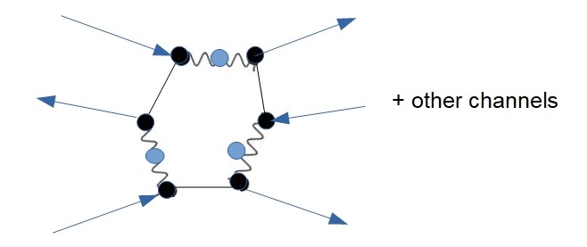
Figure 1: Three quarks/anti-quarks (solid lines) interacting by dressed gluon (wiggly line with a dot) exchange in one loop.

The non-derivative second order terms of the expansion of the quark determinant (fourth order interactions for scalar-pseudoscalar currents) were presented in Ref. [29, 37], being treated in the zero momentum transfer and local limits, so that they provide corrections to the NJL coupling constant. For the third order terms (sixth order interactions), there are many different structures involving the different quark currents. The leading derivative couplings will be also considered below, being that further derivatives are progressively suppressed with respect to the non-derivative ones. The first group of the leading terms for the flavor U(3) contain terms with at least one scalar or pseudoscalar quark current. In the local limit within zero momentum exchange and in the zero order derivative expansion, can be written as:

$${\cal L}_{6,sb,S-PS} = G_{sb,ps}T^{ijk}(J_{i}^{S}J_{j}^{PS}J_{k}^{PS}+J_{i}^{PS}J_{j}^{PS}J_{k}^{S}+J_{i}^{PS}J_{j}^{S}J_{k}^{PS})-\;G_{sb,s}T^{ijk}J_{i}^{S}J_{j}^{S}J_{k}^{S},$$ (4)

$${\cal L}_{6,sb,SVV} = T^{ijk}\left[3\;G_{sb1}J^{\mu}_{V,i}J_{\mu}^{V,j}J_{S,k}+3\;G_{sb2}J^{\mu}_{A,i}J_{\mu}^{A,j}J_{S,k}-i3\;G_{sb1}\left(J^{\mu}_{V,i}J_{\mu}^{A,j}J_{PS,k}-iJ^{\mu}_{A,i}J_{\mu}^{V,j}J_{PS,k}\right)\right],$$ (5)

$${\cal L}_{6d,SSV} = T^{ijk}\left[3\;i\;G_{d1}\;\partial_{\mu}\left(J^{\mu}_{V,i}J_{S}^{j}J_{S,k}\right)-3\;G_{d1}\left((\partial_{\mu}J^{\mu}_{A,i})J_{S,j}J^{PS}_{k}-J^{\mu}_{A,i}\left(\partial_{\mu}J^{PS}_{j}J_{S,k}\right)\right)\right]$$

$$+ T^{ijk}3\;G_{d2}\left[-J^{PS}_{i}J^{\mu}_{A,j}(\partial_{\mu}J_{S,k})+(\partial_{\mu}J^{\mu}_{A,i})J^{PS}_{j}J_{S,k}+J_{S,i}(\partial_{\mu}J_{PS,j})J_{A,k}^{\mu}-J^{\mu}_{A,i}J^{PS}_{j}(\partial_{\mu}J_{S,k})\right]$$

$$- T^{ijk}\left[-3\;i\;G_{d1}J^{\mu}_{V,i}J_{PS,j}\left(\partial_{\mu}J_{PS,k}\right)-3\;i\;G_{d2}\left(\partial_{\mu}J^{\mu}_{V,i}\right)J_{PS,j}J_{PS,k}-3\;i\;G_{d2}J^{\mu}_{V,i}\left(\partial_{\mu}J_{PS,j}\right)J_{PS,k}\right],,$$

$${\cal L}_{6,SVA,sb} = 3\;G_{sva,sb}T^{ijk}\epsilon_{\mu\nu\rho\sigma}\left[(\partial^{\mu}J_{V,i}^{\nu})(\partial^{\rho}J_{A,j}^{\sigma})J_{S}^{k}+(\partial^{\mu}J_{V,i}^{\nu})J_{S}^{j}(\partial^{\rho}J_{A,k}^{\sigma})-(\partial^{\mu}J_{V,i}^{\nu})J_{A,j}^{\sigma}(\partial^{\rho}J_{S}^{k})\right.$$ (7)

$$+ \left.(\partial^{\mu}J_{V,i}^{\nu})(\partial^{\rho}J_{S}^{j})J_{A,k}^{\sigma}-J_{V,i}^{\nu}(\partial^{\mu}J_{A,j}^{\sigma})(\partial^{\rho}J_{S}^{k})-J_{V,i}^{\nu}(\partial^{\rho}J_{S}^{j})(\partial^{\mu}J_{A,k}^{\sigma})\right],$$

where the flavor structure was written in terms of the symmetric and antisymmetric SU(3) structure constants

$$T^{ijk}=2(d_{ijk}+if_{ijk}),$$

being that the symmetric $d_{ijk}$ is directly extensible to $U(3)$. In the last line $\epsilon_{\mu\nu\rho\sigma}$ is the Levi-Civita antisymmetric tensor. The following flavor dependent coupling constants were defined, for the limit of zero momentum exchange:

$$G_{sb,s}T_{ijk} = \frac{8N_{c}}{3}K_{0}^{3}\;Tr_{D}\;Tr_{F}\int_{k}S_{0}(k)\lambda_{i}R(-k)S_{0}(k)\lambda_{j}R(k)S_{0}(k)\lambda_{k}R(-k),$$

$$G_{sb,ps}T_{ijk} = \frac{8N_{c}}{3}K_{0}^{3}\;Tr_{D}\;Tr_{F}\int_{k}S_{0}(k)i\gamma_{5}\lambda_{i}R(k)S_{0}(k)i\gamma_{5}\lambda_{j}R(k)S_{0}(k)\lambda_{k}R(-k),$$

$$G_{sb1}T_{ijk} = g^{\mu\rho}\frac{2N_{c}}{3}K_{0}^{3}Tr_{D,F}\int_{k}{S}_{0}(k)\gamma^{\nu}\lambda_{i}R_{\mu\nu}(-k){S}_{0}(k)\gamma^{\sigma}\lambda_{j}R_{\rho\sigma}(-k){S}_{0}(k)\lambda_{k}R(k),$$

$$G_{sb2}T_{ijk} = g^{\mu\rho}\frac{2N_{c}}{3}K_{0}^{3}Tr_{D,F}\int_{k}{S}_{0}(k)\gamma^{\nu}\gamma_{5}\lambda_{i}R_{\mu\nu}(-k){S}_{0}(k)\gamma^{\sigma}\gamma_{5}\lambda_{j}R_{\rho\sigma}(-k){S}_{0}(k)\lambda_{k}R(k),$$

$$G_{d1}T_{ijk} = g^{\mu\rho}\frac{4N_{c}}{3}K_{0}^{3}Tr_{D,F}\int_{k}\tilde{S}_{0}(k)\gamma_{\rho}\gamma^{\nu}\lambda_{i}R_{\mu\nu}(-k){S}_{0}(k)\lambda_{j}R(-k){S}_{0}(k)\lambda_{k}R(k),$$

$$G_{d2}T_{ijk} = g^{\mu\rho}\frac{4N_{c}}{3}K_{0}^{3}Tr_{D,F}\int_{k}{S}_{0}(k)\gamma^{\nu}\gamma_{5}\lambda_{i}R_{\mu\nu}(-k){S}_{0}(k)i\gamma_{5}\lambda_{j}R(-k)\tilde{S}_{0}(k)\gamma_{\rho}\lambda_{k}R(k),$$

$$G_{sva,sb}T_{ijk} = -\frac{\epsilon_{\rho_{1}\mu\rho_{2}\sigma}}{24}\frac{2N_{c}}{3}K_{0}^{3}\;Tr_{D,F}\int_{k}\tilde{S}_{0}\gamma^{\rho_{1}}\gamma_{\nu}\lambda_{i}R^{\mu\nu}(k)\tilde{S}_{0}\gamma^{\rho_{2}}\gamma_{\rho}\lambda_{j}R^{\rho\sigma}(-k){S}_{0}i\gamma_{5}\lambda_{k}R(-k),$$ (8)

where $Tr_{D,F}$ stands for the traces in Dirac and Flavor indices. Those coupling constants with an index including _sb are directly proportional to the quark mass, therefore corresponding to (chiral) symmetry breaking. The effective constituent quark mass will be considered to be constant, and this lead to some simplification in the analysis. All the other coupling constants, that do not include this index, are non-zero even in the case of massless quarks. The last coupling ${\cal L}_{6,SVA,sb}$, with $G_{sva,sb}$, is an anomalous interaction of a scalar current coupled to vector and axial currents.

Further leading sixth order $U_{A}(1)$ symmetry breaking quark interactions involve only vector and axial currents and at least one derivative, that, in the local limit for zero momentum exchange, are given by:

$${\cal L}_{6v1} = -3\;T_{ijk}E^{\lambda\nu\sigma\beta}\left\{G_{v1}(\partial_{\lambda}J_{V,\nu}^{i})J_{A,\sigma}^{j}J_{V,\beta}^{k}+G_{v2}\left[(\partial_{\lambda}J_{V,\nu}^{i})J_{V,\sigma}^{i}J_{A,\beta}^{k}-(\partial_{\lambda}J_{A,\nu}^{i})J_{V,\sigma}^{j}J_{V,\beta}^{k}\right]\right\}$$ (9)

$$- 3\;G_{v2}T_{ijk}\;\Gamma^{\lambda\nu\sigma\beta}\;(\partial_{\lambda}J_{V,\nu}^{i})J_{V,\sigma}^{j}J_{V,\beta}^{k}-3T^{ijk}E^{\lambda\nu\sigma\beta}\;G_{v2}(\partial_{\lambda}J_{A,\nu}^{i})J_{A,\sigma}^{j}J_{A,\beta}^{k}$$

$$- 3\;\Gamma^{\nu\sigma\lambda\beta}T^{ijk}\left[-G_{v1}J_{A,\nu}^{i}J_{A,\sigma}^{j}(\partial_{\lambda}J_{V,\beta}^{k})+G_{v2}J_{A,\nu}^{i}(\partial_{\lambda}J_{A,\sigma}^{j})J_{V,\beta}^{k}-G_{v1}(\partial_{\lambda}J_{A,i}^{\nu})J_{A,j}^{\sigma}J_{V,k}^{\beta}\right].$$

To write down a compact form for these coupling constants the gluon propagator was written in terms of a generic tensor $R^{\mu\nu}(k)=\epsilon^{\mu\nu}\bar{R}(-k)$ for which $\epsilon^{\mu\nu}=g^{\mu\nu}$ for the longitudinal component and $\epsilon^{\mu\nu}=(g^{\mu\nu}-k^{\mu}k^{\nu}/k^{2})$ for the transversal one. The following tensors were defined:

$$T^{ijk} = 2(d_{ijk}+if_{ijk}),$$ (10)

$$\Gamma^{\lambda\nu\sigma\beta} = \left(g^{\lambda\mu}g^{\rho\alpha}-g^{\lambda\rho}g^{\mu\alpha}+g^{\lambda\alpha}g^{\mu\rho}\right)\epsilon_{\mu}^{\nu}\epsilon_{\rho}^{\sigma}\epsilon_{\alpha}^{\beta},$$ (11)

$$E^{\lambda\nu\sigma\beta} = \epsilon^{\lambda\mu\rho\alpha}\epsilon_{\mu}^{\nu}\epsilon_{\rho}^{\sigma}\epsilon_{\alpha}^{\beta}.$$ (12)

The coupling constants, calculated in the zero momentum exchange limit are the following:

$$G_{v1}T_{ijk}\Gamma^{\lambda\nu\sigma\beta} = \frac{2N_{c}}{3}K_{0}^{3}Tr_{D,F}\int_{k}\gamma^{\lambda}\gamma_{\mu}\lambda_{i}\tilde{S}_{0}(k)R^{\mu\nu}(-k)\gamma_{\rho}\gamma_{5}\lambda_{j}{S}_{0}(k)R^{\rho\sigma}(-k)\gamma_{\alpha}\lambda_{k}{S}_{0}(k)R^{\alpha\beta}(k),$$ (13)

$$G_{v2}T_{ijk}\Gamma^{\lambda\nu\sigma\beta} = \frac{2N_{c}}{3}K_{0}^{3}Tr_{D,F}\int_{k}\gamma^{\lambda}\gamma_{\mu}\gamma_{5}\lambda_{i}\tilde{S}_{0}(k)R^{\mu\nu}(-k)\gamma_{\rho}\lambda_{j}{S}_{0}(k)R^{\rho\sigma}(-k)\gamma_{\alpha}\lambda_{k}{S}_{0}(k)R^{\alpha\beta}(k),$$

These three coupling constants do not vanish in the limit of zero quark masses. Also, these coupling constants may have different values for each of the flavor channel ($T_{ijk}$) if quarks are non-degenerate in the same way it has been done for the fourth order interactions [29, 37]. In this case, one must add the indices ^(ijk). The non zero momentum exchange case is straightforwardly obtained either from the expansion of the determinant - provided all the possible ordering of currents are considered.

2.1 The effective gluon propagator and renormalization condition

The effective gluon propagator to be considered in the integrals above may take into account a momentum dependent quark-gluon running coupling constant. Nevertheless, it may be needed to incorporate the corresponding renormalization constants and corresponding parameters. The following shape of (transversal) gluon effective propagator extracted from calculations with Schwinger Dyson equations at the rainbow ladder level, will be considered [38]:

$$R_{T}(k) = \frac{8\pi^{2}}{\omega^{4}}De^{-k^{2}/\omega^{2}}+\frac{8\pi^{2}\gamma_{m}E(k^{2})}{\ln\left[\tau+(1+k^{2}/\Lambda^{2}_{QCD})^{2}\right]},$$ (14)

with the following parameters $\gamma_{m}=12/(33-2N_{f})$, $N_{f}=4$, $\Lambda_{QCD}=0.234$GeV, $\tau=e^{2}-1$, $E(k^{2})=[1-exp(-k^{2}/[4m_{t}^{2}])/k^{2}$, $m_{t}=0.5GeV$, $\omega=0.5$GeV and $D=(0.55)^{3}/\omega$ (GeV²).

All the consequences of the interactions above will be discussed for their local limit and zero momentum exchange so that those interactions will be seen as corrections to the NJL-model. The gluon propagator normalization, and the overall constituent (dressed) quark current term normalization, was fixed such that the above one loop quark-antiquark interaction is the same as used in [29]. This means that the normalized fourth order flavor-dependent corrections for the NJL -coupling constants, $G_{ij}$, is reproduced for:

$$\frac{G_{11}^{NJL}}{G_{0}}\simeq 1.0.$$ (15)

3 Some consequences

All the coupling constants defined above are UV finite and break $U_{A}(1)$. They are, as a matter of fact, form factors or coupling functions that will be analyzed in the zero momentum exchange limit. Some coupling constants have dimension $M^{-5}$ (where $M$ is a mass dimension scale): $G_{sb,ps},G_{6sb2}$ and $G_{sb,s},G_{6sb1}$. The coupling constants, of one single derivative couplings, have dimension $M^{-6}$: $G_{d1},G_{d2},G_{v1}$ and $G_{v2}$. The $G_{sva,sb}$ coupling constant has dimension $M^{-7}$.

Ratios of coupling constants provide a comparison of their relative order of magnitude and they make possible to assess possible corresponding contributions to observables. There are basically two types of coupling constants from the point of view of their momentum integrals. For the present, a constant quark effective mass is considered what makes the analysis more transparent. The following relations among the coupling constants arise in the low energy regime for constituent quark masses instead of current masses and degenerate quark masses:

$$\frac{G_{sb,ps}}{M} = -\frac{G_{sb2}}{M}=G_{d2}=\frac{G_{v2}}{2},$$ (16)

$$\frac{G_{sb,s}}{M} = \frac{G_{sb1}}{M}=G_{d1}=\frac{G_{v1}}{2}\sim 4MG_{sva,sb},$$ (17)

where the last relation of the second line is suitable for very large quark mass $M$ limit. The one single derivative couplings (with $G_{d1/d2}$ and $G_{v1/v2}$) are suppressed by a factor $1/M$ with respect to those non-derivative couplings. The anomalous coupling constant $G_{sva,sb}$ is suppressed further by $M^{2}$.

The couplings with $G_{sb,ps/s}$ for scalar and pseudoscalar currents, in Eq. (4) had already been derived in [22, 23] for flavor SU(3) and SU(2) in the limit of degenerate quark masses. These flavor U(3) coupling has the same shape as those generated by the flavor U(3) determinantal ’t Hooft interaction [4]. However, for the case of any other flavor group, $SU(N_{f})$ or $U(N_{f})$, the present method still provides a sixth order interaction whereas differently from the determinantal ’t Hooft interaction [creutz]. Consequences of the $U_{A}(1)$ breaking SU(3) ’t Hooft interaction in hadron phenomenology have been investigated extensively in NJL-type models [5, 10, 11, 39]. In this type of models, these interactions drive mixing interactions for the gap equations for the quark effective masses and for the bound state (Bethe-Salpeter) equations (BSE) with results in good agreement with lattice QCD and phenomenology. One may have an estimation of their effects by resorting to a mean field approach for the scalar current. Given that the interactions were obtained by a large quark mass, or alternatively by a large gluon effective mass, the local limit of the interactions may be considered without further conditions. In this case, one may replace the scalar quark current by the scalar quark-antiquark condensate

$$J_{s}^{k}\sim<\psi\lambda^{k}\psi>.$$

In Eqs. (4) and (5), respectively, this leads to different corrections to the NJL model and vector NJL-model coupling constants. It can be written as:

$${\cal L}_{6,sb-NJL} = \frac{G_{6,PS}^{ij}}{2}J_{i}^{PS}J_{j}^{PS}-\frac{G_{6,S}^{ij}}{2}J_{i}^{S}J_{j}^{S}+\frac{G_{6,V}^{ij}}{2}J^{\mu}_{V,i}J_{\mu}^{V,j}+\frac{G_{6,A}^{ij}}{2}J^{\mu}_{A,i}J_{\mu}^{A,j},$$ (18)

where

$$G_{6,S}^{ij} = 12\;G_{sb,s}d_{ijk}<\bar{\psi}\lambda^{k}\psi>,\;\;\;\;\;G_{6,PS}^{ij}=12\;G_{sb,ps}d_{ijk}<\bar{\psi}\lambda^{k}\psi>,$$

$$G_{6,V}^{ij} = 12\;G_{sb1}d_{ijk}<\bar{\psi}\lambda^{k}\psi>,\;\;\;\;\;\;G_{6,A}^{ij}=12\;G_{sb2}d_{ijk}<\bar{\psi}\lambda^{k}\psi>.$$ (19)

For the up, down and strange scalar quark-antiquark condensates, the components $k=0,3,8$ contribute as:

$$<\bar{\psi}\lambda_{0}\psi> = \sqrt{\frac{2}{3}}\left(<\bar{u}u>+<\bar{d}d>+<\bar{s}s>\right),$$

$$<\bar{\psi}\lambda_{3}\psi> = <\bar{u}u>-<\bar{d}d>,$$

$$<\bar{\psi}\lambda_{8}\psi> = \frac{1}{\sqrt{3}}\left(<\bar{u}u>+<\bar{d}d>-2<\bar{s}s>\right).$$ (20)

These fourth-order quark-antiquark corrections break $U_{A}(1)$. The resulting corrections for the NJL-model coupling constants must be compared to an original coupling constant $G_{0}$ for the normalization given in Eq. (15).

Numerical estimates for the coupling constants in Eqs. (2) and (13) are shown in Table (1) by considering the parameters of the fitting of the NJL given in [29] for which $G_{0}=10$ GeV^-2. The following phenomenological values of the parameters:

$$M_{u}=M_{d}=M_{s}=0.391\;\mbox{GeV}$$

$$<\bar{u}u>=<\bar{d}d>=(-0.240)^{3}\mbox{ GeV}^{3},\;\;\;\;\;<\bar{s}s>=(-0.290)^{3}\;\mbox{ GeV}^{3}.$$ (21)

In few situations where mixing coupling constants are directly dependent on quark mass differences, the partially non-degenerate quark masses were employed: $M_{u}=M_{d}=0.391$ GeV, $M_{s}=0.600$ GeV. Because of the ambiguities to define scalar and axial states to form quark-antiquark mesons nonets, numerical estimates will be provided mostly for the up and down quark sector.

Table 1: Numerical results for the resulting parameters for $T_{ijk}=2d_{11k}$ ($k=0,8$) , by using parameters Eq. (3) and effective gluon propagator (14). For the mixing parameters (*) the following masses have been used: $M_{u}=M_{d}=0.391$GeV, $M_{s}=0.600$ GeV.

	$G_{sb,s}/G_{sb,ps}$	$G_{sb1}/G_{sb2}$	$G_{d1}/G_{d2}$	$G_{v1}/G_{v2}$	$G_{sva,sb}$	$G_{6,S}^{11}$/$G_{6,PS}^{11}$	$G_{6,V}^{11}$/$G_{6,A}^{11}$
	GeV-5	GeV-5	GeV-6	GeV-6	GeV-7	GeV-2	GeV-2
$T_{118}$	2.9/86.7	2.9/-86.7	59.3/221.7	118.7/443.5	-459.7	-0.31/-9.4	-0.16/4.7
		$G_{03}^{ps}$/$G_{03}^{s}$	$G_{08}^{ps}$/$G_{08}^{s}$	$G_{38}^{ps}$/ $G_{38}^{s}$	$G_{03}^{v}$/$G_{03}^{a}$	$G_{08}^{v}$/$G_{08}^{a}$	$G_{38}^{v}$/$G_{38}^{a}$
		GeV-2	GeV-2	GeV-2	GeV-2	GeV-2	GeV-2
$T_{118}$ (*)		-0.08/-0.40	-0.79/-3.85	-0.05/-0.23	-0.06/0.28	-0.56/2.72	- 0.03/0.16

Note that, for the instanton induced ’t Hooft interaction one would have $G_{sb,s}=3G_{sb,ps}$ whereas in the polarization induced coupling constant the values for the scalar and pseudoscalar channels are different. By identifying the scalar part of the ’t Hooft interaction (with coupling constant $\kappa$) with the scalar (or pseudoscalar) part $G_{sb,s/ps}$ one has: $\kappa=-32\times G_{sb,s/ps}.$ These values presented in the Table above may therefore smaller than, or of the same order of magnitude as, different fittings for the NJL model that are in the range of $\kappa\sim-100\to-2500$ GeV^-5 [11, 40]. It is important to notice that these ’t Hooft interactions used in the NJL model as a matter of fact can include the interactions from polarization processes, at the end only a fitting for their numerical values is needed in such models. Their (mean field) contributions for the flavor dependent NJL-coupling constants, identified in Eq. (18), are denoted in the Table by $G_{6,S}^{11}/G_{6,PS}^{11}$ and their values are quite smaller than $G_{0}=10$ GeV^-2.

In spite of the different nature, the coupling constants $G_{sb1}$ and $G_{sb2}$ are vector and axial counterparts of ’t Hooft interactions - being non-derivative. At the mean field level, analogously to the scalar-pseudoscalar terms, they induce contributions for the vector-NJL coupling constants, denoted by $G_{6,V}^{11}/G_{6,A}^{11}$ that are displayed in the last entry of the first line. They also are much smaller than the typical values of the NJL model coupling constant. Being proportional to the quark chiral condensate, these coupling constants go to zero with the restoration of DChSB. Numerical values for the derivative interactions $G_{d1/d2},G_{v1/v2}$ and $G_{sva,sb}$ in the channel $T^{118}$ are also displayed. Although their numerical values are larger, they have smaller dimensions, respectively $M^{-6}$ and $M^{-7}$.

Concerning the mixing parameters $G_{i\neq j}^{\phi}$, the values obtained for the pseudoscalar/scalar mixing are of the same order of magnitude of those obtained from the second order terms of the one loop polarization approach [29] with a similar normalization point to Eq. (15). The same hierarchy of larger and smaller values are obtained, in particular for the sets of parameters $Y$ Table II of Ref. [29]:

$$G_{03}^{ps}\sim 0.03-0.11\;(GeV^{-2}),\;\;\;\;\;G_{08}^{ps}\sim 1.04-2.39\;(GeV^{-2}),\;\;\;\;\;G_{38}^{ps}\sim 0.04-0.14\;(GeV^{-2}).$$

The mixing interactions for the vector channels will be compared to other works below for the bosonized version of the interactions.

4 Corresponding mesons dynamics

By associating each of the flavor currents to a local meson field belonging to a flavor multiplet (nonet) - vector, axial, pseudoscalar and scalar-, the above sixth order interactions give rise to three-meson couplings. They can be associated to $U_{A}(1)$-breaking contributions to decay rates, although they may lead to rearrangements to meson mixing or even masses. Local meson fields can be implemented by means of the auxiliary field method with functional delta functions [41] as the following ones:

$$1 = N\int D[S_{i},P_{i}]\delta(S_{i}-G_{0,s}^{ii}J_{i})\delta(P_{i}-G_{0,p}^{ii}J_{P,i})\;\int D[V_{\mu},A_{\mu}]\delta(V^{\mu}_{i}-G_{0,v}^{ii}J_{V,i}^{\mu})\delta(A_{i}^{\mu}-G_{0,a}^{ii}J_{A,i}^{\mu}),$$ (22)

where $N$ is a normalization, $S_{i},P_{i},V_{i}^{\mu},A_{i}^{\mu}$ are the meson fields of each of the flavor multiplet, $D[S_{i},P_{i}]$ and $D[V_{\mu},A_{\mu}]$ are the measures of integration, and $G_{0,s}^{ii},G_{0,p}^{ii},G_{0,v}^{ii}$ and $G_{0,a}^{ii}$ are constant parameters with dimension $M^{-2}$, to be fixed latter. These last parameters may include the renormalization constants for each of the meson fields implicitly what is usually introduced in a more standard way with functional delta function such as the following: $\delta(\phi\sqrt{Z}_{\phi}-G_{0}^{ii}J_{i}^{\phi})$, being that $\phi$ is any of the local meson fields and $G_{0}$ is a dimensionful constant such as the NJL coupling constant [42, 43]. Because the calculation will be basically done for degenerate quark masses, the indices ⁱⁱ in $G_{0,\phi}$ will be suppressed in most part of the calculation to make notation easier to read. The fields $S_{i}$ will be referred as scalar mesons fields even if a mixing to other components (tetraquark, molecular or gluonic) may be needed.

The local limit of the Lagrangian terms above lead to the following contributions for the mesons dynamics:

$${\cal L}_{6,sb,S-PS}^{mes} = \frac{G_{sb,ps}}{G_{0,s}G_{0,ps}^{2}}T^{ijk}(S_{i}P_{j}P_{k}+P_{i}P_{j}S_{k}+P_{i}S_{j}P_{k})-\;\frac{G_{sb,s}}{G_{0,s}^{3}}T^{ijk}S_{i}S_{j}S_{k},$$ (23)

$${\cal L}_{6,sb,SVV}^{mes} = T^{ijk}\left[\frac{3\;G_{sb1}}{G_{0,s}G_{0,v}^{2}}V^{\mu}_{i}V_{\mu}^{j}S_{k}+\frac{3\;G_{sb2}}{G_{0,s}G_{0,a}^{2}}A^{\mu}_{i}A_{\mu}^{j}S_{k}-\frac{3i\;G_{sb1}\left(V^{\mu}_{i}A_{\mu}^{j}P_{k}-A^{\mu}_{i}V_{\mu}^{j}P_{k}\right)}{G_{0,v}G_{0,ps}G_{0,a}}\right],$$ (24)

$${\cal L}_{6d,SSV}^{mes} = -3\;\frac{G_{d1}}{G_{0,a}G_{0,s}G_{0,ps}}T^{ijk}\left[(\partial_{\mu}A^{\mu}_{i})S_{j}P_{k}-A^{\mu}_{i}\left(\partial_{\mu}P_{j}\right)S_{k}\right]$$

$$+ 3\;\frac{G_{d2}}{G_{0,a}G_{0,ps}G_{0,s}}T^{ijk}\left[-\partial_{\mu}\left(A^{\mu}_{i}P_{j}+P_{i}A^{\mu}_{j}\right)+(\partial_{\mu}A^{\mu}_{i})P_{j}+(\partial_{\mu}P_{j})A_{k}^{\mu}\right]\;S^{k}$$

$$- 3i\;\frac{G_{d1}}{G_{0,v}G_{0,ps}^{2}}T^{ijk}V^{\mu}_{i}P_{j}\left(\partial_{\mu}P^{k}\right)-3\;\frac{G_{d2}}{G_{0,v}G_{0,ps}^{2}}T^{ijk}\left[\left(\partial_{\mu}V^{\mu}_{i}\right)P^{j}P_{k}+V_{i}^{\mu}\left(\partial_{\mu}P_{j}\right)P^{k}\right],$$

$${\cal L}_{6,SVA,sb}^{mes} = 3\;\frac{G_{sva,sb}}{G_{0,a}G_{0,v}G_{0,s}}T^{ijk}\epsilon_{\mu\nu\rho\sigma}\left\{(\partial^{\mu}V^{\nu}_{i})(\partial^{\rho}A_{j}^{\sigma})S^{k}+(\partial^{\mu}V^{\nu}_{i})S^{j}(\partial^{\rho}A_{k}^{\sigma})-(\partial^{\mu}V^{\nu}_{i})A^{j}_{\sigma}(\partial^{\rho}S_{k})\right.$$ (26)

$$- \left.V^{\nu}_{i}(\partial^{\mu}S^{j})(\partial^{\rho}A_{k}^{\sigma})-V^{\nu}_{i}(\partial^{\rho}A_{j}^{\sigma})(\partial^{\mu}S^{k})+(\partial^{\mu}V^{\nu}_{i})(\partial^{\rho}S_{j})A^{k}_{\sigma}\right\},$$

$${\cal L}_{6v1}^{mes} = -3\;\frac{G_{v1}}{G_{0,a}G_{0,v}^{2}}T_{ijk}E^{\lambda\nu\sigma\beta}\left\{(\partial_{\lambda}V_{\nu}^{i})A_{\sigma}^{j}V_{\beta}^{k}\right\}-3\;\frac{G_{v2}}{G_{0,a}G_{0,v}^{2}}T_{ijk}E^{\lambda\nu\sigma\beta}\left\{(\partial_{\lambda}V_{\nu}^{i})V_{\sigma}^{i}A_{\beta}^{k}-(\partial_{\lambda}A_{\nu}^{i})V_{\sigma}^{j}V_{\beta}^{k}\right\}$$ (27)

$$- 3\;\frac{G_{v2}}{G_{0,v}^{3}}T_{ijk}\;\Gamma^{\lambda\nu\sigma\beta}\;(\partial_{\lambda}V_{\nu}^{i})V_{\sigma}^{j}V_{\beta}^{k}-3\;\frac{G_{v2}}{G_{0,a}^{3}}T^{ijk}E^{\lambda\nu\sigma\beta}(\partial_{\lambda}A_{\nu}^{i})A_{\sigma}^{j}A_{\beta}^{k}$$

$$+ 3\;\Gamma^{\nu\sigma\lambda\beta}T^{ijk}\left[\frac{G_{v1}}{G_{0,a}^{2}G_{0,v}}A_{\nu}^{i}A_{\sigma}^{j}(\partial_{\lambda}V_{\beta}^{k})-\frac{G_{v2}}{G_{0,a}^{2}G_{0,v}}A_{\nu}^{i}(\partial_{\lambda}A_{\sigma}^{j})V_{\beta}^{k}+\frac{G_{v1}}{G_{0,a}^{2}G_{0,v}}(\partial_{\lambda}A_{i}^{\nu})A_{j}^{\sigma}V_{k}^{\beta}\right],$$

For all of these couplings, renormalized coupling constants may be defined by incorporating the constant factors $1/G_{0,\phi}$ and the numerical coefficients, such as 3 or 6. Below, a criterion to determine these constants will be provided. These renormalized coupling constants can be written, for example, in the case of degenerate quark mass as:

$$G_{sb,ps}^{R}=\frac{G_{sb,ps}}{G_{0,s}^{3}},\;\;\;\;G_{sva,sb}^{R}=3\;\frac{G_{sva,sb}}{G_{0,v}^{2}G_{0,s}}\;\;\;\;G_{v1}^{R}=3\;\frac{G_{v1}}{G_{0,v}^{3}}\;,\;\;...$$ (28)

The following types of three-meson couplings show up in the Lagrangian above: the different scalar combinations of three scalar and pseudoscalar mesons (SSS, SPP) (23), vector-axial -pseudoscalar mesons (VPA) with $G_{sb1}$ and $G_{sb2}$ (24), one scalar with two vector or two axial mesons (SVV, SAA) (24), momentum dependent vector meson-two pseudoscalar mesons (VPP), or scalar-axial-pseudoscalar mesons - ASP, in (4), momentum dependent combinations of three vector/axial mesons (VVV,AAA) $G_{v1},G_{v2}$ (27), and the anomalous (SVA) $G_{sva,sb}$ (26). The scalar current may represent a medium with finite baryonic density and, in the anomalous coupling $G_{sva,sb}$, it is needed to conserve linear momentum. This interaction has been already presented in [PRD-2022a] and below it is treated within a different renormalization. Other interactions appear for higher order in the derivative whose coupling constants are, however, still weaker. The (derivative) vector and axial mesons couplings may be part of (global) gauge invariant couplings as presented, for example, in [44] whose complete analysis is outside the scope of this work. It will be enough to restrict the resulting terms from the expansion for the Abelian stress tensors, that are defined as $V_{\mu}=V_{\mu}^{i}\cdot\lambda^{i}$, by

$${\cal F}_{\mu\nu}^{i}=\partial_{\mu}V_{\nu}^{i}-\partial_{\nu}V_{\mu}^{i},\;\;\;\;\;\;\;{\cal G}_{\mu\nu}=\partial_{\mu}A_{\nu}^{i}-\partial_{\nu}A_{\mu}^{i}.$$

Their complete contributions however will not be explored in the present work.

4.1 Parameters $G_{0,\phi}$: renormalization conditions

The meson kinetic terms, generated by the expansion of the determinant, will be used as renormalization conditions to determine the parameters $G_{0,\phi}$ for $\phi=S,P,V,A$ as proposed in [42]. The free meson kinetic terms arise, and they provide basically the full meson normalization constants. The resulting meson kinetic terms, with the Abelian vector and axial mesons stress tensors, are given by [42, 27]:

$${\cal L}_{mass} = \frac{1}{2}\frac{I_{0,S}^{ii}}{(G_{0,S}^{ii})^{2}}\partial_{\mu}S_{i}\partial^{\mu}S_{i}+\frac{1}{2}\frac{I_{0,S}^{ii}}{(G_{0,P}^{ii})^{2}}\partial_{\mu}P_{i}\partial^{\mu}P_{i}-\frac{1}{8}\frac{I_{0,V}^{ii}}{(G_{0,v}^{ii})^{2}}{\cal F}_{i}^{\mu\nu}{\cal F}_{\mu\nu}^{i}-\frac{1}{8}\frac{I_{0,A}^{ii}}{(G_{0,a}^{ii})^{2}}{\cal G}_{i}^{\mu\nu}{\cal G}_{\mu\nu}^{i}$$ (29)

$$= \frac{1}{2}\partial_{\mu}S_{i}\partial^{\mu}S_{i}+\frac{1}{2}\partial_{\mu}P_{i}\partial^{\mu}P_{i}-\frac{1}{4}{\cal F}_{i}^{\mu\nu}{\cal F}_{\mu\nu}^{i}-\frac{1}{4}{\cal G}_{i}^{\mu\nu}{\cal G}_{\mu\nu}^{i}$$

Written in this way it is direct the association of the parameters $G_{0,\phi}$ to the renormalization constants of the corresponding fields. Therefore, it follows:

$$G_{0,S}^{i}=\sqrt{I_{0,S}^{ii}} = G_{0,P}^{i}=\sqrt{I_{0,P}^{ii}},$$

$$G_{0,V}^{i}=\sqrt{I_{0,V}^{ii}/2}, = G_{0,A}^{i}=\sqrt{I_{0,A}^{ii}/2}.$$ (30)

These parameters provide renormalized expressions for the three-meson coupling constants shown above.

4.2 Estimation of $U_{A}(1)$ breaking contributions for the Mesons Masses and mixings

Meson masses can be computed by solving Bethe-Salpeter Equation (BSE) that may also be done as usually done in NJL or other approach [10, 11, 38]. By expanding the resulting Lagrangian terms that generate the corresponding BSE one can write down effective Lagrangian terms for the masses of such mesons obtained from the BSE. To provide an estimation, one can add to these effective Lagrangian terms, the corrections obtained from the 6th order terms above. By adopting a mean field value for the scalar current as done above for the quark currents, it can be written as the scalar chiral condensate, $\frac{S_{j}}{G_{0,s}}=<\bar{\psi}\lambda_{j}\psi>$. In this case, meson fields can be considered as parts of U(3) flavor-nonets. In this mean field approach one can write the corresponding effective contributions for the mass terms as:

$$\Delta{\cal L}_{S-PS} = -\frac{(\Delta^{ps}M_{ji}^{2})}{2}P_{j}P_{k}-\frac{(\Delta^{s}M_{ji}^{2})}{2}S_{j}S_{k},\;\;\;\;\;\;\mbox{from}\;\;\;\;{\cal L}_{6,sb,S-PS}.$$ (31)

$${\cal L}_{V-A} = -\frac{(\Delta^{V}M^{2}_{ji})}{2}V^{\mu}_{i}V_{\mu}^{j}-\frac{(\Delta^{A}M_{ji}^{2})}{2}A^{\mu}_{i}A_{\mu}^{j},\;\;\;\;\;\;\mbox{from}\;\;\;\;{\cal L}_{6,sb,SVV},$$ (32)

where these mass corrections are the following

$$(\Delta^{ps}M_{ji}^{2}) = -12d_{jik}\frac{{G}_{sb,ps}}{G_{0,ps}^{2}}<\bar{\psi}\lambda_{k}\psi>,\;\;\;\;\;(\Delta^{s}M_{ji}^{2})=12d_{jik}\frac{{G}_{sb,s}}{G_{0,s}^{2}}<\bar{\psi}\lambda_{k}\psi>,$$

$$(\Delta^{v}M_{ji}^{2}) = 12d_{jik}\frac{{G}_{sb1}}{G_{0,v}^{2}}<\bar{\psi}\lambda_{k}\psi>,\;\;\;\;\;(\Delta^{a}M_{ji}^{2})=12d_{jik}\frac{{G}_{sb2}}{G_{0,a}^{2}}<\bar{\psi}\lambda_{k}\psi>.$$ (33)

Some of these contributions will be calculated below, namely the ones for the lightest mesons of each multiplet: the charged pion and kaon masses and corresponding scalar meson states $a_{0}(980),K_{0}^{*}(650-800$ respectively for $i=1,2$ and $i=4,5$ [45, 37], for the charged vector $\rho(770)$ and $K^{*}(892)$ masses and corresponding axial mesons $A_{1}(1260),K_{1}(1270)$ also respectively for $i=1,2$ and $i=4,5$ [45]. The mass parameters $\Delta^{\phi}M_{ij}^{2}$ in Eqs. (31) and (32) were written in such a way to identify also mixing terms for $i\neq j$. The scalar/pseudoscalar mixing were compared to other available results above at the level of quark currents. For the vector channel, consider the possible mixings between the components $\phi_{0},\phi_{3},\phi_{8}$ of each of the meson multiplet, can be denoted by $G_{0,3}^{\phi},G_{08}^{\phi}$ and $G_{3,8}^{\phi}$ can be written as:

$$G_{0,3}^{R,v/a}\equiv\;-\frac{(\Delta^{v/a}M_{03}^{2})}{2} = -12\;d_{033}\frac{{G}_{sb,v/a}}{G_{0,v/a}^{2}}<\bar{\psi}\lambda_{3}\psi>,$$

$$G_{0,8}^{R,v/a}\equiv-\frac{(\Delta^{v/a}M_{08}^{2})}{2} = -12\;d_{088}\frac{{G}_{sb,v/a}}{G_{0,v/a}^{2}}<\bar{\psi}\lambda_{8}\psi>,$$

$$G_{3,8}^{R,v/a}\equiv-\frac{(\Delta^{v/a}M_{38}^{2})}{2} = -12\;d_{338}\frac{{G}_{sb,v/a}}{G_{0,v/a}^{2}}<\bar{\psi}\lambda_{3}\psi>.$$ (34)

In each of the mesons flavor U(3) multiplets under analysis [46], pseudoscalar, scalar, vector and axial channels, the following neutral meson mixings arise:

$$\pi^{0}-\eta-\eta^{\prime},\;\;\;\;\;\rho^{0}-\omega-\phi,\;\;\;\;\;a_{1}^{0}(1260)-f_{1}(1280)-f_{1S}(1420)$$

and the controversial case of the light scalars for which the quark-antiquark components may contribute for $\sigma(500)-a_{0}^{0}(980)-f_{0}(980)$ [45, 30, 31] In the pseudoscalar sector, a mixing coupling between pion-kaon, in such mean field for eqs. (31) with $G_{sb,ps}^{ijk}$, is forbidden since it would not conserve strangeness or isospin. This is seen in the absence of symmetric structure constants that relate $i=1,2,3$ and $i=4,5,6,7$. Results for the three-leg coupling constants and contributions for masses and mixing parameters are presented in the Table (2).

Table 2: Some numerical results for the (renormalized) parameters in the meson sector by using parameters Eq. (3) and effective gluon propagator (14). For the mixing parameters (*) the following masses have been used: $M_{u}=0.35$GeV, $M_{d}=0.355$GeV, $M_{s}=0.65$ GeV.

	$G_{sb,ps}^{R}$	$G_{sb,s}^{R}$	$G_{sb1}^{R}$	$G_{sb2}^{R}$	$G_{d1}^{R}$	$G_{d2}^{R}$	$G_{v1}^{R}$	$G_{v2}^{R}$
	GeV	GeV	GeV	GeV	-	-	-	-
$T_{118}$	0.013	0.004	0.019	0.071	0.182	0.049	0.514	0.138
	$\Delta M_{\pi}^{2}$	$\Delta M_{K}^{2}$	$\Delta M_{A_{0}}^{2}$	$\Delta M_{K_{0}^{*}}^{2}$	$\Delta M_{\rho^{\pm}}^{2}$	$\Delta M_{{K^{*}}^{\pm}}^{2}$	$\Delta M_{A_{1}^{\pm}}^{2}$	$\Delta M_{K_{1}^{\pm}}^{2}$
	(i=1,2)	(i= 4,5)	(i=1,2)	(i= 4,5)	(i=1,2)	(i= 4,5)	(i=1,2)	(i= 4,5)
	GeV2	GeV2	GeV2	GeV2	GeV2	GeV2	GeV2	GeV2
	$9.9\times 10^{-4}$	$-12.6\times 10^{-4}$	$3.7\times 10^{-3}$	$-4.7\times 10^{-3}$	0.004	- 0.005	0.015	-0.019
		$G_{03}^{R,ps}$/$G_{03}^{R,s}$	$G_{08}^{R,ps}$/$G_{08}^{R,s}$	$G_{38}^{R,ps}$/ $G_{38}^{R,s}$	$G_{03}^{R,v}$/$G_{03}^{R,a}$	$G_{08}^{R,v}$/$G_{08}^{R,a}$	$G_{38}^{R,v}$/$G_{38}^{R,a}$
		GeV2	GeV2	GeV2	GeV2	GeV2	GeV2
(*)		-0.06/-1.78	-0.58/-17.33	-0.03/-1.03	-0.06/1.78	-0.58/17.33	- 0.02/1.03

The couplings $SSS$ and $SPP$ correspond to similar structures of the bosonized ’t Hooft interaction as discussed above, for which the following (flavor-independent) relation holds: $G_{sb,ps}^{tHooft}=3G_{sb,s}^{tHooft}$, that is different from the obtained above.

The coupling $V-P-A$ in ${\cal L}_{sb,SVV}^{mes}$ with $G_{sb1/2}^{R}$ corresponds to vector-pseudoscalar-axial mesons vertex whose phenomenological values in the literature are one order of magnitude larger than the ones present in the Table. For example, in Ref. [47] the vertex $\pi-\rho-A_{1}$ was found to be: $G_{v-a-\pi}\sim 2M\sim 0.7\;\mbox{GeV}$. A similar estimate to the present work was done in [27], for a different (re)normalization, that is $G_{A\pi V}\sim 0.7-1.2$. The coupling constants $G_{sb1/2}^{R}$ also drives couplings of the type $V-V-S$ and $A-A-S$ discussed above.

The couplings $V-P-P$ in ${\cal L}_{sb,SVV}^{mes}$ with $G_{d1/d2}^{R}$ stand for vector meson - two pseudoscalar mesons. These coupling constants also drive axial-pseudoscalar-scalar mesons vertices ($A-S-P$). For the lightest quark sector it corresponds to the vertex $\rho-\pi-\pi$ such that $G_{\rho-\pi-\pi}=3(G_{d1}^{R}\pm G_{d2}^{R})$ for which there are several estimates in the literature that are of the order of magnitude of the values presented in the Table (2). For instance, from [45]: $G_{\rho-\pi\pi}=\sqrt{4\;\pi\;2.9}\sim 6$.

The numerical values of the quantities $\Delta M_{\phi}^{2}$ provide a naif estimation of the effects of the corresponding interactions on the meson mass. Although meson masses are obtained by solving the corresponding BSE, these terms may be taken as corrections to the effective action with the physical meson masses previously calculated with the corresponding BSE. These BSE are the ones previously solved with the same parameters considered in this work from [29]. However, the relative magnitude and the corresponding sign can indicate which mesons would receive larger contributions from this term, with the relative sign that may be positive or negative. For the charged meson states built up with flavor generators $\lambda_{1},\lambda_{2}$ ($\lambda_{4},\lambda_{5}$, therefore with one strange quark or antiquark) the contribution of this quadratic term is positive (negative).

The scalar-pseudoscalar meson mixings ($G_{i\neq j}^{R,ps}/G_{i\neq j}^{R,s}$) are of the same order of magnitude of those derived and investigated in [29, 37, 31], although a different procedure for the overall normalization have been considered. The vector mesons mixings ($G_{i\neq j}^{R,v}$) are one order of magnitude larger than results presented in the literature [48]. However, the hierarchy is the same, i.e. the rho-omega mixing ($G_{03}^{R}$) is one order of magnitude smaller than the omega-phi mixing $G_{08}^{R}$). The rho-phi mixing ($G_{38}^{R}$) is the smallest one. The axial meson mixings ($G_{i\neq j}^{R,a}$) are not well established, being these mesons very unstable.

Several of the three mesons couplings, shown above, in the adopted mean field approach, represent corrections to not only the controversial so-called pion- axial meson mixing, $\pi-A_{1}$, coupling [49], but also correspondingly kaon-axial meson $K-K_{1}$ mixing and others, being all momentum dependent couplings. These couplings were already presented for the fourth order terms of the quark determinant expansion in [27]. By adopting the mean field approach for the scalar currents, the following mixings are found:

$${\cal L}_{6d,SSV-mes} = G_{A-P}^{R,(ij)}\left[(\partial_{\mu}A^{\mu}_{i})P_{j}-A^{\mu}_{j}\left(\partial_{\mu}P_{i}\right)\right],\;\;\;\;\;\;\;\;G_{A-P}^{R,(ij)}=-6\;d^{ijk}\frac{G_{d1}}{G_{0,a}G_{0,ps}}<\bar{\psi}\lambda^{k}\psi>,$$ (35)

For the case of the lighter mesons $ij=1,2,3$, pions and $A_{1}$, one has the values of the Table for $G_{d1},G_{d2}$. The following value is found:

$$G_{A_{1}-\pi}^{R},\simeq 0.17\;\mbox{GeV}.$$ (36)

The $\pi-A_{1}$ mixing is usually eliminated by a redefinition of the axial meson field such as $A_{\mu}\to A_{\mu}+K\partial_{\mu}P$. If a field redefinition of the $A_{1}$ meson field is performed to eliminate such mixing in the second order mixing term [50], the mixings above (35) - of third order - still survive. So the mixing should have to be done order by order in the determinant expansion. It seems that this coupling will not be eliminated consistently in all orders by a single field redefinition of the A1. However, a complete proof did not seem possible so far. Otherwise, by trying to do the field redefinition in the quark determinant before expansion, the derivative couplings of the pion would disappear.

The third order correction to the anomalous coupling $G_{sva,sb}^{R}$ can be associated to a highly momentum dependent vector meson-axial meson mixing in the presence of a quark scalar current, scalar meson or finite density medium. As discussed in [27], for the second order coupling, this anomalous vector-axial mixing it is strongly dependent on the mesons polarizations and it can only take place close to a third particle or in a medium to make possible the conservation of momentum, since axial and vector mesons momenta must be transverse to each other. It has been argued in that work that it makes possible to probe the axial constituent quark (baryon) current or charge by means of vector mesons. It can be written for the mean field level:

$${\cal L}_{6,SVA,sb} = G_{A-V}^{R,(ij)}\;\epsilon_{\mu\nu\rho\sigma}(\partial^{\mu}V^{\nu}_{i})(\partial^{\rho}A_{j}^{\sigma}),\;\;\;\;\;\;\;G_{A-V}^{R,(ij)}=8d^{ijk}\;\frac{G_{sva,sb}}{G_{0,a}G_{0,v}}<\bar{\psi}\lambda^{k}\psi>,$$ (37)

For the case of the lighter mesons $ij=1,2,3$ for the $\rho^{0}$ and axial $A_{1}$ one has the values of the Table that yields

$$G_{A_{1}-\rho}^{R,(11)}\simeq-0.07.$$ (38)

This (dimensionless) value is quite smaller than the others and it must be difficult to be observed experimentally because the axial mesons are quite unstable and the final state is strongly interacting. This type of mixing has been considered in many situations for finite (energy/baryonic) densities including in heavy ion collisions [33, 34] being therefore proportional to the baryonic density as $\xi_{\rho-A_{1}}=C_{V-A}(\rho_{N})/\rho_{0}$ where $C_{V-A}\sim 0.3$.

5 Summary

Sixth order $U_{A}(1)-$ breaking quark interactions were obtained in the large quark mass expansion of the quark determinant in the presence of background (constituent) quark currents. The corresponding local limit was analyzed. Four types of quark currents were considered: scalar, pseudoscalar, vector and axial ones. For the case of non-degenerate quark masses, all the coupling constants, as the limit of zero momentum transfer, break flavor symmetry. These resulting effective interactions are of the order of $\alpha^{2n}_{s}$, $n=3$, where $\alpha_{s}$ is the quark-gluon running coupling constants. In energies lower than the dynamical chiral symmetry restoration, the effective coupling constants depend on the quark effective masses. For energies around and above the restoration of Dynamical Chiral Symmetry Breaking [51], besides thermal effects, the running quark-gluon coupling constant is considerably weaker and quark masses reduce to the current quark masses [45], although they should not vanish [2]. Therefore, the strength of such sixth order quark-antiquark interactions may decrease drastically, in particular for those interactions proportional to quark masses, labeled by _sb. However, they may not disappear, in agreement with [26, 12]. By resorting to a mean field approach to the scalar quark currents in the local limit of the interactions, several sixth order interactions reduce to fourth order interactions which make possible to exploit some phenomenological consequences in terms of the parameters of a NJL-model with the corresponding dynamics.

By employing the auxiliary field method, the quark-current interactions were rewritten as three-leg meson vertices that were investigated in the local limit. The limit of zero momentum exchange adopted in these estimations provide an upper bound for the resulting three-meson running coupling constants. Some coupling constants were estimated and compared to other works, showing a reasonably good agreement for the order of magnitude. All the vertices contain the overall structure from both the symmetric and the asymmetric flavor structure constants, although in some cases only one or the other may contribute. Although these three-meson leg vertices are associated to meson decays, the investigation of decay rates were left outside the scope of this work and will be presented in a forthcoming work.

Acknowledgements

The author thanks a short conversation with T. Kovács. F.L.B. is a member of INCT-FNA, Proc. 464898/2014-5 and he acknowledges partial support from CNPq-312750/2021 and CNPq-407162/2023-2.

References

• [1] S. L. Adler, Phys. Rev. 177, 2426 (1969); J. Bell and R. Jackiw, Nuovo Cimento A 60, 47 (1969). K. Fujikawa, Phys. Rev. Lett. 42, 1195 (1979).
• [2] M. Creutz, Anomalies and chiral symmetry in QCD, Annals of Physics 324, 1573 (2009).
• [3] K. Fujikawa, Path-integral measure for gauge-invariant fermion theories, Phys. Rev. Lett. 42 (1979) 1195.
• [4] G. ’t Hooft, Computation of the quantum effects due to a four-dimensional pseudoparticle, Phys. Rev. D 14, 3432 (1976); Erratum: ibid D 18, 2199 (1978).
• [5] E. Witten, Instantons, the quark model, and the 1/N expansion, Nucl. Phys. B149, 285 (1979).
• [6] F. Giacosa, A. Koenigstein, R.D. Pisarski, How the axial anomaly controls flavor mixing among mesons, Phys. Rev. D97, 091901(R) (2018).
• [7] E. Witten, Baryons in the 1/$N_{c}$ expansion, Nucl. Phys. B160, 57 (1979).
• [8] E. Witten, Large N chiral dynamics, Ann. Phys. 128, 363 (1980).
• [9] R. D. Pisarski and F. Wilczek, Remarks on the chiral phase transition in chromodynamics, Phys. Rev. D 29, 338 (1984).
• [10] Y. Nambu, G. Jona-Lasinio, Dynamical Model of Elementary Particles Based on an Analogy with Superconductivity I, Phys. Rev. 122, 345 (1961).
• [11] U. Vogl, W. Weise, The Nambu and Jona-Lasinio model: Its implications for Hadrons and Nuclei, Progr. in Part. and Nucl. Phys. 27, 195 (1991). S. Klimt, M. Lutz, U. Vogl, W. Weise, Generalized SU(3) Nambu-Jona-Lasinio model. Nucl. Phys. A 516, 429 (1990). S. P. Klevansky The Nambu-Jona-Lasinio model of quantum chromodynamics, Rev. Mod. Phys. 64, 649 (1992).
• [12] R. D. Pisarski and F. Rennecke, The chiral phase transition and the axial anomaly 2401.06130v2 [hep-ph].
• [13] For example: P. Kovacs, Zs. Szep, and Gy. Wolf, Phys. Rev. D93, 114014 (2016). A. Gomez Nicola and J. Ruiz de Elvira, Phys. Rev. D98, 014020 (2018). X. Li, W.-J. Fu, and Y.-X. Liu, Phys. Rev. D101, 054034 (2020). F. Fejos, A. Patkos, Thermal behavior of effective $U_{A}(1)$ anomaly couplings in reflection of higher topological sectors, arXiv:hep-ph: 2311.02186
• [14] C. Rosenzweig, J. Schechter, C.G. Trahern, Is the effective Lagrangian for quantum chromodynamics a sigma model?, Phys. Rev. D 21 (1980) 3388; R.L. Arnowitt, P. Nath, Nucl. Phys. B 209 (1982) 234; K. Kawarabayashi, N. Ohta, Prog. Theor. Phys. 66 (1981) 1408; N. Ohta, Prog. Theor. Phys. 66 (1981) 1789; P. Nath, R.L. Arnowitt, U(1) problem: Current algebra and the theta vacuum, Nucl. Phys. B 209 (1982) 251. D. Boer, J.K. Boomsma, Phys. Rev. D 78 (2008) 054027 (arXiv:0806.1669 [hep-ph]).
• [15] F. Giacosa, S. Jafarzade, R.D. Pisarski, Anomalous interactions between mesons with nonzero spin and glueballs, arXiv:2309.00086v2 [hep-ph].
• [16] M. Creutz, The ’t Hooft vertex revisited, Ann. Phys. (Amsterdam) 323, 2349 (2008).
• [17] K. Kawarabayashi, N. Ohta, The $\eta$ problem in the large-N limit: effective Lagrangian approach, Nucl. Phys. B175, 477 (1980).
• [18] P. Di Vecchia, et al, Large N, chiral approach to pseudoscalar masses, mixings and decays, Nucl. Phys. B181, 318 (1981).
• [19] P. Di Vecchia, G. Veneziano, Chiral dynamics in the large N limit, Nucl. Phys. B171, 253 (1980).
• [20] A. A. Osipov, B. Hiller, A. H. Blin, The 3 flavor NJL with explicit symmetry breaking interactions: scalar and pseudoscalar spectra and decays, hep-ph:arXiv:1411.2137v1.
• [21] H. Kleinert, Hadronization of quark theories, in Erice Summer Institute 1976, Understanding the Fundamental Constituents of Matter, edited by A. Zichichi (Plenum Press, New York, 1978), p. 289. A. Paulo Jr. and F. L. Braghin, Vacuum polarization corrections to low energy quark effective couplings, Phys. Rev. D 90, 014049 (2014). J. L. Cortes, J. Gamboa, and L. Velsquez, A Nambu-Jona- Lasinio like model from QCD at low energies, Phys. Lett. B 432, 397 (1998). K.-I. Kondo, Toward a first-principle derivation of confinement and chiral-symmetry-breaking crossover transitions in QCD, Phys. Rev. D 82, 065024 (2010). P. Costa, O. Oliveira, and P. J. Silva, What does low energy physics tell us about the zero momentum gluon propagator, Phys. Lett. B 695, 454 (2011).
• [22] A. Paulo Jr., F.L. Braghin, Vacuum polarization corrections to low energy quark effective couplings, Phys. Rev. D 90, 014049 (2014).
• [23] F.L. Braghin, SU(2) Higher-order effective quark interactions from polarization, Phys. Lett. B 761, 424 (2016).
• [24] S. Aoki et al. [JLQCD], Phys. Rev. D 103, 074506 (2021). A. Bazavov et al, Chiral transition and $U(1)_{A}$ symmetry restoration from lattice QCD using domain wall fermions Phys. Rev. D86, 094503 (2012).
• [25] O. Kaczmarek, L. Mazur and S. Sharma, Phys. Rev. D 104, 094518 (2021). H. T. Ding, S. T. Li, S. Mukherjee, A. Tomiya, X. D. Wang and Y. Zhang, Phys. Rev. Lett. 126, 082001 (2021). A. Alexandru and I. Horvath, Possible new phase of thermal QCD, Phys. Rev. D 100, 094507 (2019).
• [26] T. G. KovΓ‘cs, The fate of chiral symmetries in the quark-gluon plasma, arXiv: 2311.04208v1 [hep-lat].
• [27] F.L. Braghin, Constituent quark axial current couplings to light vector mesons in the vacuum and with a weak magnetic field, Phys. Rev. D 105, 054009 (2022).
• [28] W. F. de Sousa F. L. Braghin, U(5) Nambu–Jona–Lasinio model with flavor dependent coupling constants: pseudoscalar and scalar mesons masses, Eur. Phys. J. A59, 271 (2023).
• [29] F. L. Braghin, Flavor-dependent U(3) Nambu–Jona-Lasinio coupling constant, Phys. Rev. D103, 094028 (2021).
• [30] J. R. Pelaez, From controversy to precision on the sigma meson: a review on the status of the non-ordinary f0(500) resonance Phys. Rep. 658 1 (2016).
• [31] F.L. Braghin, Quark-antiquark states of the lightest scalar mesons within the Nambu-Jona-Lasinio model with flavor-dependent coupling constants, J. Phys. G: Nucl. Part. Phys. 50, 095101 (2023).
• [32] K. Chen, C.-Q. Pang, X. Liu, and T. Matsuki, Light axial vector mesons, Phys. Rev. D 91, 074025 (2015).
• [33] E. Marco, R. Hofmann, W. Weise, Note on finite temperature sum rules for vector and axial-vector spectral functions, Phys. Lett. B 530, 88 (2002). Gy. Wolf, $\rho-A_{1}$ Mixing in Pion Induced Reaction, Acta Phys. Hung. A 27/1, 47 (2006). M. Urban, M. Buballa, J. Wambach, Temperature Dependence of $\rho$ and $a_{1}$-Meson Masses and Mixing of Vector and Axial-Vector Correlators, Phys. Rev. Lett. 88, 042002 (2002).
• [34] C. Sasaki, Signatures of chiral symmetry restoration in dilepton production, Phys. Lett. B 801, 135172 (2020). M. Harada, C. Sasaki, W. Weise, Vector–axial-vector mixing from a chiral effective field theory at finite temperature, Phys. Rev. D78, 114003 (2008).
• [35] A. Sakai,, M. Harada, C. Nonaka, C. Sasaki, K. Shigaki, and S. Yano, Fate of the $\rho-A_{1}$ mixing in dilepton production, arXiv:2312.08770v1 [nucl-th].
• [36] M. Abdel-Bary et al, $\pi^{0}-\eta$ meson mixing in $pd\to^{3}H\pi^{+}/^{3}He\pi^{0}$ reactions, Phys. Rev. C 68, 021603(R) (2003). W.B. Tippens, Measurement of charge symmetry breaking by the comparison of $\pi^{+}d\to pp\eta$ with $\pi^{-}d\to nn\eta$, Phys. Rev. D63, 0252001 (2001)
• [37] F.L.Braghin, Strangeness content of the pion in the U(3) Nambu–Jona–Lasinio model, J. Phys. G: Nucl. Part. Phys. 49, 055101 (2022).
• [38] P. Maris, P.C. Tandy, Bethe-Salpeter study of vector meson masses and decay constants, Phys. Rev. C 60, 055214 (1999). D. Binosi, L. Chang, J. Papavassiliou, C.D. Roberts, Bridging a gap between continuum -QCD and ab initiopredictions of hadron observables, Phys. Lett. B 742, 183 (2015) and references therein. A. Bashir, et al., Collective Perspective on Advances in Dyson-Schwinger Equation QCD, Commun. Theor. Phys. 58,79 (2012). Phys. Rev. D105, 114009 (2022).
• [39] A. A. Osipov, B. Hiller, and J. da Providencia, Phys. Lett. B 634, 48 (2006). A. A. Osipov, B. Hiller, A. H. Blin, and J. da Providencia, Ann. Phys. (Amsterdam) 322, 2021 (2007); A. A. Osipov, B. Hiller, J. Moreira, and A. H. Blin, Phys. Lett. B 659, 270 (2008). A. A. Osipov, B. Hiller, V. Bernard, and A. H. Blin, Ann. Phys. (Amsterdam) 321, 2504 (2006).
• [40] H. Kohyama, D. Kimura, T. Inagaki, Parameter fitting in three-flavor Nambu–Jona-Lasinio model with various regularizations, Nuc. Phys. B906, 524 (2016).
• [41] H Reinhardt and R. Alkofer, Instanton-induced flavour mixing in mesons Phys. Lett. B 207, 482 (1988).
• [42] F.L. Braghin, Weak magnetic field corrections to light vector or axial mesons mixings and vector meson dominance, J. Phys. G: Nucl. Part. Phys. 47 115102 (2020).
• [43] A. Jakovac, Renormalization of the O(N) model in the $1/N$ expansion in the auxiliary field formalism, Phys. Rev. D 78, 085013 (2008). A.A. Nogueira, F.L. Braghin, Spontaneous symmetry breakings in the singlet scalar Yukawa model within the auxiliary field method, Int. Journ. Phys. A 13, 2250066 (2022).
• [44] U.-G. Meissner, Low-energy hadron physics from effective chiral Lagrangians, Phys. Rept. 161, 213 (1988).
• [45] R.L. Workman et al (Particle Data Group), Prog. Theor. Exp. Phys. 2022 083C01 (2022). K. Nakamura et al (Particle Data Group) J. Phys. G 37 075021 (2010).
• [46] S. Weinberg, The Quantum Theory of Fields (Cambridge University Press, Cambridge, England, 1996), Vol. 2.
• [47] M.-C. Du and Q. Zhao, Comprehensive study of light axial vector mesons with the presence of triangle singularity, Phys. Rev. D 104, 036008 (2021).
• [48] S. A. Coon and R. C. Barrett, Phys. Rev. C 36, 2189 (1987). A. Bernicha, G. Lopez Castro and J. Pestieau, Phys. Rev. D 50, 4454 (1994). H. B. O’Connell, B. C. Pearce, A. W. Thomas and A. G. Williams, Prog. Part. Nucl. Phys. 39, 201 (1997) [arXiv:hep-ph/9501251]. A. Kucurkarslan, U.-G. Meissner, Omega-phi mixing in chiral perturbation theory Mod.Phys.Lett.A21, 1423 (2006).
• [49] A. A. Osipov, M. M. Khalifa, B. Hiller, Gauge-covariant diagonalization of $\pi-A_{1}$ mixing and the resolution of a low energy theorem, 2006.09715
• [50] J. Morais, B. Hiller, and A. A. Osipov, A general framework to diagonalize vector–scalar and axial-vector–pseudoscalar transitions in the effective meson Lagrangian, Phys. Lett. B 773, 277 (2017).
• [51] F. Karsch, Lattice QCD at high temperature and density, Lect. Notes Phys. 583, 209 (2002). O. Kaczmarek, F. Karsch, E. Laermann, C. Miao, S. Mukherjee, P. Petreczky, C. Schmidt, W. Soeldner, and W. Unger, Phase boundary for the chiral transition in (2+1)-flavor QCD at small values of the chemical potential, Phys. Rev. D 83, 014504 (2011). Y. Aoki, G. EndrΓΆdi, Z. Fodor, S. D. Katz, K. K. Szabo, The order of the quantum chromodynamics transition predicted by the standard model of particle physics, Nature 443, 675 (2006). A. Bazavov et al., The chiral and deconfinement aspects of the QCD transition, Phys. Rev. D 85, 054503 (2012).