Effects of Dzyaloshinskii-Moriya interactions and dipole-dipole interactions on spin waves in finite-length ferromagnetic chains

Abstract

A spin-wave theory that includes the antisymmetric Dzyaloshinskii-Moriya exchange interactions and long-range dipole-dipole interactions is presented for finite-length ferromagnetic spin chains. It is found that three different physical situations arise, depending on the direction chosen in this geometry for the axial vector of the Dzyaloshinskii-Moriya interactions. In some cases this leads to a tilting of the equilibrium orientations near the ends of the chain due to interfacial effects and with consequential effects on the spectrum of discrete dipole-exchange spin waves. When variations are introduced for the dominant bilinear exchange interactions at the ends of the spin chain, it is shown that localized spin waves with spatial decay characteristics may occur.

I Introduction

The existence of antisymmetric exchange interactions, usually referred to as Dzyaloshinski-Moriya interactions (or DMI), has been of enduring interest since its discovery Dzyaloshinski-1957 ; Moriya-1960 . Typically, in bulk magnetic materials, the DMI may be small compared with other symmetric bilinear exchange (such as Heisenberg exchange) interactions. Nevertheless, the study of DMI has been important because of its intrinsic antisymmetry with respect to the interchange of any pair of spin sites, which has consequences for the spin-wave dispersion relations. For example, in bulk-like materials (with no interfaces taken into account) it has been pointed out that contributions linear in the wave-vector components will arise in the dispersion relations at small wave vectors Melcher-1973 ; Moon-2013 , as well as the quadratic contributions associated with the Heisenberg exchange. Until recently, the occurrence of DMI was usually associated with either the lack of inversion symmetry in the crystal lattices of some bulk magnetic materials (such as MnSi and FeCoSi) or through a lowering of symmetry at surfaces (boundaries). However, this topic has received fresh impetus through strong enhancement effects in the DMI observable at interfaces under suitable conditions (see, e.g., Moon-2013 . The enhanced DMI effects may occur when a bilayer is formed between the ferromagnetic metal and a nonmagnetic heavy metal (e.g. the Mn/W or Fe/Ir) systems, giving rise to the so-called interfacial DMI (or i-DMI).

The characteristic DMI wave-vector dependence, which was mentioned above, and its consequences for unidirectional spin-wave propagation and/or for Brillouin light scattering (BLS), were elaborated further by several other authors, e.g. Zakeri-2010 ; Cortes-2013 ; Kostylev-2014 ; Chaurasiya-2016 ; Tacchi-2017 ; Bouloussa-2020 ; Silvani-2021 ; Chen-2022 . Some reviews covering the effects of DMI on the magnetization statics and dynamics in ferromagnetic nanostructures are Moon-2013 ; Gallardo-2019 ; Zakeri-2020 ; Gallardo-2022 ; Shen-2022 . In general, it is known that DMI can also produce chiral and topological features in nanostructures Gallardo-2019 ; Komineas-2015 ; Barman-2021 , opening up new perspectives for device applications.

Many of the works referenced above are for complete magnetic thin films or for long magnetic nanowire stripes, where there is a well-defined wave vector in at least one direction due to translational symmetry. Also, studies of magnonic crystals, in which there is a periodic array of magnetic elements and hence an artificial Bloch wave vector to the system, were also included in the above references. The cases of DMI in ‘zero-dimensional’ finite objects, however, deserve further attention since these are situations where there is no well-defined wave vector. Some examples are finite-length nanowire stripes and flat (quasi-two-dimensional) nanorings or nanodisks with finite outer radius. Some spin-wave calculations for the latter structures with DMI were reported recently Flores-2020 ; Hussain-2022 , where the predicted effects indicated a tilting of the spatially inhomogeneous magnetization out of the plane of the structure in some cases (depending on the direction of the DMI axial vector) and to modifications for the magnetization dynamics due to DMI. Here our focus is on the dipole-exchange spin waves in finite-length nanowire structures, with the DMI (including end effects) taken into account.

Specifically, we will employ a one-dimensional (1D) model of a nanowire as a finite-length chain of interacting spins. We include bilinear (Heisenberg) exchange interactions and the long-range dipole-dipole interactions to investigate how the dipole-exchange spin waves are influenced by the DMI. In the absence of DMI, the spins are arranged equally-spaced along the $x$ axis and there is a transverse applied static magnetic field along the $z$ direction. With the DMI included, three distinct situations can arise depending on whether the direction of the axial vector associated with the DMI is chosen to be parallel to the chain length (along the $x$ axis) or in one of the perpendicular directions ($y$ or $z$ axis). All three cases are analyzed, and it is found that the static spin orientations and the dynamics (the mode localization and frequencies of the spin waves) are significantly modified by the DMI due to the competing interactions. In some cases, the termination conditions occurring at the two ends of the chain lead to the prediction of localized spin waves that have decay characteristics along the chain. The calculations are carried out within a microscopic Hamiltonian operator formalism and a 1D lattice of spins.

In general, quasi-1D magnetic chain systems have been a topic of considerable theoretical and experimental interest, following pioneering work by Villain Villain-1959 on systems where the Ising exchange interactions dominate and a soliton-like description for the magnetic excitation is appropriate. Subsequently, the systems studied have involved a broad range of different physical implementations and interactions (see, e.g., Kim-2014 ; Gredig-2012 ; Xiang-2007 ; Monney-2013 ; Hu-2014 ; Diep-2015 and an extensive review article Mikeska-2004 ). In some cases Kim-2014 ; Gredig-2012 , the interactions between magnetic spins was influenced by the choice of substrate materials, e.g. in Kim-2014 the exchange interactions producing helical order in a magnetic spin chain originated from the indirect Ruderman-Kittel-Kasuya-Yosida (RKKY) mechanism through an underlying electron gas in the substrate. It is also relevant to point out that extended multilayers, such as those formed from two magnetic materials (such as Fe/Gd) or from Permalloy layers alternating with a nonmagnetic spacer, can often be treated as effective 1D systems in terms of the structural variations in the growth direction and the magnetic excitations (see Barman-2021 ; Gubbiotti-2019 ).

The paper is organized as follows. In Sec. II the theory is presented, taking three distinct cases according to whether the axial vector of the DMI lies along the length of the chain or whether it is in one of the perpendicular directions. A quantum-mechanical operator equation-of-motion approach is employed, taking into account the competing effects of the bilinear exchange interactions, dipole-dipole interactions, Zeeman field energy, and the DMI and the finite chain. Since the DMI may induce a tilting of the spins near the ends of the chain, it is important to calculate the equilibrium orientations as a preliminary to the spin-wave calculations. The numerical results obtained from the theory are presented in Sec. III. Then in Sec. IV we show that varying the termination conditions occurring at the two ends of the chain may lead to the prediction of localized spin waves that have decay characteristics along the chain. Finally, the conclusions are given in Sec. V, along with generalizations to other nanostructures, such as ferromagnetic metallic nanorings.

II Theory for DMI in spin chains

The assumed geometry for a finite-length ferromagnetic chain is illustrated in Fig. 1. The system has $N$ interacting spins located along the $x$ axis with separation $a$ between neighbours. A transverse applied magnetic field $B_{0}$ acts in the $z$ direction, which will stabilize the magnetic ordering in that direction when the interactions simply consist of the short-range Heisenberg (bilinear) exchange interactions and the long-range dipole-dipole interactions. Additionally, we consider the effects of the antisymmetric DMI exchange contributions, which will be shown to modify the equilibrium spin orientations by introducing a tilting of the spins located near the ends of the chain. We are interested here in both the static and dynamic effects of the DMI in this dipole-exchange magnetic system.

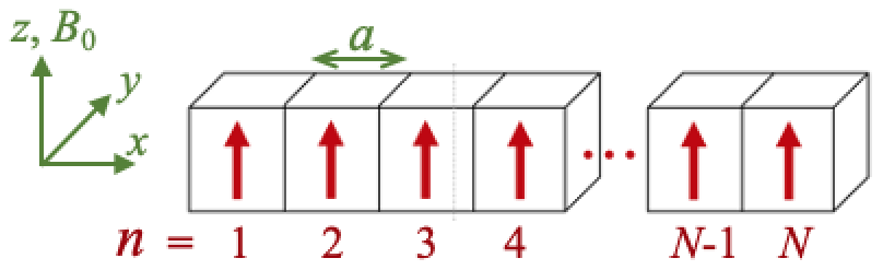
Figure 1: Geometry for a finite-length ferromagnetic chain with $N$ interacting spins along the $x$ axis with coordinates $x_{n}=na$ where $a$ is the separation between neighbouring spins and $n=1,2,3,\cdots,N$ is a spin label. In the absence of DMI the spins are aligned along the $z$ axis.

The Hamiltonian for the ferromagnetic chain can be written in terms of the spin operators $\mathbf{S}_{n}$ at site $n$ as

$$\mathcal{H} = -\frac{1}{2}\underset{n,m}{\sum}J_{n,m}\mathbf{S}_{n}\cdot\mathbf{S}_{m}-\frac{1}{2}\underset{n,m}{\sum}\boldsymbol{\mathit{J}}_{M\mathit{n,m}}\cdot(\mathbf{S}_{n}\times\mathbf{S}_{m})$$ (1)

$$+\frac{1}{2}\underset{n,m}{\sum}\underset{\alpha,\beta}{\sum}D_{n,m}^{\alpha\beta}S_{n}^{\alpha}S_{m}^{\beta}-g\mu_{B}B_{0}\underset{n}{\sum}S_{n}^{z}.$$

Here, the first two terms represent the bilinear exchange and the DMI, respectively, with the exchange parameters $J_{n,m}$ and $\boldsymbol{J}_{Mn,m}$ being symmetric and antisymmetric with respect to the spin labels $n$ and $m$. We note that $\boldsymbol{J}_{Mn,m}$ is an axial vector, which may in principle be directed along any of the $x$, $y$, or $z$ directions. The third term in the Hamiltonian is the contribution due to the long-range dipole-dipole interactions along the chain, where the interaction term is (with $\alpha$ and $\beta$ denoting Cartesian componemts $x$, $y$, or $z$):

$$D_{n,m}^{\alpha\beta} = (g\mu_{B})^{2}\frac{\left|\mathbf{r}_{n,m}\right|^{2}\delta_{\alpha\beta}-3r_{n,m}^{\alpha}r_{n,m}^{\beta}}{\left|\mathbf{r}_{n,m}\right|^{5}}.$$ (2)

Here $\mathbf{r}_{n,m}$ is the vector separation between sites $n$ and $m$, $g$ is the Landé factor, and $\mu_{B}$ denotes the Bohr magneton. In the chain geometry, the only nonzero dipole-dipole coefficients correspond to the diagonal terms $D_{n,m}^{yy}=D_{n,m}^{zz}=-\frac{1}{2}D_{n,m}^{xx}\equiv d_{n,m}$, where $d_{n,m}=(g\mu_{B})^{2}/(|n-m|a)^{3}$ for $n\neq m$ and is zero otherwise. The final term in Eq. (1) represents the Zeeman energy due to the applied magnetic field $B_{0}$ in the $z$ direction.

It will be assumed that the two types of exchange terms couple only nearest neighbours. Initially, we shall take these interactions to have the same (bulk) values between all sites, but in a later section end perturbations will be introduced to study spin-wave mode localization. Specifically, we take here $J_{n,m}=J\delta_{n\pm 1,m}$ and $J_{n,m}=\pm J_{M}\delta_{n\pm 1,m}$ for the symmetric and antisymmetric exchange terms, where $J>0$ for a ferromagnet but the weaker $J_{M}$ may have have either sign.

A calculation was recently given by Moon et al. Moon-2013 for an infinite chain of spins with nearest-neighbour Heisenberg exchange coupling and DMI. Here we are considering the behaviour of finite-length chains when DMI is present, along with an applied field, Heisenberg exchange, and dipole-dipole interactions. Thus, by contrast with Moon-2013 , there will be edge effects near the ends of the chain, which may cause the spins to tilt away from the $z$ axis (the field direction). We now explore the three different cases for the direction of the DMI axial vector.

II.1 DMI axis along $\boldsymbol{\hat{z}}$ direction

We write for this case $\boldsymbol{\mathit{J}}_{M\mathit{n,m}}=\boldsymbol{\hat{z}}J_{Mn,m}$, so the DMI term in the Hamiltonian involves the combination $\boldsymbol{\hat{z}}\cdot(\mathbf{S}_{n}\times\mathbf{S}_{m})=S_{n}^{x}S_{m}^{y}-S_{n}^{y}S_{m}^{x}.$ In order to find the equilibrium orientations of the spins along the chain, we proceed by writing down an energy functional $\bar{E}$, deduced from the total Hamiltonian terms in a mean field approximation.

$$\bar{E} = -\frac{1}{2}\underset{n,m}{\sum}[J_{n,m}\{S_{n}^{x}S_{m}^{x}+S_{n}^{y}S_{m}^{y}+S_{n}^{z}S_{m}^{z}\}+J_{Mn,n}(S_{n}^{x}S_{m}^{y}-S_{n}^{y}S_{m}^{x})$$ (3)

$$+(g\mu_{B})^{2}d_{n,m}\{2S_{n}^{x}S_{m}^{x}-S_{n}^{y}S_{m}^{y}-S_{n}^{z}S_{m}^{z}\}]-g\mu_{B}B_{0}\sum_{n}S_{n}^{z}.$$

Then, the components of the effective field $\mathbf{B}_{eff,n}$ acting on any spin $n$ are calculated from

$$B_{eff,n}^{\alpha} = -\frac{1}{g\mu_{B}}\,\frac{\delta E}{\delta S_{n}^{\alpha}}\quad(\alpha=x,y,z),$$ (4)

giving rise to a set of $3N$ coupled equations ($n=1,2,\cdots N$):

$$B_{eff,n}^{x} = \frac{1}{g\mu_{B}}\sum_{m}\{(J_{n,m}+d_{n,m})S_{m}^{x}+J_{Mn,m}S_{m}^{y}\},$$ (5)

$$B_{eff,n}^{y} = \frac{1}{g\mu_{B}}\sum_{m}\{(J_{n,m}-\frac{1}{2}d_{n,m})S_{m}^{y}-J_{Mn,m}S_{m}^{x}\},$$ (6)

$$B_{eff,n}^{z} = B_{0}+\frac{1}{g\mu_{B}}\sum_{m}(J_{n,m}S_{m}^{z}-\frac{1}{2}d_{n,m})S_{m}^{z}.$$ (7)

These equations take a simple form, where it is seen that the transverse ($x$ and $y$ components) of the effective fields do not couple to any longitudinal ($z$) component of a spin. This means that the equations can all be satisfied by taking $S_{n}^{x}=S_{n}^{y}=0$ (for all $n$), and hence $S_{n}^{z}=S$. In other words, there is no tilting effect for this particular choice of DMI axis (by contrast with the situation for the other two choices of DMI axis later). It is easily verified that the above solution is indeed the stable equilibrium solution, provided $B_{0}$ is sufficiently large to overcome the static demagnetizing effects in the $z$ direction.

Turning next to the spin-wave dynamics, we may follow steps analogous to those in Nguyen-2005b ; Lupo-2016 by transforming the spin Hamiltonian (1) to boson operators using the Holstein-Primakoff transformation Holstein-1940 relative to the local axes (which coincide with the global $x$, $y$ and $z$ axes in this case). The total Hamiltonian can be expanded as $\mathcal{H}=\mathcal{H}^{(0)}+\mathcal{H}^{(1)}+\mathcal{H}^{(2)}+\mathcal{H}^{(3)}+...$, where $\mathcal{H}^{(s)}$ denotes a term with $s$ boson operators, the first term is a constant and $\mathcal{H}^{(1)}$ vanishes by symmetry. Therefore, for the linearized SWs we are concerned only with the quadratic term, which can be written in a bilinear form as

$$\mathcal{H}^{(2)} = \underset{n,m}{\sum}\{A_{n,m}a_{n}^{\dagger}a_{m}+B_{n,m}(a_{n}^{\dagger}a_{m}^{\dagger}+a_{n}a_{m})\},$$ (8)

where $A_{n,m}$ and $B_{n,m}$ may be regarded as elements of $N\times N$ matrices $\boldsymbol{A}$ and $\boldsymbol{B}$ with

$$A_{n,m} = A_{n}^{0}\delta_{n,m}-SJ_{n,m}+iSJ_{Mn,m}-\frac{1}{2}Sd_{n,m},$$ (9)

$$A_{n}^{0} = B_{n,m}g\mu_{B}B_{0}+S\sum_{p=1}^{N}\{J_{n,p}-d_{n,p}\},\quad B_{n,m}=-\frac{3}{4}Sd_{n,m}.$$ (10)

The final step in determining the SW frequencies and their amplitudes is to diagonalize $\mathcal{H}^{(2)}$ using a generalized Bogoliubov transformation (described in Nguyen-2005b ; Lupo-2016 ). This eventually gives rise to a dynamical block matrix defined by

$$\left(\begin{array}[]{cc}\boldsymbol{A}^{(2)}&2\boldsymbol{B}^{(2)}\\ -2\boldsymbol{B}^{(2)*}&-\tilde{\boldsymbol{A}}^{(2)}\end{array}\right),$$ (11)

where the tilde denotes a matrix transpose. The positive eigenvalues of the above large matrix correspond to the total of $N$ physical SW frequencies; there is a set of degenerate (in magnitude) frequencies formed by the negative eigenvalues. The “diagonalized” form of $\mathcal{H}^{(2)}$ can be expressed as

$$\mathcal{H}^{(2)}=\sum_{l=1}^{N}\omega_{l}\,b_{l}^{\dagger}b_{l},$$ (12)

where $\omega_{l}$ are the discrete spin-wave modes with integer $l=1,\,2,\,\ldots\,,N$ being a branch number, while $b_{l}^{\dagger}$ and $b_{l}$ are the transformed (diagonalized) boson operators for creation and annihilation of mode $l$. The eigenvectors of the matrix in Eq. (11) provide us with the spatially-dependent complex amplitudes Hussain-2022 , i.e. with the relative phase information included. Numerical examples of the application of the above results will be given in Sec. III.

II.2 DMI axis along $\boldsymbol{\hat{x}}$ direction

We next turn to the more interesting situation when the direction of the DMI axis lies along the chain length $x$. The DMI term of spin Hamiltonian now involves the combination $\boldsymbol{\hat{x}}\cdot(\mathbf{S}_{n}\times\mathbf{S}_{m})=S_{n}^{y}S_{m}^{z}-S_{n}^{z}S_{m}^{y}$. We may follow the analogous steps as in Sec. IIB in forming an energy functional and the effective field components on any spin. The modified equations are

$$B_{eff,n}^{x} = \frac{1}{g\mu_{B}}\sum_{m}(J_{n,m}+d_{n,m})S_{m}^{x},$$ (13)

$$B_{eff,n}^{y} = \frac{1}{g\mu_{B}}\{\sum_{m}\{(J_{n,m}-\frac{1}{2}d_{n,m})S_{m}^{y}+J_{Mn,m}S_{m}^{z}\},$$ (14)

$$B_{eff,n}^{z} = B_{0}+\frac{1}{g\mu_{B}}\sum_{m}\{(J_{n,m}-\frac{1}{2}d_{n,m})S_{m}^{z}-J_{Mn,m}S_{m}^{y}\}.$$ (15)

It is seen from the above that there is a coupling between the $S^{y}$ and $S^{z}$ spin components along the chain, but the expression for the $B_{eff}^{x}$ field involves only $S^{x}$. A careful analysis (also confirmed in the numerical calculation) shows that the spins along the chain are tilted in the $yz$ plane away from the $z$ direction through an angle $\theta_{n}$ for spin $n$. The effect is more pronounced near the end of the chain; it is a consequence of the antisymmetry of the DMI terms and missing exchange interactions at the ends.

To solve for the tilt angles, we may re-express the mean-field spin components on the right-hand side of Eqs. (13)-(15) using $\mathbf{S}_{n}=S(0,\sin\theta_{n},\cos\theta_{n})$, giving

$$\textnormal{sin}\theta_{n} = \frac{B_{eff,n}^{y}}{\sqrt{(B_{eff,n}^{y})^{2}+(B_{eff,n}^{z})^{2}}},\quad\cos\theta_{n}=\frac{B_{eff,n}^{z}}{\sqrt{(B_{eff,n}^{y})^{2}+(B_{eff,n}^{z})^{2}}}.$$ (16)

The equilibrium orientations may then be deduced numerically solution from Eqs. (14)-(16) through an iterative process (e.g., by analogy with Lupo-2016 ; Hussain-2022 ). Briefly, an initial configuration of the angles is chosen to approximate the ground state. In practice, we need to employ several starting configurations in order to avoid difficulties with local minima and to find the true ground state at $T\approx 0$. For example, a configuration to approximate spin alignment along the $z$ direction could be chosen. Next, each spin can be rotated to be along the direction of its local effective field, giving a new set of angles. This process can be repeated iteratively until convergence to a self-consistent static-equilibrium configuration is achieved, giving the required set of angles. As part of this process, it is neccessary to check which of the configurations leads to the lowest (global) minimum energy. When the stable spin configuration has been determined, we may use the set of final angles to transform from the global coordinates ($x,y,z$) to a set of local coordinates ($X,Y,Z$) chosen such that the new $Z$ axis is along the equilibrium direction of each spin.

Then we determine the spin-wave properties following analogous steps to those described in the previous subsection. An important difference is that the Holstein-Primakoff transformation to boson operators is introduced relative to the local spin coordinates. It is found that Eqs. (8), (11) and (12) are still formally applicable, except that the matrix elements are now given by

$$A_{n,m} = A_{n}^{0}\delta_{n,m}-\frac{1}{2}S\{J_{n,m}[1+\cos(\theta_{n}-\theta_{m})]+J_{Mn,m}\sin(\theta_{n}-\theta_{m})$$ (17)

$$+d_{n,m}[2-\cos(\theta_{n}-\theta_{m})]\},$$

$$A_{n}^{0} = g\mu_{B}B_{0}\cos\theta_{n}+S\sum_{p}\{J_{n,p}\cos(\theta_{n}-\theta_{p})+J_{Mn,p}\sin(\theta_{n}-\theta_{p})$$ (18)

$$-d_{n,p}\cos(\theta_{n}-\theta_{p})\},$$

$$B_{n,m} = -\frac{1}{4}S\{J_{n,m}[1-\cos(\theta_{n}-\theta_{m})]-J_{Mn,m}\sin(\theta_{n}-\theta_{m})$$ (19)

$$+d_{n,m}[2+\cos(\theta_{n}-\theta_{m})]\}.$$

II.3 DMI axis along $\boldsymbol{\hat{y}}$ direction

The final case to consider is when the DMI axial vector is along the $y$ direction, for which $\boldsymbol{\hat{y}}\cdot(\mathbf{S}_{n}\times\mathbf{S}_{m})=S_{n}^{z}S_{m}^{x}-S_{n}^{x}S_{m}^{z}$. It is straightforward to show that the coupled equations for the components of the effective mean fields become

$$B_{eff,n}^{x} = \frac{1}{g\mu_{B}}\{\sum_{m}(J_{n,m}+d_{n,m})S_{m}^{x}-\sum_{m}J_{Mn,m}S_{m}^{z}\},$$ (20)

$$B_{eff,n}^{y} = \frac{1}{g\mu_{B}}\sum_{m}(J_{n,m}-\frac{1}{2}d_{n,m})S_{m}^{y},$$ (21)

$$B_{eff,n}^{z} = B_{0}+\frac{1}{g\mu_{B}}\{\sum_{m}(J_{n,m}-\frac{1}{2}d_{n,m})S_{m}^{z}+J_{Mn,m}S_{m}^{x}\}.$$ (22)

Here it is seen that that there is a coupling between the $S^{x}$ and $S^{z}$ spin components along the chain, while the expression for the $B_{eff}^{y}$ field involves only $S^{y}$. By analogy with the previous subsection, if follows that the spins along the chain are now tilted in the $xz$ plane away from the $z$ direction through an angle denoted as $\phi_{n}$. Instead of Eq. (16), we now have $\mathbf{S}_{n}=S(\sin\phi_{n},0,\cos\phi_{n})$, with

$$\textnormal{sin}\phi_{n} = \frac{B_{eff,n}^{x}}{\sqrt{(B_{eff,n}^{x})^{2}+(B_{eff,n}^{z})^{2}}},\quad\cos\phi_{n}=\frac{B_{eff,n}^{z}}{\sqrt{(B_{eff,n}^{x})^{2}+(B_{eff,n}^{z})^{2}}}.$$ (23)

In a numerical application the equilibrium tilt angles may be found through an iterative process, as described earlier.

The calculations for the spin-wave excitations then proceeds in an analogous fashion to the previous subsection. The coefficients of the quadratic Hamiltonian involve the tilt angles $\phi_{n}$ and have the modified form

$$A_{n,m} = A_{n}^{0}\delta_{n,m}-\frac{1}{2}S\{J_{n,m}[1+\cos(\phi_{n}-\phi_{m})]-J_{Mn,m}\sin(\phi_{n}-\phi_{m})$$ (24)

$$+d_{n,m}[(2\cos\theta_{n}\cos\theta_{m}-\sin\theta_{n}\sin\theta_{m}-1)\},$$

$$A_{n}^{0} = g\mu_{B}B_{0}\cos\phi_{n}+S\sum_{p}\{J_{n,p}\cos(\phi_{n}-\phi_{p})-J_{Mn,p}\sin(\phi_{n}-\phi_{p})$$ (25)

$$+d_{n,p}(2\sin\phi_{n}\sin\phi_{p}-\cos\phi_{n}\cos\phi_{p})\},$$

$$B_{n,m} = \frac{1}{4}S\{J_{n,m}[1-\cos(\phi_{n}-\phi_{m})]+J_{Mn,m}\sin(\phi_{n}-\phi_{m})$$ (26)

$$-d_{n,m}(2\cos\phi_{n}\cos\phi_{m}+\sin\phi_{n}\sin\phi_{m}+1)\}.$$

III Numerical results

In this section we present some numerical applications for the quantized spin-wave modes of finite chains, using the formal results for the three directions of DMI axial vector obtained in Sec. II. Examples will be given for several chain lengths ($N=15,$ 25, and 60), for DMI values ranging from $J_{M}/J=0$ up to 0.35, and for dipole-dipole strengths (relative to the bilinear exchange) such that $d=(g\mu_{B})^{2}/Ja{}^{3}=0$, 0.01, and 0.02. For convenience, we choose spin quantum number $S=1$ and an applied magnetic field such that $g\mu_{B}B_{0}/J=0.25.$

First, in Fig. 2 a plot is given of the spin-wave energy $E$ (in dimensionless units $E/SJ$) versus the DMI strength $J_{M}/J$ for a relatively short chain with $N=15$ and a fixed value $d=$ 0.02 of the dipolar strength. In this case (which is for the DMI along $z$) the variation with DMI strength on the individual modes is evident, giving a downwards shift for the lower modes and an upwards shift for the higher modes. This difference of behaviour is attributable to the fact that the amplitude oscillations for the lower modes are all in phase, whereas those for the higher modes are 180° out of phase for any site with respect to its nearest neighbours (see later for discussion of the amplitudes). All the spin-wave modes in this example are bulk modes with an oscillatory amplitude profile; the upper and upper boundaries of the bulk mode quasi-continuum are indicated by the black dashed lines in Fig. 2.

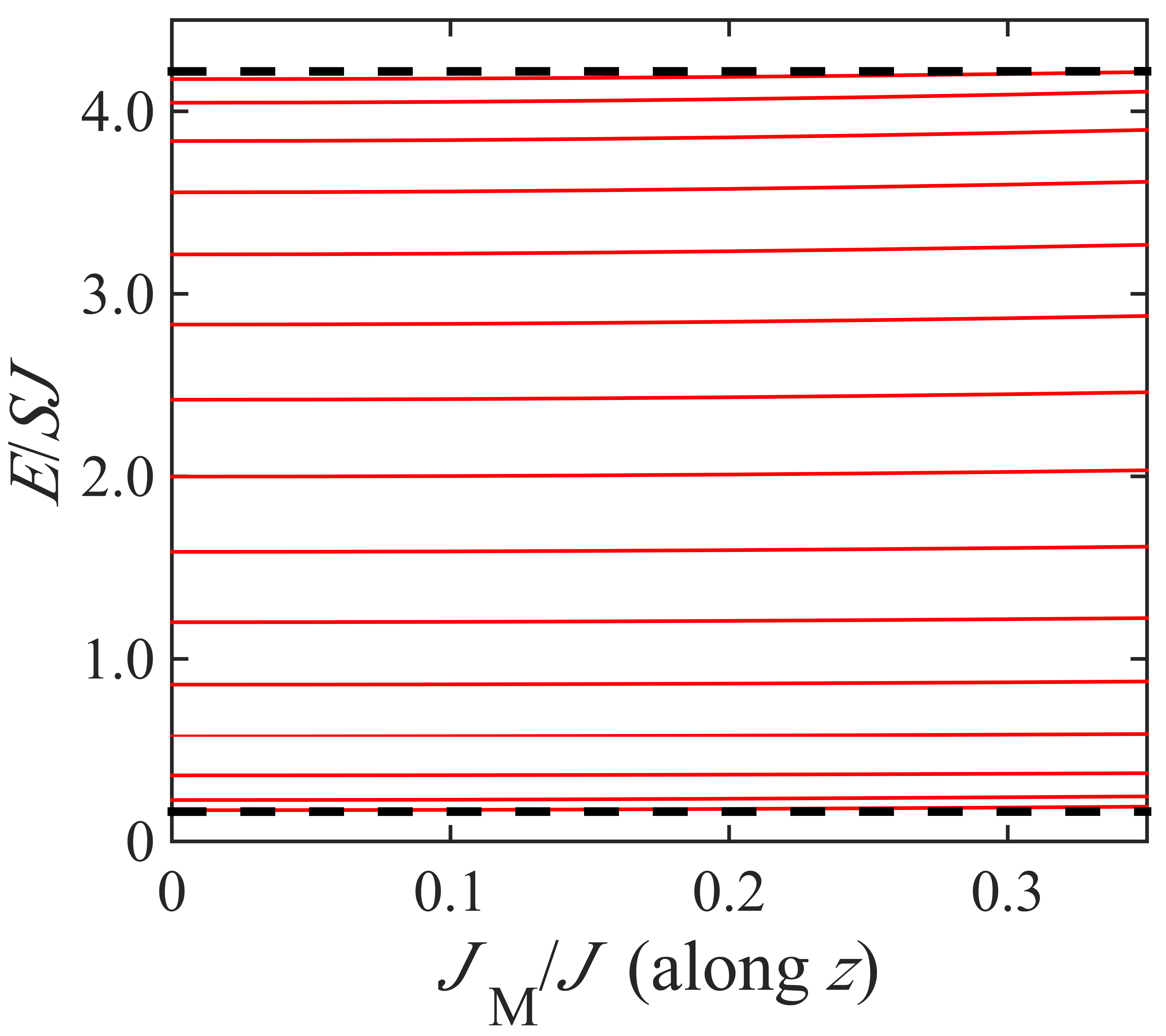
Figure 2: Plot of the spin-wave energy $E$ (in terms of the dimensionless $E/SJ$) versus relative DMI strength $J_{M}/J$ for a fixed $N=15$ showing all 15 branches (solid red lines). The DMI axis has been taken along the $z$ direction. The black dashed lines indicate the upper and lower boundaries of the bulk-mode region. See the text for other parameter values.

Next, in Fig. 3 we show some comparisons for the bulk-mode energies when the DMI axis is along the different principal directions ($x$, $y$ or $z$). Here the plots versus $J_{M}/J$ are shown for just the lowest three branches for longer chain lengths corresponding to (a) $N=25$ and (b) $N=60$. It is seen that, while the curves for the DMI along $z$ shift downwards with increasing $J_{M}/J$, as mentioned earlier, the curves for for the DMI along $x$ and $y$ shift slightly upwards. This difference in behaviour is presumed to be related to tilting of the end spins in the $x$ and $y$ cases. We illustrate in Fig. 4 some calculated values for the tilt angle $\theta_{n}$ for different spin site number $n$ when $N=25$ (as in Fig. 3a) and $J_{M}/J=0.2$. It can be seen that $\theta_{n}$ is largest in magnitude at the ends of the chain and the mode profile is antisymmetric with respect to the ends.

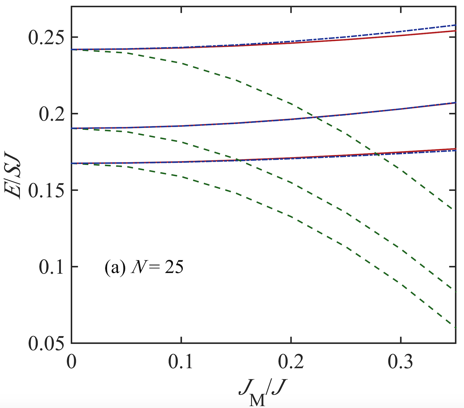
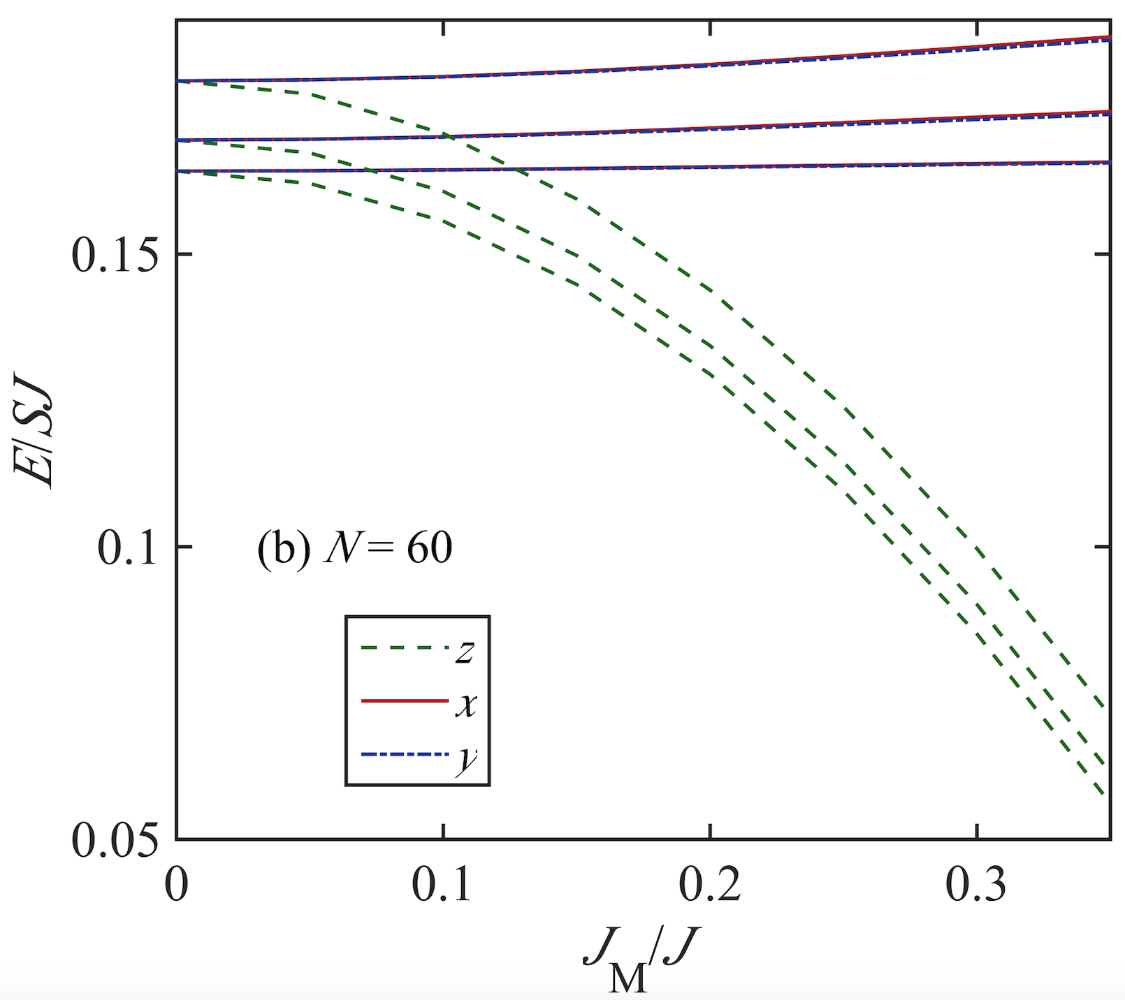
Figure 3: Plot of the spin-wave energy $E$ (in terms of the dimensionless $E/SJ$) versus relative DMI strength $J_{M}/J$ for (a) $N=25$ and (b) $N=60$ showing only the lowest three branches in each case. The three different types of lines (see the inset) correspond the the DMI axis along $x$, $y$, and $z$. See the text foe other parameter values.

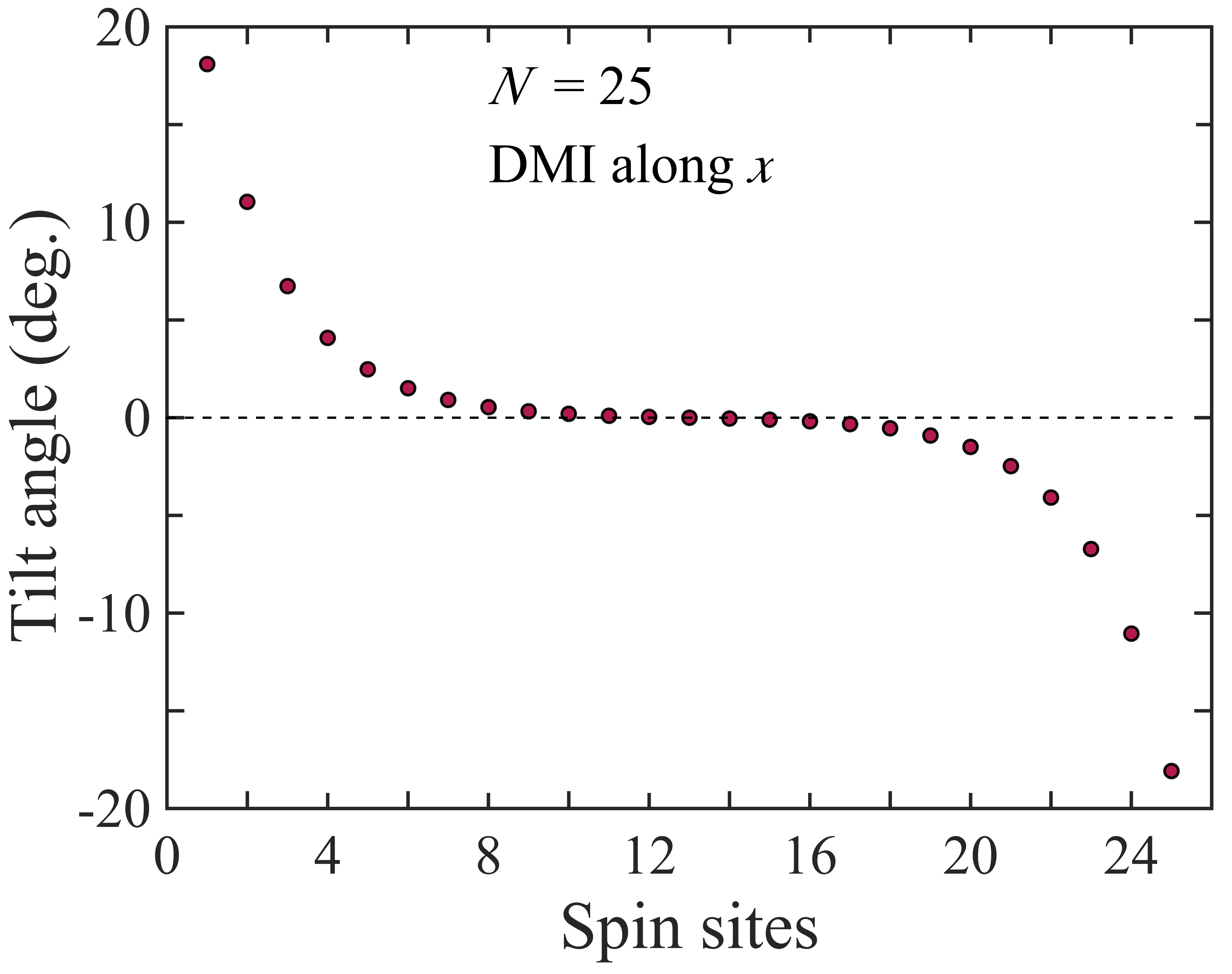
Figure 4: Plot of the tilt angles $\theta_{n}$ (in degrees) versus the spin number $n$ ($=1,2,\cdots,N$) choosing a chain with $N=25$ as in Fig. 3a and $J_{M}/J=0.2$.

In Fig. 5 we illustrate the role of the dipole-dipole interactions on the spin waves in this chain geometry. The plots in each case, which correspond to the DMI axis along $x$, are shown for dipole strength $d=0.0$ and 0.02, as indicated. The results are for just the lowest three modes in a chain with $N=25$. Note that $E$ for each spin-wave mode decreases, as expected, when the strength $d$ is increased.

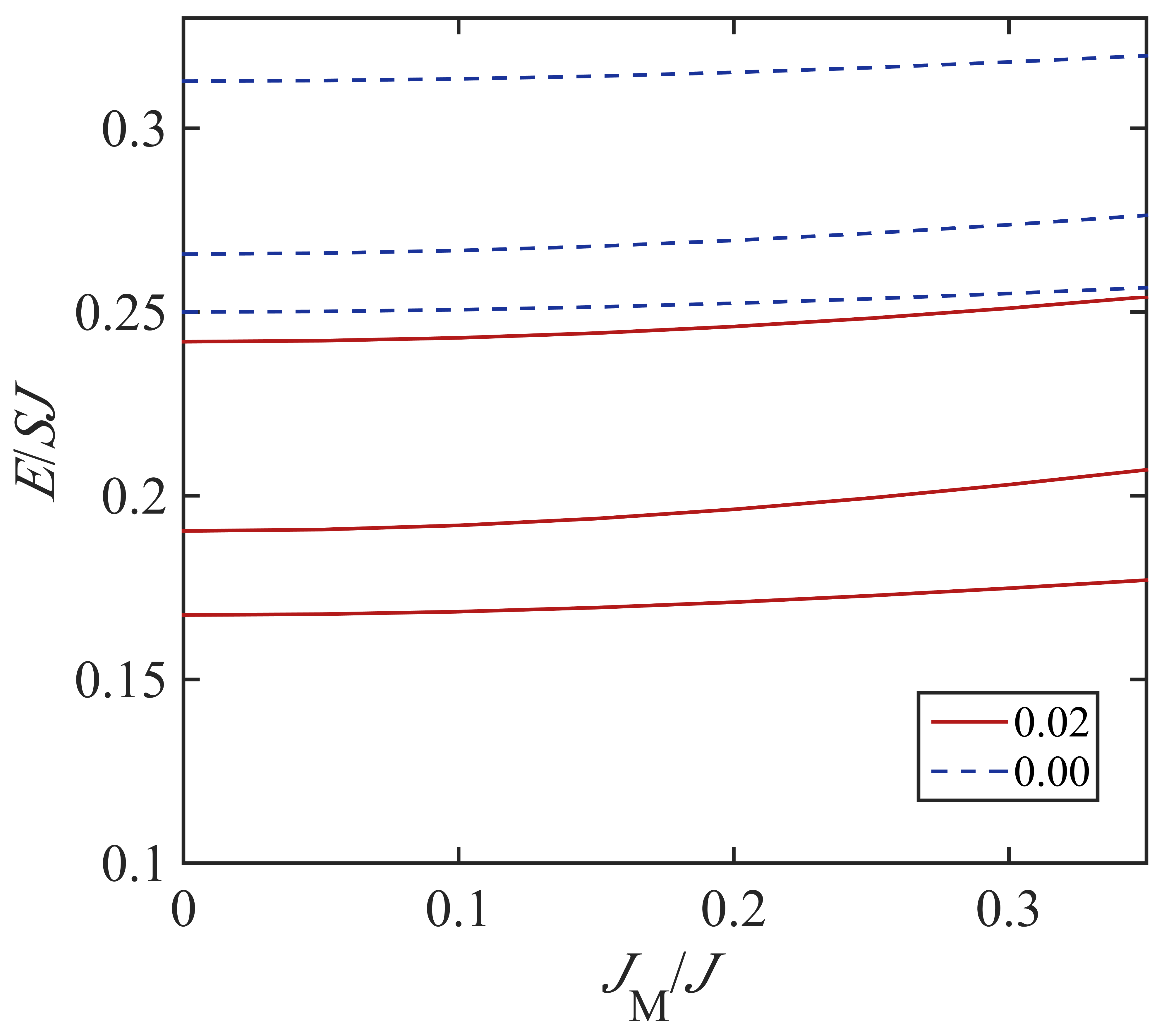
Figure 5: Plot of the spin-wave energy $E$ (in terms of the dimensionless $E/SJ$) versus relative DMI strength $J_{M}/J$, showing curves for three different dipole-dipole strengths $d=0.00$, 0.01, and 0.02. We depict only the three lowest spin-wave modes for a chain with $N=25$ for the case of DMI axis along $x$.

To conclude this section we present in Fig. 6 some plots of the spin-wave amplitude (with the relative phase included) versus the site number $n$ for the spins along the chain. We employ the eigenvector formalism described in Sec. II. In panel (a) we show the profiles for the lowest three modes. Mode 1 is the analogue of the uniform mode (but it shows some variation due to end effects), while modes 2 and 3 are wave-like in character. For the higher energy modes, like for mode 24 shown in panel (b), the complex amplitudes change sign (have a 180° change of phase) in going from any one site to its neighbour. This was mentioned earlier for the interpretation of Fig. 2.

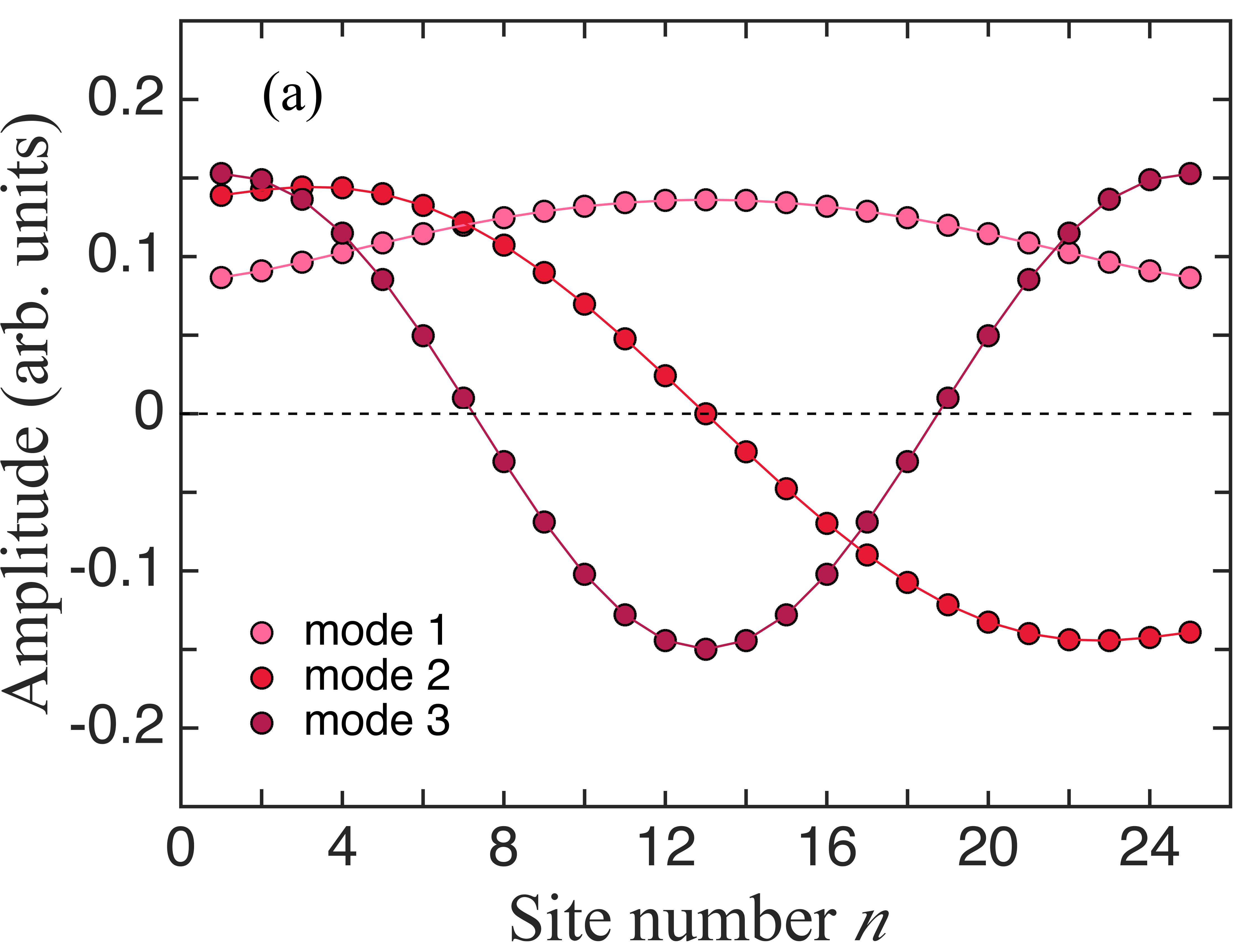
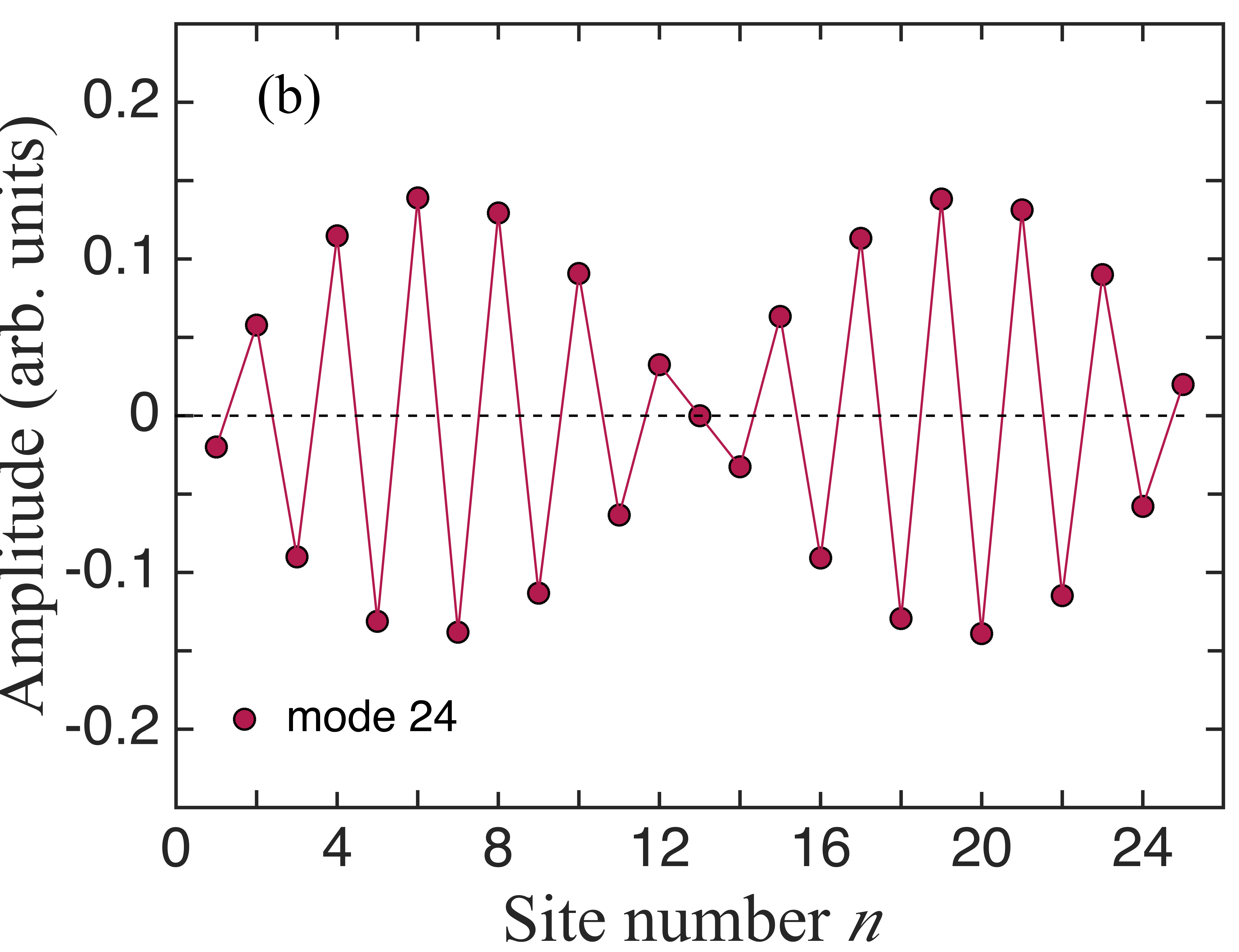
Figure 6: Plots to show the spin-wave amplitudes (in arbitrary units) versus the spin number $n$ ($=1,2,\cdots,N$) choosing a chain with $N=25$. The modes 1-3 are colour-coded as indicated in the inset to (a) and mode 24 is shown in (b). The DMI strength is $J_{M}/J$ = 0.2 along $x$ and the dipole-dipole strength is $d$ = 0.02. See the text for other parameters.

IV Mode localization effects

Up to now, all the spin-wave modes have had bulk-like propagation properties. We now examine the possibility of modifications to the end parameters of the chain in order to study possibilities for the occurrence of localized spin-wave modes. As a simple assumption, we will take the dominant nearest-neighbour symmetric bilinear exchange $J_{n,m}$ to be different at both ends of the chain. Therefore, we assume $J_{1,2}=J_{2,1}=J_{N-1,N}=J_{N,N-1}\equiv J_{S}$, whereas for all other nearest neighbours it is equal to the bulk value $J.$ The value of $J_{S}$ will typically depend on overlap integrals between wave functions at the pair of sites, and so may be modified compared with spins in the middle of the chain. In principle, $J_{S}$ can be either greater than or less than $J$.

The above property for $J_{S}$ can straightforwardly be accommodated into the theory given in Sec. II. In fact, all the formal expressions derived there still apply provided $J_{S}>0$. It is necessary only to use the generalized assumption for $J_{n,m}$ in the numerical calculations for the equilibrium tilt angles and for finding the eigenvalues and eigenvectors of the dynaical matrix in Eq. (11).

It is interesting to note that there is a special case in which the solution for the dynamical matrix can be carried out analytically. This occurs in the case of the DMI axial vector along $z$ (so the tilt angles are zero) when the dipole-dipole interactions are absent ($d=0$) and the chain is semi-infinite ($N\rightarrow\infty$). Then matrix $\boldsymbol{B}$ vanishes and matrix $\boldsymbol{A}$ simplifies, leaving the dynamical matrix expressible in a tridiagonal form as

$$SJ\left(\begin{array}[]{cccccc}c_{0}&-\gamma+i\alpha&0&0&0&\cdots\\ -\gamma-i\alpha&c^{\prime}&-1+i\alpha&0&0&\cdots\\ 0&-1-i\alpha&c&-1+i\alpha&0&\cdots\\ 0&0&-1-i\alpha&c&-1+i\alpha&\cdots\\ 0&0&0&-1-i\alpha&c&\cdots\\ \vdots&\vdots&\vdots&\vdots&\vdots&\ddots\end{array}\right),$$ (27)

where we define the ratios $\gamma=J_{S}/J$ and $\alpha=J_{M}/J$, while $c_{0}=\gamma+(g\mu_{B}B_{0}/SJ)$, $c^{\prime}=1+\gamma+(g\mu_{B}B_{0}/SJ)$, and $c=2+(g\mu_{B}B_{0}/SJ)$. It follows that the perturbing effects of the end of the chain are confined to the top left $2\times 2$ block of this matrix, while elsewhere the matrix elements are constant along the main diagonal and the diagonal lines above and below. This is of significance here, because it is well known that the determinant of tridiagonal matrices with these properties can be found analytically (see, e.g., Dewames-1969 ; Wolfram-1972 ; Cottam-1976 for semi-infinite Heisenberg ferromagnets). Hence the eigenvaluesof the dynamical matrix, which are just the spin-wave energies, can be deduced. The result from following an analogous approach here is that a localized surface spin wave can exist only when $J_{S}/J$ exceeds a threshold value of 4/3, or approximately 1.33, in which case the surface-mode energy lies above the top of the bulk region. The derivation is outlined in the Appendix.

We now present some numerical results obtained, as described earlier, for the general case, i.e, with dipole-dipole interactions included and with $N$ taking a finite value. In Fig. 7 a plot is shown for the spin-wave energies versus $J_{M}/J$ for the DMI axial vector along $z$ when $J_{S}/J$ = 1.8 and $N$ = 15. It is seen that there are thirteen modes within the bulk-mode region (between the black dashed lines) and two almost-degenerate modes labelled S above the top of the bulk region. The latter are the surface modes (one at each end of the chain). This plot may be compared with Fig. 2 for $J_{S}/J$ = 1.0, where all fifteen of the spin-wave modes are bulk-like.

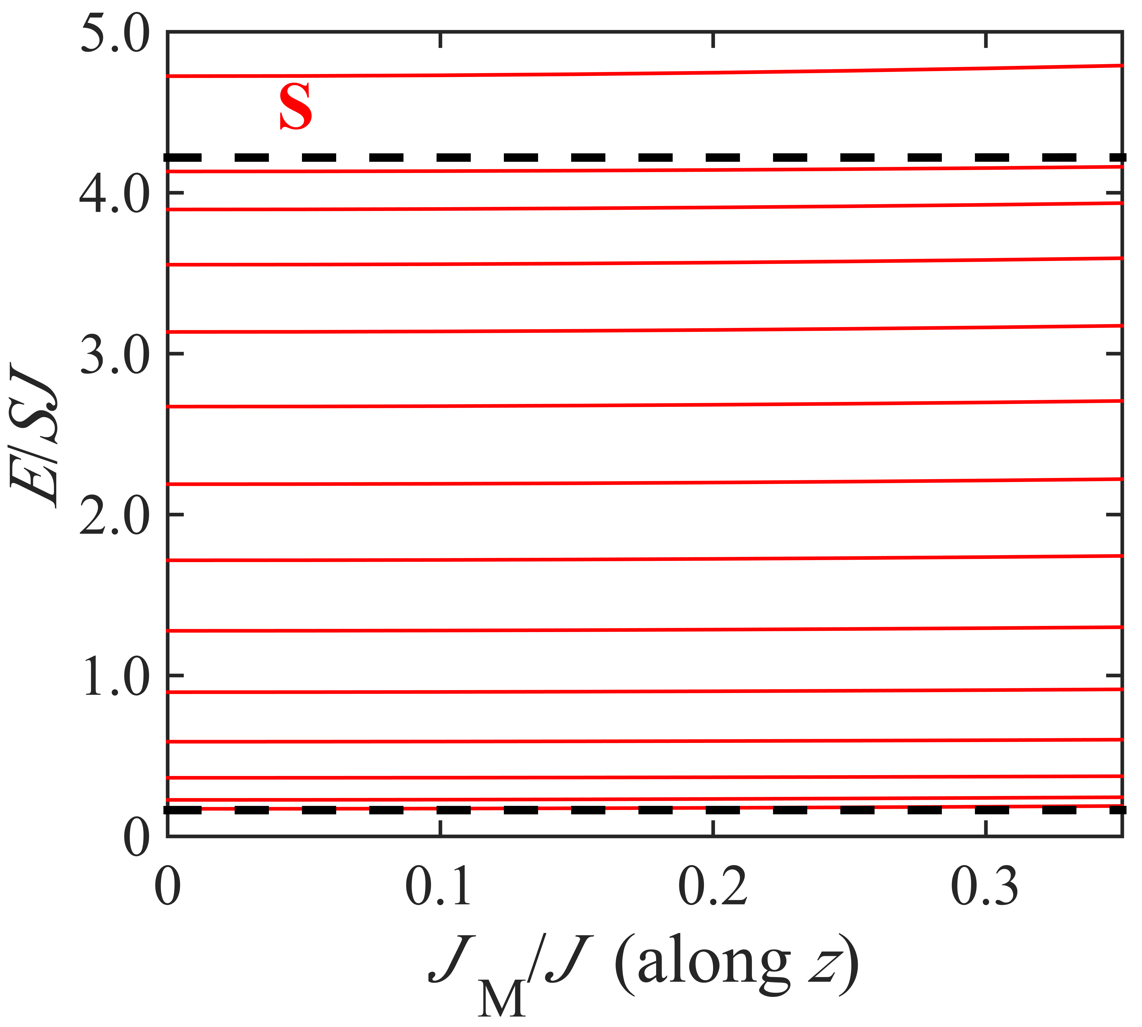
Figure 7: Plot of the spin-wave energy $E$ (in terms of the dimensionless $E/SJ$) versus relative DMI strength $J_{M}/J$ for fixed $N=15$ showing all the spin-wave branches when $J_{S}/J=1.8$ taking the DMI axial vector along $z$. The black dashed lines indicate the upper and lower boundaries of the bulk-mode region. Other parameters are as in Fig. 2.

In Fig. 8 we show the several surface spin energies for different choices of $J_{S}/J$ (as labelled) when plotted versus $J_{M}/J$. Here $N$ = 60 and the DMI axial vector is along $x$. The surface modes are found occur at higher energies as $J_{S}/J$ is increased, starting here at 1.4 which is just above the threshold value estimated earlier.

Figure 8: Plot of spin-wave energy $E$ (in terms of the dimensionless $E/SJ$) versus relative DMI strength $J_{M}/J$ for fixed $N=60$ showing only the surface spin-wave branches for several values of $J_{S}/J$ (= 1.4, 1.6, 1.8 and 2), as labelled. Here the DMI axial vector is along the $x$ axis. The black dashed line indicate the upper boundary of the bulk-mode region.

Finally, in Fig. 9 we show amplitude plots for the surface spin waves at two different values of $J_{S}/J$ (1.4 in panel a and 1.6 in panel b) versus the spin number $n$ choosing a chain with $N=25$. Modes 24 and 25 are shown, representing the two almost degenerate surface spin waves. It is seen that the amplitude profiles have decay characteristics away from the ends of the chain, by contrast with the behaviour in Fig. 6(b) when $J_{S}/J$ = 1.0. Also, the spatial decay is more rapid in Fig. 9 for the modes with the higher value of $J_{S}/J$ which correspond to the higher energy.

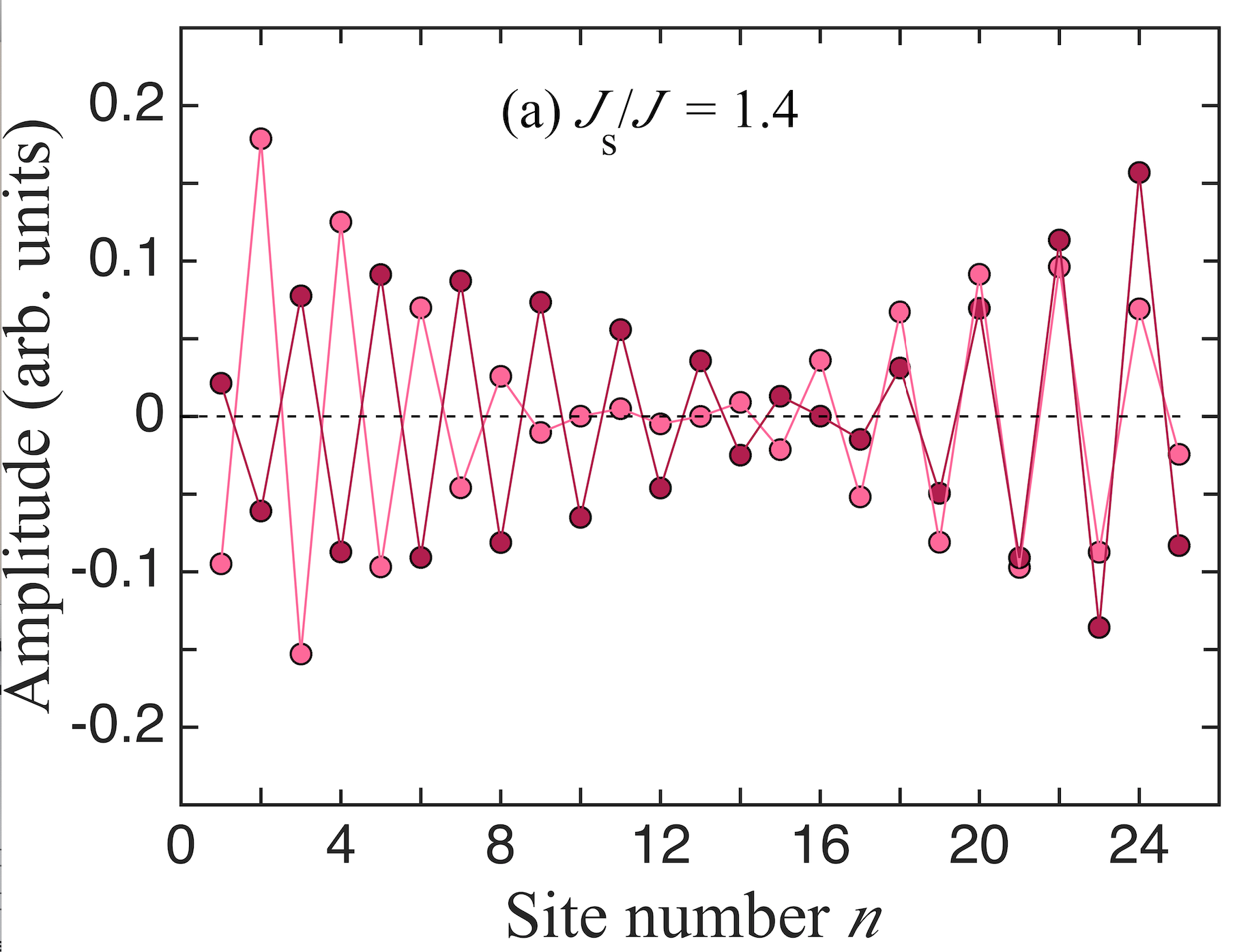
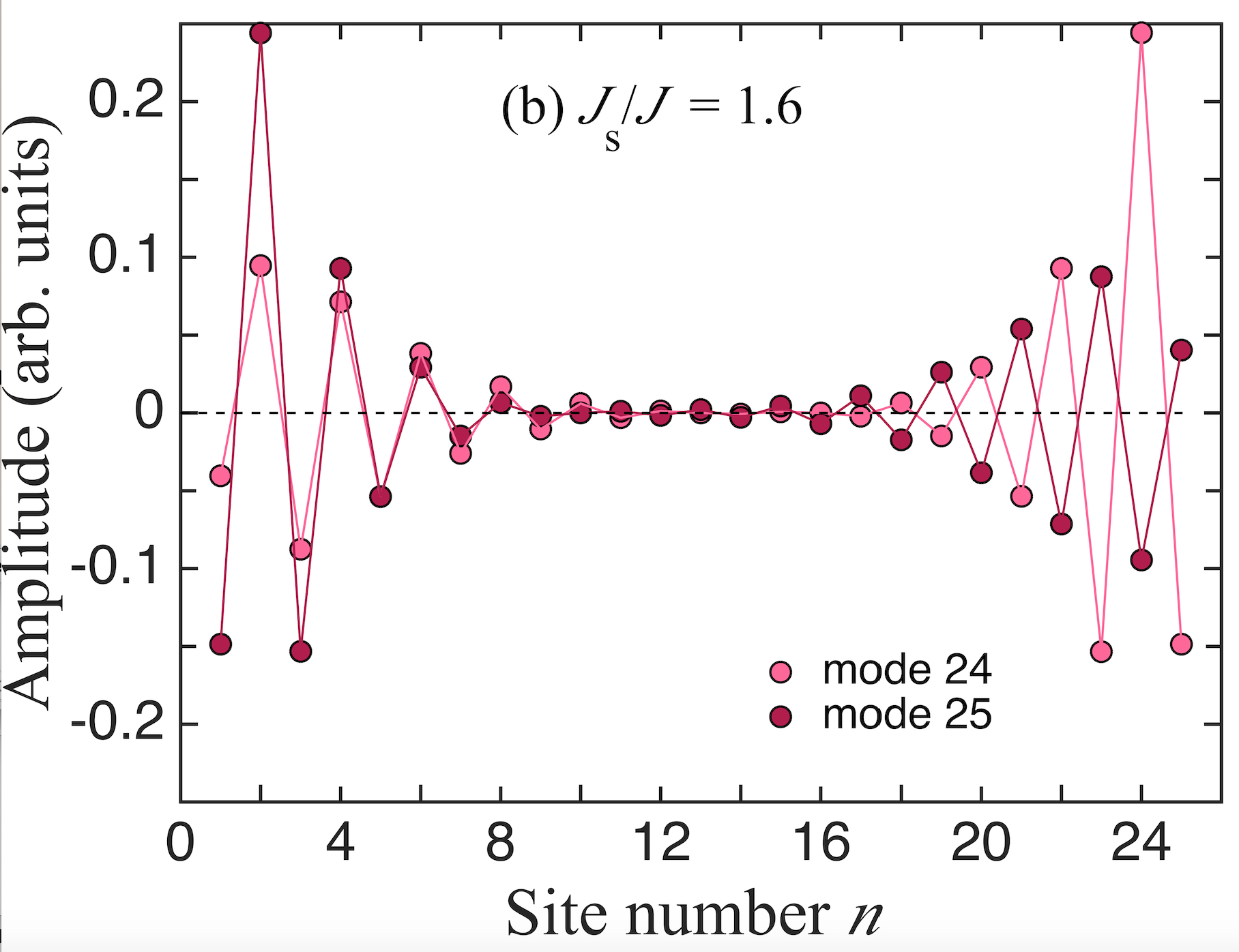
Figure 9: Plots to show the surface spin-wave amplitudes (in arbitrary units) when $J_{S}/J\neq 1$ versus the spin number $n$ ($1,2,\cdots,N$) choosing a chain with $N=25$. The data are shown for (a) $J_{S}/J=$ 1.4 and (b) $J_{S}/J=$ 1.6. We have taken $d=$ 0.02, $J_{M}/J=$ 0.2, and the DMI axial vector along $z$.

V Conclusions

In this paper we have presented theoretical studies for the magnetization dynamics for finite-length spin chains in the presence of DMI. We included bilinear exchange interactions and the long-range dipole-dipole interactions within a microscopic Hamiltonian operator formalism to investigate how the dipole-exchange spin waves are influenced by the DMI. We found that, when the DMI is included, three physically distinct situations arise depending on whether the direction of the axial vector associated with the DMI is chosen to be parallel to the chain length (along the $x$ axis) or in one of the perpendicular directions ($y$ or $z$ axis). All three cases were analyzed, and it was found that the static spin orientations and the dynamics (the mode localization and frequencies of the spin waves) are significantly modified by the DMI due to the competing interactions, which include the long-range dipole-dipole interactions. In some cases, the termination conditions occurring at the two ends of the chain lead to the prediction of localized spin waves (occurring above the bulk band) that have decay characteristics along the chain.

Although the DMI calculations presented here have been presented in terms of a finite linear-chain geometry, they are of wider applicability. For example, with only minor modifications to allow for additional contributions to the static dipolar fields, the results obtained here can be applied to finite-width nanowire stripes when the spin waves are excited with zero wave vector along the nanowire length. This work also provides a stepping stone to further DMI studies in which generalizations are made to other nanostructures, such as nanorings with different directions chosen for the DMI axial vector.

Appendix

Here we outline the steps involved in deducing the mode localization condition and mode energy from the tridiagonal matrix in Eq. (25). It is seen that the $2\times 2$ matrix $\boldsymbol{\Delta}$ representing the perturbation has the matrix elements $\Delta_{1,1}=c_{0}-c=\gamma-2$, $\Delta_{2,2}=c^{\prime}-c=\gamma-1$, and $\Delta_{1,2}=\Delta_{2,1}=-\gamma+1$. We may then employ the general result expressed in Eq. (60) of Cottam-1976 that any localized surface spin wave (having decaying amplitude away from the surface of the semi-infinite structure) has energy $E_{S}$ where

$$E_{S}=c-(x+x^{-1}),$$ (28)

where $|x|<1$ as a localization condition and the factor $x$ satisfies the cubic equation

$$h(x) \equiv 1+x(\Delta_{1,1}+\Delta_{2,2})+x^{2}(2\Delta_{1,2}+\Delta_{1,1}\Delta_{2,2}-\Delta_{1,2}^{2})+x^{3}\Delta_{2,2}$$ (29)

$$= 1+x(2\gamma-3)-3x^{2}(\gamma-1)+x^{3}(\gamma-1)=0.$$

A careful analysis shows that a physical solution for $x$ exists only if $\gamma>4/3$, which is the condition stated in Sec. IV. The mode energy, which is obtained using Eq. (28), then satisfies $E_{S}>c+2,$ which means that it occurs above the top of the bulk band.

- [1] I. Ye. Dzyaloshinskii. Sov. Phys. JETP, 5:1259, 1957.
- [2] T. Moriya. Phys. Rev., 120:91, 1960.
- [3] R. L. Melcher. Phys. Rev. Lett., 30:125, 1973.
- [4] J.-H. Moon, S.-M. Seo, K.-J. Lee, K.-W. Kim, J. Ryu, H.-W. Lee, R. D. McMichael, and M. D. Stiles. Phys. Rev. B, 88:184404, 2013.
- [5] K. Zakeri, Y. Zhang, J. Prokop, T.-H. Chuang, N. Sakr, W. X. Tang, and J. Kirschner. Phys. Rev. Lett., 104:137203, 2010.
- [6] D. Cortés-Ortuno and P. Landeros. J. Phys: Condens. Matter, 25:156001, 2013.
- [7] M. Kostylev. J. Appl. Phys., 115:233902, 2014.
- [8] A. K. Chaurasiya, C. Banerjee, S. Pan, S. Sahoo, S. Choudhury, J. Sinha, and A. Barman. Sci. Reps., 6:32592, 2016.
- [9] S. Tacchi, R. E. Troncoso, M. Ahlberg, G. Gubbiotti, M. Madami, J. Akerman, and P. Landeros. Phys. Rev. Lett., 118:147201, 2017.
- [10] H. Bouloussa, Y. Roussigné, M. Belmeguenai, A. Stashkevich, S.-M. Chérif, S. D. Pollard, and H. Yang. Phys. Rev. B, 102:014412, 2020.
- [11] R. Silvani, M. Alumni, S. Tacchi, and G. Carlotti. Appl. Sci., 11:2929, 2021.
- [12] J. Chen, H. Yu, and G. Gubbiotti. J. Phys. D: Appl. Phys., 55:123001, 2022.
- [13] R. A. Gallardo, D. Corteś-Ortuno, R. E. Troncoso, and P. Landeros. In G. Gubbiotti, editor, Three-Dimensional Magnonics, page 121. Jenny Stanford, 2019.
- [14] K. Zakeri. J. Phys.: Condens. Matter, 32:363001, 2020.
- [15] R. Gallardo, P. Alvarado-Seguel, and P. Landeros. Physical Review Applied, 18, 2022.
- [16] M. Shen, X. Li, Y. Zhang, X. Yang, and S. Chen. J. Phys. D: Appl. Phys., 55:213002, 2022.
- [17] S. Komineas and N. Papanicolaou. Phys. Rev B., 92:064412, 2015.
- [18] A. Barman et al. J. Phys.: Condens. Mater., 33:413001, 2021.
- [19] C. Q. Flores, C. Chalifour, J. Davidson, K. L. Livesey, and K. S. Buchanan. Phys. Rev. B, 102:024439, 2020.
- [20] B. Hussain and M. G. Cottam. J. Appl. Phys., 132:193901, 2022.
- [21] J. Villain. J. Phys. Chem. Solids, 11:303, 1959.
- [22] Y. Kim. Phys. Rev. B, 90:060401(R), 2014.
- [23] T. Gredig, C. N. Colesniuc, S. A. Crooker, and I. K. Schuller. Phys. Rev. B, 86:014409, 2012.
- [24] H. J. Xiang, C. Lee, and M.-H. Whangbo. Phys. Rev. B, 76:220411, 2007.
- [25] C. Monney et al. Phys. Rev. Lett., 110:087403, 2013.
- [26] P. Hu, X. Wang, Y. Ma, Q. Wang, L. Li, and D. Liao. Dalton Trans., 43:2234, 2014.
- [27] H. T. Diep. Phys. Rev. B, 91:014436, 2015.
- [28] H.-J. Mikeska and A. K. Kolezhuk. One-Dimensional Magnetism, Lect. Notes Phys. 645. Springer, Berlin, 2004.
- [29] G Gubbiotti, editor. Three-Dimensional Magnonics. Jenny Stanford, 2019.
- [30] T. M. Nguyen and M. G. Cottam. Phys. Rev. B, 72:224415, 2005.
- [31] P. Lupo, Z. Haghshenasfard, M. G. Cottam, and A. O. Adeyeye. Phys. Rev. B, 118:113902, 2016.
- [32] T. Holstein and H. Primakoff. Phys. Rev., 58:1098, 1940.
- [33] R. E. Dewames and T. Wolfram. Phys. Rev., 185:720, 1969.
- [34] T. Wolfram and R. E. Dewames. Prog. Surf. Sci., 2:233, 1972.
- [35] M. G. Cottam. J. Phys. C: Solid State Phys., 9:2121, 1976.