WATCH: A Workflow to Assess Treatment Effect Heterogeneity in
Drug Development for Clinical Trial Sponsors

Abstract

This paper proposes a Workflow for Assessing Treatment effeCt Heterogeneity (WATCH) in clinical drug development targeted at clinical trial sponsors. The workflow is designed to address the challenges of investigating treatment effect heterogeneity (TEH) in randomized clinical trials, where sample size and multiplicity limit the reliability of findings. The proposed workflow includes four steps: Analysis Planning, Initial Data Analysis and Analysis Dataset Creation, TEH Exploration, and Multidisciplinary Assessment. The workflow aims to provide a systematic approach to explore treatment effect heterogeneity in the exploratory setting, taking into account external evidence and best scientific understanding.

Keywords: Heterogeneous Treatment Effects, Machine Learning, Subgroup Analysis, Subgroup Identification.

1 Introduction

Clinical trial sponsors make important decisions in drug development based on internal exploratory analyses, for example related to treatment effect heterogeneity (TEH), which refers to how treatment effects may vary according to patient baseline variables or patient subgroups. In the clinical trials literature and drug development, investigation of treatment effects in patient subgroups is often called subgroup analysis. Accounting for treatment effect heterogeneity is an important task for sponsors in drug development, impacting for example the selection of inclusion/exclusion criteria of planned clinical trials, or for example whether or not to conduct follow-up trials in a more targeted population, when an earlier trial showed limited efficacy in the overall population. Correspondingly investigation of treatment effect heterogeneity is a crucial task during drug development.

On the other hand, it is well known that statements around treatment effects in subgroups within a single clinical trial (or a small number of clinical trials) are unreliable: There is considerable empirical evidence that findings around treatment effects in subgroups rarely get replicated [48, 43]. The reason is simple: the sample size for clinical trials is generally determined to be able to demonstrate a treatment effect for the overall trial population. A sample size that is sufficient for this purpose, will not be sufficient to make definitive statements on either (i) the existence of a treatment effect in a subgroup (which will have a reduced sample size), or (ii) the difference in treatment effects across a subgroup and its complement (interaction tests, see also Gelman et al. [17, Ch. 16]). Furthermore, assessing treatment effects across various baseline covariates or patient subgroups induces a substantial multiplicity problem: When focusing on the subgroups with best or worst observed treatment effect, estimates will suffer from random high (or random low) bias, in particular when focusing on small subgroups [8].

Due to these complexities, which naturally arise in all randomized clinical trials of any size and duration, this has sometimes been called the hardest problem there is [33]. Desite these statistical problems, the regulators make clear that learning how treatment effects can vary between baseline patient variables provides important information. For example EMA [14], in its exploratory subgroup guidance for confirmatory trials, states that “ … the possibility of false positive findings is often quoted as a reason to ignore or dismiss differential effects in a subgroup and its complement. Critically, this would mean not investigating the underlying hypothesis that effects across different subgroups are consistent with the overall outcome of the trial. It is not acceptable to assume consistent effects across important subgroups without further investigation or discussion.” Similarly, Amatya et al. [2] illustrate, based on oncology examples, the vital role of subgroup analyses in the decision making of the FDA, which, in specific cases, may lead to label restrictions despite an overall positive trial, or extension of the label to the entire study population despite positive results appearing primarily in a subgroup. In addition, Hemmings [22] argues that “… Pharmacology, biology, and clinical practice are complex, and it may be argued that an assumption of complete homogeneity is rarely credible,” while, when simply assuming homogeneity there is also an error to make “ … without full exploration of subgroups the other potential error, failing to identify a truly different effect in a subgroup of patients, will be made wherever the phenomenon exists. Ignoring the problem, and similarly routinely dismissing results of subgroup analysis, is no scientific solution.”

In terms of communication Amatya et al. [2] (see also Alosh et al. [1]) suggest, from a regulatory perspective, a categorization of subgroup analyses according to their reliability for regulatory decision-making. When a subgroup analysis is pre-specified and part of the primary multiple test strategy, it is referred to as inferential subgroup analysis. The issues mentioned in the previous paragraphs do not apply to this setting, as the subgroup analysis is appropriately taken into account for study design (by appropriate sample size calculation) and analysis (via appropriate multiplicity adjustment). The term supportive subgroup analyses is used for analyses that investigate the consistency of treatment effect across subgroups for a clinical trial that has established treatment efficacy in the overall population. Finally the authors use the term exploratory subgroup analysis, which are analyses included in the protocol to gain further insight into potentially predictive mechanistic variables and biological characteristics of the disease to generate hypotheses that need to be confirmed in future clinical trials. The EMA [14] guideline provides a similar categorization: It defers inferential subgroup problems to the multiplicity guideline, while only exploratory subgroup analyses are in scope for the subgroup guidance.

Our contribution

We believe the conundrum of, on the one hand, great interest and need, and on the other hand, inherent data limitations (due to sample size and multiplicity) cannot be resolved by developing a new data analysis methodology but needs to be resolved by (i) following good statistical and data science practices (analysis pre-planning, standardized approaches for data pre-processing,…, see also Baillie et al. [4]) (ii) considering external evidence (which may be scarce) and best scientific understanding and (iii) appropriate communication.

In this article, we propose a Workflow for Assessing Treatment effeCt Heterogeneity (WATCH) for clinical trial sponsors in the exploratory setting. Conducting clinical trials is costly and resource intensive. It is a responsibility of the sponsor to learn about, understand and appropriately interpret the generated clinical trial data. As discussed, sponsors can make important internal decisions based on the interpretation of treatment effect heterogeneity in the data: Observed Phase 2 trial results may for example impact how the Phase 3 program is planned, or observed Phase 3 trial results may impact the development program of upcoming compounds with similar mechanisms. A trial may have shown limited efficacy in the overall population so a company may consider running follow-up trials in a more targeted population. These decisions are usually based on internal exploratory analyses.

We also consider the exploratory setting because we think this is where the need is largest. While most of the biostatistical literature provides guidance and tools for formal probability-based statistical inference, this is of limited use for the exploratory setting [41]: To be valid probability based statistical inference requires pre-specification of the model or at least the model selection procedure. But in the exploratory setting, contrary to the confirmatory setting, the model may often be selected in a data-driven manner and iteratively refined based on scientific input and external information, invalidating the assumptions underlying formal statistical inference procedures. Presenting the results of statistical inference procedures, as if the iterative data-driven process had not happened, will be misleading. Similarly while regulatory agencies provide clear guidance on pre-specified inferential analyses, we believe there is a gap in terms of exploratory analyses. The EMA guideline on subgroups [14] provides helpful considerations, but is primarily aimed at assessors in European regulatory agencies and health authority interactions, while we consider the drug developer perspective and primarily sponsor internal decision making.

Relevant works

In recent years a number of workflows have been proposed to assess potential treatment effect heterogeneity from very different perspectives and with different aims and purposes. Although the objectives of most of these works are different from ours, we review them here to provide an overview of the current literature. For a comprehensive overview of earlier literature, see Dmitrienko et al. [13]. Ruberg and Shen [34] propose the disciplined subgroup search (DSS) approach (see also Lipkovich et al. [29]). They consider a fully prospective and pre-specified subgroup search algorithm that is intended to make inferential statements about treatment effects in selected subgroups, as well as derive treatment effect estimates.

Muysers et al. [31] and Watson and Holmes [44] are closest to our proposal. Muysers et al. [31] focus on gaining an overall understanding of how treatment effects vary across many different subgroups. The main proposed tool is a non-inferential, comprehensive, interactive plot showing subgroup treatment effects, which guides a discussion with subject matter experts around the plausibility of findings. This work is exploratory in nature and quite similar in perspective, and aims to the workflow we propose in this paper. Watson and Holmes [44] emphasize the importance of analysis plans and pre-definition for the investigation of treatment effect heterogeneity. Based on the employed machine learning models, they propose to use a global statistical test to assess either the existence of cross-over interactions (also called qualitative interactions) or whether a more flexible machine learning model outperforms a simpler model without treatment by covariate interactions (similar to a global interaction test, which we will also adopt in our workflow). However no guidance on how to present the results to stakeholders is provided.

The Predictive Approaches to Treatment Effect Heterogeneity (PATH) statement was developed and released by a clinical trialist expert panel [27]. The statement emphasizes the use of risk modelling. In this approach, a risk (prognostic) score for the outcome is first derived for each patient. The treatment effect is then assessed in dependence on this risk score using a univariate interaction test. The argument for assessing the treatment effect by the baseline risk score is that it may often be the most important predictor of treatment effect. Schandelmaier et al. [35] recently introduced the Instrument to assess the Credibility of Effect Modification Analyses (ICEMAN) in randomized controlled trials and meta-analyses, which is a tool to make post-hoc judgements about the quality of a published subgroup finding, rather than guidance on how to perform the analysis. The following main criteria were identified as most important: (1) Was the direction of the effect modification correctly hypothesized a priori? (2) Was the effect modification supported by prior evidence? (3) Does a test for interaction suggest that chance is an unlikely explanation of the apparent effect modification? (4) Did the authors test only a small number of effect modifiers or consider the number in their statistical analysis? (5) If the effect modifier is a continuous variable, were arbitrary cut-off points avoided?

In Section 2, based on the discussion in this section, we will provide details on the proposed workflow to assess treatment effect heterogeneity in the exploratory setting and illustrate it with a numerical example. Section 3 concludes the paper.

2 Methods and Example

Motivated by the established Problem-Plan-Data-Analysis-Conclusion (PPDAC) approach [46, 36], we propose a workflow for assessment of treatment effect heterogeneity in Figure 1. It includes four steps: (1) Analysis Planning, (2) Initial Data Analysis and Analysis Dataset Creation, (3) TEH Exploration, and (4) Multidisciplinary Assessment. Step 1 should ideally take place at the planning stage of the trial and entails clarifying the question of interest and deciding on the baseline covariates and outcome(s) to include based on existing knowledge. In step 2, an initial data analysis and analysis data-set creation are more operational tasks, but they can have an important impact on final results. Step 3 is the core analytical step, which is broken down into 3 sub-steps. The first focus is on an overall assessment of evidence against homogeneity (global interaction test/global heterogeneity test), as proposed in some of the workflows mentioned above. Then it is investigated which patient baseline variables are associated to the treatment effect, and finally graphical displays are shown to describe the treatment effect heterogeneity. The global interaction test adjusts for all variables included (i.e. takes into account multiplicity) and serves as a strength of evidence assessment for the remaining analytical steps: In case of low evidence against homogeneity the risk of random high or random low bias is high and subsequent results should be cautiously interpreted. Finally, the findings need to be assessed in a multidisciplinary team review in step 4.

One may wonder why in step 3 subgroup identification is not explicitly mentioned. We consider the workflow to be a first step after trial read-out and thus focusing on providing a general overview on how the treatment effect may vary according to baseline covariates, but not necessarily to identify a concrete subgroup. A methodology that identifies concrete subgroups only, may not be adequate to provide an global overview of treatment effect heterogeneity (see also the discussion in Bornkamp et al. [5]). In addition, the aim of assessing treatment effect heterogeneity (e.g., observing overall evidence against homogeneity, or assessing variable importance), is less inferential in nature and thus more appropriate to communicate in the exploratory setting that we consider. We will return to this in Section 2.4.

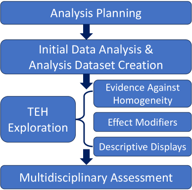
Figure 1: Overview of WATCH workflow and the four main steps: (1) Analysis Planning, (2) Initial Data Analysis and Analysis Dataset Creation, (3) TEH Exploration, and (4) Multidisciplinary Assessment.

In the following sections we will first present the steps above in more detail. To illustrate potential graphical and numerical outputs, we will use simulated data. To this end, we use the benchtm R package [37] to simulate a dataset that mimics clinical trial data. Sun et al. [38] provides details on how the different scenarios are simulated. In our work we will generate a data-set data using Scenario 3, which simulates $n=500$ patients, with $p=30$ baseline variables, out of which two are treatment effect modifiers ($X_{1}$ and $X_{14}$), with a relatively strong treatment effect heterogeneity (i.e. $\beta_{1}$/$\beta_{1}^{*}=2.0$). The data and code used in the paper will be made available in a GitHub repository.

2.1 Analysis Planning

For analysis planning, it is essential to be familiarized with drug, disease and past (or possibly ongoing or planned) clinical trials, as well as engage with the project team and stakeholders. If possible, the planning of the analysis should take place prospectively, before data base lock. It is critical to understand the planned estimands (ICH E9 (R1) Addendum [25]) and analyses, important prognostic factors (stratification and adjustment factors affecting the outcome variable independent of treatment) and the potential treatment effect modifiers (i.e. pre-specified exploratory subgroups). The scientific literature (same drug in other indications; different drugs with the same mechanism in the same indication) may reveal further prognostic variables or potential effect modifiers.

It is crucial to engage with analysis stakeholders and subject-matter experts to confirm that the aim of the analysis is to obtain an overview of how the treatment effect (that is the difference/ratio between two treatments) descriptively varies according to baseline covariates. Similar questions are often around prognostic modelling (risk modelling) of the outcome or cluster analysis in terms of baseline characteristics, which are out of scope for this workflow. Sometimes, the interest at outset might be to identify a subgroup with an enhanced, reduced or no treatment effect.

As a next step, it is necessary to align on the outcome variable(s), study/studies and baseline covariates to include. Regarding the outcome variable, one may be interested in one main outcome variable or a small number of important outcome variables. In case multiple outcome variables are of interest, the analysis below would be repeated for each outcome variable. Findings are more convincing when replicated over several outcome variables (obviously replication of results over highly correlated outcomes is less convincing). Often it also makes sense to perform a sensitivity analysis for modifications of the original outcome variable of interest (e.g., for variables measured over time, using a different time-point, or averaging over time-points).

The next step is to determine the scale of treatment effect. It is well known that the amount and even the existence of treatment effect heterogeneity depends on the treatment effect scale utilized [28, 47]: Treatment effects may be homogeneous on one scale (e.g. relative ratio scale), but not on another scale (e.g. absolute difference scale): For example homogeneous treatment effects on a relative scale (e.g., risk ratio) will automatically be heterogenous on the difference scale (e.g., risk difference) as soon the outcome in the control group varies with patient covariates. The first scale to consider would typically be the one on which treatment effects for the endpoint is commonly presented (often a relative scale). Benefit-risk analyses, however, typically present treatment effects on a absolute difference scale, so that potentially multiple scales need to be considered.

If multiple studies are available, pooling can be considered. There are several pros and cons: A pooled analysis will have a larger sample size and thus potentially more information on treatment effect modifiers. On the other hand one must consider the similarities and differences of the studies to be pooled (method of data collection and definition of endpoint, dose, duration, population, how contemporaneous the studies are,…). In particular the relationship of baseline covariates to outcome and treatment effect (and thus treatment effect modifiers) could be different across trials. In this setting a pooled analysis could be misleading. When pooling is performed it is important to consider baseline population differences across trials (and arms) in particular if a treatment is only available in some of the studies (this then also needs to be appropriately acknowledged in the analysis). When a pooled analysis is performed, it typically makes sense to also repeat the analysis separately by study.

A further crucial step is to determine the baseline variables to use in the analysis. These variables could be

• factors of high plausibility, related to the mechanism of action of the drug, the severity or progression of the disease, or disease subtype

• variables used as part of the design or pre-specified analysis such as stratification variables or baseline value for continuous outcomes or other adjustment factors

• basic demographic information such as age, sex, race/ethnicity and weight

• an established prognostic/risk score.

Similar as recommended in the EMA [14] guideline, it is recommended to document the level of external, a-priori evidence for treatment effect modification. We propose to use the categories none, low, moderate, high for each variable, see Appendix A.1 for details. We anticipate that the most common used category will be low. For the (typically rare) categories moderate and high, a reference to the information source should be provided and documented, as well as the expected direction of the treatment effect. Ideally this takes place before any study or subgroup results were communicated. If the categorization happens afterwards an unbiased representation of a-priori evidence is no longer possible. We nevertheless recommend to categorize variables according to the study external evidence. Often this exercise would result in less than 10-15 covariates. It is an option to repeat the analysis based on a wider set of variables. Analysis results for this more wider set of covariates need to be critically assessed, as the number and plausibility of the included covariates has an important impact on the reliability of conclusions [38]: When one searches for a needle in the haystack, adding hay won’t usually help.

2.2 Initial Data Analysis (IDA) and Analysis Dataset Creation

This step includes two parts: initial data analysis (IDA) and analysis dataset creation. IDA describes the population distribution and covariate dependence. Based on that, one can further preprocess the original data (as discussed in Section 2.1) to generate an analysis dataset.

Initial Data Analysis
The aim of IDA is to explore the variables included in the analysis data sets to familiarize with the data and also to suggest transformation or omission of certain covariates. The main analysis question around treatment effect heterogeneity should not be approached in this step [3]. Our IDA encompasses four steps, and a snapshot of plots that could result from this analysis are displayed in Figure 2.

We recommend to first investigate the distribution for each covariate via histogram or bar plots (Figure 2(a)). This step checks unusual patterns that may appear in the data distribution, such as imbalance between classes, skewed distributions, extreme observations etc. In the second step we produce summary visualizations of the covariates stratified by study and treatment (Figure 2(b)). We recommend this step to check differences in the distributions among different factor levels, across studies or treatment arms in the same study. In the third step, we recommend to investigate missing values (Figure 2(c)) and non-informative covariates. In terms of missing values, we recommend to check the percentage of missingness for each covariate, and the missing pattern across variables. Non-informative covariates can be categorical variables that are concentrated on essentially one factor level. In the final step we recommend analyzing the dependency among covariates by checking pairwise correlation and hierarchical clustering based on the correlations (Figure 2(d)). This helps to identify identical or highly correlated variables and can also guide interpretation of results later. The selection of covariates to be kept usually needs to be discussed with the project team to make sure the most relevant and informative ones are retained.

Analysis Dataset Creation
After initial data analysis, certain changes need to be made to create the analysis dataset, such as variable transformations (for highly skewed covariates, or merging sparse categories for categorical variables), variable omissions (highly dependent covariates or non-informative variables) or imputation of missing baseline covariates. For imputing missing values in the covariates we suggest the imputation of baseline covariates to be independent of outcome or any other post-baseline variables. A variety of approaches are available for this purpose. We encourage users to run analysis with different imputation methods for a robustness check.

For intercurrent events and missing data in the outcome variable we propose (for consistency) to follow the analytical strategy used in the main pre-specified clinical trial analyses for this endpoint, on the decided intercurrent event strategies and missing data handling approaches (see ICH E9 (R1) Addendum [25]). In situations where these approaches are complex (e.g. various multiple imputation strategies used) subsequent analyses for predictive variable identification may become time-consuming and infeasible. In this case we suggest to use simpler approaches that are still in the spirit of the main estimand targeted in the clinical trial analyses. This may often imply using single imputation approaches.

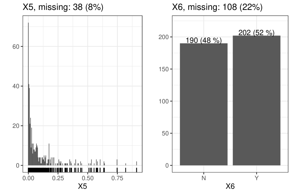
(a) Univariate summaries

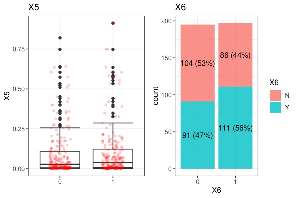
(b) Variables stratified by further factors

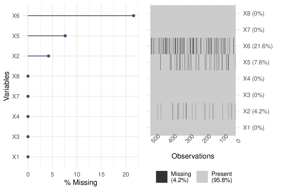
(c) Missing values

(d) Dependence analysis

Figure 2: Various visualisations generated after the Initial Data Analysis (IDA).

2.3 Exploring TEH

The exploration of TEH is the core analytical step of the proposed workflow. We propose to implement this by addressing three questions:

1. How strong is the evidence against homogeneity?

2. Which are the observed effect modifiers?

3. How does the treatment effect change for the identified covariates?

Note that we recommend to structure the effort according to the three questions above; but different modelling approaches can be used for this purpose. An example would be to use (penalized) regression models. Based on this, for (Q1) a global interaction test could be performed and for (Q2) a ranking based on the standardized model coefficients could be presented. Sun et al. [38] performed simulations to compare several statistical methods on their performance to answer the above questions. For illustration, here we use an implementation on the double robust (DR) learner [26] combined with the conditional random forest [24]. The methodological details are not the main topic for this paper, and provided in Appendix A.4. The DR learner is attractive, as it provides a pseudo observation that can be seen as an observation of the treatment effect for each individual. Based on these pseudo observations, one can then directly model the treatment effect in relation to baseline covariates (similar as proposed in the virtual twins approach [15]). As a consequence, the covariates that interact with treatment can be directly identified from the model without modeling main effects. This set up can be used to address all three questions stated above.

Evidence Against Homogeneity
Clinical trials are usually planned in a specific overall population with prior expectation of largely consistent treatment effects across that population (i.e. treatment effect homogeneity). Otherwise, the inclusion criteria of the trial and its primary analysis would have been different.

It is thus a relevant question to ask: “How likely is it to observe the actually observed heterogeneity under a model that uses homogeneous treatment effects?”, while taking into account the number of variables utilized for assessing TEH. Answering this questions also provides useful information with respect to the reliability of possible observed heterogeneous treatment effects: If there is low evidence overall for treatment effect modification, identification of effect modifiers will be less reliable, and the estimation of their effects difficult and prone to random high or random low bias. A number of authors consider a global heterogeneity (global interaction test) as important: Interaction test are prominently mentioned in some of the workflows in the introduction [35, 27, 44]. Chernozhukov et al. [10] propose a machine learning approach to test for global effect modification, which is implemented in the grf R package [40] for the causal forest algorithm. Harrell [21] proposes to use a global likelihood ratio test based on regression models, comparing a model with a treatment indicator and all baseline covariates as main effects, as well as interactions with treatment, to a model that includes only all baseline covariates and treatment as main effects. The PSI/EFSPI Working Group on Subgroup Analysis proposed the Standardised Effects Adjusted for Multiple Overlapping Subgroups (SEAMOS) plot. SEAMOS is intended to provide a graphical presentation of the treatment effects for all pre-specified subgroups to illustrate how extreme/surprising the observed results are if data were generated by a homogeneous treatment effect model [12]. Callegaro et al. [9] compare different options for global interaction tests in the context of clinical trials, when there are high-dimensional covariates.

The resulting p-value from such a global interaction test should not be interpreted as a binary decision rule but on a continuum. Trials are not planned for such tests and the statistical properties of such a decision rule would not be adequate for binary decision making [18]. A high p-value indicates compatibility, while a low p-value indicates contradiction of the data to a model of homogeneous treatment effects. The p-value should be interpreted as measuring the compatibility of the observed data with a model of homogeneous treatment effects [11], see Appendix A.2 for proposed arbitrary verbal descriptions of the level of evidence against homogeneity. The global interaction p-value also provides a metric that can be compared across different situations (e.g., different trials, endpoints, different total number of covariates used).

For the DR learner, the test against homogeneity of treatment effect is equivalent to testing whether the pseudo observation (of individual treatment effect) is independent of baseline covariates. For this purpose we use an independence test as implemented in Hothorn et al. [23]; more details can be found in Appendix A.4. For the simulated data described earlier using this global heterogeneity test based on the DR learner, the p-value is $0.19$, indicating a moderate evidence against homogeneity.

Effect modifiers
Description of the baseline covariates that are most associated with the treatment effect in the observed data is essential. Variable importance can be used to determine the contribution of baseline variables towards treatment effects. However, there is no standard method for defining variable importance, and the implementation of variable importance calculation can vary [45]. One established approach is permutation importance, which involves permuting the covariates and measuring the increase in the prediction error of the model [6]. This importance measure is model agnostic and can be more easily implemented to compare the performance between different models. Variable importance derived from permutation importance represents multivariate importance, which measures the contribution of one covariate, with other covariates in the model. Other than exploring the variable importance for each covariate, one could also consider the variable importance based on paired variable contribution, see Molnar [30] for more discussion on this topic.

Figure 3 (a) presents the permutation importance based on conditional random forests [24] for the simulated data. Figure 3 (b) presents the interaction (permutation variable importance is displayed on the diagonal) variable importance [19]. This figure helps to narrow down the variables of interest for further exploration. For the observed data $X_{1}$ is most strongly associated with the treatment effect (which we know is correct), while the other true treatment effect modifier ($X_{14}$) does not appear to be highly associated with the treatment effect in the simulated data.

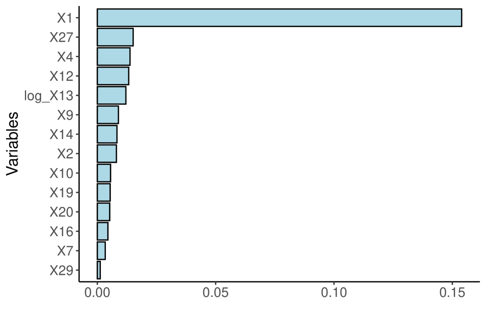
(a) Permutation Variable importance

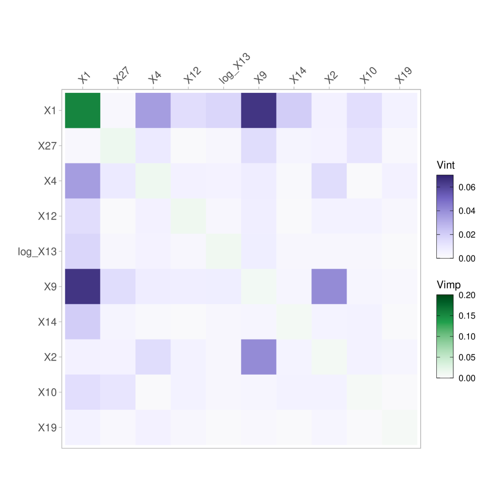
(b) Interaction variable importance

Figure 3: Two different visualisations for the variable importance that captures the contribution of baseline variables towards treatment effects.

Descriptive display of TEH
In order to investigate the covariates that appear high in the ranking, we recommend to present visualizations of how the treatment effect changes with respect to these covariates. This can be done in a univariate way, or in a bivariate way, i.e. checking pairs of variables. Furthermore, we propose to provide plots with the per arm response, and with the corresponding treatment effect. Please refer to the snapshot of these visualization plots in Figure 4 and Figure 5.

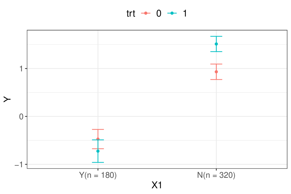
(a)

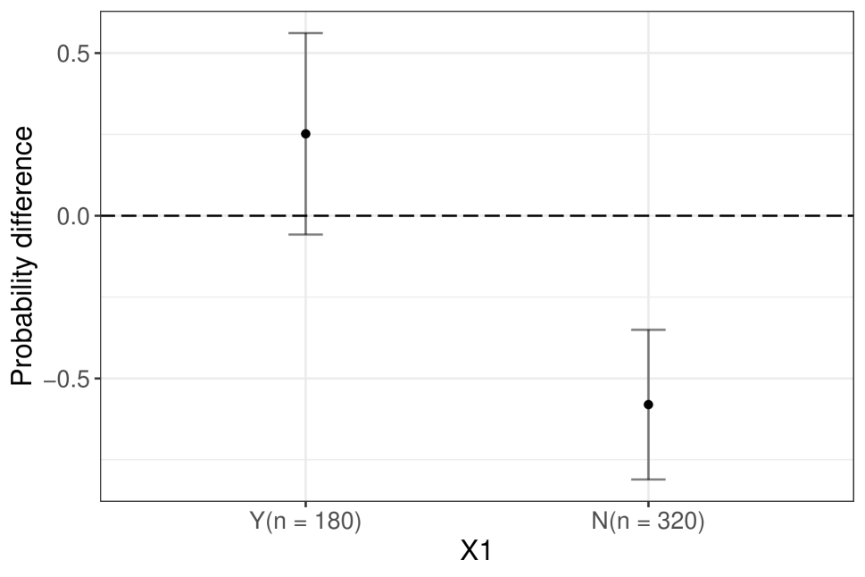
(b)

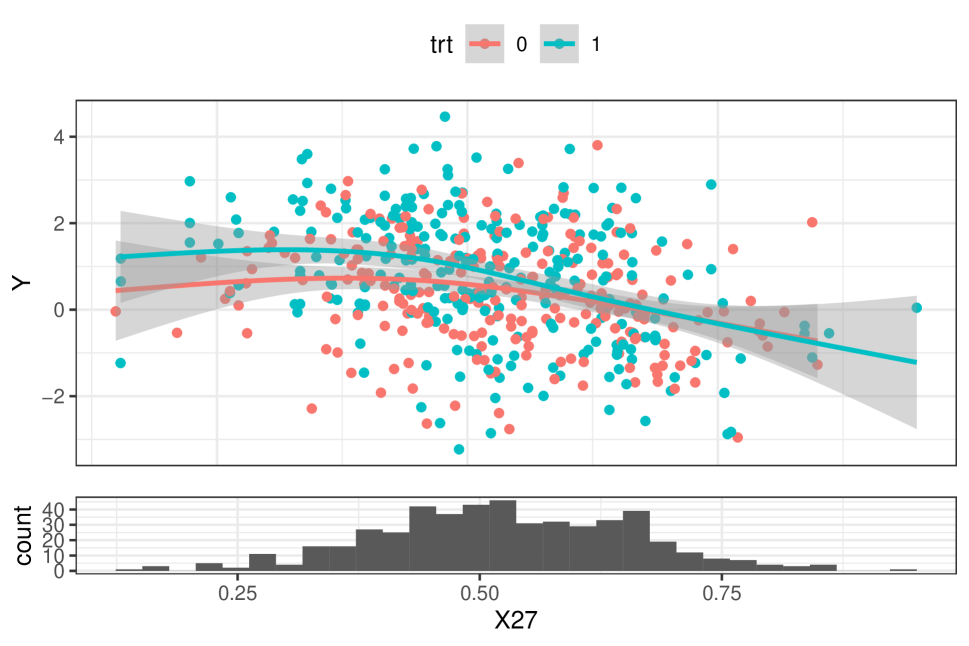
(c)

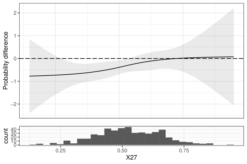
(d)

Figure 4: Univariate display of outcome/treatment effect. Panel (a) shows the outcome mean and associated confidence intervals using data within each group of $X_{1}$. In Panel (c) the curve (with shaded pointwise 95% confidence interval) is displayed in dependence on the covariate X27, estimated using a Generalized Linear Model (GLM) with a regression spline. Furthermore, Panels (b) and (d) provide the corresponding plots for the treatment effects. Furthermore, Panels (b) and (d) provide the corresponding plots for the treatment effects.

Figure 4 illustrates the covariates (use $X_{1}$ and $X_{27}$ for demonstration) and treatment effects/outcomes. Panels (a) and (c) depict the impact of the covariates (categorical covariate in Panel (a) and continuous covariate in Panel (c)) on outcomes in different treatment arms (green for treated arm and red for placebo arm), while ignoring other covariates. These plots demonstrate the marginal effect of the corresponding covariates. The histogram of covariates (bottom subpanel from Panel (c))) and total number of patients in each group (from Panel (a))) provide information on the amount of data for interpretation. In addition to the outcome plots based on the covariates of interest, it is useful to provide corresponding plots for treatment effects as a comparison (Panels (b) and (d)).

Aside from univariate plots, bivariate plots are also crucial in providing insights into the interaction effect of two covariates on treatment effects (see Figure 5). These types of plots enable to comprehend how the contribution of one covariate to treatment effects varies at different levels of the other covariate. Panel (a) of Figure 5 demonstrates patient outcomes on treatment (green) and placebo (red) arms at different levels of combinations of $X_{1}$ and $X_{9}$ (which has a high interaction importance, see Figure 3 Panel (b)). For each subpanel, the point estimation (with confidence interval) is estimated in the same way as in Figure 4, stratified by the second variable. Similarly, Panel (b) demonstrates the relationship between two covariates and their contribution to treatment effects. Similarly continuous variables would be displayed as in Figure 4 with regression splines, but stratified by the second variable. Because now the overall data are subset according to two variables, the conclusions get more variable and hence unreliable. Appendix A.3 provides information on the correlation of the 10 baseline variables that have the largest variable importance.

As the overall interaction p-value here only indicated a moderate evidence against homogeneity the results in these plots would need to be cautiously interpreted. In fact, while the variables $X_{1}$ and $X_{9}$ interact strongly in the observed data on the treatment effect, this is not the case for the data generating model.

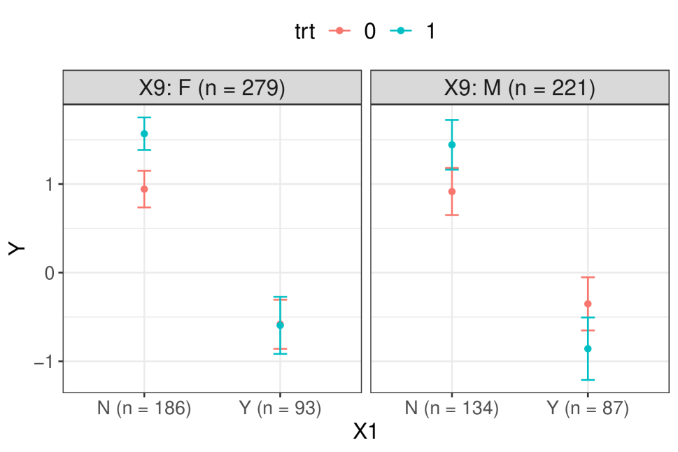
(a)

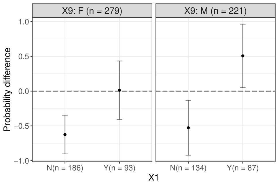
(b)

Figure 5: Bivariate display of outcome/treatment effect. Panel (a) shows the outcome mean and associated confidence intervals using data within all possible groups defined by X1 and X9 jointly. Panel (b) provides the corresponding plot for the treatment effects.

It is a conscious choice that these plots show observed data and/or simple summaries (means and regression splines) only and not results summarising a model fit (based on the conditional random forest in this case). An alternative display would be model-based partial dependence plots [16] that investigate the effect of a baseline variable on the outcome independent of other variables, by effectively breaking correlations of the observed baseline variables for the display (using a form of standardization). This identifies which baseline variables are the drivers of heterogeneity for correlated variables. In our workflow this task is achieved by the model-based variable importance measure, but for display it is considered more appropriate to show the observed data and outcome means with the correlations as they appear in the data, which is more practically relevant (as correlations across baseline variables cannot be removed in the real world).

In addition to the bivariate plots, exhaustive subgroup plots [31] also provide a useful method for obtaining an overview of how treatment effects vary across subgroups; they have the appealing feature of putting the observed treatment effects into the context of many other subgroup treatment effects.

In summary, we want to highlight that one of the goals of WATCH workflow is to provide an overview of treatment effect heterogeneity and enhance our knowledge of the data by using visualizations and descriptions, and to present the data in the most comprehensive way so better decisions can be taken.

2.4 Multidisciplinary Assessment

As discussed in Section 1, the data-driven results obtained need to be assessed for credibility in light of existing external data and best scientific understanding. This is best achieved in a multidisciplinary discussion.

The results from the workflow are descriptive and intended to be hypothesis-generating. Thus, strong inferential statements should be avoided when the results are communicated. The global interaction p-value(s) serve an overall diagnostic measure that guides on how much weight should be put on results that follow, such as variable importance and treatment effect plots. The focus should be on a global overview instead of selective reporting of a single finding. To interpret the findings it is crucial to revisit the list of variables specified before start of the investigation as well as their external evidence and expected direction of the treatment effect. Data-driven findings that are not supported by a-priori, external evidence (categories none and to some degree low external evidence, see Appendix A.1) are of low credibility in particular if the global interaction p-value is large. On the other hand, strong findings with high external and a-priori evidence and correct pre-defined direction of treatment effect, should be considered very notable in particular when the global interaction p-value is smaller.

If further robustness analyses were conducted, then results could be mentioned and the focus should be on the similarities and differences in results compared to the main analysis. Robustness analyses could be with respect to using different endpoint, different time-point for the same endpoint, different covariate set, performing analyses by study if multiple studies are involved, using different missing data imputation methods, using different treatment effect scales (e.g. relative versus absolute).

Based on the information provided, the development team could consider different steps, depending on the drug development context: If the overall evidence and credibility of findings is low, this is useful strategic information, and the decision may be to nevertheless observe specific variables more closely in potential follow-up trials. In other cases where there is credibility for some of the findings, one might do further investigations to understand better the factors that could have caused the heterogeneity. In this case the investigation and analyses could be published externally and/or provide supportive information in health authority interactions. It is also possible that the team may be interested in identifying a specific subgroup as part of this discussion. This goes beyond this workflow, as it also depends on trade-offs that may need further stakeholder discussion (e.g.trade-off of subgroup size versus subgroup treatment effect; trade-off of subgroup efficacy versus subgroup safety). In this more inferential context, we suggest using methodologies such as shrinkage estimation of treatment effects to protect against random high selection bias, for example when making the choice on the treatment effect a new trial should be sample-sized for (see Thomas and Bornkamp [39] and Riehl et al. [32]).

3 Conclusions

Understanding how treatment effect varies across patients may influence important sponsors decisions, related to drug development. Decisions on these aspects are based on internal exploratory analyses, which is challenging as clinical trials are not formally planned to investigate heterogeneity. This highlights the need to take into account existing external data and best scientific understanding. In this paper we proposed a workflow to describe and interpret treatment effect heterogeneity for trial sponsors in this non-inferential/exploratory setting [41, 31].

The core analytical part of the workflow consists of (i) an assessment of the global evidence against heterogeneity (according to the utilized covariates), (ii) providing a variable importance measure describing which baseline covariates are most associated with the treatment effect, and (iii) descriptive displays of how the treatment effect varies according to the important covariates. Assessment of the credibility of data-driven findings is facilitated due to an a-priori classification of the utilized baseline variables by external evidence and a final multidisciplinary assessment. Taking into account external information is consistent with the EMA guideline for subgroup analyses [14].

In current practice, supportive, prespecified subgroup analyses are produced by default for important clinical trials and typically displayed in forest plots. In addition purely post-hoc exploratory analyses are performed (e.g. based on flexible statistical modeling and/or machine learning). While both approaches provide an overview of treatment effect heterogeneity, we believe the proposed workflow improves upon this:

• It provides an overall assessment of evidence against homogeneity (rather than just univariate for each variable/subgroup in the forest plot), taking into account the number of utilized covariates (multiplicity).

• It is based on a multivariate assessment due to the chosen variable importance measures [20], allowing to better understand the true drivers for heterogeneity, when there are correlated variables.

• It does not require to dichotomize continuous baseline covariates and more covariates can be assessed compared to the forest plot.

• It allows to investigate on how two covariates interact on the treatment effect (which is usually not considered in a forest plot).

• It provides a systematic approach to summarize a-priori external evidence for treatment effect modification for each variable including a categorization of the corresponding evidence, which helps an assessment of credibility.

• Compared to more post-hoc exploratory analyses its results can be quickly be available after data-base lock, due to the pre-planning.

While in subgroup analysis and treatment effect heterogeneity literature most of the works focus on developing and evaluating analytical techniques, in our paper we wanted to emphasize that this is only one part in the work of a statistician or data scientist. The proposed WATCH workflow, that follows the PPDAC model, provides a systematic approach to explore treatment effect heterogeneity in the exploratory setting, taking into account external evidence and best scientific understanding. It has the potential to increase decision making around treatment effect heterogeneity and therefore suggest to plan for such an activity routinely at the time of design of any (sufficiently large) clinical trial. The importance of using structured problem-solving frameworks, such as PPDAC, to approach these exploratory endeavors has been highlighted in statistics literature [46, 36], and in biopharmaceutical research [7].

As we emphasized, our workflow focuses on the non-inferential/exploratory setting. For inferential subgroup identification a different workflow would be required, although some steps can be similar (e.g. analysis planning, deciding on the considered covariates and the existing a-priori/external evidence, the IDA and the analysis dataset creation). In inferential workflow considerations are needed for interpreting a positive subgroup finding in the presence of an overall treatment effect finding, whether that finding is positive or negative. This is a topic of further research and consideration.

Appendix A Appendix

A.1 A-priori categorization of the level external evidence

We propose the following categorization of the level of external evidence for effect modification for specific variables.

• The none category should be used for variables that are included for reasons unrelated to plausibility or external evidence, but there is interest to investigate whether there is effect modification (depending on the context this could be variables such as age, sex or race). If a variable in this category comes up high in the importance ranking, this needs to be cautiously interpreted.

• The low category is the default category, as it is expected that included variables are considered as plausible effect modifiers, but most of the time without additional external evidence.

• In case there is documented external / a priori evidence for the modification of the treatment effect for a baseline variable (e.g., study external data or presentation/publication), but it is not clear how relevant or reliable this evidence is, the moderate category should be used.

• The high category should only be used when there exists strong directly relevant evidence that a variable will be a treatment effect modifier. It is expected that high will be very rarely applicable (otherwise, the underlying studies would have been designed in a different way).

For the categories moderate and high, a reference to the information source should be provided and documented, as well as the expected direction of the treatment effect.

A.2 Verbal summary of level of evidence against homogeneity

Table 1 provides a verbal summary of level of evidence against homogeneity. The suggested scale for assessing evidence is based on the surprise value [11], which is given by logarithm of base 2 of the p-value. It has a nice interpretation, since it represents the number of consecutive coin-flips with all heads up, under the hypothesis of a fair coin.

	surprise value	verbal summary of
p-value	($\log_{2}(p)$)	evidence against homogeneity
$[0.25,1]$	$(0,2]$	low
$[0.063,0.25)$	$(3,4]$	moderate
$[0.008,0.063)$	$(5,7]$	noteworthy
$[0.001,0.008)$	$(8,10]$	strong
$<0.001$	$>10$	very strong

Table 1: Suggested verbal summary of level of evidence against homogeneity.

A.3 Correlation of baseline variables in simulated data

For the top 10 identified baseline covariates (based on variable importance), the density/bar plot for each variable, as well as the correlation (scatterplot/boxplot/bar plot) between each pair of variables are shown in Figure 6.

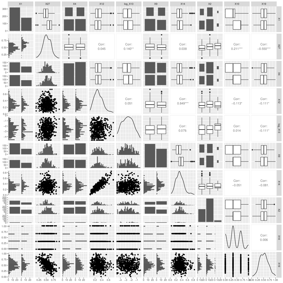
Figure 6: Correlation of selected variables in the simulated data-set.

A.4 Details on the double-robust learner for example data

In this section we provide more details on the DR-learner [26] and how it was used in the presented example. Assume we have an i.i.d. sample of observations of $Z_{i}=(X_{i},A_{i},Y_{i})$, where $X\in\mathbb{R}^{p}$ are covariates, $A\in\{0,1\}$ is a binary treatment, and $Y\in\mathbb{R}$ an outcome of interest. We denote as $Y^{1}$ the potential outcome that would have been observed if the patient was receiving the treatment $A=1,$ while as $Y^{0}$ if the patient was receiving the treatment $A=0.$ The DR learner is a procedure to estimate the conditional average treatment effect (CATE), $\mathbf{E}(Y^{1}-Y^{0}|X=x)$. For doing this “pseudo-outcomes” are created for each patient, which can be seen as a noisy version of the CATE created. Algorithm 1 provides a detailed description of the construction of the pseudo outcomes for all patients and it is based on an algorithm described by Kennedy [26]. In Algorithm 1 we need to estimate three nuisance functions ($\widehat{\mu}_{0},\widehat{\mu}_{1},\widehat{\pi}$). To this end we can utilize flexible regression models using machine learning. In our work we implement an ensemble of models using the SuperLearner, an algorithm that uses cross-validation to estimate the performance of multiple models, and then creates an optimal weighted average of those models (stacking) using the test data performance [42]. In our case we used penalized regression (LASSO), gradient boosting and random forests as the base learners.

Algorithm 1 DR learner

Let $(D_{1}^{n},...,D_{K}^{n})$ denote K splits of n observations from the overall data based on a k-fold cross-validation. Let $D_{-k}$ denote the union of all cross-validation folds without the k-th fold $D_{k}^{n}$. of $Z_{i}=(X_{i},A_{i},Y_{i}).$

• Step 1.

Nuisance training:

• (a)

Construct estimates $\widehat{\pi}$ of the propensity scores $\pi(X)=\mathbf{P}(A=1|X)$ using $D_{-k}$.

• (b)

Construct estimates $\widehat{\mu}_{0},\widehat{\mu}_{1}$ of the regression functions ${\mu}_{A}(X)=\mathbf{E}(Y|X,A)$ using $D_{-k}$.

• Step 2.

Pseudo-outcome: Construct the pseudo-outcome for all patients $i$ in $D_{k}^{n}$

$$\widehat{\phi}(X_{i})=\frac{A_{i}-\widehat{\pi}(X_{i})}{\widehat{\pi}(X_{i})\{1-\widehat{\pi}(X_{i})\}}\{Y_{i}-\widehat{\mu}_{A_{i}}(X_{i})\}+\widehat{\mu}_{1}(X_{i})-\widehat{\mu}_{0}(X_{i})$$ (1)

Iterating steps 1 and 2 for all $K$ folds, This will provide a pseudo-outcome $\widehat{\phi}(X_{i})$ for all patients.

Using pseudo-observations in a second step for inference for the treatment effect is convenient, because standard methods for modelling or regression can be used directly on the pseudo observations, without the need to model both main effects and interactions with treatment. As part of our workflow we don’t directly need to estimate CATE, but are interested (i) in the evidence against homogeneity and (ii) to determine the treatment effect modifiers. To assess the evidence against homogeneity, we use the pseudo-observations to perform a global test against the homogeneity. We are interested in testing the following null hypothesis: $H_{0}:\widehat{\phi}(X)\perp\!\!\!\perp X.$ A number of methods can be used to perform that independence test, but in our implementation we use a test based on conditional inference procedures [23]. To answer the question on the important effect modifiers, we use again the pseudo-observations. To do that in a multi-variate fashion, we use the data $(X_{i},\widehat{\phi}(X_{i}))$ to build a conditional random forest model, and then rank the different covariates on their variable importance score. Because the clinical variables are of mixed data (continuous and categorical) it is important not to have any selection bias towards covariates with many possible splits. In our work implementation we use conditional inference trees [24], an unbiased recursive partitioning method.

Appendix B Acknowledgement

The authors would like to thank Frank Bretz, Malika Cremer and Peter Quarg for their feedback and discussion on earlier versions of the manuscript.

References

- [1] M. Alosh, M. F. Huque, F. Bretz, and R. B. D’Agostino Sr. Tutorial on statistical considerations on subgroup analysis in confirmatory clinical trials. Statistics in medicine, 36(8):1334–1360, 2017.
- [2] A. K. Amatya, M. H. Fiero, E. W. Bloomquist, A. K. Sinha, S. J. Lemery, H. Singh, A. Ibrahim, M. Donoghue, L. A. Fashoyin-Aje, R. A. de Claro, et al. Subgroup analyses in oncology trials: regulatory considerations and case examples. Clinical Cancer Research, 27(21):5753–5756, 2021.
- [3] M. Baillie, S. le Cessie, C. O. Schmidt, L. Lusa, M. Huebner, and T. G. I. D. A. of the STRATOS Initiative. Ten simple rules for initial data analysis. PLoS Computational Biology, 18(2):e1009819, 2022.
- [4] M. Baillie, C. Moloney, C. P. Mueller, J. Dorn, J. Branson, and D. Ohlssen. Good data science practice: Moving toward a code of practice for drug development. Statistics in Biopharmaceutical Research, 15(1):74–85, 2023.
- [5] B. Bornkamp, S. Zaoli, M. Azzarito, R. Martin, C. P. Müller, C. Moloney, G. Capestro, D. Ohlssen, and M. Baillie. Predicting subgroup treatment effects for a new study: Motivations, results and learnings from running a data challenge in a pharmaceutical corporation. Pharmaceutical Statistics, 2024.
- [6] L. Breiman. Random forests. Machine learning, 45:5–32, 2001.
- [7] F. Bretz and J. B. Greenhouse. The role of statistical thinking in biopharmaceutical research. Statistics in Biopharmaceutical Research, 15(3):458–467, 2023.
- [8] F. Bretz and P. H. Westfall. Multiplicity and replicability: two sides of the same coin. Pharmaceutical statistics, 6(13):343–344, 2014.
- [9] A. Callegaro, B. Spiessens, B. Dizier, F. U. Montoya, and H. C. van Houwelingen. Testing interaction between treatment and high-dimensional covariates in randomized clinical trials. Biometrical Journal, 59(4):672–684, 2017.
- [10] V. Chernozhukov, M. Demirer, E. Duflo, and I. Fernández-Val. Generic machine learning inference on heterogenous treatment effects in randomized experiments. arXiv preprint arXiv:1712.04802, 2017.
- [11] S. R. Cole, J. K. Edwards, and S. Greenland. Surprise! American Journal of Epidemiology, 190(2):191–193, 07 2020.
- [12] A. Dane, A. Spencer, G. Rosenkranz, I. Lipkovich, T. Parke, and P. W. G. on Subgroup Analysis. Subgroup analysis and interpretation for phase 3 confirmatory trials: White paper of the efspi/psi working group on subgroup analysis. Pharmaceutical Statistics, 18(2):126–139, 2019.
- [13] A. Dmitrienko, C. Muysers, A. Fritsch, and I. Lipkovich. General guidance on exploratory and confirmatory subgroup analysis in late-stage clinical trials. Journal of biopharmaceutical statistics, 26(1):71–98, 2016.
- [14] European Medicines Agency. Guideline on the investigation of subgroups in confirmatory clinical trials. EMA/CHMP/539146, 2019.
- [15] J. C. Foster, J. M. Taylor, and S. J. Ruberg. Subgroup identification from randomized clinical trial data. Statistics in medicine, 30(24):2867–2880, 2011.
- [16] J. H. Friedman. Greedy function approximation: a gradient boosting machine. Annals of statistics, pages 1189–1232, 2001.
- [17] A. Gelman, J. Hill, and A. Vehtari. Regression and other stories. Cambridge University Press, 2020.
- [18] S. Greenland. Divergence versus decision p-values: A distinction worth making in theory and keeping in practice: Or, how divergence p-values measure evidence even when decision p-values do not. Scandinavian Journal of Statistics, 50(1):54–88, 2023.
- [19] B. M. Greenwell, B. C. Boehmke, and A. J. McCarthy. A simple and effective model-based variable importance measure. arXiv preprint arXiv:1805.04755, 2018.
- [20] B. Gregorutti, B. Michel, and P. Saint-Pierre. Correlation and variable importance in random forests. Statistics and Computing, 27:659–678, 2017.
- [21] F. Harrell. Biostatistics for biomedical research, 2023. Section 13.6 under https://hbiostat.org/bbr/ (accessed September 25, 2023).
- [22] R. Hemmings. An overview of statistical and regulatory issues in the planning, analysis, and interpretation of subgroup analyses in confirmatory clinical trials. Journal of biopharmaceutical statistics, 24(1):4–18, 2014.
- [23] T. Hothorn, K. Hornik, M. A. Van De Wiel, and A. Zeileis. A lego system for conditional inference. The American Statistician, 60(3):257–263, 2006.
- [24] T. Hothorn, K. Hornik, and A. Zeileis. Unbiased recursive partitioning: A conditional inference framework. Journal of Computational and Graphical statistics, 15(3):651–674, 2006.
- [25] International Council For Harmonisation of Technical Requirements For Pharmaceuticals For Human Use (ICH). ICH E9(R1) addendum on estimands and sensitivity analysis in clinical trials to the guideline on statistical principles for clinical trials, 2019. Accessible via ”https://database.ich.org/sites/default/files/E9-R1_Step4_Guideline_2019_1203.pdf”.
- [26] E. H. Kennedy. Towards optimal doubly robust estimation of heterogeneous causal effects. Electronic Journal of Statistics, 17(2):3008–3049, 2023.
- [27] D. M. Kent, J. K. Paulus, D. Van Klaveren, R. D’Agostino, S. Goodman, R. Hayward, J. P. Ioannidis, B. Patrick-Lake, S. Morton, M. Pencina, et al. The predictive approaches to treatment effect heterogeneity (path) statement. Annals of internal medicine, 172(1):35–45, 2020.
- [28] D. M. Kent, D. Van Klaveren, J. K. Paulus, R. D’Agostino, S. Goodman, R. Hayward, J. P. Ioannidis, B. Patrick-Lake, S. Morton, M. Pencina, et al. The predictive approaches to treatment effect heterogeneity (path) statement: explanation and elaboration. Annals of internal medicine, 172(1):W1–W25, 2020.
- [29] I. Lipkovich, A. Dmitrienko, and R. B. D’Agostini. Tutorial in biostatistics: data-driven subgroup identification and analysis in clinical trials. Statistics in Medicine, 36(1):136–196, 2017.
- [30] C. Molnar. A guide for making black box models explainable. URL: https://christophm. github. io/interpretable-ml-book, 2(3), 2018.
- [31] C. Muysers, A. Dmitrienko, H. Kulmann, B. Kirsch, S. Lippert, T. Schmelter, A. Schulz, N. Mentenich, H. Schmitz, M. Schaefers, et al. A systematic approach for post hoc subgroup analyses with applications in clinical case studies. Therapeutic innovation & regulatory science, pages 1–12, 2020.
- [32] J. Riehl, A. Fritsch, and K. Ickstadt. Shrinkage estimation methods for subgroup analyses. Statistics in Biopharmaceutical Research, 15:755–766, 2022.
- [33] S. J. Ruberg. Assessing and communicating heterogeneity of treatment effects for patient subpopulations: The hardest problem there is. Pharmaceutical Statistics, 20(5):939–944, 2021.
- [34] S. J. Ruberg and L. Shen. Personalized medicine: Four perspectives of tailored medicine. Statistics in Biopharmaceutical Research, 7:214–229, 2015.
- [35] S. Schandelmaier, M. Briel, R. Varadhan, C. H. Schmid, N. Devasenapathy, R. A. Hayward, J. Gagnier, M. Borenstein, G. J. van der Heijden, I. J. Dahabreh, X. Sun, W. Sauerbrei, M. Walsh, J. P. Ioannidis, L. Thabane, and G. H. Guyatt. Development of the instrument to assess the credibility of effect modification analyses (iceman) in randomized controlled trials and meta-analyses. CMAJ, 192(32):E901–E906, 2020.
- [36] D. Spiegelhalter. The art of statistics: Learning from data. Penguin UK, 2019.
- [37] S. Sun, B. Bornkamp, J. Lu, A. Mirshani, K. Sechidis, and Y. Chen. benchtm, 2022.
- [38] S. Sun, K. Sechidis, Y. Chen, J. Lu, C. Ma, A. Mirshani, D. Ohlssen, M. Vandemeulebroecke, and B. Bornkamp. Comparing algorithms for characterizing treatment effect heterogeneity in randomized trials. Biometrical Journal, 2022.
- [39] M. Thomas and B. Bornkamp. Comparing approaches to treatment effect estimation for subgroups in clinical trials. Statistics in Biopharmaceutical Research, 9(2):160–171, 2017.
- [40] J. Tibshirani, S. Athey, E. Sverdrup, and S. Wager. grf: Generalized Random Forests, 2023.
- [41] C. Tong. Statistical inference enables bad science; statistical thinking enables good science. The American Statistician, 73:246–261, 2019.
- [42] M. J. Van der Laan, E. C. Polley, and A. E. Hubbard. Super learner. Statistical applications in genetics and molecular biology, 6(1), 2007.
- [43] J. D. Wallach, P. G. Sullivan, J. F. Trepanowski, K. L. Sainani, E. W. Steyerberg, and J. P. Ioannidis. Evaluation of evidence of statistical support and corroboration of subgroup claims in randomized clinical trials. JAMA internal medicine, 177(4):554–560, 2017.
- [44] J. A. Watson and C. C. Holmes. Machine learning analysis plans for randomised controlled trials: detecting treatment effect heterogeneity with strict control of type i error. Trials, 21(1):156, 2020.
- [45] P. Wei, Z. Lu, and J. Song. Variable importance analysis: A comprehensive review. Reliability Engineering and System Safety, 142:399–432, 2015.
- [46] C. J. Wild and M. Pfannkuch. Statistical thinking in empirical enquiry. International statistical review, 67(3):223–248, 1999.
- [47] S. Yusuf and J. Wittes. Interpreting geographic variations in results of randomized, controlled trials. New England Journal of Medicine, 375(23):2263–2271, 2016.
- [48] S. Yusuf, J. Wittes, J. Probstfield, and H. A. Tyroler. Analysis and interpretation of treatment effects in subgroups of patients in randomized clinical trials. JAMA, 266(1):93–98, Jul 1991.