Evolution of Flare Activity in GKM Stars Younger than 300 Myr over Five Years of TESS Observations

Abstract

Stellar flares are short-duration ($<$ hours) bursts of radiation associated with surface magnetic reconnection events. Stellar magnetic activity generally decreases as a function of both age and Rossby number, $R_{0}$, a measure of the relative importance of the convective and rotational dynamos. Young stars ($<300$ Myr) have typically been overlooked in population-level flare studies due to challenges with flare-detection methods. Here, we select a sample of stars that are members of 26 nearby moving groups, clusters, or associations with ages $<$300 Myr that have been observed by the Transiting Exoplanet Survey Satellite (TESS) at 2-minute cadence. We identified 26,355 flares originating from 3,160 stars and robustly measure the rotation periods of 1,847 stars. We measure and find the flare frequency distribution (FFD) slope, $\alpha$, saturates for all spectral types at $\alpha\sim-0.5$ and is constant over 300 Myr. Additionally, we find that flare rates for stars $t_{\textrm{age}}=50-250$ Myr are saturated below $R_{0}<0.14$, which is consistent with other indicators of magnetic activity. We find evidence of annual flare rate variability in eleven stars, potentially correlated with long term stellar activity cycles. Additionally, we cross match our entire sample with GALEX and find no correlation between flare rate and Far- and Near-Ultraviolet flux. Finally, we find the flare rates of planet hosting stars are relatively lower than comparable, larger samples of stars, which may have ramifications for the atmospheric evolution of short-period exoplanets.

1 Introduction

Stellar flares are the radiation component of magnetic reconnection events (Benz & Güdel, 2010). Such events are readily seen on the Sun (Carrington, 1859; Lu & Hamilton, 1991; Fletcher et al., 2011), particularly during the maximum in the solar cycle (Webb & Howard, 1994). Solar flares can be used as proxies for magnetic activity occurring on other stars (Feigelson & Montmerle, 1999; Berdyugina, 2005; Kowalski et al., 2010; Feinstein et al., 2022a). Additionally, these short-duration flaring events can have significant ramifications on the evolution of short-period extrasolar planets (France et al., 2016; Günther et al., 2020; Chen et al., 2021). While stellar flares are typically not spatially resolvable, they do lend themselves to characterization via spectroscopic and photometric signatures. Spectroscopic characterization of stellar flares inform our understanding of non-thermal processes affiliated with such events such as coronal mass ejections (Argiroffi et al., 2019; Vida et al., 2019), proton beams (Orrall & Zirker, 1976; Woodgate et al., 1992), and accelerated electrons (Osten et al., 2005; Smith et al., 2005).

Photometric observations of stars are more readily available now with exoplanet transit discovery missions, and allow us to statistically characterize flare rates and energies at optical/near-infrared wavelengths. Observations of M dwarfs with the Sloan Digital Sky Survey revealed a correlation between the flaring fraction of stars with height above the galactic plane, a proxy for age (Kowalski et al., 2009; Hilton et al., 2010). More recently, NASA’s Kepler, K2, and the Transiting Exoplanet Survey Satellite (TESS) missions have provided a wealth of stellar variability data in addition to their primary objective of detecting transiting exoplanets. Flares can be identified within time-series photometry by a sharp rise and subsequent exponential decay in flux, with the latter corresponding to the cooling rate (Kowalski et al., 2013). Kepler (Borucki et al., 2010) provided long-baseline high-cadence observations used to identify stellar flares. There has been extensive studies of flares in Kepler data, from the statistics of superflares on solar-type stars (e.g. Notsu et al., 2013; Shibayama et al., 2013; Maehara et al., 2015; Okamoto et al., 2021) to low-mass stars (e.g. Hawley et al., 2014; Silverberg et al., 2016). Davenport et al. (2019) found that flare activity decreased with increasing rotation period for 347 GKM stars. However, the flare frequency distribution (FFD) slope did not vary significantly as a function of age. As a caveat, the ages of the stars in this study were determined based on their rotation periods, relying on the assumption that gyrochronology alone accurately ages stars.

K2 provided 70-day baseline observations for a handful of young stars in groups such as Upper Scorpius, Pleiades, Hyades, and Praespe clusters. Ilin et al. (2019, 2021) analyzed flares from K and M stars in these clusters and found that the overall flare activity decreased as a function of age. Moreover, this relationship was steeper for more massive stars in the sample. Paudel et al. (2018) surveyed 10 M6 - L0 dwarfs observed with K2 and found the L0 dwarfs had significantly shallower FFDs than the M dwarfs. They found that, on average, young targets (defined by the tangential velocity of the star) exhibited more flares overall. More recently, TESS (Ricker et al., 2015) has provided near all-sky photometric observations at 30-minute cadence or less. This observing strategy has allowed for more detailed studies of young stellar flares from nearby, disperse young moving groups and associations. These data permit detailed studies of individual stars, for example characterizing eight superflares ($E_{f}>10^{34}$ erg) on the young star AB Doradus over $\sim 60$ days of continuous observations (Schmitt et al., 2019), as well as statistical studies of flares across a range of spectral types and ages (Doyle et al., 2020; Feinstein et al., 2022a; Pietras et al., 2022; Yang et al., 2023b).

The 11-year solar activity cycle represents a change in the magnetic activity of the Sun, and manifests itself in a variety of observables including increases in the total number of sunspots (Clette et al., 2014; Kilcik et al., 2014), flares and coronal mass ejections (Crosby et al., 1993; Webb & Howard, 1994; Lin et al., 2023), and an increase in the total solar irradiance (Lean, 1987). Insights into the long-term activity cycles on other stars have been limited to photometric and spectroscopic monitoring (Saar & Brandenburg, 1999). Lehtinen et al. (2016) collected 16 to 27 years of B- and V-band photometry for 21 young active solar-type stars. They found evidence of long-term stellar activity cycles in 18 targets for which$P_{\textrm{rot}}/P_{\textrm{cycle}}\propto R_{0}^{-1}$, where $P_{\textrm{rot}}$ is the rotation period, $P_{\textrm{cycle}}$ is the period of the stellar activity cycle, and $R_{0}$ is the Rossby number. Additionally, 50 years of spectroscopic observations of HD 166620 from the Mount Wilson Observatory and Keck revealed both a $\sim 16$ year periodicity in emission from the core of the Ca II H and K lines (Oláh et al., 2016) and evidence that this star entered a grand minima (Baum et al., 2022). A more complete review on the state of stellar activity cycles can be found in Jeffers et al. (2023) and Işık et al. (2023).

In addition to photometric and spectroscopic observations, solar flares trace the length of the solar activity cycle. The high-cadence observations from Kepler (4-year baseline) and TESS (currently 5-year baseline) provide sufficient data for searches of stellar activity cycles from the variations in stellar flare rates. Davenport et al. (2020) demonstrated that the flare rate and FFDs of GJ 1234 has not changed appreciably over 10 years of observations with both Kepler and TESS. On the other hand, Scoggins et al. (2019) found that the M3V star star KIC 8507979 showed a clear decline in flare rate and change in FFD over 4-years of Kepler observations. While it is not expected to find flare rate and distribution variations in all stars given detection limitations, KIC 8507979 demonstrates the ability to study long-term flare variability as a potential tracer for stellar activity cycles.

The paper is presented as follows. In Section 2, we describe our sample, and stellar flare and rotation period identification methods. In Section 3, we present our flare-frequency distribution (FFD) fits as a function of stellar age, $T_{\textrm{eff}}$, and $R_{0}$. In Section 4, we present evidence of flare rate changes over the 5-year TESS baseline in eleven young stars, likely correlated with long term stellar activity cycles. In Section 5, we search for correlations in flare rates with FUV and NUV observations from GALEX and place the flare rates of young planet hosting stars in the context of our broader sample. We conclude in Section 6. We provide additional figures and tables in Section A.

This paper was written using the showyourwork! open-source software package. The objective of showyourwork! is to improve reproducibility and transparency of scientific research by compiling the manuscript and figures simultaneously. All of the data in this work is hosted on GitHub and Zenodo. At the end of every caption figure in this manuscript, there is a GitHub icon ( ), which links to the Python script used to create that figure.

2 TESS Light Curve Characterization

Here, we provide an overview of the methodology used in this paper. Specifically, we describe the sample selection in Section 2.1, TESS light curve analysis in Section 2.2, flare identification in Section 2.3, flare fitting parameters in Section 2.4, flare quality checks in Section 2.5, and stellar rotation period measurements in Section 2.6.

2.1 Sample Selection

A primary goal of this paper is to measure the relationship between the flare rates and ages of stars. We are particularly interested in this dependency for young stars with ages $4\leq t_{\textrm{age}}\leq 300$ Myr. To this end, we used the MOCA Data Base (Gagné et al. in prep.) to identify 26  nearby, aged, young moving groups, associations, and open clusters from which we created our sample of stars. The final targets were required to be: (i) confirmed members, (ii) high-likelihood candidate members, or (iii) candidate members. Membership to these groups has been primarily determined using kinematic information from Gaia (Gaia Collaboration et al., 2016, 2018). The membership status is determined by the probability that BANYAN-$\Sigma$ assigns based on how well the kinematics of the target matches with the kinematics of the group (Gagné et al., 2018b). These rather stringent cuts resulted in a catalog of 30,889 stars across 26 associations. We summarize the sample and ages for each association (and therefore star) in Table 1.

Table 1: Adopted Ages of each Young Stellar Population and Number of Stars per Group, $N_{\textrm{stars}}$

Population	Age [Myr]	N${}_{\textrm{stars}}$	Ref.
AB Doradus	133${}_{-20}^{+15}$	88	1
Blanco 1	137.1${}^{+7.0}_{-33}$	428	2
Carina	45$\pm 9$	94	3
Carina-Musca	32	35	4
Chamaeleon	5	424	5
Columba	42	126	3
Greater Taurus Subgroup 5	8.5	56	4
Greater Taurus Subgroup 8	4.5	122	4
Lower Centaurus Crux	15	761	6
MELANGE-1	250${}_{-70}^{+50}$	19	7
Octans	35$\pm 5$	64	8
Pisces Eridanis	120	219	9
Pleiades	127.4${}^{+6.3}_{-10}$	1421	2
$\alpha$ Persei	79${}_{-2.3}^{+1.5}$	625	2
IC 2602 system	52.5${}_{-3.7}^{+2.2}$	160	2
NGC 2451A	48.5	59	4
Oh 59	162.2	62	10
Platais 9	50	124	11
RSG2	126	145	12
Theia 301	195	437	10
Theia 95	30.2	230	10
TW Hydrae	10	24	3
Upper Centaurus Lupus	16 $\pm$ 2	696	6
Upper Scorpius	10	106	6
Vela-CG4	33.7	299	4
Total		6,824

Note. — Age references: (1) Gagné et al. (2018a); (2) Galindo-Guil et al. (2022); (3) Bell et al. (2015); (4) Kerr et al. (2021); (5) Luhman (2007); (6) Pecaut & Mamajek (2016); (7) Tofflemire et al. (2021); (8) Murphy & Lawson (2015); (9) Curtis et al. (2019); (10) Kounkel et al. (2020); (11) Tarricq et al. (2021); (12) Röser et al. (2016)

2.2 TESS Light Curves

We cross-matched our MOCA Database sample with the TESS Input Catalog (TIC) based on their Gaia DR2 RA and Dec; we required that the distance between the target and the nearest TIC target was within $<1"$. We down-selected our sample to stars that have been observed with TESS at 2-minute cadence. This ensures that we are able to temporally resolve and accurately measure the properties of flares for each of these stars (Howard & MacGregor, 2022).

This process provided a final sample of 6,824 unique targets. These targets have each been observed at a 2-minute cadence between TESS Sector 1 and Sector 67; Sector 67 was the latest available sector at the time that this analysis was performed. In Figure  1, we show the distribution of the on sky positions, ages and effective temperatures, $T_{\textrm{eff}}$, of the final sample. Because many of the groups are located at or near the ecliptic poles, many of our targets were observed over multiple TESS sectors. We use $T_{\textrm{eff}}$ as our stellar characterization metric over the standard $M_{\star}$ because $\sim 600$ stars in our sample lack mass information in the TIC. The entirety of the available data yielded 17,964 light curves processed by the Science Processing Operations Center (SPOC) pipeline (Jenkins et al., 2016), which can be accessed on MAST under DOI 10.17909/t9-nmc8-f686. Our sample has an average of $\sim 3$ light curves per target (although with significant spread across targets). We downloaded all light curves using lightkurve. For our analysis, we used the SPOC-processed SAP_FLUX.

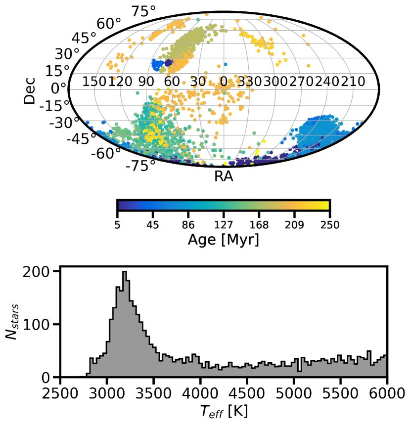
Figure 1: Top: Distribution of the selected sample across the sky and colored by the adopted age of the association (see Table 1). The all-sky coverage by TESS has unlocked new populations of stars to observe. We take advantage of this observing strategy to measure flare rates across 26 different nearby young moving groups, clusters, and associations. Bottom: Distribution of adopted effective temperatures, $T_{\textrm{eff}}$ [K] for stars in our sample. We include all stars with $T_{\textrm{eff}}\leq 6000$ K.

2.3 Flare Identification

Once we downloaded the light curves for each target, we performed the following procedure to identify stellar flares. We implemented the machine learning flare-identification methods presented and described in Feinstein et al. (2020b). This method relies on the similar time-dependent morphologies of all flare events. These flare-profiles can generally be described as a sharp rise followed by an exponential decay in the white light curve. This identification-technique implements the convolutional neural network (CNN) stella (Feinstein et al., 2020b), although other architectures have been explored for flare identification (e.g. Vida & Roettenbacher, 2018). The CNN was trained on a by-eye validated catalogue of flares from TESS Sectors 1 and 2 with 2-minute data (Günther et al., 2020).

There are several benefits to using the CNN for stellar flare identification. Primarily, the CNN is insensitive to the stellar baseline flux because it is trained to search only based on flare morphology. It is therefore relatively insensitive to the absolute flux levels, so long as the inherent noise does not overwhelm the signal itself. An additional benefit is that rotational modulation peaks — which are themselves driven by stellar heterogeneities — are not accidentally identified as flares. This holds true for stars with rotation periods, $P_{\textrm{rot}}>1$ day. This is especially advantageous for our sample of young stars, which readily exhibit rotational modulation in their light curves.

Based on these advantages, the final compiled sample of flares is unbiased towards low-amplitude/low-energy flares. It is important to note that these low-energy events are typically not identified in traditional sigma-outlier identification methods (e.g. Chang et al., 2015; Vasilyev et al., 2022). While significant developments have been achieved to better model and detrend stellar variability (e.g. Bicz et al., 2022), these methods can be computationally intensive The stella CNN models calculate the probability that a data point in a light curve is associated with a flaring event. Specifically, it takes the light curve (time, flux, flux error) as an input and returns an array with values of [0,1], which are treated as the probability a data point is (1) or is not (0) part of a flare. We ran every light curve through 10 independent stella models and averaged the outputs to ensure that our statistics were accurate. We note that in this processing, the CNN ignores 200-minutes before and after any gaps in the data. Therefore, any flares which occur during these times are not identified. From by-eye vetting of $\sim 300$ light curves, we found 2 flares within the first 200 minutes of the orbital gaps. Therefore, we estimate $\leq 120$ flares are missed in our catalog.

The stella code groups individual points with the predictions per data point when identifying a single flare event. We modified this stage of identification slightly from the original flare-identification method. Specifically, we identified all data points with a probability of being associated with a flare of $P>0.75$. Any data points that were within 4 cadences of each other were considered to be a single flare event. We did not consider any potential flares that had three or fewer points with $P>0.75$. This method rejects single-point outliers which can be assigned high probabilities of being flares. We assigned the probability of the whole flare event as the probability of the peak data point.

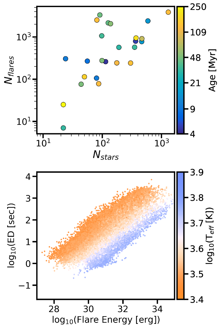
Figure 2: High level summary of the demographics of flares in our sample. Top: The number of flares identified compared to the number of stars in each nearby young moving group, cluster, or association. A linear relationship is expected. Bottom: The distribution of measured TESS energies and equivalent durations of flares in our sample, colored by the probability of the flare as identified with stella.

2.4 Modeling Flare Properties

Flares are well-described in light curves as a sudden increase in flux followed by an exponential decay. We used the analytic flare model, Llamaradas Estelares which was presented in Tovar Mendoza et al. (2022), to fit and extract parameters of flares in all of the light curves of our sample. This model builds upon the model presented in Davenport et al. (2014). Specifically, it includes the convolution of a Gaussian with a double exponential model in the flare profile.

The analytic model robustly accounts for physically-motivated flare features. Specifically, it can incorporate the flare (i) amplitude, (ii) heating timescale, (iii) rapid cooling phase timescale, and (iv) slow cooling phase timescale. We implemented a nonlinear least squares optimization to fit the flare peak time ($t_{\textrm{peak}}$), full width at half maximum (FWHM), and the amplitude ($A$) of each flare in the sample. We note that there are several other physically-motivated flare models which could be used, such as those presented in Gryciuk et al. (2017); Pietras et al. (2022); Yang et al. (2023a); these models include using two profiles to fit the impulsive and late phases of the flare. We combine the model with a second-order polynomial fit to a 1.2-hour baseline before and after the flare during only the fitting stage. This was implemented in order to account for any slope due to rotational modulation, and therefore was particularly relevant for the rapid rotators ($P_{\textrm{rot}}<2$ days).

We calculated the equivalent duration, ED, of the flare by integrating the quiescent-normalized flare flux with respect to time. We calculate the flare energy, $E_{\textrm{flare}}$, using,

$$E_{\textrm{flare}}=L_{\star}\,A\,\textrm{ED}\,s\,.$$ (1)

In Equation 1, $L_{\star}$ is the luminosity of the star and $s$ is a scaling factor defined as $s=B_{\lambda}(T_{\textrm{eff}})/B_{\lambda}(T_{\textrm{flare}})$, where $B_{\lambda}(T)$ is the Planck function. We assume that the flare temperature is 9000 K (Hawley & Fisher, 1992; Hawley et al., 1995), although recent NUV flare observations suggest this may be an underestimation (Kowalski et al., 2019; Brasseur et al., 2023; Berger et al., 2023).

2.4.1 Comparison of Flare Models

Tovar Mendoza et al. (2022) demonstrated that the flare model works well for flares with amplitudes $\geq 2$ (i.e. double the baseline flux). However, other works such as Pietras et al. (2022) have demonstrated that a double-flare profile better fits high energy flares. To quantify how well the Llamaradas Estelares model works, we refit and calculate the $\chi^{2}$ for a subset of high amplitude flares ($A\geq 0.4$) using Equation 3 in Pietras et al. (2022), a double-peak flare model, which is:

$$\begin{split}f(\tau)=\int_{0}^{\tau}\bigg{(}A_{1}\,\exp\bigg{[}\frac{-(t-B_{1})^{2}}{C_{1}^{2}}\bigg{]}\,\exp\bigg{[}\frac{(t-\tau)}{D_{1}}\bigg{]}\\ +A_{2}\,\exp\bigg{[}\frac{-(t-B_{2})^{2}}{C_{2}^{2}}\bigg{]}\,\exp\bigg{[}\frac{(t-\tau)}{D_{2}}\bigg{]}\bigg{)}\textrm{d}t\end{split}$$ (2)

where $A$ is is related to amplitude of the flare, $B$ relates to the total energy released during the flare, $C$ relates to the timescale of the flare, $D$ is related to the decay timescale, $\tau$ is the time of a given cadence, and $t$ is the time to integrate over. The subscripts 1 and 2 indicate which flare variables are associated with the first and second flare profile. We refit 900 high-amplitude flares following Equation 2. We plot the results of this refitting in Figure 3.

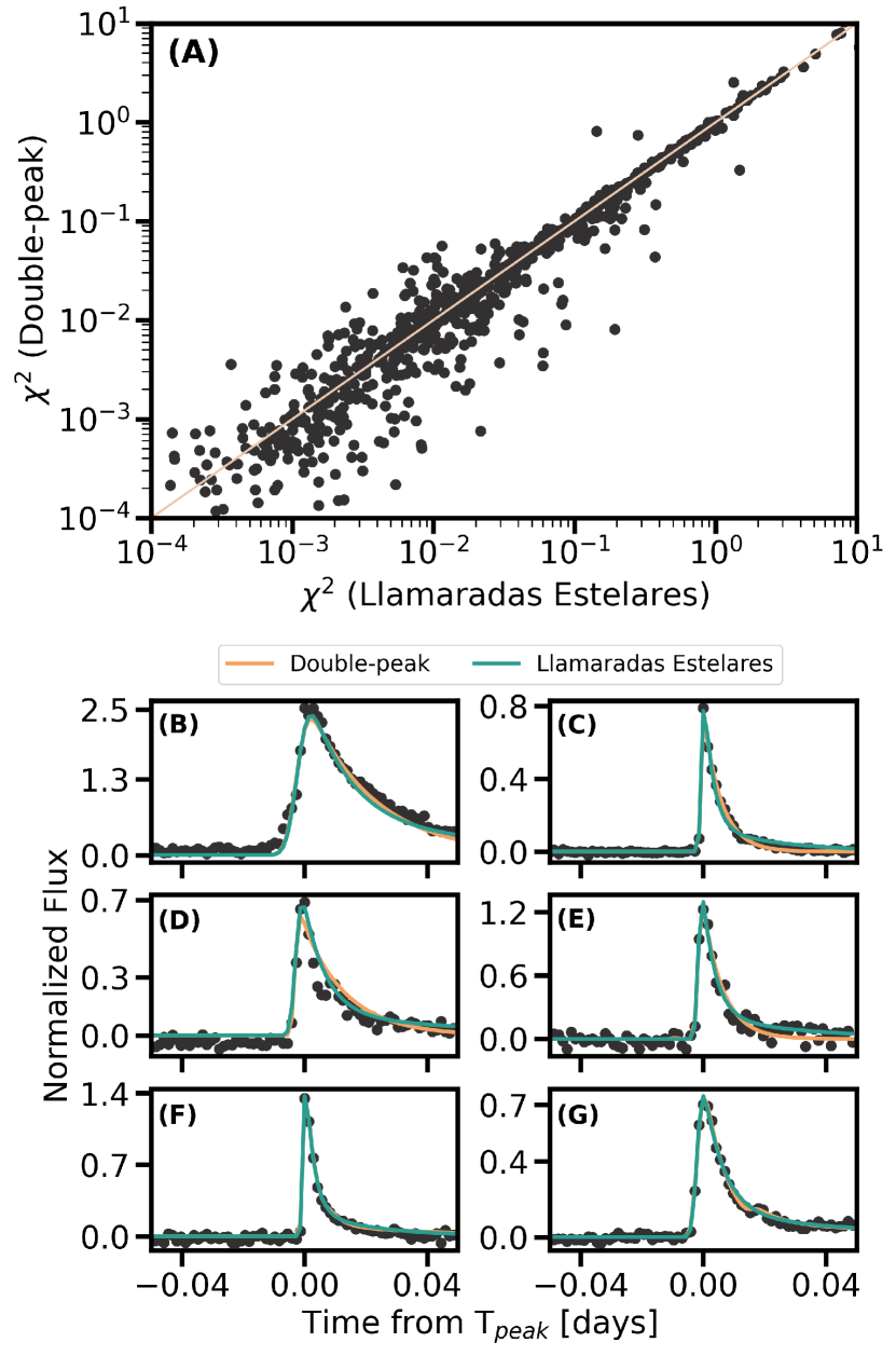
Figure 3: Comparison fits between the Llamaradas Estelares single-peak model from Tovar Mendoza et al. (2022) and the double-peak flare model from Pietras et al. (2022) for flares with $A\geq 0.4$. Top (A): Comparison in the $\chi^{2}$ between the best-fit model for 900 flares. A one-to-one line is plotted in peach to guide the eye. Across this sample of high-amplitude flares, there is good agreement between the fits for these two distinct models. Bottom: Comparison in best-fit models for a subset of flares. The best-fit Llamaradas Estelares model is plotted in blue; the best-fit double-peak model is plotted in orange. We highlight examples where the double-peak flare model has the better fit (B, C), the Llamaradas Estelares flare model has the better fit (D, E), and where the models perform equally as well (F, G). We note there is no correlation between flare amplitude and preferred model.

Broadly, we find the flare model from Tovar Mendoza et al. (2022) and Pietras et al. (2022) to fit the majority of the high-amplitude flares equally as well (Figure 3 A). We highlight several examples where one model fits better than the other in Figure 3 B-E, and cases where both profiles fit the data equally as well Figure 3 F-G. Flares which prefer the Llamaradas Estelares model tend to have a more accurately fit flare amplitude. Flares which prefer the double-peak model tend to have an extended decay timescale, which is better fit by the addition of a secondary flare. Flares which are fit equally well by both models tend to have a better fit to the amplitude in the Llamaradas Estelares model, but a better fit to the decay timescale in the double-peak flare model.

2.5 Flare Quality Checks

The stella CNNs were trained on data from TESS Sectors 1 and 2. However, the noise properties are variable across sectors in TESS data. The CNNs are therefore unable to accurately account for and capture this variation when operating on different sectors. Moreover, the original CNNs were only trained on a sample of 1,228 stars. This training sample does not necessarily encapsulate a sufficient distribution of variable stars types, such as eclipsing binaries, RR Lyraes, and fast rotators with $P_{\textrm{rot}}<1$ day (Lawson et al., 2019), which results in the CNNs not being able to properly distinguish these temporal features from flares. We therefore apply additional quality checks to ensure our flare sample has little to no contamination from other sources.

Specifically, we remove flares from our sample which did not satisfy one or more of the following criteria:

1. The amplitude of the flare must be $>0.01$, the same limits set by Feinstein et al. (2020b).

2. The flare amplitude must be at least twice the standard deviation of the light curve 30 minutes before and 45 minutes after the flare. This ensures that the feature is not a sharp noise artifact.

3. The fitted flare model parameters must be physically motivated: FWHM $>0$; $A>0$; ED $>0$.

4. The flare parameters must be $\sigma_{A}<0.5$ and $\sigma_{t_{\textrm{peak}}}<0.01$.

We find that flares are often simply mischaracterized noise when the errors on the first and fourth criteria are larger than the cut-offs. These quality checks highlight the need to continuously update machine learning models, especially when looking at data with varying instrumental systematics.

As a final check, we performed an exhaustive by-eye verification of flares from light curves for stars with flare rates, $\mathcal{R}>1$ day^-1. These stars generally tend to have $T_{\textrm{eff}}>5000$ K and TESS magnitudes $<8$. Therefore, their light curves are dominated by sharp noise which stella often mischaracterizes as flares. As a final cut, the sample only includes events that have a probability $P\geq 98\%$ of being a true flare. After performing these additional checks, we obtain a robust final flare sample of 26,355 flares originating from 3,160 stars (Figure 2).

2.6 Measuring Rotation Periods

In addition to understanding flare statistics across young stars, we measure the rotation periods, $P_{\textrm{rot}}$ of stars in our sample. We then search for correlations between $P_{\textrm{rot}}$ and Rossby number, $R_{0}$. Seligman et al. (2022) demonstrated that stars with low Rossby numbers $R_{0}<0.13$ exhibit shallower flare frequency distribution slopes. These shallower slopes are caused by an excess of high energy flares compared to lower energy flares.

In order to perform this, we describe how we measure stellar rotation periods from the TESS light curves. To this end we used michael, an open-source Python package that robustly measures $P_{\textrm{rot}}$ using a combination traditional Lomb-Scargle periodograms and wavelet transformations (Hall et al. submitted). michael measures $P_{\textrm{rot}}$ using the eleanor package, which extracts light curves from the TESS Full-Frame Images (FFIs; Feinstein et al., 2019).

We ran michael on all stars in our samples from which flares were identified. The estimated rotational periods were subsequently vetted by-eye with the michael diagnostic plots. This vetting was implemented to ensure that the measured $P_{\textrm{rot}}$ was not a harmonic of the true $P_{\textrm{rot}}$ or from an occulting companion. This led to robust measurements of rotation periods for 1,847 stars in total. Additionally, we identified 17 eclipsing binaries or potentially new planet candidates.

3 Flare Rates of Young Stars

In this section, we use the previously described methodology to estimate the flare rates of the young stars in our sample. We implement three main steps in this analysis. First, we perform the standard FFD fitting of a power-law to the distribution of flare energies described in Section 3.1. Next we fit the relationship between $R_{0}$ and flare rates in Section 3.2. Finally we fit a truncated power-law to the distribution of flare amplitudes in Section 3.3 to identify correlations between $R_{0}$ and flare distributions.

The number of stars and flares in each association varied greatly (Figure 2). This was primarily caused by the limited number of stars that had been observed at 2-minute cadence in TESS. We therefore did not measure FFD properties as a function of association. Instead, we group stars by $T_{\textrm{eff}}$ and average adopted association age.

We define the following spectral type bins by $T_{\textrm{eff}}$:

• M-stars below the fully convective boundary ($T_{\textrm{eff}}=2300-3400$ K),

• early type M-stars ($T_{\textrm{eff}}=3400-3850$ K),

• late K-stars ($T_{\textrm{eff}}=3850-4440$ K),

• early K-stars ($T_{\textrm{eff}}=4440-5270$ K),

• G-stars ($T_{\textrm{eff}}=5270-5930$ K).

We did not include any stars hotter than $T_{\textrm{eff}}>5930$ K. These hot stars generally exhibit light curves dominated by noise in the TESS observations. Additionally, we grouped stars in the following age space: $4-10$ Myr (including Upper Scorpius and TW Hydrae), $10-20$ Myr, $20-40$ Myr, $40-50$ Myr, $70-80$ Myr, $120-150$ Myr, and $150-300$ Myr. We note that there is a gap in age from $50-70$ Myr, which could be expanded with the identification of more associations in this age range.

3.1 Standard Power-Law Fits

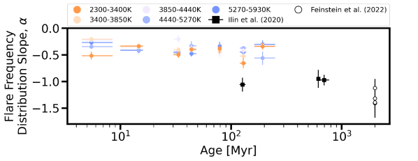
Figure 4: Measured flare-frequency distribution slopes, $\alpha$, as a function of stellar effective temperature, $T_{\textrm{eff}}$ and age. We measured these FFDs with respect to flare energy. We find the FFD slopes as a function of energy are consistent with $\alpha=-0.6~{}\textrm{to}-0.2$ for stars $<300$ Myr in TESS observations. A shallower FFD slope is indicative of more high-energy flares. We present all measured FFDs in Figure A, and all measured slopes and errors in Table 3. We find the shallowest slopes for stars $T_{\textrm{eff}}=3400-4440$ K, with a range from $\alpha=-0.44~{}\textrm{to}-0.22$. We do not include the results for stars $T_{\textrm{eff}}=3850-4440$ K and $t_{\textrm{age}}=20-40$ Myr as this bin contained only six stars with detected flares. We present the average results of measured FFD slopes for the Hyades, Pleiades, and Praesepe clusters from Ilin et al. (2021) as black squares. We present the results of measured FFD slopes for all TESS primary mission targets in white circles (Feinstein et al., 2022b) as “field-age”. We discuss what drives the difference between our sample and Ilin et al. (2021) in Section 3.1.

We fit the stars FFD slopes, approximated as a power-law, using the $T_{\textrm{eff}}$ and age bins described above. Flares were binned into 25 bins in log-space from $10^{27}-10^{35}$ erg. The FFD has a notable turnover energy, $E_{\textrm{turnover}}$, when our detection method is incomplete due the low-amplitude of those flares. The FFD slope is often fit to flares with energies $E\geq E_{\textrm{turnover}}$. We perform our fits following the same methodology. This turnover in the FFD cannot be accurately modeled with a power-law. We present our FFDs as a function of $T_{\textrm{eff}}$ and age in Figure 10; points which were fit to measure the FFD slope are presented in black, while the full FFD is presented in gray.

We fit the FFD using the MCMC method implemented in emcee (Goodman & Weare, 2010; Foreman-Mackey et al., 2013). Specifically, we fit for the slope, $\alpha$, y-intercept, $b$, and an additional noise term, $f$. This noise term accounts for an underestimation of the errors in each bin. We initialized the MCMC fit with 300 walkers and ran our fit over 5000 steps. We discarded the first 100 steps upon visual inspection, after which the steps were fully burned-in. The measured FFD slopes, $\alpha$, are presented in Figure 4. We approximate the error on the slope as the lower 16^th and upper 84^th percentiles from the MCMC fit.

Overall, we measure a shallower FFD for stars of all masses at $t_{\textrm{age}}<300$ Myr. A shallower FFD indicates there are more high-energy flares. The measured FFD slopes are shallower than those measured using smaller samples of young stars. Jackman et al. (2021) fit the three FFDs for M3-M5, M0-M2, and K5-K8 stars younger than 40 Myr that had been observed with Next Generation Transit Survey. They measured slopes of $0.94\pm 0.04$, $0.69\pm 0.05$, $0.82\pm 0.14$ per bin, which each contained $\leq 120$ flares. It is also worth noting that the slopes measured here are based on up to an order of magnitude more flares per fit. Our sample also has a longer temporal baseline, allowing for the occurrence of more high-energy flares. Accumulating more high-energy flares in the FFD, if such events occur, will result in a shallower FFD slopes. TESS flare statistics for main sequence stars have indicated steeper FFDs (Feinstein et al., 2022a). Therefore, the FFDs presented here are not strictly impacted by longer observations, but are the result of more high-energy flares on young stars.

There is a $1-3\sigma$ discrepancy between the FFD slope measured in Ilin et al. (2021) and the work presented here at ages $\sim 120$ Myr ($\alpha$ ranges from $-1.32\pm 0.19~{}\textrm{to}-0.91\pm 0.18$, depending on the $T_{\textrm{eff}}$ bin). Ilin et al. (2021) used the K2 30-minute light curves for their analysis, compared with our TESS 2-minute light curves. Additionally, our sample has $\sim 2\times$ the number of stars and $\sim 7\times$ the number of flares as in Ilin et al. (2021). First, we test if these discrepancies are driven by differences in sample binning. We reevaluate the FFDs assuming the $T_{\textrm{eff}}$ bins presented in Table 3 of Ilin et al. (2021). We find $\alpha$ remains consistent with our presented values to within $\sim 1\sigma$ of the nearest temperature bin. Second, we reevaluate the FFDs assuming the total number of flares fit in Ilin et al. (2021). We draw $n_{\textrm{fit, Ilin et al. (2021)}}$ (last column in Table 3 of Ilin et al., 2021) flares from our sample 100 times without replacement, refit the FFD, and take the average FFD slope from that sub-sample of flares to our results. We find $\alpha$ remains consistent with our presented values to $\sim 2\sigma$. We note that in most cases $n_{\textrm{fit, Ilin et al. (2021)}}<n_{\textrm{fit, this work}}$. Therefore, the increased disagreement in $\alpha$ could be due to smaller sample sizes.

Additionally, we test if the difference in $\alpha$ is driven by the cadence differences between K2 (30-minute) and TESS (2-minute). We bin all of the flares in our sample down to a 30-minute cadence, re-fit for flare $A$ and ED, and recalculate the flare energy. We re-fit the FFD for this altered sample and measure FFD slopes consistent to $\sim 1\sigma$ with those presented in this work. Therefore, the discrepancy seen here is not driven by observational differences between K2 and TESS.

Finally, we test if the differences are driven by the range of energies that are fit. The CNN-based flare detection algorithm has previously been demonstrated to be less-biased against lower energy flares. Like this work, Ilin et al. (2021) fit the FFD across flare energies which are not affected by a reduced efficiency in the low-energy flare detection, $E\geq E_{\textrm{turnover}}$. In energy space, these fits begin between $E_{f}=10^{32-33}$ erg, compared to our fits which begin between $E_{f}=10^{31-32}$ erg (Figure A). When we limit our sample to $E_{f}\geq 10^{32.5}$ erg, we find the FFD slopes become steeper and more consistent with the values of $\alpha$ presented in Ilin et al. (2021). Therefore, the difference in $\alpha$ between this work and Ilin et al. (2021) for stars with $t_{\textrm{age}}=120-150$ Myr is driven by the lower energy flares, with which we are more complete to with TESS than K2.

3.2 Flare Rate Dependence on Rossby Number

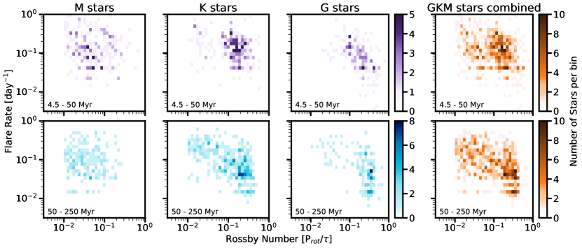
Figure 5: Comparison of Rossby Number, $R_{0}$ and flare rate for young GKM stars. For the younger sample (top row; $t_{\textrm{age}}=4.5-50$ Myr), we find no correlations between flare rate and $R_{0}$. For the slightly older sample (bottom row; $t_{\textrm{age}}=50-250$ Myr), we find no change in the average flare rate for M stars. For K and G stars, we start to see some evolution in this relationship. For K and G stars, we that as $R_{0}$ increases, the average flare rate decreases. This could indicate that as stars spin-down, their flare activity also begins to decline. We find that for the full GKM sample of stars (bottom row, rightmost column), the relationship between $R_{0}$ and flare rate is best-fit by a broken power law, with a turnover at $R_{0}=0.136$. For the younger full sample (top row, rightmost column), we find this relationship is best-fit by a single power law. The histograms are colored by number of stars in each bin.

The Rossby number, $R_{0}$, is a parameter which incorporates several properties which are known to affect the stellar dynamo, such as the rotation period and stellar mass. In the context of stellar dynamo the Rossby number indicates the dominance of the convective verses rotational dynamo. It is defined as $R_{0}=P_{\textrm{rot}}/\tau$, where $\tau$ is the convective turnover time. We convert our measured rotation periods to $R_{0}$, approximating $\tau$ following the prescription in Wright et al. (2011). We equate the flare rates, $\mathcal{R}$, for individual stars as

$$\mathcal{R}=\frac{1}{t_{\textrm{obs}}}\left(\sum_{i=1}^{N}p_{i}\right)\,.$$ (3)

In Equation (3), $\mathcal{R}$ is the flare rate in units of day^-1, $t_{\textrm{obs}}$ is the total amount of time a target was observed with TESS, and $p_{i}$ is the probability that flare $i$ is a true flare as assigned by stella. We compare the calculated $R_{0}$ to measured flare rates for all stars with measured $P_{\textrm{rot}}$. The results are presented in Figure 5.

From these results, we are able to evaluate the dependence of the flare rate on age, spectral type, and $R_{0}$. We split the sample between stars younger and older than 50 Myr. This age roughly correlates to the age at which GKM stars turn onto the main sequence. The flare rate of stars younger than 50 Myr slightly decreases with increasing $R_{0}$. However, there is a significant amount of scatter in this relationship.

As can be seen by comparing the upper and lower panels in Figure  5, the flare rate dependence on Rossby number is most evident in older, more massive stars between $50-250$ Myr. There is minimal evolution in both the average flare rate and $R_{0}$ between the two samples for M stars. For K stars, $R_{0}$ evolves more dramatically during the first 250 Myr while the scatter in the flare rate decreases. For G stars, the scatter in $R_{0}$ decreases and the average flare rate across the sample decreases. We present a compiled histogram for all stars in our sample in the right column of Figure 5.

To better understand this trend for the GKM sample, we fit three functions to the flare rate Rossby number parameter space: (i) a constant value, (ii) a single power law, and (iii) a piece-wise function consisting of a constant value and a power law. We computed the $\chi^{2}$ between each of these fits and the data. For (iii), we fit for where the $R_{0}$ turnover should occur by computing the $\chi^{2}$ across a range of $R_{0}=[0.09,0.18]$. We weighted the data points based on the density of points in a given bin (Figure 5). For $4.5-50$ Myr old stars, the distribution is best-fit with a single power law with slope $m=-0.102\pm 0.018$ and y-intercept $b=-0.660\pm 0.017$. For stars $50-250$ Myr, the distribution is best-fit with a piece-wise function of the form:

$$\mathcal{R}=\Bigg{\{}\begin{array}[]{ll}C&R_{0}\leq 0.136\\ 10^{b}*R_{0}^{m}&R_{0}>0.136\\ \end{array}$$ (4)

In Equation (4), $\mathcal{R}$ is the flare rate, $C=0.269\pm 0.007$, $m=-0.612\pm 0.039$, and $b=-1.113\pm 0.035$. The location of the turnover is consistent with what has been measured in other observations of magnetic saturation for partially and fully convective stars (e.g. $L_{X}/L_{\textrm{bol}}$; Wright et al., 2018).

With a sample of 851,168 flares detected in both Kepler 1- and 30-minute cadence data, Davenport (2016) searched for a relationship between Rossby number and relative flare luminosity. This work determined that the relationship could be fit by a broken power law, with a break at $R_{0}=0.03$ and a slope of $m\sim-1$ dominating higher $R_{0}$. However, a single power law is slightly preferred over the broken power law. While the metrics used between Davenport (2016) and this paper are different, both suggest a saturation in flares for stars with low $R_{0}$. Additionally, Medina et al. (2020) found a broken power-law relationship between $R_{0}$ and the flare rate for flares with $E_{f}>3.16\times 10^{31}$ erg, corresponding to the completeness threshold of their sample. Medina et al. (2020) analyzed light curves of 419 low-mass ($M_{\star}=0.1-0.3M_{\odot}$) main-sequence stars in the Solar neighborhood observed by TESS. They found that the flare rate saturates at $log(\mathcal{R})=-1.30\pm-0.08$ for $R_{0}<0.1$ and rapidly declines for $R_{0}>0.1$. Yang et al. (2023b) analysed 7,082 stars with measured $P_{\textrm{rot}}$ observed during TESS sectors 1–30, and found a broken-power law described the relationship between $\Delta$Flare$/L_{\star}$ for M dwarfs, with a break between $R_{0}=0.1-0.13$, which is consistent with this work. While there are differences in sample selection between our work and previous studies, all are consistent with flare rate saturation for stars with low $R_{0}$ and a steep drop-off in flare rate for stars with higher $R_{0}>0.1$.

3.3 Truncated Power-Law Fits

We search for evidence of variations of the FFDs as a function of flare amplitude versus Rossby number, $R_{0}$. This is motivated by the data presented in Seligman et al. (2022). In that work, they modeled flares driven by magnetic reconnection events driven by rotational forces as well as convective dynamo. Seligman et al. (2022) found that stars with $R_{0}<0.13$ exhibited shallower FFD slopes than stars with $R_{0}\geq 0.13$ to several sigma significance. The differences in the FFDs were indicative of relatively more high-energy flares to low-energy flares. This was interpreted as evidence of a more dominant rotational dynamo compared to the convective dynamo, which preferentially produced longer magnetic braids in the stellar coronae.

In this subsection, we test this theory with a much larger sample of stars (1,847 instead of $807$ stars). We fit the distributions separated by the fitted $R_{0}$ presented in Section 3.2. In order to perform the fits, we follow the prescription described in greater detail in Seligman et al. (2022). Here, we provide a brief summary of the prescription. Specifically, we fit a truncated power-law distribution of the form,

$$dp/dA\propto A^{-\alpha_{T}}e^{-A/A_{*}}\,.$$ (5)

In Equation (5), $A$ is the amplitude of the flare, $A_{*}$ is a flare amplitude cutoff parameter and $\alpha_{T}$ is the slope, rather than $\alpha$. We fit the slopes using the MCMC method implemented in emcee (Goodman & Weare, 2010; Foreman-Mackey et al., 2013). We used the log-likelihood function in Seligman et al. (2022) and fit for $A_{*}$ and $\alpha_{T}$. We initialized the MCMC fit with 200 walkers and evaluated the fit over 5000 steps. The first 1000 steps were discarded upon visual inspection. The results are presented in Figure 6.

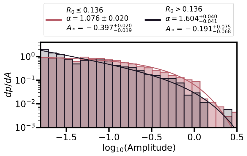
Figure 6: Flare frequency distributions, as a function of flare amplitude, for stars with $R_{0}\leq 0.12$ (red) and stars with $R_{0}>0.12$ (black). We present the best-fit model, and the best-fit values of the model slope and normalization factor in the legends. Our sample of $R_{0}\leq 0.12$ includes 13,132 flares from 800 stars; our sample of $R_{0}>0.12$ includes 5,603 flares from 747 stars. We find the stars with smaller Rossby numbers have shallower slopes, consistent with more, high-energy flares and a more dominant rotational dynamo (Seligman et al., 2022).

We find that stars with $R_{0}\leq 0.136$ have a best-fit slope of $\alpha_{T}=1.076\pm 0.020$, while stars with larger $R_{0}$ have a best-fit slope of $\alpha_{T}=1.604\pm 0.040$. This result agrees with the results presented in Seligman et al. (2022). This is not the first instance we have seen a correlation in FFDs as a function of $R_{0}$. Candelaresi et al. (2014) noted that faster rotating stars have higher superflare rates derived from Kepler data. The spectroscopic survey presented in Notsu et al. (2019) found that the maximum flare energy decreased as $P_{\textrm{rot}}$, and consequently $R_{0}$, increased. Mondrik et al. (2019) identified flares across 2,226 stars observed with MEarth and found an increase in flare rate between stars with low $R_{0}<0.04$ and stars with intermediate $R_{0}=(0.04,0.44)$, and a subsequent decrease in flare rate for stars with high $R_{0}>0.44$. While our bins of stars by $R_{0}$ are not as fine as those presented in Mondrik et al. (2019), the correlation in $\Delta R_{0}$ remains consistent.

4 Evidence for Stellar Cycles from Variable Flare Activity

The Sun undergoes an 11-year solar cycle during which it oscillates between high and low magnetic activity. This magnetic cycle manifests in a variety of observables. One of the primary indicators of the solar cycle is a stark change in the flare rate; this rate can vary by more than an order of magnitude between Solar maxima and minima (Webb & Howard, 1994). Moreover, energetics of the flares that are produced on the solar surface vary dramatically over the course of the solar cycle (Bai & Sturrock, 1987; Bai, 2003). Direct and indirect evidence of the solar cycle have also been observed in radio flux, total solar irradiance, the magnitude and geometry of the magnetic field, coronal mass ejections affiliated with flares, geomagnetic activity, cosmic ray fluxes and radioisotopes in ice cores and tree rings. For a recent review, see Hathaway (2015).

While other stars should also experience activity cycles like the Sun, they are more difficult to measure. Constraints on stellar cycles have predominantly relied on long baseline variations in stellar photometry, typically observed at cadences which cannot resolve stellar flares (see recent reviews by Jeffers et al., 2023; Işık et al., 2023). However, tracing stellar cycles via stellar flares may be more reliable, as flares are a direct consequence of magnetic activity. Scoggins et al. (2019) explored measuring the stellar cycle length of KIC 8507979, a star in the Kepler field which was observed for 18 90-day quarters. Scoggins et al. (2019) found the flare rate decreased over each quarter, which could be fit by $L_{\textrm{fl}}/L_{\textrm{Kp}}=(-9.96\pm 3.94)\times 10^{-2}\times t_{\textrm{yr}}+(2.43\pm 0.11)$, where $t_{\textrm{yr}}$ is the time in years, and $L_{\textrm{fl}}/L_{\textrm{Kp}}$ is a parameterization of the Kepler flare rate (Lurie et al., 2015).

4.1 Flare Observables from the Sun

Here, we explore observables from solar flares between 2002 and 2018 in the Reuven Ramaty High Energy Solar Spectroscopic Imager (RHESSI; Lin et al., 2002) flare catalog. The RHESSI mission observes the Sun across a wide range of X-ray energies, from 3 keV-17 MeV, with high temporal and energy resolutions as well as with high signal sensitivity. Such a wide energy range enables the ability to explore both thermal and non-thermal emission observed during flare events. Over 16 years of operations, over $100,000$ solar flares have been observed and characterized in RHESSI data. These observations covered the second half of solar Cycle 23 and the beginning of Solar Cycle 24. We use the publicly available RHESSI flare catalog to determine metrics that would be most useful when searching for evidence of stellar cycles. One potential issue with this analysis is that the HXR observations from RHESSI and white-light observations from TESS may not be directly correlated. However, there is a close spatial and temporal correspondence between HXR and white-light flares on the Sun (Fletcher et al., 2007; Krucker et al., 2011; Kleint et al., 2016). In particular, Namekata et al. (2017) demonstrated the difference spatially resolved flares as observed with RHESSI HXR and the Solar Dynamics Observatory (SDO)/Helioseismic and Magnetic Imager (HMI) white-light. In some examples, the HMI white-light emission is seen to last longer than the HXR, indicating the white-light emission is related to non-thermal electrons.

However, other examples of simultaneous HXR and white-light flare observations in (Namekata et al., 2017) show similar flare durations. Therefore, we take the HXR solar flares with energies between $25-50$ keV as likely representative of solar white-light flares, and are a comparable sample to our TESS sample. First, the total number of flares detected in the $25-50$ keV bandpass varied by 650 flares from solar maximum in 2002 to solar minimum in 2008. This variation correlates to a change in flare rate from $1.81$ to $0.02$ flares day^-1 on average. Second, the flare frequency distribution changes between solar minimum and maximum because the frequency of the highest-energy flares decreases. Finally, the total flare luminosity relative to the total luminosity correlates with the stellar cycle. This is defined by Lurie et al. (2015) as

$$\frac{L_{\textrm{flare}}}{L_{\star}}\equiv\frac{\xi_{\textrm{flare}}}{t_{\textrm{exp}}}$$ (6)

where $L_{\textrm{flare}}$ is the total luminosity emitted by flares, $L_{\star}$ is the luminosity of the star, $\xi_{\textrm{flare}}$ is sum of the equivalent duration of all flares observed, and $t_{\textrm{exp}}$ is the exposure time of the observations. These results for the Sun are presented in the left-most column of Figure 7.

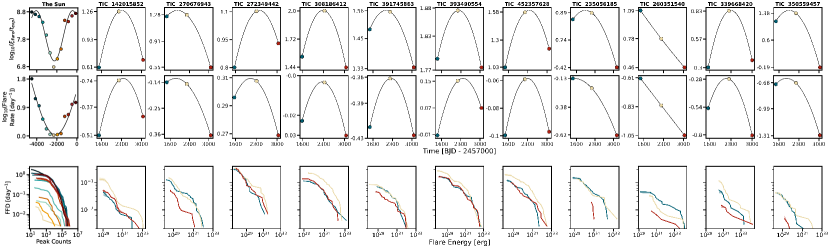
Figure 7: Comparison of three flare-driven metrics in searching for evidence of stellar cycles. Each column contains information for the Sun (left), followed by TIC 142015852, 269797536, 270676943, and 278825715. The top row shows trends in the fractional luminosity emitted in flares, $L_{fl}/L_{\textrm{TESS}}\equiv\xi_{\textrm{flare}}/t_{\textrm{exp}}$ (Lurie et al., 2015). The second and third rows show the calculated flare rate and cumulative flare frequency distribution (FFD) respectively. For the Sun, we used the RHESSI X-ray flare catalog and binned the flares per year from February 2002 - February 2014. The Sun shows clear trends in $\xi_{\textrm{flare}}/t_{\textrm{exp}}$ and flare rate over the 12-year solar cycle. The cumulative FFD shows that (i) the overall number of flares decreases, which can be seen in the flare rate as well and (ii) the high-energy flare end of the distribution decreases. A quadratic polynomial is plotted to help guide the eye. It is important to note that these fits do not provide constraints on the length of potential stellar cycles in these stars due to the limited baseline obtained with TESS thus far. We present the measured flare rates and fractional luminosity emitted for each star in Table 4

4.2 Quantifying Flare Activity over 5 Years of TESS Observations

The TESS Extended Missions have provided a five-year baseline that we can use to search for evidence of stellar cycles. This is a comparable baseline to Kepler, although with sparser sampling. We search for evidence of stellar cycles within our sample of fast rotators. Our sample contains 108 stars which have been observed for $t_{\textrm{obs}}\geq 200$ days across five years. We search for evidence of changes in the stellar magnetic activity by looking for correlations in (i) variations in the total luminosity emitted in flares (ii) the total flare rate per year and (iii) annual changes in the FFD. We group our observations by the year in which the observations were taken, even for the cases where the star was not continuously observed throughout that year (e.g. Sectors 1-26 are Year 1, Sectors 27-55 are Year 2, and Sectors 56-67 are Year 3.

We searched our 108 candidates by eye for correlations in the aforementioned criteria. The correlations are categorized into the following four options: (i) Positive: $E_{\textrm{f, max}}$ and the total number of flares has increased over five years; (ii) Negative: $E_{\textrm{f, max}}$ and the total number of flares has decreased over five years; (iii) Trough: $E_{\textrm{f, max}}$ and the total number of flares was greater in the first and third years observed with a minima in the second year; (iv) Peak: $E_{\textrm{f, max}}$ and the total number of flares was fewer in the first and third years observed with a maxima in the second year.

From these three observables, we identified eleven stars which all display evidence of scenario Peak, with the exception of one star displaying evidence of scenario Negative, which are presented in Figure 7. These stars are TIC 142015852, 235056185, 260351540, 270676943, 272349442, 308186412, 339668420, 350559457, 391745863, 393490554, and 452357628. Our sample includes seven early type M-stars, two late K-stars, one early K-star, and one G-star. TIC 272349442 is a candidate member of TW Hydrae ($t_{\textrm{age}}=10\pm 3$ Myr), TIC 142015852, 270676943, 308186412, 339668420, 350559457, and 452357628 are candidate members of Carina ($t_{\textrm{age}}=45\pm 9$ Myr), TIC 235056185 and 260351540 are candidate members of IC 2602 ($t_{\textrm{age}}=52.5\pm 2.95$ Myr), and TIC 391745863 and 393490554 are candidate members of the AB Doradus Moving Group ($t_{\textrm{age}}=133\pm 12.5$ Myr).

We report the measured $\xi_{\textrm{flare}}/t_{\textrm{exp}}$ and flare rates across all three years in presented in Figure 7 in Table 4. Across our sample, we find the largest change in flare parameters in TIC 235056185, which has a $\Delta log_{10}(\xi_{\textrm{flare}}/t_{\textrm{exp}})=1.14$ and $\Delta\mathcal{R}=0.5$. Additionally, we see some targets (e.g. TIC 350559457) become very flare quiet, going from $\mathcal{R}=0.2$ day^-1 to $\mathcal{R}=0.05$ day^-1, which is obvious when visually inspecting the light curve. For stars showing the Peak scenario, we find that the year before and after the peak do not necessarily return to the same value of $\xi_{\textrm{flare}}/t_{\textrm{exp}}$ and $\mathcal{R}$, although it does for some stars.

4.3 Flare Recovery per TESS Year

The majority of stars identified with evidence of stellar cycles exhibit the Peak scenario. To determine if this is astrophysical or driven by some unknown instrumental systematic, we perform an injection-recovery test on this sub-sample of stars. Injection-recovery tests are used to address biases in our detection method. Injection-recovery tests are typically not recommended for machine-learning detection techniques (Feinstein et al., 2020b). However, we perform them because these are some of the first results of searching for evidence of stellar cycles via flare activity.

We inject a total of 50 flares into each sector of data for our eleven stars. We draw the amplitude of our flares from a Gaussian distribution centered at a 3% increase in flux, with a standard deviation of 1%. We do not inject flares with amplitudes below 0.5%. We used the Llamaradas Estelares flare model. We fit a line between flare amplitude and FWHM from our new catalog to extract an appropriate FHWM for any given amplitude. We added additional noise to the FHWM, as the relationship between amplitude and FWHM exhibits scatter similar to distribution of flare energy and ED shown in Figure 2. Once the flares were injected, we followed the steps outlined in Sections 2.3 - 2.5 to identify these injected flares.

We considered a flare recovered if the $t_{\textrm{peak}}$ is within 15 minutes of the injected $t_{\textrm{peak}}$. We are able to recover 93% of flares with $A\geq 3$% and 80% of flares with $A<3$%. This is consistent with previous results using this flare identification method (Feinstein et al., 2020b). We note that there is a steep drop-off in flare recovery rate at $T_{\textrm{mag}}>13$, with average recovery rates dropping from 90% to 70%. The variation in recovery rates between years observed by TESS ranges from $1-8$% across all eleven targets. There is no correlation between recovery rate, $\xi_{\textrm{flare}}/t_{\textrm{exp}}$ and flare rate, with the exception of TIC 142015852 and 339668420. We find an 8% increase between Years 1 and 2, and a 3% decrease between Years 2 and 3 in the recovery rate for TIC 142015852. Additionally, we find an 1% increase between Years 1 and 2, and a 2% decrease between Years 2 and 3 in the recovery rate for TIC 339668420. An 8% change in the recovered flare rate correlates to $\Delta(\xi_{\textrm{flare}}/t_{\textrm{exp}})=0.09$, assuming ED $=1$ minute, and a $\Delta\mathcal{R}=0.03$. These estimates are smaller than the annual variations seen in flare statistics for these two stars, leading us to conclude that these variations are astrophysical.

4.4 Observing Peaks in Stellar Flare Activity

In the Section 4.3 we demonstrated that 10 out of 108 stars with $>200$ days of observations exhibited Peak behavior in their variability patterns and found no bias in flare detection as a function of year. This is approximately what we would expect to find for an unbiased sample. Our analysis requires a large number of bright flares to be observable to characterize the stellar cycle. Therefore, our sample of objects should be biased towards stars that are undergoing a local maximum, rather than a local miinimum, in their activity cycle.

It is not clear what the length of the activity cycles are for stars other than the Sun. For this order of magnitude estimate we therefore assume that the activity cycles of all stars in our sample are similar to that of the Sun. This approximation is valid if the length of stellar cycles on average is not more than an order of magnitude different than that of the sun. By observing $N\sim$108 stars for a $\tau\sim$5 year baseline, assuming that each has a $P\sim 10$ year activity cycle, we would expect that during that time period $\tau/PN\sim 50$ stars should experience a peak in their stellar cycle during the observations. Moreover, our analysis will only be sensitive to activity cycles if there is not only a peak, but also lower activity in the year before and after the peak. Therefore, the number of stars that we would expect to identify that have a peak in year 2 should be $\tau/PN/3\sim 16$. Therefore we would expect to identify $\sim 16$ stars exhibiting a peak in their activity cycle during these observations, which is similar to what we have found.

However, it is likely that there is a variety of lengths of stellar cycles in our population and the exact correspondence between the number found and the number estimated is simply a manifestation of the crude order of magnitude approximation that we employed rather than an exact correspondence. Nevertheless, this represents tentative detections of peaks in stellar activity cycles and that on average the length of these cycles is not an order of magnitude different than that of the Sun.

The results presented here are consistent with those presented in previous studies of magnetic activity cycles in young stars. Oláh et al. (2016) analyzed 29 stars from the Mount Wilson survey which had $\sim 36$ years of Ca II H & K monitoring. Roughly 16 stars in this sample have constrained ages of $<1$ Gyr via gyrochronology. This sample of stars have $P_{\textrm{rot}}=18.1\pm 12.2$ days and magnetic activity cycles of $P_{\textrm{cyc}}=7.6\pm 4.9$ years. There is significantly more dispersion in the young stellar cycle lengths than for the older stars. Oláh et al. (2016) concluded that young stars show more complex interannual variations in magnetic activity. While stars age, magnetic braking will increase the rotation of the star. Once this process has occurred, the magnetic activity cycle becomes more well-behaved, as seen on the Sun.

We apply the relationship between $log(1/P_{\textrm{rot}})$ and $log(P_{\textrm{cyc}}/P_{\textrm{rot}})$ described in Oláh et al. (2016) to estimate the activity cycles in our sample. 10 of our 11 candidates have measured $P_{\textrm{rot}}=0.41-5.22$ days. Using the best-fit slope of $0.76\pm 0.15$, we estimate the $P_{\textrm{cyc}}=0.81-1.49$ years. Strong evidence of shorter activity cycles than $\sim 3$ years may be missed by the sparse annual sampling from TESS. Redesigning the next TESS extended mission to stare at the northern and southern ecliptic poles continuously for two years, instead of alternating poles, may help resolve these shorter activity cycles, if present.

4.5 Validating Stellar Activity Cycles

The stars presented in this work present examples that stellar activity cycles could be identified by characterizing stellar flares and measuring flare rates. In addition to flare rates, it would be beneficial to conduct detailed spectroscopic follow-up of these candidates. For example, detailed monitoring of Ca II H & K lines for these targets could reveal if their activity cycles are similar to that seen from the flare rates. Unfortunately, our candidates are located too far south to have been included in the Mount Wilson HK project, which aimed to understand stellar chromospheric activity on a variety of timescales (Wilson, 1968). Monitoring of the overall XUV luminosities of these targets could provide additional insights into the variability of the targets. Additionally, more continuous time-series photometry of these targets would provide more stringent constraints on the flare variability for these targets. While long time-series photometry, such as that achieved with TESS and Kepler are ideal, more sparse but consistent photometric monitoring for stellar flares may provide useful additional supplemental data to TESS observations. This is especially true for the times when TESS is observing in the opposite ecliptic hemisphere.

The TESS Full-Frame Images (FFIs) allow for the creation of light curves for objects in $\sim 95\%$ of the sky (e.g. Feinstein et al., 2019). During its primary mission (July 2018 - July 2020), the TESS FFIs were taken every 30-minutes. During its first extended mission (July 2020 - September 2022), the FFI cadence was decreased to 10-minutes. Now, during its second extended mission (September 2022 - September 2025), the FFI cadence was again decreased to 3-minutes. At 3-minutes, we can more accurately identify and resolve the structure of stellar flares (Howard & MacGregor, 2022). A detailed search of flare variability for stars in the TESS FFIs may provide a more statistical view of how flare rates change on long timescales, and if they can yield insights into stellar activity cycles.

5 Discussion

5.1 Correlations with Far- and Near-Ultraviolet Flux

The stellar X-ray coronal emission is known to be a tracer of overall magnetic activity. Therefore, it should theoretically depend on the dynamo of the star, and on observable parameters that are related to the dynamo such as the rotational period. Empirical evidence indicates that there are distinct saturated and non-saturated regimes for coronal X-ray emission from main sequence stars. Specifically, stellar X-ray luminosity surveys have revealed that the saturation limit depends on the stellar rotation period. Namely, there is no evolution in $L_{X}/L_{\textrm{bol}}$ for stars with $P_{\textrm{rot}}<10$ days (Pizzolato et al., 2003). The rotation period is a good predictor of the X-ray luminosity for stars with longer $P_{\textrm{rot}}$.

The Far- and Near-Ultraviolet (FUV/NUV) emission is another tracer of magnetic activity. Younger, more active stars display excess luminosity in both of these wavelengths (Shkolnik, 2013). We use archival observations from the Galaxy Evolution Explorer (GALEX; Martin et al., 2005) to search for trends in FUV/NUV saturation and flare rate saturation, similar to the established X-ray trends. GALEX provides broad FUV photometry from $1350-1750\mbox{\AA}$ and NUV photometry from $1750-2750\mbox{\AA}$. We crossmatch our target stars with the GALEX catalog following the sample selection methods outline in (Schneider & Shkolnik, 2018). Specifically, we search using a $10^{\prime\prime}$ radius around the coordinates of each target in our sample. We include targets with no bad photometric flags (e.g. fuv_artifact or nuv_artifact == 0) as defined in the catalog. It is recommended by the GALEX documentation to exclude any objects with these flags associated. Additionally, we exclude targets with measured magnitudes brighter than 15, which marks the saturation limit for both the FUV and NUV photometers (Morrissey et al., 2007).Based on these thresholds, we find that 462 stars in our sample have NUV photometry and 139 stars have FUV photometry.

We investigate whether the saturation of flare rate and FUV/NUV emission are correlated with the derived $R_{0}$ in each star. We present our results comparing the FUV and NUV flux and the measured flare rate and Rossby number in Figure 8. We present the measured FUV/NUV flux normalized by the J-band flux, which acts as an activity indicator. In theory, the bolometric luminosities should be a better normalization factor than the J-band flux. However, the majority of stars in our sample do not have bolometric luminosity measurements. Therefore, we keep the normalization to $f_{J}$ while assessing FUV/NUV correlations for the larger statistical sample.

While there is tentative evidence of trends between the flare rate and the Rossby number (see Section 3.2), there is inconclusive evidence that the normalized FUV and NUV flux follow this trend. We note that the number of stars in our sample which have GALEX FUV measurements is small ($N_{\textrm{stars}}=139$) and therefore might not be representative of the broader population. It is worth noting that the NUV flux traces the photosphere for many of these stars, as opposed to the X-rays which trace coronal emission. Additionally, the FUV still has contributions from the photosphere for G stars. Therefore, it is possible that the lack of a correlation between the regimes identified for X-ray emission is due to the fact that the UV is tracing different stellar atmospheric regions that are not associated with the magnetic activity. not hold for FUV and NUV flux.

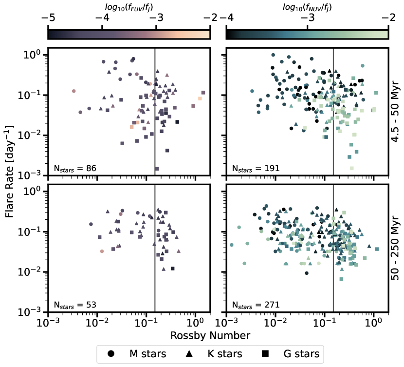
Figure 8: Calculated FUV (left) and NUV (right) GALEX flux for stars in our sample normalized by the stellar J-band flux. There is no obvious correlation between the fractional NUV/FUV flux and the measured flare rate or Rossby number. The top row shows GKM stars $<50$ Myr; the bottom row shows GKM stars $\geq 50$ Myr. M stars are shown as circles, K stars as triangles, and G stars as squares. We note that $f_{NUV}$ traces the photosphere of G, K, and massive M stars, and therefore may not be the best comparison bandpass when looking for trends in magnetic activity.

The FUV and NUV flux from GALEX is a superposition of many different emission lines. These lines trace various regions of the stellar atmosphere ranging from the corona to the photosphere depending on their formation temperatures. It is possible that the blending of lines produces the lack of correlation between FUV/NUV flux, $R_{0}$, and flare rate. Spectroscopic observations of targets with $R_{0}$ which span the transition out of the saturated regime may reveal a stronger relationship between these parameters. Pineda et al. (2021) reported evidence of broken power-law relationship between $R_{0}$ and FUV emission lines for $\sim 20$ stars observed with the Space Telescope Imaging Spectrograph on the Hubble Space Telescope. Depending on the emission line analysed, Pineda et al. (2021) found a saturated regime for $R_{0}<0.18-0.24$, with a steep drop-off for higher $R_{0}$. Additionally, Loyd et al. (2021) evaluated the relationship between FUV emission lines and $R_{0}$ for 12 Tucana-Horologium ($t_{\textrm{age}}=40$ Myr), 9 Hyades ($t_{\textrm{age}}=650$ Myr), and 7 field-aged ($t_{\textrm{age}}=2-10$ Gyr) M stars. They found a saturated $log_{10}(R_{0})=-0.876_{-0.061}^{+0.037}$, which is consistent with the X-ray flux and $R_{0}$ relationship.

The ROentgen Survey with an Imaging Telescope Array (eROSITA) instrument (Predehl et al., 2007, 2021) on the Russian Spectrum-RG mission is an all-sky X-ray survey from $\sim 0.2-8$ keV. The synergies between eROSITA and TESS are already being explored. Magaudda et al. (2022), used the measured $L_{X}$ from eROSITA and $P_{\textrm{rot}}/R_{0}$ from TESS for 704 M dwarfs to reconfirm the known X-ray activity relationship. It is possible that these combined data may show a clearer relationship between $R_{0}$ and flare rate in the X-ray than shown here in the FUV/NUV (Figure 8).

5.2 Flare Rates of Young Planet Host Stars Verses Comparison Sample

The all-sky observing strategy of TESS has revealed a new population of young transiting exoplanets. Characterization of the environment of these planets is crucial to understanding their subsequent evolution. Specifically, the stellar environment can impact how these young planets evolve into their mature counterparts.

It is unclear whether stellar flares are beneficial or detrimental to the habitability of exoplanets. It is possible that stellar flares can trigger the development of prebiotic chemistry (Rugheimer et al., 2015; Airapetian et al., 2016; Ranjan et al., 2017; Rimmer et al., 2018). On the other hand, stellar flares and affiliated coronal mass ejections can permanently alter atmospheric compositions (Chen et al., 2021). This alteration may increase the amount of atmospheric mass stripped during the early stages of planet evolution (Feinstein et al., 2020b). Therefore, understanding the environment of young transiting exoplanets can provide insight into their evolution.

To this end we compare measured flare rates of young, planet hosting stars to a statistical sample of stars with similar ages and $T_{\textrm{eff}}$ that do not have confirmed short-period planets. Specifically, we measured the flare rates of planet hosting stars with ages $<300$ Myr, comparable to the ages of our primary sample. We followed the methods outlined in Section 2 to detect and vet flares for the planet-hosting stars.

For our comparison sample, we considered stars with ages $\pm 30$ Myr of the planet hosting star and $T_{\textrm{eff}}\pm 1000$ K. For each of the stars in the control samples, we calculate the flare rate following Equation 3. We present the flare rates of planet-hosting stars and a comparable sample of stars in Figure 9 and report the measured rates in Table 2. For the control samples, we report the median flare rate, and the lower 16^th and upper 84^th percentiles.

Flare rates are slightly diminished for the majority of planet hosting stars compared to the control sample. This could be interpreted as evidence that the presence of planets inhibits magnetic reconnection events and activity, or that the presence of flares biases transit-detection algorithms. However, for all cases where the flare rates are diminished in the presence of a short-period planet, the difference between the flare rates are within 1$-\sigma$ and not statistically significant.

There are a handful of cases where stars hosting short-period planet exhibit drastically higher flare rates. The most dramatic case is for the 23 Myr AU Mic (Jeffries & Oliveira, 2005; Malo et al., 2014; Mamajek & Bell, 2014), where the flare rate is more than an order of magnitude higher than in the control sample. AU Mic and its transiting planets are generally considered as a benchmark laboratory for understanding the impact of stellar activity on young exoplanet atmospheres. The system hosts an extended debris disk (Kalas et al., 2004; Liu, 2004; Metchev et al., 2005) along with two short-period transiting planets (Plavchan et al., 2020; Martioli et al., 2021; Gilbert et al., 2022). It is worth noting that this flare rate is consistent with that measured by Gilbert et al. (2022); Feinstein et al. (2022c), and is not attributed to star-planet interactions (Ilin & Poppenhaeger, 2022). In addition to this, HIP 67522, DS Tuc A, and TOI 451 all exhibit higher flare rates than the comparison sample.

It is unclear what differentiates the planet hosting systems with higher flare rates from the control sample. France et al. (2018) and Behr et al. (2023) found that planet hosting stars are less active than an equivalent control sample of field age stars in the UV. In Figure 9 the color of the points corresponds to the effective temperature of the star. It appears that the flare rates of the planet hosting stars compared to the control sample is randomly distributed with respect to the effective temperature of the star. It is possible that there is a small age effect: the systems with higher flare rates are some of the youngest planet hosting stars: HIP 67522 is $17\pm 2$ Myr, AU Mic is $22\pm 3$ Myr, DS Tuc is $45\pm 4$ Myr and TOI 451 is $120\pm 10$ Myr. There is a slight preference for the younger systems to exhibit elevated flare rates, but this is marginal evidence at best. Future observations of these systems with elevated flare rates may reveal what causes this feature.

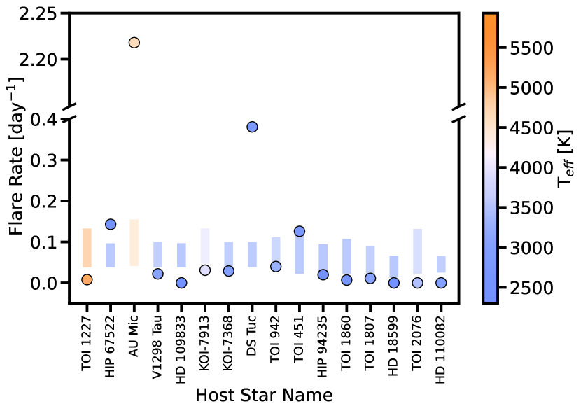
Figure 9: Comparison of flare rates from young planet host stars with respect to a comparable sample with respect to age [Myr] and $T_{\textrm{eff}}$ [K]. Circles represent the flare rate of the host star (name along the x-axis); vertical bars represent the lower 16^th and upper 84^th percentiles for the comparable sample. The majority of young planet host stars have comparable flare rates to the lower end of the comparison sample. A handful of hosts have more flares, including HIP 67522, AU Mic, DS Tuc A, and TOI 451. We find no correlation with spectral type or age which may indicate why these host stars are relatively flare quiet. The measured flare rates are presented in Table 2.

Table 2: Young Planet Host Flare Rates

Host Name	Age	Flare Rate	Comp. Sample	$N$
	[Myr]	[day-1]	Flare Rate [day-1]
TOI 1227	$11\pm 2$	0.008	$0.065_{-0.042}^{+0.074}$	168
HIP 67522	$17\pm 2$	0.169	$0.081_{-0.043}^{+0.099}$	368
AU Mic	$22\pm 3$	2.218	$0.104_{-0.066}^{+0.188}$	590
V1298 Tau	$23\pm 4$	0.022	$0.116_{-0.07}^{+0.107}$	300
HD 109833	$27\pm 3$	0.000	$0.077_{-0.039}^{+0.097}$	415
KOI-7913	$36\pm 10$	0.031	$0.152_{-0.094}^{+0.165}$	312
KOI-7368	$36\pm 10$	0.029	$0.116_{-0.071}^{+0.107}$	285
DS Tuc	$45\pm 4$	0.420	$0.104_{-0.061}^{+0.104}$	281
TOI 942	$50_{-20}^{+30}$	0.040	$0.092_{-0.049}^{+0.146}$	120
TOI 451	$120\pm 10$	0.128	$0.059_{-0.03}^{+0.136}$	204
HIP 94235	$133_{-20}^{+15}$	0.020	$0.048_{-0.028}^{+0.094}$	165
TOI 1860	$133\pm 26$	0.008	$0.049_{-0.026}^{+0.108}$	207
TOI 1807	$180\textpm 40$	0.013	$0.06_{-0.038}^{+0.11}$	53
HD 18599	$200_{-70}^{+200}$	0.000	$0.033_{-0.02}^{+0.066}$	22
TOI 2076	$204\pm 50$	0.000	$0.083_{-0.041}^{+0.122}$	55
HD 110082	$250_{-70}^{+50}$	0.000	$0.088_{-0.045}^{+0.045}$	2

Note. — $N$ is the total number of stars used to calculate the comparable sample flare rate. We highlight host stars with flare rates higher than those in the comparison sample.

6 Conclusions

In this work, we present the first measured flare rates for stars $<300$ Myr using TESS 2-minute cadence observations. We identified 26,355 flares from 3,160 stars (Figures 1 and 2). The results of our work are summarized as follows:

1. We measured the flare-frequency distribution (FFD) slope, $\alpha$, for samples of flares binned by age and $T_{\textrm{eff}}$. We find $\alpha$ saturates at $\alpha=-0.6~{}\textrm{to}-0.2$ for stars younger than 300 Myr and declines after that age (Figure 4). This is the first evidence that flare rates saturate across spectral types, as do other tracers of stellar magnetic activity,.

2. We measured rotation periods for 1,847 stars and find that the relationship between flare rate and Rossby number, $R_{0}$, is best described as a piece-wise function with a turnover at $R_{0}=0.136$ for stars $t_{\textrm{age}}>50$ Myr (Figure 5). Additionally, we find that stars with $R_{0}\leq 0.136$ have a shallower FFD than stars with $R_{0}>0.136$, which is evidence of a more dominant rotational dynamo compared to the convective dynamo (Figure 6); this is consistent with results presented in Seligman et al. (2022).

3. We searched for evidence of far- and near-Ultraviolet (FUV/NUV) flux saturation as a function of $R_{0}$, similar to what is seen in the X-ray, by cross matching our sample with the GALEX catalogs. We find no correlation between the FUV and NUV flux with flare rate (Figure 8). The NUV (and for the G-type stars, the FUV) flux traces the photosphere for many of the stars in our sample, unlike the X-ray which traces the corona. Spectrally-resolved NUV and FUV observations where the chromospheric emission lines can be isolated may be a more promising means of investigating this connection. Future synergies between eROSITA and TESS may reveal such relationships as well.

4. We compared the flare rates of planet-hosting young stars with a comparable sample with $t_{\text{age}}=t_{\textrm{age, host}}\pm 30$ Myr and $T_{\textrm{eff}}=T_{\textrm{eff, host}}\pm 1000$ K. We find that the majority of planet-hosting stars are flare inactive relative to a larger population of similar stars (although not to a statistically significant level), with the exception of HIP 67522, AU Mic, DS Tuc, and TOI 451 (Figure 9).

5. We searched for evidence of long-term stellar cycles by evaluating changes in flare rates and FFDs over five years of TESS observations. We identified ten candidates which show potential evidence of a local maxima in their stellar cycle, and one candidate which shows a decline in flare activity (Figure 7). We determine that these maxima are not due to flare-detection biases via injection recovery tests. While we are unable to obtain stellar cycle timescales from three data points, these results highlight the insights flares can bring to understanding stellar dynamos for targets with more TESS observations (e.g. stars in the continuous viewing zones) and the use of future TESS extended missions.

7 acknowledgements

We thank David Wilson for thoughtful conversations. We thank the anonymous reviewer for their insightful report, which improved the clarity and quality of this manuscript. This work made use of the open-source package, showyourwork! (Luger et al., 2021), which promotes reproducible publications. ADF acknowledges funding from NASA through the NASA Hubble Fellowship grant HST-HF2-51530.001-A awarded by STScI. DZS is supported by an NSF Astronomy and Astrophysics Postdoctoral Fellowship under award AST-2202135. This research award is partially funded by a generous gift of Charles Simonyi to the NSF Division of Astronomical Sciences. The award is made in recognition of significant contributions to Rubin Observatory’s Legacy Survey of Space and Time.

Appendix A Supplemental Material

In this appendix we present all of our best-fit slopes and intercepts for various flare-frequency distributions (FFDs) fit throughout this work. The fits outlined in Sections 3.1 are included. We present the FFDs as a function of energy in Figure 10. 100 random draws from our MCMC fitting to these distributions are shown as orange lines. We fit each distribution with $E>10^{29}$ erg, which roughly represents the turnover in each distribution. We do not fit the slope for $T_{\textrm{eff}}=[3850-4440]$ K at 20 – 40 Myr due to our limited sample size (6 stars in total).

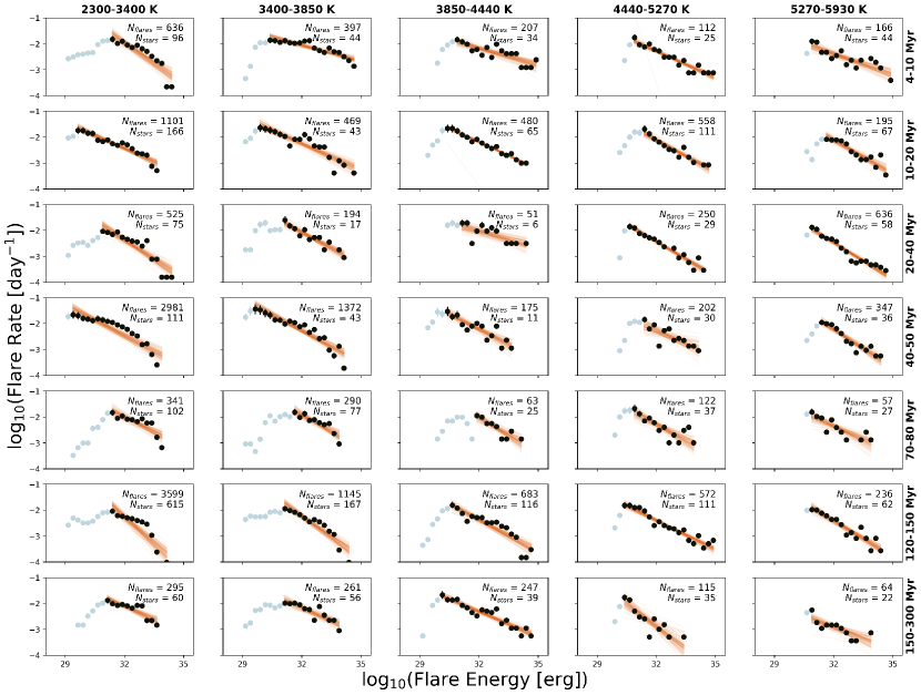
Figure 10: Flare frequency distributions (FFDs) for subgroups of stars, clustered by age and effective temperature, $T_{\textrm{eff}}$. Flares were sorted into 25 bins in log-space from $10^{27}-10^{35}$ erg. We fit the FFD from the turn-over in the binned flares, likely a result of low-energy flares missed by the flare-detection algorithm. The bins used to fit the FFD are shown in black, while all bins are shown in gray. We ran an MCMC fit to these distributions with a simple power law; 100 random samples from these fits are over-plotted in orange. We fit distributions with $>3$ bins. The best-fit slopes from these fits are presented in Figure 4.

Table 3: Best-fit slope and normalization parameters for stars of different temperatures and ages

$T_{\textrm{eff}}$ [K]	Age [Myr]	$\alpha_{\textrm{E}}$	$\sigma_{\alpha_{\textrm{E}}}$	$\beta_{\textrm{E}}$	$\sigma_{\beta_{\textrm{E}}}$	$n_{\textrm{E, fit}}$	$N_{\textrm{E}}$
2300 – 3400	4 – 10	-0.516	0.074	14.514	2.409	731	96
	10 – 20	-0.336	0.031	8.296	0.973	1183	166
	20 – 40	-0.499	0.058	13.564	1.858	526	75
	40 – 50	-0.397	0.045	10.248	1.400	3358	111
	70 – 80	-0.383	0.083	10.244	2.685	341	102
	120 – 150	-0.657	0.097	18.757	3.161	3797	615
	150 – 300	-0.341	0.063	8.799	2.029	295	60
3400 – 3850	4 – 10	-0.206	0.025	4.536	0.821	397	44
	10 – 20	-0.345	0.038	8.768	1.199	474	43
	20 – 40	-0.405	0.054	10.890	1.741	194	17
	40 – 50	-0.408	0.037	10.770	1.182	1420	43
	70 – 80	-0.432	0.075	11.893	2.471	291	77
	120 – 150	-0.525	0.062	14.557	1.998	1185	167
	150 – 300	-0.339	0.058	8.683	1.904	262	56
3850 – 4440	4 – 10	-0.221	0.040	4.884	1.314	207	34
	10 – 20	-0.350	0.016	8.998	0.545	480	65
	20 – 40	-0.202	0.077	4.425	2.492	51	6
	40 – 50	-0.379	0.062	9.873	1.982	175	11
	70 – 80	-0.455	0.102	12.498	3.347	63	25
	120 – 150	-0.419	0.046	11.010	1.494	684	116
	150 – 300	-0.323	0.029	8.026	0.929	247	39
4440 – 5270	4 – 10	-0.348	0.031	8.850	1.014	112	25
	10 – 20	-0.408	0.043	10.914	1.417	558	111
	20 – 40	-0.440	0.033	11.635	1.075	250	29
	40 – 50	-0.331	0.089	8.325	2.893	202	30
	70 – 80	-0.390	0.085	10.152	2.749	122	37
	120 – 150	-0.375	0.029	9.593	0.930	572	111
	150 – 300	-0.560	0.126	15.056	3.951	115	35
5270 – 5930	4 – 10	-0.271	0.049	6.280	1.586	166	44
	10 – 20	-0.419	0.055	11.266	1.820	195	67
	20 – 40	-0.465	0.035	12.377	1.149	636	58
	40 – 50	-0.479	0.054	13.071	1.780	347	36
	70 – 80	-0.337	0.083	8.416	2.656	57	27
	120 – 150	-0.450	0.045	11.977	1.460	236	62
	150 – 300	-0.305	0.081	6.826	2.598	64	22

Note. — $n_{\textrm{E, fit}}$ is the number of flares fit per bin; $N_{E}$ is the number of stars in each bin.

Table 4: Evidence of stellar cycles from variable flare properties

TIC		log${}_{10}(\xi_{\textrm{flare}}/t_{\textrm{exp}})$			$\mathcal{R}$ [d-1]
	Year 1	Year 2	Year 3	Year 1	Year 2	Year 3
142015852	0.61	1.26	0.69	0.31	0.58	0.38
270676943	1.26	1.28	0.55	0.72	0.71	0.43
272349442	0.80	1.10	0.93	1.98	2.03	1.86
308186412	1.54	2.00	1.43	0.95	0.99	0.93
391745863	1.49	1.56	1.33	0.38	0.44	0.37
393490554	1.79	1.88	1.77	0.97	1.42	1.17
452357628	1.03	1.58	1.21	0.80	0.87	0.80
235056185	0.73	0.89	-0.41	0.74	0.61	0.24
260351540	1.09	0.78	0.46	0.24	0.15	0.09
339668420	0.30	0.83	0.37	0.28	0.53	0.16
350559457	1.15	1.38	-0.19	0.20	0.21	0.05

TESS

References

- Abadi et al. (2016) Abadi, M., Agarwal, A., Barham, P., et al. 2016, ArXiv e-prints. https://arxiv.org/abs/1603.04467
- Airapetian et al. (2016) Airapetian, V. S., Glocer, A., Gronoff, G., Hébrard, E., & Danchi, W. 2016, Nature Geoscience, 9, 452, doi: 10.1038/ngeo2719
- Argiroffi et al. (2019) Argiroffi, C., Reale, F., Drake, J. J., et al. 2019, Nature Astronomy, 3, 742, doi: 10.1038/s41550-019-0781-4
- Astropy Collaboration et al. (2013) Astropy Collaboration, Robitaille, T. P., Tollerud, E. J., et al. 2013, A&A, 558, A33, doi: 10.1051/0004-6361/201322068
- Bai (2003) Bai, T. 2003, ApJ, 591, 406, doi: 10.1086/375295
- Bai & Sturrock (1987) Bai, T., & Sturrock, P. A. 1987, Nature, 327, 601, doi: 10.1038/327601a0
- Baum et al. (2022) Baum, A. C., Wright, J. T., Luhn, J. K., & Isaacson, H. 2022, AJ, 163, 183, doi: 10.3847/1538-3881/ac5683
- Behr et al. (2023) Behr, P. R., France, K., Brown, A., et al. 2023, AJ, 166, 35, doi: 10.3847/1538-3881/acdb70
- Bell et al. (2015) Bell, C. P. M., Mamajek, E. E., & Naylor, T. 2015, MNRAS, 454, 593, doi: 10.1093/mnras/stv1981
- Benz & Güdel (2010) Benz, A. O., & Güdel, M. 2010, ARA&A, 48, 241, doi: 10.1146/annurev-astro-082708-101757
- Berdyugina (2005) Berdyugina, S. V. 2005, Living Reviews in Solar Physics, 2, 8, doi: 10.12942/lrsp-2005-8
- Berger et al. (2023) Berger, V. L., Hinkle, J. T., Tucker, M. A., et al. 2023, arXiv e-prints, arXiv:2312.12511, doi: 10.48550/arXiv.2312.12511
- Bicz et al. (2022) Bicz, K., Falewicz, R., Pietras, M., Siarkowski, M., & Preś, P. 2022, ApJ, 935, 102, doi: 10.3847/1538-4357/ac7ab3
- Borucki et al. (2010) Borucki, W. J., Koch, D., Basri, G., et al. 2010, Science, 327, 977, doi: 10.1126/science.1185402
- Brasseur et al. (2023) Brasseur, C. E., Osten, R. A., Tristan, I. I., & Kowalski, A. F. 2023, ApJ, 944, 5, doi: 10.3847/1538-4357/acab59
- Candelaresi et al. (2014) Candelaresi, S., Hillier, A., Maehara, H., Brand enburg, A., & Shibata, K. 2014, ApJ, 792, 67, doi: 10.1088/0004-637X/792/1/67
- Carrington (1859) Carrington, R. C. 1859, MNRAS, 20, 13, doi: 10.1093/mnras/20.1.13
- Chang et al. (2015) Chang, S. W., Byun, Y. I., & Hartman, J. D. 2015, ApJ, 814, 35, doi: 10.1088/0004-637X/814/1/35
- Chen et al. (2021) Chen, H., Zhan, Z., Youngblood, A., et al. 2021, Nature Astronomy, 5, 298, doi: 10.1038/s41550-020-01264-1
- Clette et al. (2014) Clette, F., Svalgaard, L., Vaquero, J. M., & Cliver, E. W. 2014, Space Sci. Rev., 186, 35, doi: 10.1007/s11214-014-0074-2
- Crosby et al. (1993) Crosby, N. B., Aschwanden, M. J., & Dennis, B. R. 1993, Sol. Phys., 143, 275, doi: 10.1007/BF00646488
- Curtis et al. (2019) Curtis, J. L., Agüeros, M. A., Mamajek, E. E., Wright, J. T., & Cummings, J. D. 2019, AJ, 158, 77, doi: 10.3847/1538-3881/ab2899
- Davenport (2016) Davenport, J. R. A. 2016, ApJ, 829, 23, doi: 10.3847/0004-637X/829/1/23
- Davenport et al. (2019) Davenport, J. R. A., Covey, K. R., Clarke, R. W., et al. 2019, ApJ, 871, 241, doi: 10.3847/1538-4357/aafb76
- Davenport et al. (2020) Davenport, J. R. A., Mendoza, G. T., & Hawley, S. L. 2020, AJ, 160, 36, doi: 10.3847/1538-3881/ab9536
- Davenport et al. (2014) Davenport, J. R. A., Hawley, S. L., Hebb, L., et al. 2014, ApJ, 797, 122, doi: 10.1088/0004-637X/797/2/122
- Doyle et al. (2020) Doyle, L., Ramsay, G., & Doyle, J. G. 2020, arXiv e-prints, arXiv:2003.14410. https://arxiv.org/abs/2003.14410
- Feigelson & Montmerle (1999) Feigelson, E. D., & Montmerle, T. 1999, ARA&A, 37, 363, doi: 10.1146/annurev.astro.37.1.363
- Feinstein et al. (2020a) Feinstein, A., Montet, B., & Ansdell, M. 2020a, The Journal of Open Source Software, 5, 2347, doi: 10.21105/joss.02347
- Feinstein et al. (2020b) Feinstein, A. D., Montet, B. T., Ansdell, M., et al. 2020b, AJ, 160, 219, doi: 10.3847/1538-3881/abac0a
- Feinstein et al. (2022a) Feinstein, A. D., Seligman, D. Z., Günther, M. N., & Adams, F. C. 2022a, ApJ, 925, L9, doi: 10.3847/2041-8213/ac4b5e
- Feinstein et al. (2022b) —. 2022b, ApJ, 925, L9, doi: 10.3847/2041-8213/ac4b5e
- Feinstein et al. (2019) Feinstein, A. D., Montet, B. T., Foreman-Mackey, D., et al. 2019, PASP, 131, 094502, doi: 10.1088/1538-3873/ab291c
- Feinstein et al. (2022c) Feinstein, A. D., France, K., Youngblood, A., et al. 2022c, AJ, 164, 110, doi: 10.3847/1538-3881/ac8107
- Fletcher et al. (2007) Fletcher, L., Hannah, I. G., Hudson, H. S., & Metcalf, T. R. 2007, ApJ, 656, 1187, doi: 10.1086/510446
- Fletcher et al. (2011) Fletcher, L., Dennis, B. R., Hudson, H. S., et al. 2011, Space Sci. Rev., 159, 19, doi: 10.1007/s11214-010-9701-8
- Foreman-Mackey et al. (2013) Foreman-Mackey, D., Hogg, D. W., Lang, D., & Goodman, J. 2013, PASP, 125, 306, doi: 10.1086/670067
- France et al. (2018) France, K., Arulanantham, N., Fossati, L., et al. 2018, ApJS, 239, 16, doi: 10.3847/1538-4365/aae1a3
- France et al. (2016) France, K., Loyd, R. O. P., Youngblood, A., et al. 2016, ApJ, 820, 89, doi: 10.3847/0004-637X/820/2/89
- Gagné et al. (2018a) Gagné, J., Fontaine, G., Simon, A., & Faherty, J. K. 2018a, ApJ, 861, L13, doi: 10.3847/2041-8213/aacdff
- Gagné et al. (2018b) Gagné, J., Mamajek, E. E., Malo, L., et al. 2018b, ApJ, 856, 23, doi: 10.3847/1538-4357/aaae09
- Gaia Collaboration et al. (2016) Gaia Collaboration, Prusti, T., de Bruijne, J. H. J., et al. 2016, A&A, 595, A1, doi: 10.1051/0004-6361/201629272
- Gaia Collaboration et al. (2018) Gaia Collaboration, Brown, A. G. A., Vallenari, A., et al. 2018, A&A, 616, A1, doi: 10.1051/0004-6361/201833051
- Galindo-Guil et al. (2022) Galindo-Guil, F. J., Barrado, D., Bouy, H., et al. 2022, A&A, 664, A70, doi: 10.1051/0004-6361/202141114
- Gilbert et al. (2022) Gilbert, E. A., Barclay, T., Quintana, E. V., et al. 2022, AJ, 163, 147, doi: 10.3847/1538-3881/ac23ca
- Ginsburg et al. (2019) Ginsburg, A., Sipőcz, B. M., Brasseur, C. E., et al. 2019, AJ, 157, 98, doi: 10.3847/1538-3881/aafc33
- Goodman & Weare (2010) Goodman, J., & Weare, J. 2010, Communications in Applied Mathematics and Computational Science, 5, 65, doi: 10.2140/camcos.2010.5.65
- Gryciuk et al. (2017) Gryciuk, M., Siarkowski, M., Sylwester, J., et al. 2017, Sol. Phys., 292, 77, doi: 10.1007/s11207-017-1101-8
- Günther et al. (2020) Günther, M. N., Zhan, Z., Seager, S., et al. 2020, AJ, 159, 60, doi: 10.3847/1538-3881/ab5d3a
- Hathaway (2015) Hathaway, D. H. 2015, Living Reviews in Solar Physics, 12, 4, doi: 10.1007/lrsp-2015-4
- Hawley et al. (2014) Hawley, S. L., Davenport, J. R. A., Kowalski, A. F., et al. 2014, ApJ, 797, 121, doi: 10.1088/0004-637X/797/2/121
- Hawley & Fisher (1992) Hawley, S. L., & Fisher, G. H. 1992, ApJS, 78, 565, doi: 10.1086/191640
- Hawley et al. (1995) Hawley, S. L., Fisher, G. H., Simon, T., et al. 1995, ApJ, 453, 464, doi: 10.1086/176408
- Hilton et al. (2010) Hilton, E. J., West, A. A., Hawley, S. L., & Kowalski, A. F. 2010, AJ, 140, 1402, doi: 10.1088/0004-6256/140/5/1402
- Howard & MacGregor (2022) Howard, W. S., & MacGregor, M. A. 2022, ApJ, 926, 204, doi: 10.3847/1538-4357/ac426e
- Hunter et al. (2007) Hunter, J. D., et al. 2007, Computing in science and engineering, 9, 90
- Işık et al. (2023) Işık, E., van Saders, J. L., Reiners, A., & Metcalfe, T. S. 2023, Space Sci. Rev., 219, 70, doi: 10.1007/s11214-023-01016-3
- Ilin & Poppenhaeger (2022) Ilin, E., & Poppenhaeger, K. 2022, MNRAS, 513, 4579, doi: 10.1093/mnras/stac1232
- Ilin et al. (2019) Ilin, E., Schmidt, S. J., Davenport, J. R. A., & Strassmeier, K. G. 2019, A&A, 622, A133, doi: 10.1051/0004-6361/201834400
- Ilin et al. (2021) Ilin, E., Schmidt, S. J., Poppenhäger, K., et al. 2021, A&A, 645, A42, doi: 10.1051/0004-6361/202039198
- Jackman et al. (2021) Jackman, J. A. G., Wheatley, P. J., Acton, J. S., et al. 2021, MNRAS, 504, 3246, doi: 10.1093/mnras/stab979
- Jeffers et al. (2023) Jeffers, S. V., Kiefer, R., & Metcalfe, T. S. 2023, Space Sci. Rev., 219, 54, doi: 10.1007/s11214-023-01000-x
- Jeffries & Oliveira (2005) Jeffries, R. D., & Oliveira, J. M. 2005, MNRAS, 358, 13, doi: 10.1111/j.1365-2966.2005.08820.x
- Jenkins et al. (2016) Jenkins, J. M., Twicken, J. D., McCauliff, S., et al. 2016, in Society of Photo-Optical Instrumentation Engineers (SPIE) Conference Series, Vol. 9913, Software and Cyberinfrastructure for Astronomy IV, 99133E, doi: 10.1117/12.2233418
- Kalas et al. (2004) Kalas, P., Liu, M. C., & Matthews, B. C. 2004, Science, 303, 1990, doi: 10.1126/science.1093420
- Kerr et al. (2021) Kerr, R. M. P., Rizzuto, A. C., Kraus, A. L., & Offner, S. S. R. 2021, ApJ, 917, 23, doi: 10.3847/1538-4357/ac0251
- Kilcik et al. (2014) Kilcik, A., Yurchyshyn, V. B., Ozguc, A., & Rozelot, J. P. 2014, ApJ, 794, L2, doi: 10.1088/2041-8205/794/1/L2
- Kleint et al. (2016) Kleint, L., Heinzel, P., Judge, P., & Krucker, S. 2016, ApJ, 816, 88, doi: 10.3847/0004-637X/816/2/88
- Kounkel et al. (2020) Kounkel, M., Covey, K., & Stassun, K. G. 2020, AJ, 160, 279, doi: 10.3847/1538-3881/abc0e6
- Kowalski et al. (2009) Kowalski, A. F., Hawley, S. L., Hilton, E. J., et al. 2009, AJ, 138, 633, doi: 10.1088/0004-6256/138/2/633
- Kowalski et al. (2010) Kowalski, A. F., Hawley, S. L., Holtzman, J. A., Wisniewski, J. P., & Hilton, E. J. 2010, ApJ, 714, L98, doi: 10.1088/2041-8205/714/1/L98
- Kowalski et al. (2013) Kowalski, A. F., Hawley, S. L., Wisniewski, J. P., et al. 2013, ApJS, 207, 15, doi: 10.1088/0067-0049/207/1/15
- Kowalski et al. (2019) Kowalski, A. F., Wisniewski, J. P., Hawley, S. L., et al. 2019, ApJ, 871, 167, doi: 10.3847/1538-4357/aaf058
- Krucker et al. (2011) Krucker, S., Hudson, H. S., Jeffrey, N. L. S., et al. 2011, ApJ, 739, 96, doi: 10.1088/0004-637X/739/2/96
- Lawson et al. (2019) Lawson, K. D., Wisniewski, J. P., Bellm, E. C., Kowalski, A. F., & Shupe, D. L. 2019, AJ, 158, 119, doi: 10.3847/1538-3881/ab3461
- Lean (1987) Lean, J. 1987, J. Geophys. Res., 92, 839, doi: 10.1029/JD092iD01p00839
- Lehtinen et al. (2016) Lehtinen, J., Jetsu, L., Hackman, T., Kajatkari, P., & Henry, G. W. 2016, A&A, 588, A38, doi: 10.1051/0004-6361/201527420
- Lin et al. (2023) Lin, J., Wang, F., Deng, L., et al. 2023, ApJ, 958, 1, doi: 10.3847/1538-4357/ad0469
- Lin et al. (2002) Lin, R. P., Dennis, B. R., Hurford, G. J., et al. 2002, Sol. Phys., 210, 3, doi: 10.1023/A:1022428818870
- Liu (2004) Liu, M. C. 2004, Science, 305, 1442, doi: 10.1126/science.1102929
- Loyd et al. (2021) Loyd, R. O. P., Shkolnik, E. L., Schneider, A. C., et al. 2021, ApJ, 907, 91, doi: 10.3847/1538-4357/abd0f0
- Lu & Hamilton (1991) Lu, E. T., & Hamilton, R. J. 1991, ApJ, 380, L89, doi: 10.1086/186180
- Luger et al. (2021) Luger, R., Bedell, M., Foreman-Mackey, D., et al. 2021, arXiv e-prints, arXiv:2110.06271. https://arxiv.org/abs/2110.06271
- Luhman (2007) Luhman, K. L. 2007, ApJS, 173, 104, doi: 10.1086/520114
- Lurie et al. (2015) Lurie, J. C., Davenport, J. R. A., Hawley, S. L., et al. 2015, ApJ, 800, 95, doi: 10.1088/0004-637X/800/2/95
- Maehara et al. (2015) Maehara, H., Shibayama, T., Notsu, Y., et al. 2015, Earth, Planets and Space, 67, 59, doi: 10.1186/s40623-015-0217-z
- Magaudda et al. (2022) Magaudda, E., Stelzer, B., Raetz, S., et al. 2022, A&A, 661, A29, doi: 10.1051/0004-6361/202141617
- Malo et al. (2014) Malo, L., Doyon, R., Feiden, G. A., et al. 2014, ApJ, 792, 37. https://arxiv.org/abs/1406.6750
- Mamajek & Bell (2014) Mamajek, E. E., & Bell, C. P. M. 2014, MNRAS, 445, 2169, doi: 10.1093/mnras/stu1894
- Martin et al. (2005) Martin, D. C., Fanson, J., Schiminovich, D., et al. 2005, ApJ, 619, L1, doi: 10.1086/426387
- Martioli et al. (2021) Martioli, E., Hébrard, G., Correia, A. C. M., Laskar, J., & Lecavelier des Etangs, A. 2021, A&A, 649, A177, doi: 10.1051/0004-6361/202040235
- Medina et al. (2020) Medina, A. A., Winters, J. G., Irwin, J. M., & Charbonneau, D. 2020, ApJ, 905, 107, doi: 10.3847/1538-4357/abc686
- Metchev et al. (2005) Metchev, S. A., Eisner, J. A., Hillenbrand, L. A., & Wolf, S. 2005, ApJ, 622, 451, doi: 10.1086/427869
- Mondrik et al. (2019) Mondrik, N., Newton, E., Charbonneau, D., & Irwin, J. 2019, ApJ, 870, 10, doi: 10.3847/1538-4357/aaee64
- Morrissey et al. (2007) Morrissey, P., Conrow, T., Barlow, T. A., et al. 2007, ApJS, 173, 682, doi: 10.1086/520512
- Murphy & Lawson (2015) Murphy, S. J., & Lawson, W. A. 2015, MNRAS, 447, 1267, doi: 10.1093/mnras/stu2450
- Namekata et al. (2017) Namekata, K., Sakaue, T., Watanabe, K., et al. 2017, ApJ, 851, 91, doi: 10.3847/1538-4357/aa9b34
- Notsu et al. (2013) Notsu, Y., Shibayama, T., Maehara, H., et al. 2013, ApJ, 771, 127, doi: 10.1088/0004-637X/771/2/127
- Notsu et al. (2019) Notsu, Y., Maehara, H., Honda, S., et al. 2019, ApJ, 876, 58, doi: 10.3847/1538-4357/ab14e6
- Okamoto et al. (2021) Okamoto, S., Notsu, Y., Maehara, H., et al. 2021, ApJ, 906, 72, doi: 10.3847/1538-4357/abc8f5
- Oláh et al. (2016) Oláh, K., Kővári, Z., Petrovay, K., et al. 2016, A&A, 590, A133, doi: 10.1051/0004-6361/201628479
- Orrall & Zirker (1976) Orrall, F. Q., & Zirker, J. B. 1976, ApJ, 208, 618, doi: 10.1086/154642
- Osten et al. (2005) Osten, R. A., Hawley, S. L., Allred, J. C., Johns-Krull, C. M., & Roark, C. 2005, ApJ, 621, 398, doi: 10.1086/427275
- Paudel et al. (2018) Paudel, R. R., Gizis, J. E., Mullan, D. J., et al. 2018, ApJ, 858, 55, doi: 10.3847/1538-4357/aab8fe
- Pecaut & Mamajek (2016) Pecaut, M. J., & Mamajek, E. E. 2016, MNRAS, 461, 794, doi: 10.1093/mnras/stw1300
- Pietras et al. (2022) Pietras, M., Falewicz, R., Siarkowski, M., Bicz, K., & Preś, P. 2022, ApJ, 935, 143, doi: 10.3847/1538-4357/ac8352
- Pineda et al. (2021) Pineda, J. S., Youngblood, A., & France, K. 2021, ApJ, 911, 111, doi: 10.3847/1538-4357/abe8d7
- Pizzolato et al. (2003) Pizzolato, N., Maggio, A., Micela, G., Sciortino, S., & Ventura, P. 2003, A&A, 397, 147, doi: 10.1051/0004-6361:20021560
- Plavchan et al. (2020) Plavchan, P., Barclay, T., Gagné, J., et al. 2020, Nature, 582, 497, doi: 10.1038/s41586-020-2400-z
- Predehl et al. (2007) Predehl, P., Andritschke, R., Bornemann, W., et al. 2007, in Society of Photo-Optical Instrumentation Engineers (SPIE) Conference Series, Vol. 6686, UV, X-Ray, and Gamma-Ray Space Instrumentation for Astronomy XV, ed. O. H. Siegmund, 668617, doi: 10.1117/12.733583
- Predehl et al. (2021) Predehl, P., Andritschke, R., Arefiev, V., et al. 2021, A&A, 647, A1, doi: 10.1051/0004-6361/202039313
- Price-Whelan et al. (2018) Price-Whelan, A. M., Sipőcz, B. M., Günther, H. M., et al. 2018, AJ, 156, 123, doi: 10.3847/1538-3881/aabc4f
- Ranjan et al. (2017) Ranjan, S., Wordsworth, R., & Sasselov, D. D. 2017, ApJ, 843, 110, doi: 10.3847/1538-4357/aa773e
- Ricker et al. (2015) Ricker, G. R., Winn, J. N., Vanderspek, R., et al. 2015, Journal of Astronomical Telescopes, Instruments, and Systems, 1, 014003, doi: 10.1117/1.JATIS.1.1.014003
- Rimmer et al. (2018) Rimmer, P. B., Xu, J., Thompson, S. J., et al. 2018, Science Advances, 4, eaar3302, doi: 10.1126/sciadv.aar3302
- Röser et al. (2016) Röser, S., Schilbach, E., & Goldman, B. 2016, A&A, 595, A22, doi: 10.1051/0004-6361/201629158
- Rugheimer et al. (2015) Rugheimer, S., Segura, A., Kaltenegger, L., & Sasselov, D. 2015, ApJ, 806, 137, doi: 10.1088/0004-637X/806/1/137
- Saar & Brandenburg (1999) Saar, S. H., & Brandenburg, A. 1999, ApJ, 524, 295, doi: 10.1086/307794
- Schmitt et al. (2019) Schmitt, J. H. M. M., Ioannidis, P., Robrade, J., Czesla, S., & Schneider, P. C. 2019, A&A, 628, A79, doi: 10.1051/0004-6361/201935374
- Schneider & Shkolnik (2018) Schneider, A. C., & Shkolnik, E. L. 2018, AJ, 155, 122, doi: 10.3847/1538-3881/aaaa24
- Scoggins et al. (2019) Scoggins, M. T., Davenport, J. R. A., & Covey, K. R. 2019, Research Notes of the American Astronomical Society, 3, 137, doi: 10.3847/2515-5172/ab45a0
- Seligman et al. (2022) Seligman, D. Z., Rogers, L. A., Feinstein, A. D., et al. 2022, ApJ, 929, 54, doi: 10.3847/1538-4357/ac5b69
- Shibayama et al. (2013) Shibayama, T., Maehara, H., Notsu, S., et al. 2013, ApJS, 209, 5, doi: 10.1088/0067-0049/209/1/5
- Shkolnik (2013) Shkolnik, E. L. 2013, ApJ, 766, 9, doi: 10.1088/0004-637X/766/1/9
- Silverberg et al. (2016) Silverberg, S. M., Kowalski, A. F., Davenport, J. R. A., et al. 2016, ApJ, 829, 129, doi: 10.3847/0004-637X/829/2/129
- Smith et al. (2005) Smith, K., Güdel, M., & Audard, M. 2005, A&A, 436, 241, doi: 10.1051/0004-6361:20042054
- Tarricq et al. (2021) Tarricq, Y., Soubiran, C., Casamiquela, L., et al. 2021, A&A, 647, A19, doi: 10.1051/0004-6361/202039388
- Tofflemire et al. (2021) Tofflemire, B. M., Rizzuto, A. C., Newton, E. R., et al. 2021, AJ, 161, 171, doi: 10.3847/1538-3881/abdf53