Subleading analysis for $S^{3}$ partition functions of $\mathcal{N}=2$ holographic SCFTs

Abstract

We investigate the 3-sphere partition functions of various 3d $\mathcal{N}=2$ holographic SCFTs arising from the $N$ stack of M2-branes in the ’t Hooft limit both analytically and numerically. We first employ a saddle point approximation to evaluate the free energy $F=-\log Z$ at the planar level, tracking the first subleading corrections in the large ’t Hooft coupling $\lambda$ expansion. Subsequently, we improve these results by determining the planar free energy to all orders in the large $\lambda$ expansion via numerical analysis. Remarkably, the resulting planar free energies turn out to take a universal form, supporting a prediction that these $S^{3}$ partition functions are all given in terms of an Airy function even beyond the special cases where the Airy formulae were derived analytically in the literature; in this context we also present new Airy conjectures in several examples. The subleading behaviors we captured encode a part of quantum corrections to the M-theory path integrals around dual asymptotically Euclidean AdS₄ backgrounds with the corresponding internal manifolds through holographic duality.

1 Introduction

The AdS/CFT correspondence Maldacena:1997re ; Witten:1998qj has provided a novel way to explore string or M-theory path integrals around asymptotically Euclidean AdS backgrounds in terms of dual CFT partition functions on the conformal boundaries, thereby shedding light on the quantum nature of gravity. A conventional perturbative analysis for CFT partition functions valid in the weak coupling regime could not be directly employed to comprehend the perturbative expansion of corresponding string/M-theory path integrals, however, since the AdS/CFT correspondence is featured as a strong-weak duality.

Supersymmetric localization Pestun:2007rz has enabled our community to overcome this technical obstacle by providing finite-dimensional matrix models that capture various supersymmetric partition functions exactly, even in the strong coupling regime. In particular, various supersymmetric partition functions of holographic superconformal field theories (SCFT) have been extensively analyzed based on their matrix model representations as a means to unravel string/M-theory path integrals around dual supersymmetric asymptotically Euclidean AdS backgrounds.

Of particular interest in this line of research is the supersymmetric partition function on the round 3-sphere, whose corresponding free energy $F=-\log Z_{S^{3}}$ is regarded as a good measure for the degrees of freedom in a given theory Jafferis:2011zi ; Casini:2011kv ; Casini:2012ei . Following the pioneering work of Kapustin:2009kz , the $S^{3}$ partition function has been written in terms of a matrix model for general $\mathcal{N}\geq 2$ Chern-Simons-matter theories employing supersymmetric localization Kapustin:2010xq ; Herzog:2010hf ; Santamaria:2010dm ; Jafferis:2010un ; Martelli:2011qj ; Cheon:2011vi ; Jafferis:2011zi . For the $S^{3}$ partition function of $\mathcal{N}=2$ holographic SCFTs, in particular, the corresponding matrix models have been evaluated and compared with holographic dual quantities in a specific regime of parameters describing the theory. The first example was observed in a duality between M-theory on AdS${}_{4}\times S^{7}/\mathbb{Z}_{k}$ and the U$(N)_{k}\times$U$(N)_{-k}$ ABJM theory arising from the $N$ stack of M2 branes probing the orbifold singularity of the cone over $S_{7}/\mathbb{Z}_{k}$ Aharony:2008ug ; in this example, the gravitational free energy of the M-theory captured by the classical on-shell action in the semi-classical limit was successfully matched with the ABJM $S^{3}$ free energy in the ’t Hooft limit where $\lambda=N/k$ plays the role of a ’t Hooft parameter Drukker:2010nc . Such a leading order comparison between the $S^{3}$ free energy and a dual gravitational free energy has then been extended to more general $\mathcal{N}\geq 2$ holographic SCFTs dual to M-theory on AdS${}_{4}\times X$ with $X$ labeling general 7d Sasaki-Einstein internal manifolds Herzog:2010hf ; Santamaria:2010dm ; Martelli:2011qj ; Cheon:2011vi ; Jafferis:2011zi ; Freedman:2013oja . See also Gaiotto:2009mv ; Suyama:2010hr ; Suyama:2013fua ; Jafferis:2011zi ; Marino:2011eh ; Guarino:2015jca for a similar comparison in holographic dualities involving massive IIA string theory.

In some favorable cases, the $S^{3}$ partition function can be evaluated beyond the leading order in the ’t Hooft expansion and compared with a holographic dual quantity. Moreover, the perturbative expansion of the $S^{3}$ partition function of holographic SCFTs arising from the $N$ stack of M2 branes is beautifully captured by an Airy function for all known cases where the perturbative contribution has been evaluated explicitly. The examples include the ABJM theory possibly with real mass deformations Fuji:2011km ; Marino:2011eh ; Nosaka:2015iiw , $\mathcal{N}\geq 4$ SCFTs with classical gauge groups Mezei:2013gqa , and the ADHM theory (or $N_{f}$ matrix model) possibly with real mass and FI parameter deformations Grassi:2014vwa ; Hatsuda:2021oxa ; Chester:2023qwo . Reproducing these perturbatively exact $S^{3}$ partition functions beyond the semi-classical limit remains highly non-trivial on the gravity side. Still, there has been a remarkable achievement in the comparison of the first few subleading terms following the characteristic $N^{\frac{3}{2}}$ leading order Klebanov:1996un ; Drukker:2010nc in the M-theory expansion ($N$ is taken large with $N/\lambda$ held fixed). The next-to-leading $N^{\frac{1}{2}}$ orders in the $S^{3}$ free energies of the ABJM/ADHM theories, for example, were reproduced by employing the 4-derivative corrections to 4d $\mathcal{N}=2$ minimal gauged supergravity Bobev:2020egg ; Bobev:2021oku . On the other hand, the next-next-to-leading $\log N$ order in the same M-theory expansion was derived by a 1-loop analysis in 11d supergravity focusing on the ABJM theory Bhattacharyya:2012ye . As these successful subleading analyses on the gravity side imply, the beyond-the-leading order information in the $S^{3}$ partition function of holographic SCFTs is instrumental in exploring a dual string/M-theory path integral beyond the semi-classical limit; the leading order comparison is remarkable in providing non-trivial evidence for holographic duality but subleading behaviors are more relevant in the context of investigating quantum effects in quantum gravity path integrals beyond the semi-classical limit.

Given the prevalence of an Airy formula in the aforementioned holographic SCFTs, it is tempting to conjecture that the perturbative part of the $S^{3}$ partition function for general $\mathcal{N}=2$ holographic SCFTs arising from $N$ coincident M2 branes is always captured by an Airy function. For example, the Airy formula for the $S^{3}$ partition function of the ABJM theory with generic real mass deformations was conjectured in this context and put through non-trivial consistency checks Bobev:2022jte ; Bobev:2022eus ; Hristov:2022lcw , which extends the case focusing on a restricted set of real mass deformations studied via free Fermi-gas formalism Marino:2011eh ; Nosaka:2015iiw . Analytic proof of such an ‘Airy conjecture’ remains a challenging problem though. In fact, even the first few subleading corrections in the $S^{3}$ partition function have not yet been analyzed in most $\mathcal{N}=2$ SCFTs holographically dual to M-theory unless there is a proven Airy formula. A proper subleading analysis for the $S^{3}$ partition function of generic $\mathcal{N}=2$ holographic SCFTs with M-theory duals is therefore crucial to test the Airy conjectures and thereby pave the way for the analysis of dual string/M-theory path integrals beyond the semi-classical limit.

In this paper we fill in this gap by tackling the subleading corrections to the $S^{3}$ partition functions in general $\mathcal{N}=2$ holographic SCFTs arising from the $N$ stack of M2 branes, especially beyond the above listed examples with proven Airy formulae. In section 2 we present various $\mathcal{N}=2$ holographic SCFTs of our interest and the matrix models for their $S^{3}$ partition functions. In section 3 we apply a saddle point approximation to these matrix models and consequently obtain the planar limit of the $S^{3}$ free energy, keeping track of the first subleading corrections in the large ’t Hooft coupling $\lambda$ expansion as in Mezei:2013gqa ; Geukens2023 . In section 4 we improve the analytic result to all orders in the large $\lambda$ expansion by employing a numerical analysis. Remarkably, the resulting planar free energies turn out to take a universal form as a function of the ’t Hooft coupling in all examples of our interest, namely

$$F_{0}(\lambda)=\mathfrak{b}\big{(}\lambda-B\big{)}^{\frac{3}{2}}+\frac{\mathfrak{c}}{\lambda^{2}}+\mathcal{O}(e^{-\#\sqrt{\lambda}})\,,$$ (1)

where the relevant details including the theory-dependent constants $\mathfrak{b},\mathfrak{c},B$ can be found in the main text. In section 5 we compare the planar free energies with the known Airy conjectures and also conjecture new Airy formulae for several $S^{3}$ partition functions based on the universal form (1), serving as highly non-trivial evidence that the perturbative contribution to the $S^{3}$ partition function of interest is always given in terms of an Airy function. In section 6 we summarize the results and present open questions. In three Appendices, we present technical details involved in analytic calculation as well as the numerical data supporting our results.

2 $S^{3}$ partition functions of $\mathcal{N}=2$ holographic SCFTs

In this section we introduce a class of $\mathcal{N}=2$ holographic SCFTs of our interest and present the matrix models for their $S^{3}$ partition functions.

To begin with, consider $\mathcal{N}=2$ Chern-Simons-matter quiver gauge theories with the product unitary gauge group $G=\otimes_{r=1}^{p}\otimes\text{U}(N)_{k_{r}}$ where the subscript $k_{r}$ denotes the Chern-Simons (CS) level. The matter content of this CS-matter theory is described by various $\mathcal{N}=2$ chiral multiplets collectively represented by $\Psi$ in the $\mathcal{R}_{\Psi}$ representation with respect to the gauge group $G$. Such a theory may flow to the superconformal IR fixed point, and we study the $S^{3}$ partition function of the resulting $\mathcal{N}=2$ IR SCFT via supersymmetric localization of the Lagrangian UV theory Jafferis:2010un .

More specifically, supersymmetric localization provides a matrix model representation for the $S^{3}$ partition function of the $\mathcal{N}=2$ CS-matter theory Kapustin:2009kz ; Jafferis:2010un ; Jafferis:2011zi ; Martelli:2011qj ; Hama:2010av ,

$$\begin{split}Z_{S^{3}}&=\frac{1}{(N!)^{p}}\int\prod_{r=1}^{p}\Bigg{[}\prod_{i=1}^{N}\frac{d\mu_{r,i}}{2\pi}\,\exp^{\frac{{\rm i}k_{r}}{4\pi}\sum_{i=1}^{N}\mu_{r,i}^{2}-\Delta_{r,m}\sum_{i=1}^{N}\mu_{r,i}}\prod_{i>j}^{N}4\sinh^{2}\frac{\mu_{r,i}-\mu_{r,j}}{2}\Bigg{]}\\ &\kern 50.00008pt~{}\times\prod_{\Psi}\prod_{\rho_{\Psi}}\exp[\ell\bigg{(}1-\Delta_{\Psi}+{\rm i}\frac{\rho_{\Psi}(\mu)}{2\pi}\bigg{)}]\,,\end{split}$$ (2)

where the integral is over gauge zero modes $\mu_{r,i}$ that correspond to constant scalars in $\mathcal{N}=2$ vector multiplets parametrizing the BPS manifold upon supersymmetric localization. In the matrix model (2), $\Delta_{m,r}$ denotes the bare monopole $R$-charge Jafferis:2011zi , $\Delta_{\Psi}$ stands for the $R$-charge of a chiral multiplet $\Psi$, $\rho_{\Psi}$ runs over the weights of the representation $\mathcal{R}_{\Psi}$, and the $\ell$-function used in the 1-loop contribution from chiral multiplets is introduced in Appendix A. The $S^{3}$ partition function of the IR SCFT can be obtained by evaluating the matrix model (2) at the superconformal configuration of the $R$-charges that is determined by the $F$-maximization Jafferis:2010un ; Jafferis:2011zi ; Martelli:2011qj .

The matrix model (2) can be specialized further to describe the $S^{3}$ partition functions of various $\mathcal{N}=2$ holographic SCFTs arising from the $N$ stack of M2 branes. In the following subsections 2.1 and 2.2, we summarize such $\mathcal{N}=2$ holographic SCFTs that we explore throughout this paper.

2.1 1-node

In this subsection we consider $\mathcal{N}=2$ holographic SCFTs with a single unitary gauge group $G=\text{U}(N)$ and the vanishing CS level in the UV CS-matter description. The theory is also assumed to have three adjoint $\mathcal{N}=2$ chiral multiplets and $N_{f}$ pairs of fundamental & anti-fundamental $\mathcal{N}=2$ chiral multiplets. The corresponding quiver diagram is presented in Fig. 1.

Figure 1: Quiver diagram for the ADHM/$V^{5,2}$ theories

For these 1-node examples, the $S^{3}$ partition function (2) can be written more explicitly as

$$\begin{split}Z_{S^{3}}^{\text{1-node}}&=\frac{1}{N!}\int\prod_{i=1}^{N}\frac{d\mu_{i}}{2\pi}\,\exp^{-\Delta_{m}\sum_{i=1}^{N}\mu_{i}}\times\prod_{i>j}^{N}4\sinh^{2}\frac{\mu_{i}-\mu_{j}}{2}\\ &\quad\times\prod_{I=1}^{3}\prod_{i,j=1}^{N}\exp[\ell\bigg{(}1-\Delta_{I}+{\rm i}\frac{\mu_{i}-\mu_{j}}{2\pi}\bigg{)}]\\ &\quad\times\prod_{i=1}^{N}\exp[N_{f}\bigg{\{}\ell\bigg{(}1-\Delta+{\rm i}\frac{\mu_{i}}{2\pi}\bigg{)}+\ell\bigg{(}1-\widetilde{\Delta}+{\rm i}\frac{\mu_{i}}{2\pi}\bigg{)}\bigg{\}}]\,,\end{split}$$ (3)

where we have assigned identical $R$-charges $\Delta$ & $\widetilde{\Delta}$ to $N_{f}$ fundamental & anti-fundamental chiral multiplets respectively.

Imposing the superpotential marginality constraint on the $R$-charges appropriately, one can obtain the $S^{3}$ partition functions of various $\mathcal{N}=2$ holographic SCFTs arising from M2 branes from the localization formula (3). In this paper we focus on the following two examples.

• ADHM theory (or $N_{f}$ matrix model) dual to M-theory on AdS${}_{4}\times S^{7}/\mathbb{Z}_{N_{f}}$ with a fixed point Mezei:2013gqa ; Grassi:2014vwa ; Hosseini:2016ume ; Bobev:2023lkx . This theory has a superpotential

  $$W=\Tr[\sum_{q=1}^{N_{f}}\widetilde{\psi}_{q}\Psi_{3}\psi_{q}+\Psi_{3}[\Psi_{1},\Psi_{2}]]\,,$$ (4)

  and the corresponding “marginality” — following the terminology of Hosseini:2016ume — constrains the $R$-charges as

  $$\sum_{I=1}^{3}\Delta_{I}=\Delta_{3}+\Delta+\widetilde{\Delta}=2\,.$$ (5)

  The superconformal configuration reads Jafferis:2011zi ; Bobev:2023lkx

  $$\Delta_{I}=(\frac{1}{2},\frac{1}{2},1)\,,\qquad\Delta_{m}=0\,.$$ (6)

  Throughout this paper, an overall numerical factor in the superpotential that does not affect the marginality constraints is neglected.

• SCFT₃ dual to M-theory on AdS${}_{4}\times V^{5,2}/\mathbb{Z}_{N_{f}}$ dubbed as the $V^{5,2}$ theory Jafferis:2009th ; Hosseini:2016ume ; Bobev:2023lkx . This theory has a superpotential

  $$W=\Tr[\sum_{q=1}^{N_{f}}\psi_{\tilde{q}}(\Psi_{1}\Psi_{2}+\Psi_{2}\Psi_{1}-\Psi_{3}^{2})\psi_{q}+\Psi_{3}[\Psi_{1},\Psi_{2}]]\,,$$ (7)

  and the corresponding marginality constrains the $R$-charges as

  $$\Delta_{1}+\Delta_{2}=\frac{4}{3}\,,\qquad\Delta_{3}=\Delta+\widetilde{\Delta}=\frac{2}{3}\,.$$ (8)

  The superconformal configuration corresponds to Jafferis:2011zi ; Bobev:2023lkx

  $$\Delta_{1}=\Delta_{2}=\frac{2}{3}\,,\qquad\Delta_{m}=0\,.$$ (9)

  See Martelli:2009ga ; Hosseini:2016ume for an alternative UV description for the $V^{5,2}$ theory.

2.2 2-node

In this subsection we consider $\mathcal{N}=2$ holographic SCFTs with the gauge group $G=\text{U}(N)_{k}\times\text{U}(N)_{-k}$ and the opposite CS levels in the UV CS-matter description. The theories of our interest involve 2 pairs of $\mathcal{N}=2$ bi-fundamental chiral multiplets and possibly more fundamental & anti-fundamental pairs of $\mathcal{N}=2$ chiral multiplets. For these 2-node examples, the matrix model for the $S^{3}$ partition function (2) reads

$$\begin{split}Z_{S^{3}}^{\text{2-node}}&=\frac{1}{(N!)^{2}}\int\prod_{i=1}^{N}\frac{d\mu_{i}}{2\pi}\frac{d\nu_{i}}{2\pi}\,\exp^{\frac{{\rm i}k}{4\pi}\sum_{i=1}^{N}(\mu_{i}^{2}-\nu_{i}^{2})}\prod_{i>j}^{N}4\sinh^{2}\frac{\mu_{ij}}{2}4\sinh^{2}\frac{\nu_{ij}}{2}\\ &\quad\times\prod_{i,j=1}^{N}\exp[\ell\bigg{(}1-\Delta_{1}+{\rm i}\frac{\mu_{i}-\nu_{j}}{2\pi}\bigg{)}+\ell\bigg{(}1-\Delta_{2}+{\rm i}\frac{\mu_{i}-\nu_{j}}{2\pi}\bigg{)}]\\ &\quad\times\prod_{i,j=1}^{N}\exp[\ell\bigg{(}1-\Delta_{3}-{\rm i}\frac{\mu_{i}-\nu_{j}}{2\pi}\bigg{)}+\ell\bigg{(}1-\Delta_{4}-{\rm i}\frac{\mu_{i}-\nu_{j}}{2\pi}\bigg{)}]\\ &\quad\times\prod_{i=1}^{N}\exp[\sum_{q=1}^{r_{\mu}}\ell\bigg{(}1-\Delta_{\mu_{q}}+{\rm i}\frac{\mu_{i}}{2\pi}\bigg{)}+\sum_{q=1}^{\tilde{r}_{\mu}}\ell\bigg{(}1-\widetilde{\Delta}_{\mu_{q}}-{\rm i}\frac{\mu_{i}}{2\pi}\bigg{)}]\\ &\quad\times\prod_{i=1}^{N}\exp[\sum_{q=1}^{r_{\nu}}\ell\bigg{(}1-\Delta_{\nu_{q}}+{\rm i}\frac{\nu_{i}}{2\pi}\bigg{)}+\sum_{q=1}^{\tilde{r}_{\nu}}\ell\bigg{(}1-\widetilde{\Delta}_{\nu_{q}}-{\rm i}\frac{\nu_{i}}{2\pi}\bigg{)}]\,.\end{split}$$ (10)

As in the 1-node examples, we investigate the $S^{3}$ partition functions of various $\mathcal{N}=2$ holographic SCFTs arising from the $N$ stack of M2 branes from the localization formula (3) by constraining the $R$-charges appropriately. The examples of our interest are listed below.

• ABJM theory dual to M-theory on AdS${}_{4}\times S^{7}/\mathbb{Z}_{k}$ without a fixed point Aharony:2008ug . This theory is described without fundamental & anti-chiral multiplets so $r_{\mu}=\tilde{r}_{\mu}=r_{\nu}=\tilde{r}_{\nu}=0$. The superpotential reads

  $$W=\Tr[\Psi_{1}\Psi_{3}\Psi_{2}\Psi_{4}-\Psi_{1}\Psi_{4}\Psi_{2}\Psi_{3}]\,.$$ (11)

  The $R$-charges are therefore supposed to satisfy

  $$\qquad\sum_{a=1}^{4}\Delta_{a}=2\,,$$ (12)

  where the superconformal configuration reads $\Delta_{a}=\frac{1}{2}$ Jafferis:2011zi . The ABJM quiver diagram is given by Fig. 2.

  Figure 2: Quiver diagram for the ABJM theory

• SCFT₃ dual to M-theory on AdS${}_{4}\times N^{0,1,0}/\mathbb{Z}_{k}$ dubbed as the $N^{0,1,0}$ theory Gaiotto:2009tk ; Hohenegger:2009as ; Hikida:2009tp ; Cheon:2011th ; Hosseini:2016ume ; Bobev:2023lkx . This theory has $r=r_{1}+r_{2}$ pairs of fundamental & anti-fundamental chiral multiplets where

  $$r_{1}=r_{\mu}=\tilde{r}_{\mu}\,,\qquad r_{2}=r_{\nu}=\tilde{r}_{\nu}\,.$$ (13)

  One has to impose $r=k$ to describe the wanted holographic SCFT but we keep $r$ general for illustration Cheon:2011th ; Bobev:2023lkx , see Gaiotto:2009tk for a proper interpretation of generic cases with $r\neq k$ involving D6-branes in IIA string theory backgrounds. The superpotential is given by

  $$W=\Tr[\bigg{(}\Psi_{1}\Psi_{4}-\Psi_{2}\Psi_{3}-\sum_{q=1}^{r_{1}}\widetilde{\psi}_{\mu_{q}}\psi_{\mu_{q}}\bigg{)}^{2}-\bigg{(}\Psi_{1}\Psi_{4}-\Psi_{2}\Psi_{3}-\sum_{q=1}^{r_{2}}\widetilde{\psi}_{\nu_{q}}\psi_{\nu_{q}}\bigg{)}^{2}]\,,$$ (14)

  and the marginality constraints read

  $$\Delta_{1}+\Delta_{4}=\Delta_{2}+\Delta_{3}=1\,,\qquad\Delta_{\mu_{q}}+\widetilde{\Delta}_{\mu_{q}}=\Delta_{\nu_{q}}+\widetilde{\Delta}_{\nu_{q}}=1\,.$$ (15)

  For this $N^{0,1,0}$ theory, we focus on the superconformal configuration Jafferis:2011zi ; Bobev:2023lkx

  $$\Delta_{a}=\Delta_{\mu_{q}}=\widetilde{\Delta}_{\mu_{q}}=\Delta_{\nu_{q}}=\widetilde{\Delta}_{\nu_{q}}=\frac{1}{2}\,,$$ (16)

  and further assume

  $$r_{1}=r_{2}=\frac{r}{2}\qquad(\alpha\equiv r/k)$$ (17)

  for computational efficiency. See Appendix B.5 for analysis beyond the constraints (16) and (17) and related subtle issues. The $N^{0,1,0}$ quiver diagram is given by Fig. 3.

  Figure 3: Quiver diagram for the $N^{0,1,0}$ theory

• SCFT₃ dual to M-theory on AdS${}_{4}\times Q^{1,1,1}/\mathbb{Z}_{N_{f}}$ dubbed as the $Q^{1,1,1}$ theory Benini:2009qs ; Cremonesi:2010ae ; Hosseini:2016ume ; Bobev:2023lkx . This theory has a vanishing CS level $k=0$ and $2N_{f}$ pairs of fundamental & anti-fundamental chiral multiplets where

  $$\tilde{r}_{\mu}=r_{\nu}=2N_{f}\,,\qquad r_{\mu}=\tilde{r}_{\nu}=0\,.$$ (18)

  The superpotential reads

  $$W=\Tr[\Psi_{1}\Psi_{3}\Psi_{2}\Psi_{4}-\Psi_{1}\Psi_{4}\Psi_{2}\Psi_{3}+\sum_{q=1}^{N_{f}}\widetilde{\psi}_{\mu_{q}}\Psi_{1}\psi_{\nu_{q}}+\sum_{q=N_{f}+1}^{2N_{f}}\widetilde{\psi}_{\mu_{q}}\Psi_{2}\psi_{\nu_{q}}]\,,$$ (19)

  and consequently the $R$-charges are constrained as

  $$\sum_{a=1}^{4}\Delta_{a}=2\,,\quad\Delta_{1}+\widetilde{\Delta}_{\mu_{q}}+\Delta_{\nu_{q}}=2~{}~{}(q\leq N_{f})\,,\quad\Delta_{2}+\widetilde{\Delta}_{\mu_{q}}+\Delta_{\nu_{q}}=2~{}~{}(q>N_{f})\,.$$ (20)

  For this $Q^{1,1,1}$ theory, we focus on the superconformal configuration Jafferis:2011zi ; Bobev:2023lkx

  $$\Delta_{a}=\frac{1}{2}\,,\qquad\widetilde{\Delta}_{\mu_{q}}=\Delta_{\nu_{q}}=\frac{3}{4}\,.$$ (21)

  The $Q^{1,1,1}$ quiver diagram is given by Fig. 4. See Franco:2008um ; Franco:2009sp for an alternative UV description of the $Q^{1,1,1}$ theory.

  Figure 4: Quiver diagram for the $Q^{1,1,1}$ theory

Throughout this paper we assume that $R$-charges take non-negative values (except the bare monopole $R$-charge for the 1-node case) to avoid otherwise complicated final expressions for the $S^{3}$ partition functions involving modded values of $R$-charges, in both 1-node and 2-node examples.

3 Subleading structures of $S^{3}$ partition functions; analytic approach

In this section we investigate the $S^{3}$ partition functions of various $\mathcal{N}=2$ holographic SCFTs arising from the $N$ stack of M2 branes reviewed in the previous section 2, by applying the saddle point approximation to the corresponding matrix models in the following double scaling limit. We first take the large $N$ limit with a fixed ’t Hooft coupling $\lambda$ that will be specified later for various examples, where the holographic dual M-theory can be reduced to the type IIA string theory upon a dimensional reduction on the U(1) circle Nilsson:1984bj . The ’t Hooft limit (or equivalently the IIA string theory limit) will then be followed by the large $\lambda$ limit. We call this ’t Hooft limit followed by the large $\lambda$ limit a double scaling limit. In this double scaling limit we focus on the planar contribution of order $N^{2}$ to the free energy

$$F(N,\lambda)=-\log Z_{S^{3}}(N,\lambda)$$ (22)

but investigate the planar contribution beyond the leading order in the large $\lambda$ limit.

To be more specific, we will investigate the genus-0 contribution $F_{0}(\lambda)$ in the genus expansion of the free energy

$$F(N,\lambda)=\sum_{g\geq 0}N^{2-2g}F_{g}(\lambda)\,,$$ (23)

which can be further expanded in the large $\lambda$ limit as

$$F_{0}(\lambda)=f_{1/2}\lambda^{-1/2}+f_{3/2}\lambda^{-3/2}+\cdots\,.$$ (24)

The leading $\lambda^{-1/2}$ behavior of the genus-0 free energy (24) has been confirmed in numerous $\mathcal{N}=2$ holographic SCFTs arising from M2 branes via supersymmetric localization and the coefficients $f_{1/2}$ have also been evaluated explicitly and successfully compared with the holographic dual quantities, see Drukker:2010nc ; Herzog:2010hf ; Jafferis:2011zi for example. We will therefore focus on the first subleading coefficients $f_{3/2}$, explaining how the saddle point approximation can be employed to yield $f_{3/2}$ as well as $f_{1/2}$. This is reminiscent of the analysis in Mezei:2013gqa ; Geukens2023 , which will be extended to cover more general $\mathcal{N}=2$ holographic SCFTs in the following subsections.

3.1 1-node

We first consider the 1-node examples in subsection 2.1. The 1-node partition function in (3) can be written compactly as

$$Z_{S^{3}}^{\text{1-node}}(N,\lambda)=\frac{1}{N!}\int\frac{d\boldsymbol{\mu}}{(2\pi)^{N}}e^{-S^{\text{1-node}}[\boldsymbol{\mu};N,\lambda]}$$ (25)

in terms of the effective action defined by

$$S^{\text{1-node}}[\boldsymbol{\mu};N,\lambda] =\Delta_{m}\sum^{N}_{i=1}\mu_{i}-2\sum^{N}_{i>j}\log\left[2\sinh\left(\frac{\mu_{i}-\mu_{j}}{2}\right)\right]-\sum^{3}_{I=1}\sum^{N}_{i,j=1}\ell\left(1-\Delta_{I}+{\rm i}\frac{\mu_{i}-\mu_{j}}{2\pi}\right)$$

$$\quad-N_{f}\sum^{N}_{i=1}\left[\ell\left(1-\Delta+{\rm i}\frac{\mu_{i}}{2\pi}\right)+\ell\left(1-\widetilde{\Delta}-{\rm i}\frac{\mu_{i}}{2\pi}\right)\right]\,.$$ (26)

For notational convenience we omitted the dependence of the effective action on $R$-charges in the argument. Since the sum over $N$ eigenvalues effectively scales as $N$, we notice that the effective action (26) scales as $\sim N^{2}$ in the large $N$ limit with fixed

$$\lambda\equiv\frac{N}{N_{f}}\quad(\text{'t~{}Hooft coupling})\qquad\&\qquad\chi\equiv\frac{\Delta_{m}}{N_{f}}\,,$$ (27)

which defines the ’t Hooft limit in 1-node examples. Hence the matrix integral for the partition function (25) can be analyzed using the saddle point approximation in the ’t Hooft limit as

$$F^{\text{1-node}}(N,\lambda)=-\log Z_{S^{3}}^{\text{1-node}}(N,\lambda)=S^{\text{1-node}}[\boldsymbol{\mu}^{\star};N,\lambda]+\text{(loop corrections)}\,,$$ (28)

where $\boldsymbol{\mu}^{\star}$ stands for a saddle point configuration extremizing the effective action (26).

Based on the genus expansion (23) and the saddle point approximation (28), one can determine the planar free energy by finding a saddle point $\boldsymbol{\mu}^{\star}$ and then evaluating the on-shell effective action as Herzog:2010hf ; Jafferis:2011zi ; Marino:2011nm ; Mezei:2013gqa

$$N^{2}F^{\text{1-node}}_{0}(\lambda)=S^{\text{1-node}}[\boldsymbol{\mu}^{\star};N,\lambda]\Big{|}_{N^{2}\text{-order}}\,,$$ (29)

where in the right hand side we are reading off the $N^{2}$ leading order in the ’t Hooft limit. In the following subsections we derive the planar free energy $F^{\text{1-node}}_{0}(\lambda)$ up to first subleading orders in the large $\lambda$ expansion based on the formula (29). In due process we impose a single constraint

$$\sum_{I=1}^{3}\Delta_{I}=2$$ (30)

shared by the ADHM/$V^{5,2}$ theories introduced in subsection 2.1, and then specialize to each example only in the last step of subsections 3.1.3 and 3.1.4 where we present their planar free energies.

3.1.1 Effective action in the double scaling limit

Finding a saddle point configuration extremizing the effective action (26) is highly non-trivial, however, since it requires solving $N$ coupled non-linear equations. Hence a direct calculation of the planar free energy $F^{\text{1-node}}_{0}(\lambda)$ via the formula (29) gets complicated. To simplify the problem, we will take advantage of the ’t Hooft limit first and then the large $\lambda$ expansion.

Continuation in the ’t Hooft limit

To begin with, we rewrite the contributions from three adjoint $\mathcal{N}=2$ chiral multiplets and the $\mathcal{N}=2$ vector multiplet in (26) as

$$S^{\text{1-node}}\left[\boldsymbol{\mu};N,\lambda\right]$$

$$=\Delta_{m}\sum_{i=1}^{N}\mu_{i}+\sum_{i>j}^{N}\sum^{\infty}_{n=1}\frac{2}{n}e^{-n(\mu_{i}-\mu_{j})}$$

$$\quad-\sum_{I=1}^{3}\sum_{i>j}^{N}\sum^{\infty}_{n=1}\frac{2}{n}\left[(1-\Delta_{I})\cos 2\pi n\Delta_{I}+\frac{\mu_{i}-\mu_{j}}{2\pi}\sin 2\pi n\Delta_{I}+\frac{1}{2\pi n}\sin 2\pi n\Delta_{I}\right]e^{-n(\mu_{i}-\mu_{j})}$$

$$\quad-N\sum_{I=1}^{3}\ell(1-\Delta_{I})-N_{f}\sum^{N}_{i=1}\left[\ell\left(1-\Delta+{\rm i}\frac{\mu_{i}}{2\pi}\right)+\ell\left(1-\widetilde{\Delta}-{\rm i}\frac{\mu_{i}}{2\pi}\right)\right]$$ (31)

based on the series expansions (147) and (148), assuming the order of eigenvalues

$$\real[\mu_{i}]>\real[\mu_{j}]\quad(i>j)$$ (32)

without loss of generality. Then we take the ’t Hooft limit to explore the resulting expression (31) more explicitly. In the ’t Hooft limit, a discrete set of eigenvalues $\{\mu_{i}\}$ can be described by a continuous eigenvalue distribution $\mu:I\subseteq\mathbb{R}\to\mathbb{C}$ as

$$\mu(q(i))=\mu_{i}\,,$$ (33)

where we have introduced a continuous increasing function $q:[1,N]\to I$ that maps discrete $N$ indices to a subset along the real line. Upon this continuation we define a normalized eigenvalue density $\rho:I\to\mathbb{R}$ as

$$di=(N-1)\rho(q)dq\qquad\to\qquad\int_{q_{l}}^{q_{r}}dq\,\rho(q)=1\,,$$ (34)

where we have implicitly assumed that the function $q$ ranges over a certain interval $I=[q_{l},q_{r}]$ that will be justified later. Consequently, the effective action (31) can be written in terms of continuous functions as

$$S^{\text{1-node}}[\boldsymbol{\mu};N,\lambda] =N^{2}S^{\text{1-node}}_{0}[\rho,\mu;\lambda]+o(N^{2})\,,$$ (35a)

$$S^{\text{1-node}}_{0}[\rho,\mu;\lambda] =\frac{\chi}{\lambda}\int_{q_{l}}^{q_{r}}dq\,\rho(q)\mu(q)+\int_{q_{l}}^{q_{r}}dq\,\rho(q)\int_{q_{l}}^{q}dq^{\prime}\,\rho(q^{\prime})\sum^{\infty}_{n=1}\frac{2}{n}e^{-n\left(\mu(q)-\mu(q^{\prime})\right)}$$

$$\quad-\sum^{3}_{I=1}\int_{q_{l}}^{q_{r}}dq\,\rho(q)\int_{q_{l}}^{q}dq^{\prime}\,\rho(q^{\prime})\sum^{\infty}_{n=1}\frac{2}{n}\bigg{[}(1-\Delta_{I})\cos 2\pi n\Delta_{I}$$

$$\quad+\frac{\mu(q)-\mu(q^{\prime})}{2\pi}\sin 2\pi n\Delta_{I}+\frac{1}{2\pi n}\sin 2\pi n\Delta_{I}\bigg{]}e^{-n(\mu(q)-\mu(q^{\prime}))}$$

$$\quad-\frac{1}{\lambda}\int_{q_{l}}^{q_{r}}dq\,\rho(q)\left[\ell\left(1-\Delta+{\rm i}\frac{\mu(q)}{2\pi}\right)+\ell\left(1-\widetilde{\Delta}-{\rm i}\frac{\mu(q)}{2\pi}\right)\right]\,,$$ (35b)

based on the Euler-Maclaurin formula. We refer the readers to Liu:2019tuk ; Hong:2021bsb for a detailed application of the Euler-Maclaurin formula to this type of continuation in the ’t Hooft limit but here we do not address complicated subleading corrections of order $o(N^{2})$ since we are interested in the leading planar contribution only.

Finding a saddle point $\boldsymbol{\mu}^{\star}$ extremizing the original effective action (31) now turns into a quest to find the continuous eigenvalue distribution $\mu(q)$ and the eigenvalue density $\rho(q)$ extremizing the planar effective action (35b) under the normalization constraint (34). Accordingly we have replaced a discrete argument $\boldsymbol{\mu}$ of the effective action with continuous functions $\rho,\mu$ in the ’t Hooft limit.

Saddle point ansatz in the large ’t Hooft coupling limit

Finding $\mu(q)$ and $\rho(q)$ that extremize the planar effective action (35b) is still not straightforward, however, and therefore we make a saddle point ansatz for the continuous eigenvalue distribution $\mu(q)$ in the large $\lambda$ limit as

$$\mu(q)=\lambda^{1/2}q+{\rm i}\pi(\widetilde{\Delta}-\Delta)\,.$$ (36)

The leading $\lambda^{1/2}$ order term in the ansatz (36) is well known in the literature and captures the leading $\lambda^{-1/2}$ term in the planar free energy (24) precisely, see Herzog:2010hf ; Martelli:2011qj ; Jafferis:2011zi ; Mezei:2013gqa for example. On the other hand, the $\lambda^{0}$ behavior in the ansatz (36) is new and turns out to be crucial to derive the first subleading $\lambda^{-3/2}$ behavior in the planar free energy (29). To see this explicitly, let us substitute the ansatz (36) into the planar effective action (35b) and split the contributions into three parts as

$$S^{\text{1-node}}_{0}[\rho;\lambda] =S_{0}^{\text{1-mono}}[\rho;\lambda]+S_{0}^{\text{1-adj}}[\rho;\lambda]+S_{0}^{\text{1-fun}}[\rho;\lambda]\,,$$ (37a)

$$S_{0}^{\text{1-mono}}[\rho;\lambda] =\lambda^{-1/2}\chi\int_{q_{l}}^{q_{r}}dq\,\rho(q)q+\lambda^{-1}{\rm i}\pi(\widetilde{\Delta}-\Delta)\chi\,,$$ (37b)

$$S_{0}^{\text{1-adj}}[\rho;\lambda] =\int_{q_{l}}^{q_{r}}dq\,\rho(q)\int_{q_{l}}^{q}dq^{\prime}\,\rho(q^{\prime})\sum_{n=1}^{\infty}\frac{2}{n}e^{-n\lambda^{1/2}(q-q^{\prime})}$$

$$\quad-\sum^{3}_{I=1}\int_{q_{l}}^{q_{r}}dq\,\rho(q)\int_{q_{l}}^{q}dq^{\prime}\,\rho(q^{\prime})\sum^{\infty}_{n=1}\frac{2}{n}\bigg{[}(1-\Delta_{I})\cos 2\pi n\Delta_{I}$$

$$\quad+\frac{\lambda^{1/2}(q-q^{\prime})}{2\pi}\sin 2\pi n\Delta_{I}+\frac{1}{2\pi n}\sin 2\pi n\Delta_{I}\bigg{]}e^{-n\lambda^{1/2}(q-q^{\prime})}\,,$$ (37c)

$$S_{0}^{\text{1-fun}}[\rho;\lambda] =-\lambda^{-1}\int_{q_{l}}^{q_{r}}dq\,\rho(q)\bigg{[}\ell\left(\frac{2-\Delta-\widetilde{\Delta}}{2}+{\rm i}\frac{\lambda^{1/2}q}{2\pi}\right)$$

$$\kern 90.00014pt+\ell\left(\frac{2-\Delta-\widetilde{\Delta}}{2}-{\rm i}\frac{\lambda^{1/2}q}{2\pi}\right)\bigg{]}\,,$$ (37d)

where we have removed $\mu$ in the argument that is already specified by the ansatz (36), and included the contribution from the vector multiplet into $S_{0}^{\text{1-adj}}$ for computational efficiency and notational convenience. Note that the $\lambda^{0}$ order constant term in the ansatz (36) is chosen for the contributions from fundamental & anti-fundamental $\mathcal{N}=2$ chiral multiplets in (37d) to be complex conjugate of each other beyond the $\lambda^{-1/2}$, which allows us to evaluate the planar free energy including the first $\lambda^{-3/2}$ subleading orders below. Since this complex conjugate property holds exactly regardless of the large $\lambda$ limit, the imaginary part in the ansatz (36) does not involve higher order corrections.

Thanks to the ansatz (36) specifying the eigenvalue distribution, now it suffices to find the eigenvalue density $\rho(q)$ extremizing the planar effective action (37) under the normalization constraint (34). To solve this extremization problem, one should first expand the contributions from adjoint $\mathcal{N}=2$ chiral multiplets (37c) and fundamental & anti-fundamental $\mathcal{N}=2$ chiral multiplets (37d) explicitly in the large $\lambda$ limit. We carry out this large $\lambda$ expansion in Appendix B.1 in detail and present only the final results here:

$$S_{0}^{\text{1-adj}}[\rho;\lambda] =2\pi^{2}\lambda^{-1/2}\Delta_{1}\Delta_{2}\Delta_{3}\int^{q_{r}}_{q_{l}}dq\,\rho(q)^{2}+\lambda^{-1}\mathcal{S}(\boldsymbol{\Delta})\int_{q_{l}}^{q_{r}}dq\,\rho(q)\rho(q)^{\prime}$$

$$\quad-\pi^{4}\lambda^{-3/2}\Delta_{1}\Delta_{2}\Delta_{3}\left(\Delta_{1}^{2}+\Delta_{2}^{2}+\Delta_{3}^{2}-2\right)\int^{q_{r}}_{q_{l}}dq\,\rho(q)\rho^{\prime\prime}(q)$$

$$\quad+\mathcal{O}(\lambda^{-2})\,,$$ (38a)

$$S_{0}^{\text{1-fun}}[\rho;\lambda] =\frac{1}{2}\lambda^{-1/2}\big{(}2-\Delta-\widetilde{\Delta}\big{)}\int^{q_{r}}_{q_{l}}dq\,\rho(q)|q|$$

$$\quad-\frac{1}{6}\lambda^{-3/2}\pi^{2}\rho\left(0\right)(2-\Delta-\widetilde{\Delta})(\Delta+\widetilde{\Delta})(\Delta+\widetilde{\Delta}-4)+\mathcal{O}(\lambda^{-2})\,.$$ (38b)

Note that we kept track of subleading corrections to the $\lambda^{-3/2}$ order according to our purpose, leaving $\mathcal{S}(\boldsymbol{\Delta})$ implicit since it won’t affect the planar free energy at the end of the day as we will see in the next subsection.

Substituting (38) back into (37) we obtain the large $\lambda$ expansion of the planar effective action as

$$S^{\text{1-node}}_{0}[\rho;\lambda] =\lambda^{-1/2}S^{\text{1-node}}_{0,1/2}[\rho]+\lambda^{-1}S^{\text{1-node}}_{0,1}[\rho]+\lambda^{-3/2}S^{\text{1-node}}_{0,3/2}[\rho]+\mathcal{O}(\lambda^{-2})\,,$$ (39a)

$$S^{\text{1-node}}_{0,1/2}[\rho] =\chi\int^{q_{r}}_{q_{l}}dq\,\rho(q)q+2\pi^{2}\Delta_{1}\Delta_{2}\Delta_{3}\int^{q_{r}}_{q_{l}}dq\,\rho(q)^{2}$$

$$\quad+\frac{2-\Delta-\widetilde{\Delta}}{2}\int^{q_{r}}_{q_{l}}dq\,\rho(q)|q|\,,$$ (39b)

$$S^{\text{1-node}}_{0,1}[\rho] ={\rm i}\pi(\widetilde{\Delta}-\Delta)\chi+\mathcal{S}(\boldsymbol{\Delta})\int_{q_{l}}^{q_{r}}dq\,\rho(q)\rho(q)^{\prime}\,,$$ (39c)

$$S^{\text{1-node}}_{0,3/2}[\rho] =-\pi^{4}\Delta_{1}\Delta_{2}\Delta_{3}\left(\Delta_{1}^{2}+\Delta_{2}^{2}+\Delta_{3}^{2}-2\right)\int_{q_{l}}^{q_{r}}dq\,\rho(q)\rho^{\prime\prime}(q)$$

$$\quad-\frac{1}{6}\pi^{2}\rho\left(0\right)(2-\Delta-\widetilde{\Delta})(\Delta+\widetilde{\Delta})(\Delta+\widetilde{\Delta}-4)\,.$$ (39d)

3.1.2 Planar free energy from the effective action

The planar free energy of our interest can now be written in terms of the on-shell value of the planar effective action (39) based on the formula (29) as

$$F^{\text{1-node}}_{0}(\lambda)=S_{0}^{\text{1-node}}[\rho^{\star};\lambda]\,,$$ (40)

where $\rho^{\star}(q)$ denotes the eigenvalue density extremizing the planar effective action (39) under the normalization constraint (34). Hence the first step toward the evaluation of the planar free energy is to analyze the saddle point configuration $\rho^{\star}(q)$.

From the large $\lambda$ expansion of the planar effective action (39), we expect that the saddle point configuration be expanded in the large $\lambda$ limit as

$$\rho^{\star}(q)=\rho_{0}(q)+\lambda^{-1/2}\rho_{1/2}(q)+\lambda^{-1}\rho_{1}(q)+\mathcal{O}(\lambda^{-3/2})\,.$$ (41)

The expansion coefficients in (41) can be determined by solving the saddle point equation

$$\frac{\delta\widetilde{S}^{\text{1-node}}_{0}[\rho;\lambda]}{\delta\rho(q)}\bigg{|}_{\rho=\rho^{\star}}=0$$ (42)

order by order, where we have defined $\widetilde{S}^{\text{1-node}}_{0}[\rho;\lambda]$ by introducing $L$ as a Lagrange multiplier for the normalization condition in (34) as

$$\widetilde{S}^{\text{1-node}}_{0}[\rho;\lambda]\equiv S^{\text{1-node}}_{0}[\rho;\lambda]-\lambda^{-1/2}L\bigg{(}\int_{q_{l}}^{q_{r}}dq\,\rho(q)-1\bigg{)}\,.$$ (43)

To be more explicit, the first three terms in the large $\lambda$ expansion of the saddle point equation (42) read

$$\lambda^{-1/2} :\quad 0 =S_{0,1/2}^{\text{1-node}}\,{}^{\prime}[\rho_{0};\lambda]-L\,,$$ (44a)

$$\lambda^{-1} :\quad 0 =S_{0,1/2}^{\text{1-node}}\,{}^{\prime\prime}[\rho_{0};\lambda]\rho_{1/2}(q)+S_{0,1}^{\text{1-node}}\,{}^{\prime}[\rho_{0};\lambda]\,,$$ (44b)

$$\lambda^{-3/2} :\quad 0 =\frac{1}{2}S_{0,1/2}^{\text{1-node}}\,{}^{\prime\prime\prime}[\rho_{0};\lambda]\rho_{1/2}(q)^{2}+S_{0,1/2}^{\text{1-node}}\,{}^{\prime\prime}[\rho_{0};\lambda]\rho_{1}(q)$$

$$\quad+S_{0,1}^{\text{1-node}}\,{}^{\prime\prime}[\rho_{0};\lambda]\rho_{1/2}(q)+S_{0,3/2}^{\text{1-node}}\,{}^{\prime}[\rho_{0};\lambda]\,,$$ (44c)

where the prime denotes a functional derivative with respect to $\rho(q)$ in this context. The $\lambda^{-1/2}$ order equation (44a) determines the leading order saddle point configuration $\rho_{0}(q)$. The $\lambda^{-1}$ order equation (44b) is then solved trivially as

$$S_{0,1}^{\text{1-node}}\,{}^{\prime}[\rho;\lambda]=0~{}~{}\text{for any}~{}~{}\rho(q)\qquad\to\qquad\rho_{1/2}(q)=0\,,$$ (45)

since the $\rho$-dependent term in the planar effective action at the $\lambda^{-1}$ order (39c) is captured by a total derivative as

$$\int_{q_{l}}^{q_{r}}dq\,\frac{d}{dq}\Big{[}\rho(q)^{2}\Big{]}\,.$$ (46)

Hence the first non-trivial correction to the leading order eigenvalue density $\rho_{0}(q)$ becomes $\rho_{1}(q)$, and it is determined by solving the $\lambda^{-3/2}$ order equation (44c).

Employing the above perturbative analysis for the large $\lambda$ expansion of the saddle point configuration $\rho^{\star}(q)$, the planar free energy (40) can be expanded as

$$\begin{split}F_{0}^{\text{1-node}}(\lambda)&=S^{\text{1-node}}_{0}[\rho^{\star};\lambda]=\widetilde{S}^{\text{1-node}}_{0}[\rho^{\star};\lambda]\\[5.0pt] &=\lambda^{-1/2}S^{\text{1-node}}_{0,1/2}[\rho_{0}]+\lambda^{-1}{\rm i}\pi(\widetilde{\Delta}-\Delta)\chi+\lambda^{-3/2}S^{\text{1-node}}_{0,3/2}[\rho_{0}]+\mathcal{O}(\lambda^{-2})\,.\end{split}$$ (47)

To arrive at the 2nd line of (47), we have used the leading order saddle point equation (44a) together with the observation (45). Note that the first non-trivial subleading correction to the saddle point configuration, $\rho_{1}(q)$, does not affect the planar free energy to the $\lambda^{-3/2}$ order as observed in Mezei:2013gqa ; Geukens2023 . Another remark is that the real part of the $\lambda^{-1}$ order planar free energy vanishes on-shell as seen in the aforementioned references, resulting in the typical form of the expansion presented in (24) provided we ignore the imaginary part of the free energy that is only determined modulo $2\pi\mathbb{Z}$ after all. This imaginary term corresponds to a constant phase in the $S^{3}$ partition function that can be determined easily by shifting the dummy integration variables in the matrix model (3), see the second last comment following (91) for details.

To evaluate the large $\lambda$ expansion of the planar free energy (47) explicitly, we will now determine the leading order saddle point configuration $\rho_{0}(q)$ and then evaluate the planar free energy up to $\lambda^{-3/2}$ order in the following subsections.

3.1.3 Planar free energy at leading order

Now we present the planar free energies for two different examples of our interest, namely ADHM and $V^{5,2}$ theories. In this subsection we first review the leading order saddle point configuration and the planar free energy in the large $\lambda$ limit Martelli:2011qj ; Cheon:2011vi ; Jafferis:2011zi , and then investigate the first subleading order corrections in the next subsection.

The leading order saddle point configuration $\rho_{0}(q)$ solving (44a) reads Martelli:2011qj ; Cheon:2011vi ; Jafferis:2011zi

$$\rho_{0}(q)=\begin{cases}0\quad&q\leq q_{l}\\ \frac{L+\widetilde{\Delta}_{3}q}{4\pi^{2}\widetilde{\Delta}_{1}\widetilde{\Delta}_{2}\left(2-\widetilde{\Delta}_{1}-\widetilde{\Delta}_{2}\right)}\quad&q_{l}<q\leq 0\\ \frac{L-\widetilde{\Delta}_{4}q}{4\pi^{2}\widetilde{\Delta}_{1}\widetilde{\Delta}_{2}\left(2-\widetilde{\Delta}_{1}-\widetilde{\Delta}_{2}\right)}\quad&0<q\leq q_{r}\\ 0\quad&q_{r}<q\end{cases}$$ (48a)

in terms of the Lagrange multiplier

$$L=2\pi\sqrt{\frac{2(2-\widetilde{\Delta}_{1}-\widetilde{\Delta}_{2})}{\widetilde{\Delta}_{3}+\widetilde{\Delta}_{4}}\widetilde{\Delta}_{1}\widetilde{\Delta}_{2}\widetilde{\Delta}_{3}\widetilde{\Delta}_{4}}\,,$$ (48b)

where the endpoints of the interval are given by

$$q_{l}=-\frac{L}{\widetilde{\Delta}_{3}}\,,\qquad q_{r}=\frac{L}{\widetilde{\Delta}_{4}}\,.$$ (48c)

In the above expressions we have employed $\widetilde{\Delta}$ parameters defined as

$$\widetilde{\boldsymbol{\Delta}}=\left(\Delta_{1},\Delta_{2},\frac{2-\Delta-\widetilde{\Delta}}{2}-\chi,\frac{2-\Delta-\widetilde{\Delta}}{2}+\chi\right)\,.$$ (49)

Note that the existence of a well-behaving saddle point (48) justifies the assumption made in (34) that the eigenvalue density $\rho(q)$ is supported along a single interval $I=[q_{l},q_{r}]$.

Substituting the saddle point solution (48) back into the leading order planar effective action (39b), we obtain

$$S^{\text{1-node}}_{0,1/2}[\rho_{0}]=\frac{2L}{3}\,.$$ (50)

The $\lambda^{-1/2}$ leading contribution to the planar free energy is then given from the formula (47) for the two examples discussed in subsection 2.1 as follows Martelli:2011qj ; Cheon:2011vi ; Jafferis:2011zi .

• Planar free energy of the ADHM theory:

  $$F^{\text{ADHM}}_{0}[\lambda]=\frac{4\pi}{3}\sqrt{2\widetilde{\Delta}_{1}\widetilde{\Delta}_{2}\widetilde{\Delta}_{3}\widetilde{\Delta}_{4}}\,\lambda^{-1/2}+\mathcal{O}(\lambda^{-1})\,,$$ (51)

  with the constraint $\sum_{a=1}^{4}\widetilde{\Delta}_{a}=2$.

• Planar free energy of the $V^{5,2}$ theory:

  $$F^{V^{5,2}}_{0}[\lambda]=\frac{4\pi}{3}\sqrt{\widetilde{\Delta}_{1}\widetilde{\Delta}_{2}\widetilde{\Delta}_{3}\widetilde{\Delta}_{4}}\,\lambda^{-1/2}+\mathcal{O}(\lambda^{-1})\,,$$ (52)

  with the constraint $\widetilde{\Delta}_{1}+\widetilde{\Delta}_{2}=\widetilde{\Delta}_{3}+\widetilde{\Delta}_{4}=\frac{4}{3}$.

The $F$-maximization Jafferis:2010un ; Jafferis:2011zi then tells us that the configuration of $R$-charges maximizing the leading order planar free energy under the given constraints determines the superconformal fixed points for each case (see (6) and (9)). We will not restrict ourselves to the superconformal configuration as declared in footnote 1, however, and investigate the first subleading corrections to the planar free energies (51) and (52) as functions of $R$-charges in the next subsection.

3.1.4 Planar free energy beyond the leading order

According to the large $\lambda$ expansion of the planar free energy (47), the first subleading corrections to the planar free energy can be obtained by substituting the leading order saddle point configuration (48) into the $\lambda^{-3/2}$ order planar effective action (39d). This calculation is subtle in that one of the integrands in the expression (39d) involves the 2nd derivative of a piecewise function $\rho_{0}(q)$ whose 1st derivative is already not continuous at $q\in\{q_{l},0,q_{r}\}$ on the domain. This means that $\rho_{0}^{\prime\prime}(q)$ has to be evaluated carefully around those points where the Dirac-Delta function arises, and the result is given as

$$\rho_{0}^{\prime\prime}(q)=\begin{cases}0\quad&q<q_{l}\\ \frac{\widetilde{\Delta}_{3}}{4\pi^{2}\widetilde{\Delta}_{1}\widetilde{\Delta}_{2}\left(2-\widetilde{\Delta}_{1}-\widetilde{\Delta}_{2}\right)}\delta(q-q_{l})\quad&q=q_{l}\\ 0\quad&q_{l}<q<0\\ \frac{-\left(\widetilde{\Delta}_{4}+\widetilde{\Delta}_{3}\right)}{4\pi^{2}\widetilde{\Delta}_{1}\widetilde{\Delta}_{2}\left(2-\widetilde{\Delta}_{1}-\widetilde{\Delta}_{2}\right)}\delta(q)\quad&q=0\\ 0\quad&0<q<q_{r}\\ \frac{-\widetilde{\Delta}_{4}}{4\pi^{2}\widetilde{\Delta}_{1}\widetilde{\Delta}_{2}\left(2-\widetilde{\Delta}_{1}-\widetilde{\Delta}_{2}\right)}\delta(q-q_{r})\quad&q=q_{r}\\ 0\quad&q_{r}<q\end{cases}\,.$$ (53)

See Appendix B.4 for a detailed analysis regarding this matter.

Evaluating (39d) on the leading saddle point configuration (48) with the help of (53), we obtain

$$\begin{split}S^{\text{1-node}}_{0,3/2}[\rho_{0}]&=-\frac{4\pi}{3}\sqrt{\frac{2(2-\widetilde{\Delta}_{1}-\widetilde{\Delta}_{2})}{\widetilde{\Delta}_{3}+\widetilde{\Delta}_{4}}\widetilde{\Delta}_{1}\widetilde{\Delta}_{2}\widetilde{\Delta}_{3}\widetilde{\Delta}_{4}}\\ &\quad\times\frac{1-2(2-\widetilde{\Delta}_{1}-\widetilde{\Delta}_{2})-(\widetilde{\Delta}_{1}+\widetilde{\Delta}_{2})^{2}+(\widetilde{\Delta}_{3}+\widetilde{\Delta}_{4})^{2}+\widetilde{\Delta}_{1}\widetilde{\Delta}_{2}}{24\widetilde{\Delta}_{1}\widetilde{\Delta}_{2}}\,.\end{split}$$ (54)

The $\lambda^{-3/2}$ subleading contribution to the planar free energy is then given from the formula (47) for the two examples discussed in subsection 2.1 as follows, where we have combined the subleading results with the leading behaviors (51) and (52) for a complete presentation.

• Planar free energy of the ADHM theory:

  $$F_{0}^{\text{ADHM}}[\lambda] =\frac{4\pi}{3}\sqrt{2\widetilde{\Delta}_{1}\widetilde{\Delta}_{2}\widetilde{\Delta}_{3}\widetilde{\Delta}_{4}}\bigg{(}\lambda^{-1/2}-\frac{1-2(\widetilde{\Delta}_{1}+\widetilde{\Delta}_{2})+\widetilde{\Delta}_{1}\widetilde{\Delta}_{2}}{16\widetilde{\Delta}_{1}\widetilde{\Delta}_{2}}\lambda^{-3/2}\bigg{)}$$

  $$\quad+\lambda^{-1}{\rm i}\pi(\widetilde{\Delta}-\Delta)\chi+\mathcal{O}(\lambda^{-2})\,,$$ (55)

  with the constraint $\sum_{a=1}^{4}\widetilde{\Delta}_{a}=2$.

• Planar free energy of the $V^{5,2}$ theory:

  $$F_{0}^{V^{5,2}}[\lambda] =\frac{4\pi}{3}\sqrt{\widetilde{\Delta}_{1}\widetilde{\Delta}_{2}\widetilde{\Delta}_{3}\widetilde{\Delta}_{4}}\bigg{(}\lambda^{-1/2}-\frac{1-(\widetilde{\Delta}_{1}+\widetilde{\Delta}_{2})+\widetilde{\Delta}_{1}\widetilde{\Delta}_{2}}{8\widetilde{\Delta}_{1}\widetilde{\Delta}_{2}}\lambda^{-3/2}\bigg{)}+\mathcal{O}(\lambda^{-2})$$

  $$\quad+\lambda^{-1}{\rm i}\pi(\widetilde{\Delta}-\Delta)\chi+\mathcal{O}(\lambda^{-2})\,,$$ (56)

  with the constraint $\widetilde{\Delta}_{1}+\widetilde{\Delta}_{2}=\widetilde{\Delta}_{3}+\widetilde{\Delta}_{4}=\frac{4}{3}$.

These results (55) and (56) improve the previous work of Martelli:2011qj ; Cheon:2011vi ; Jafferis:2011zi restricted to the $\lambda^{-1/2}$ leading behaviors of the $S^{3}$ planar free energies by incorporating subleading corrections up to $\lambda^{-3/2}$ orders. We will improve them further to all orders in the large $\lambda$ expansion by employing an appropriate numerical analysis in section 4.1 and discuss related physics in sections 5 and 6.

3.2 2-node

Next we consider the 2-node examples in subsection 2.2. The 2-node partition function in (10) can be written as

$$Z_{S^{3}}^{\text{2-node}}(N,\lambda)=\frac{1}{(N!)^{2}}\int\frac{d\boldsymbol{\mu}}{(2\pi)^{N}}\frac{d\boldsymbol{\nu}}{(2\pi)^{N}}e^{-S^{\text{2-node}}\left[\boldsymbol{\mu},\boldsymbol{\nu};N,\lambda\right]}$$ (57)

in terms of the effective action defined by

$$S^{\text{2-node}}\left[\boldsymbol{\mu},\boldsymbol{\nu};N,\lambda\right] =-\frac{{\rm i}k}{4\pi}\sum_{i=1}^{N}\left(\mu_{i}^{2}-\nu^{2}_{i}\right)-2\sum_{i>j}^{N}\log\left[4\sinh\left(\frac{\mu_{i}-\mu_{j}}{2}\right)\sinh\left(\frac{\nu_{i}-\nu_{j}}{2}\right)\right]$$

$$\quad-\sum_{a=1}^{4}\sum_{i,j=1}^{N}\ell\left(1-\Delta_{a}+{\rm i}\sigma_{a}\frac{\mu_{i}-\nu_{j}}{2\pi}\right)$$

$$\quad-\sum_{i=1}^{N}\left[\sum^{r_{\mu}}_{q=1}\ell\left(1-\Delta_{\mu_{q}}+{\rm i}\frac{\mu_{i}}{2\pi}\right)+\sum^{\tilde{r}_{\mu}}_{q=1}\ell\left(1-\widetilde{\Delta}_{\mu_{q}}-{\rm i}\frac{\mu_{i}}{2\pi}\right)\right.$$

$$\kern 30.00005pt~{}\quad\left.+\sum^{r_{\nu}}_{q=1}\ell\left(1-\Delta_{\nu_{q}}+{\rm i}\frac{\nu_{i}}{2\pi}\right)+\sum^{\tilde{r}_{\nu}}_{q=1}\ell\left(1-\widetilde{\Delta}_{\nu_{q}}-{\rm i}\frac{\nu_{i}}{2\pi}\right)\right]\,,$$ (58)

where we have introduced $\sigma_{a}\equiv(1,1,-1,-1)$ for a compact expression. For notational convenience we omitted the dependence of the effective action on $R$-charges in the argument as in the 1-node case. We notice that the effective action (58) scales as $\sim N^{2}$ in the large $N$ limit with fixed

$$\lambda\equiv\begin{cases}\displaystyle\frac{N}{k}&(\text{ABJM},\,N^{0,1,0}~{}\text{theories})\\[10.00002pt] \displaystyle\frac{N}{N_{f}}&(Q^{1,1,1}~{}\text{theory})\end{cases}\,,~{}~{}\lambda_{\mu}\equiv\frac{N}{r_{\mu}}\,,~{}~{}\lambda_{\nu}\equiv\frac{N}{r_{\nu}}\,~{}~{}\widetilde{\lambda}_{\mu}\equiv\frac{N}{\tilde{r}_{\mu}}\,,~{}~{}\widetilde{\lambda}_{\nu}\equiv\frac{N}{\tilde{r}_{\nu}}\,,$$ (59)

which defines the ’t Hooft limit in 2-node examples. Hence the matrix integral for the partition function (57) can be analyzed using the saddle point approximation in the ’t Hooft limit as in the 1-node case. In particular, the planar free energy can be obtained by finding a saddle point $(\boldsymbol{\mu}^{\star},\boldsymbol{\nu}^{\star})$ that extremizes the effective action (58) and then reading off the $N^{2}$ leading behavior of the on-shell effective action as Herzog:2010hf ; Martelli:2011qj ; Cheon:2011vi ; Jafferis:2011zi ; Marino:2011nm

$$N^{2}F^{\text{2-node}}_{0}(\lambda)=S^{\text{2-node}}[\boldsymbol{\mu}^{\star},\boldsymbol{\nu}^{\star};N,\lambda]\Big{|}_{N^{2}\text{-order}}$$ (60)

based on the genus expansion (23) and the saddle point approximation. In the following subsections we derive the planar free energy $F^{\text{2-node}}_{0}(\lambda)$ up to first subleading corrections in the large $\lambda$ expansion based on the formula (60). In doing so, we impose the constraints

$$\sum_{a=1}^{4}\Delta_{a}=2\,,\quad\tilde{\lambda}_{\mu}=\lambda_{\nu}\,,\quad\lambda_{\mu}=\tilde{\lambda}_{\nu}\,,\quad\Delta=\Delta_{\mu_{q}}=\Delta_{\nu_{q}}=\widetilde{\Delta}_{\mu_{q}}=\widetilde{\Delta}_{\nu_{q}}\,,$$ (61)

shared by the ABJM/$N^{0,1,0}$/$Q^{1,1,1}$ theories introduced in subsection 2.2 (recall that for the latter two examples we focus on the superconformal configuration, see Appendix B.5 for comments on the less constrained $N^{0,1,0}$ theory), and then specialize to each example only in the last step of subsections 3.2.3 and 3.2.4 where we present their planar free energies.

3.2.1 Effective action in the double scaling limit

As in the 1-node case, it is highly complicated to evaluate the on-shell effective action in (60) exactly and therefore we take advantage of the double scaling limit. First we introduce continuous eigenvalue distributions $\mu(q)$ and $\nu(q)$ over an interval $q\in[q_{a},q_{d}]\subseteq\mathbb{R}$ in the ’t Hooft limit, while introducing the eigenvalue density normalized as

$$\int_{q_{a}}^{q_{d}}dq\,\rho(q)=1\,.$$ (62)

Then in the large $\lambda$ limit we make a saddle point ansatz Herzog:2010hf

$$\mu(q)=\lambda^{1/2}q+{\rm i}p(q)\,,\qquad\nu(q)=\lambda^{1/2}q-{\rm i}p(q)\,.$$ (63)

Substituting the ansatz (63) into the effective action (58) and focusing on the planar term

$$S^{\text{2-node}}\left[\boldsymbol{\mu},\boldsymbol{\nu};N,\lambda\right]=N^{2}S_{0}^{\text{2-node}}\left[\rho,p;\lambda\right]+o(N^{2})\,,$$ (64)

we obtain

$$S^{\text{2-node}}_{0}[\rho,p;\lambda] =S_{0}^{\text{2-bif}}[\rho,p;\lambda]+S_{0}^{\text{2-fun}}[\rho,p;\lambda]\,,$$ (65a)

$$S_{0}^{\text{2-bif}}[\rho,p;\lambda] =\int_{q_{a}}^{q_{d}}dq\,\rho(q)\Bigg{[}\int_{q_{a}}^{q}dq^{\prime}\,\rho(q^{\prime})\sum^{\infty}_{n=1}\frac{2}{n}e^{-n\lambda^{1/2}(q-q^{\prime})}\bigg{\{}2\cos n\left(p(q)-p(q^{\prime})\right)$$

$$\quad-\sum_{a=1}^{4}\left(1-\Delta_{a}-\sigma_{a}\frac{p(q)+p(q^{\prime})}{2\pi}\right)\cos n\left(2\pi\Delta_{a}+\sigma_{a}(p(q)+p(q^{\prime}))\right)$$ (65b)

$$\quad-\frac{\frac{1}{n}+\lambda^{1/2}(q-q^{\prime})}{2\pi}\sum_{a=1}^{4}\sin n\left(2\pi\Delta_{a}+\sigma_{a}(p(q)+p(q^{\prime}))\right)\bigg{\}}+\frac{\lambda^{-1/2}}{\pi}qp(q)\Bigg{]}\,,$$

$$S_{0}^{\text{2-fun}}[\rho,p;\lambda] =-\int_{q_{a}}^{q_{d}}dq\,\rho(q)\bigg{[}\lambda^{-1}_{\mu}\ell\bigg{(}1-\Delta-\frac{p(q)}{2\pi}+{\rm i}\lambda^{1/2}\frac{q}{2\pi}\bigg{)}$$

$$\quad+\lambda^{-1}_{\nu}\ell\bigg{(}1-\Delta+\frac{p(q)}{2\pi}-{\rm i}\lambda^{1/2}\frac{q}{2\pi}\bigg{)}+\lambda^{-1}_{\nu}\ell\bigg{(}1-\Delta+\frac{p(q)}{2\pi}+{\rm i}\lambda^{1/2}\frac{q}{2\pi}\bigg{)}$$

$$\quad+\lambda^{-1}_{\mu}\ell\bigg{(}1-\Delta-\frac{p(q)}{2\pi}-{\rm i}\lambda^{1/2}\frac{q}{2\pi}\bigg{)}\bigg{]}\,,$$ (65c)

where we have used the Euler-Maclaurin formula as in the 1-node case. Note that we included the contribution from the classical CS action and $\mathcal{N}=2$ vector multiplets into $S_{0}^{\text{2-bif}}$ for computational efficiency and notational convenience.

Expanding the contributions from bi-fundamental $\mathcal{N}=2$ chiral multiplets (65b) and fundamental & anti-fundamental $\mathcal{N}=2$ chiral multiplets (65c) explicitly in the large $\lambda$ limit with $\lambda_{\mu},\lambda_{\nu}$ scaling together with $\lambda$, we obtain

$$S_{0}^{\text{2-bif}}[\rho,p;\lambda] =\lambda^{-1/2}\int_{q_{a}}^{q_{d}}dq\,\rho(q)\bigg{[}-4\rho(q)p(q)^{2}-4\pi(\Delta_{1}\Delta_{2}-\Delta_{3}\Delta_{4})\rho(q)p(q)$$

$$\quad+2\pi^{2}\big{(}\Delta_{1}\Delta_{2}(\Delta_{3}+\Delta_{4})+\Delta_{3}\Delta_{4}(\Delta_{1}+\Delta_{2})\big{)}\rho(q)+\frac{1}{\pi}p(q)q\bigg{]}$$

$$\quad+\lambda^{-3/2}S^{\text{2-bif}}_{0,3/2}[\rho,p]+\mathcal{O}(\lambda^{-2})\,,$$ (66a)

$$S_{0}^{\text{2-fun}}[\rho,p;\lambda] =\lambda^{1/2}\int_{q_{a}}^{q_{d}}dq\,\rho(q)|q|\left[\lambda^{-1}_{\mu}\left(1-\Delta-\frac{p(q)}{2\pi}\right)+\lambda^{-1}_{\nu}\left(1-\Delta+\frac{p(q)}{2\pi}\right)\right]$$

$$\quad-4\pi^{2}\lambda^{-1/2}\rho(0)\Bigg{[}\lambda^{-1}_{\mu}\left(1-\Delta-\frac{p(0)}{2\pi}\right)\text{B}_{2}\left(\Delta+\frac{p(0)}{2\pi}\right)$$

$$\quad+\frac{2}{3}\lambda^{-1}_{\mu}\text{B}_{3}\left(\Delta+\frac{p(0)}{2\pi}\right)+\lambda^{-1}_{\nu}\left(1-\Delta+\frac{p(0)}{2\pi}\right)\text{B}_{2}\left(\Delta-\frac{p(0)}{2\pi}\right)$$

$$\quad+\frac{2}{3}\lambda^{-1}_{\nu}\text{B}_{3}\left(\Delta-\frac{p(0)}{2\pi}\right)\Bigg{]}+\mathcal{O}(\lambda^{-2})\,.$$ (66b)

See Appendix B.2 for detailed derivations. The $\lambda^{-3/2}$ order contribution $S^{\text{2-bif}}_{0,3/2}[\rho,p]$ from bi-fundamental representations is quite cumbersome so we refer the readers for its concrete expression to (165).

Substituting (66) back into (65) we obtain the large $\lambda$ expansion of the planar effective action as

$$S^{\text{2-node}}_{0}[\rho,p;\lambda] =\lambda^{-1/2}S^{\text{2-node}}_{0,1/2}[\rho,p]+\lambda^{-3/2}S^{\text{2-node}}_{0,3/2}[\rho,p]+\mathcal{O}(\lambda^{-2})\,,$$ (67a)

$$S^{\text{2-node}}_{0,1/2}[\rho,p] =\int_{q_{a}}^{q_{d}}dq\,\rho(q)\bigg{[}-4\rho(q)p(q)^{2}-4\pi(\Delta_{1}\Delta_{2}-\Delta_{3}\Delta_{4})\rho(q)p(q)$$

$$\quad+2\pi^{2}\big{(}\Delta_{1}\Delta_{2}(\Delta_{3}+\Delta_{4})+\Delta_{3}\Delta_{4}(\Delta_{1}+\Delta_{2})\big{)}\rho(q)+\frac{1}{\pi}p(q)q\bigg{]}$$

$$\quad+\int_{q_{a}}^{q_{d}}dq\,\rho(q)|q|\left[\frac{\lambda}{\lambda_{\mu}}\left(1-\Delta-\frac{p(q)}{2\pi}\right)+\frac{\lambda}{\lambda_{\nu}}\left(1-\Delta+\frac{p(q)}{2\pi}\right)\right]\,,$$ (67b)

$$S^{\text{2-node}}_{0,3/2}[\rho,p] =-4\pi^{2}\rho(0)\Bigg{[}\frac{\lambda}{\lambda_{\mu}}\left(1-\Delta-\frac{p(0)}{2\pi}\right)\text{B}_{2}\left(\Delta+\frac{p(0)}{2\pi}\right)+\frac{2}{3}\frac{\lambda}{\lambda_{\mu}}\text{B}_{3}\left(\Delta+\frac{p(0)}{2\pi}\right)$$

$$\quad+\frac{\lambda}{\lambda_{\nu}}\left(1-\Delta+\frac{p(0)}{2\pi}\right)\text{B}_{2}\left(\Delta-\frac{p(0)}{2\pi}\right)+\frac{3}{2}\frac{\lambda}{\lambda_{\nu}}\text{B}_{3}\left(\Delta-\frac{p(0)}{2\pi}\right)\Bigg{]}$$

$$\quad+S^{\text{2-bif}}_{0,3/2}[\rho,p]\,.$$ (67c)

3.2.2 Planar free energy from the effective action

The planar free energy of our interest can now be written in terms of the on-shell value of the planar effective action (67) based on the formula (60) as

$$F^{\text{2-node}}_{0}(\lambda)=S_{0}^{\text{2-node}}[\rho^{\star},p^{\star};\lambda]\,,$$ (68)

where $\rho^{\star}(q)$ and $p^{\star}(q)$ denote the eigenvalue density and the imaginary part of the eigenvalue distribution extremizing the planar effective action (67) under the normalization constraint (62) respectively. Hence the first step to evaluate the planar free energy is to analyze the saddle point configuration $(\rho^{\star}(q),\rho^{\star}(q))$.

Motivated by the large $\lambda$ expansion of the planar effective action (67), we expand the saddle point configuration $(\rho^{\star}(q),p^{\star}(q))$ in the large $\lambda$ limit as

$$\begin{split}\rho^{\star}(q)&=\rho_{0}(q)+\lambda^{-1}\rho_{1}(q)+\mathcal{O}(\lambda^{-3/2})\,,\\ p^{\star}(q)&=p_{0}(q)+\lambda^{-1}p_{1}(q)+\mathcal{O}(\lambda^{-3/2})\,.\end{split}$$ (69)

The expansion coefficients in (69) can be determined by solving the saddle point equation

$$\begin{split}\frac{\delta}{\delta\rho(q)}\bigg{[}S^{\text{2-node}}_{0}[\rho,p;\lambda]-\lambda^{-1/2}L\bigg{(}\int_{q_{a}}^{q_{d}}dq\,\rho(q)-1\bigg{)}\bigg{]}_{(\rho,p)=(\rho^{\star},p^{\star})}&=0\,,\\ \frac{\delta}{\delta p(q)}\bigg{[}S^{\text{2-node}}_{0}[\rho,p;\lambda]-\lambda^{-1/2}L\bigg{(}\int_{q_{a}}^{q_{d}}dq\,\rho(q)-1\bigg{)}\bigg{]}_{(\rho,p)=(\rho^{\star},p^{\star})}&=0\,,\end{split}$$ (70)

order by order, where we have introduced $L$ as a Lagrange multiplier for the normalization condition in (62).

As we have already discussed in subsection 3.1.2 for the 1-node case, however, it suffices to solve the saddle point equation (70) at the $\lambda^{-1/2}$ leading order, namely

$$\begin{split}0&=\frac{\delta S_{0,1/2}^{\text{2-node}}[\rho,p;\lambda]}{\delta\rho(q)}\bigg{|}_{(\rho,p)=(\rho_{0},p_{0})}-L\,,\\ 0&=\frac{\delta S_{0,1/2}^{\text{2-node}}[\rho,p;\lambda]}{\delta p(q)}\bigg{|}_{(\rho,p)=(\rho_{0},p_{0})}\,,\end{split}$$ (71)

to determine the planar free energy (60) up to $\lambda^{-3/2}$ order. To be specific, the planar free energy (68) can be obtained by evaluating the planar effective action (67) on the leading order saddle point configuration $\rho_{0}(q)$ and $p_{0}(q)$ solving (71) as

$$F_{0}^{\text{2-node}}(\lambda)=\lambda^{-1/2}S^{\text{2-node}}_{0,1/2}[\rho_{0},p_{0}]+\lambda^{-3/2}S^{\text{2-node}}_{0,3/2}[\rho_{0},p_{0}]+\mathcal{O}(\lambda^{-2})\,.$$ (72)

The effective action at order $\lambda^{-1}$ again vanishes on-shell as in the 1-node case, see Appendix B.2.2 for details.

To evaluate the large $\lambda$ expansion of the planar free energy (72) explicitly, we will now determine the leading order saddle point configuration $\rho_{0}(q)$ & $p_{0}(q)$ and then evaluate the planar free energy up to $\lambda^{-3/2}$ order in the following subsections.

3.2.3 Planar free energy at leading order

Now we present the planar free energies for three different examples of our interest, namely ABJM, $N^{0,1,0}$, $Q^{1,1,1}$ theories. In this subsection we first review the leading order saddle point configuration and the planar free energy in the large $\lambda$ limit Herzog:2010hf ; Martelli:2011qj ; Cheon:2011vi ; Jafferis:2011zi ; Marino:2011eh , and then investigate the first subleading order corrections in the next subsection.

For the ABJM & $N^{0,1,0}$ theories, the leading order saddle point configuration $\rho_{0}(q)$ & $p_{0}(q)$ solving (71) read Jafferis:2011zi

$$\rho_{0}(q) =\begin{cases}\displaystyle\frac{2\pi L+2\pi\Delta_{2}q+\pi\alpha q}{8\pi^{3}(\Delta_{2}+\Delta_{4})(\Delta_{2}+\Delta_{3})(\Delta_{1}-\Delta_{2})}&(q_{a}<q<q_{b})\\[10.00002pt] \displaystyle\frac{\pi q(\Delta_{1}\Delta_{2}-\Delta_{3}\Delta_{4})+2\pi L-\pi\alpha|q|}{4\pi^{3}(\Delta_{1}+\Delta_{3})(\Delta_{1}+\Delta_{4})(\Delta_{2}+\Delta_{3})(\Delta_{2}+\Delta_{4})}&(q_{b}<q<q_{c})\\[10.00002pt] \displaystyle\frac{2\pi L-2\pi\Delta_{4}q-\pi\alpha q}{8\pi^{3}(\Delta_{1}+\Delta_{4})(\Delta_{2}+\Delta_{4})(\Delta_{3}-\Delta_{4})}&(q_{c}<q<q_{d})\\ \end{cases}\,,$$ (73a)

$$p_{0}(q) =\begin{cases}\displaystyle-\pi\Delta_{2}&(q_{a}<q<q_{b})\\ \displaystyle\frac{q}{8\pi\rho_{0}(q)}-\frac{\pi}{2}(\Delta_{1}\Delta_{2}-\Delta_{3}\Delta_{4})&(q_{b}<q<q_{c})\\ \displaystyle\pi\Delta_{4}&(q_{c}<q<q_{d})\\ \end{cases}\,,$$ (73b)

in terms of $$\alpha\equiv r/k$$ and the Lagrange multiplier

$$L=2\pi\sqrt{\frac{2(\Delta_{1}+\Delta_{3})(\Delta_{2}+\Delta_{4})\left(\Delta_{1}+\frac{\alpha}{2}\right)\left(\Delta_{2}+\frac{\alpha}{2}\right)\left(\Delta_{3}+\frac{\alpha}{2}\right)\left(\Delta_{4}+\frac{\alpha}{2}\right)}{(\Delta_{1}+\Delta_{3})(\Delta_{2}+\Delta_{4})+\frac{\alpha}{2}\left((2+\alpha)^{2}+2\left(\Delta_{3}-\Delta_{3}^{2}+\Delta_{4}-\Delta_{4}^{2}\right)\right)}}\,,$$ (73c)

where the interval $$[q_{a},q_{d}]$$ is split into three parts by the breaking/endpoints

$$q_{a}=\frac{-2L}{2\Delta_{2}+\alpha}\,,\qquad q_{b}=\frac{-2L}{2\Delta_{1}+\alpha}\,,\qquad q_{c}=\frac{2L}{2\Delta_{3}+\alpha}\,,\qquad q_{d}=\frac{2L}{2\Delta_{4}+\alpha}\,.$$ (73d)

In the above expressions we have assumed $\Delta_{1}\geq\Delta_{2}$ and $\Delta_{3}\geq\Delta_{4}$ without loss of generality as in Appendix B.2.2; note that the effective action (58) is invariant under interchanging $\Delta_{1}\leftrightarrow\Delta_{2}$ and $\Delta_{3}\leftrightarrow\Delta_{4}$.

Substituting the saddle point solution (73) back into the leading order planar effective action (67b) now yields

$$S^{\text{2-node}}_{0,1/2}[\rho_{0},p_{0}]=\frac{2L}{3}\,.$$ (74)

Remarkably, this is the same expression as for the 1-node case (50), albeit with a different Lagrange multiplier. The $\lambda^{-1/2}$ leading contribution to the planar free energy is then obtained through the formula (72). The results are given as follows Jafferis:2011zi ; Marino:2011eh .

• Planar free energy of the ABJM theory:

  $$F_{0}^{\text{ABJM}}[\lambda]=\frac{4\pi}{3}\sqrt{2\Delta_{1}\Delta_{2}\Delta_{3}\Delta_{4}}\lambda^{-1/2}+\mathcal{O}(\lambda^{-3/2})\,,$$ (75)

  with the constraint $\sum_{a=1}^{4}\Delta_{a}=2$.

• Planar free energy of the $N^{0,1,0}$ theory at the superconformal configuration:

  $$F_{0}^{N^{0,1,0}}[\lambda]=\frac{2\pi(1+\alpha)}{3\sqrt{2+\alpha}}\lambda^{-1/2}+\mathcal{O}(\lambda^{-3/2})\,.$$ (76)

Note that we have imposed the constraints presented in subsection 2.2 specialized to each theory in (75) and (76) respectively, on top of the shared constraints (61). The same $\lambda^{-1/2}$ leading order result for the $N^{0,1,0}$ theory can be obtained for more general cases, however, see Appendix B.5 for details.

For the $Q^{1,1,1}$ theory, the leading order saddle point configuration $\rho_{0}(q)$ & $p_{0}(q)$ solving (71) read Cheon:2011vi ; Jafferis:2011zi

$$\rho_{0}(q) =\frac{1}{2q_{0}}+\frac{1}{4\pi^{2}}\left(\frac{1}{2}q_{0}-|q|\right)\,,$$ (77a)

$$p_{0}(q) =\frac{|q|}{8\pi\rho_{0}(q)}\,,$$ (77b)

where the endpoints of the interval are given by

$$q_{d}=-q_{a}=q_{0}=\frac{2\pi}{\sqrt{3}}\,.$$ (77c)

Substituting the saddle point solution (77) back into the leading order planar effective action (67b) now yields the $\lambda^{-1/2}$ leading contribution to the planar free energy through the formula (72). The result is given as follows Jafferis:2011zi .

• Planar free energy of the superconformal $Q^{1,1,1}$ theory:

  $$F_{0}^{Q^{1,1,1}}[\lambda]=\frac{4\pi}{3\sqrt{3}}\lambda^{-1/2}+\mathcal{O}(\lambda^{-3/2})\,.$$ (78)

Note that we have imposed the constraint (21) specialized to the $Q^{1,1,1}$ theory at the superconformal configuration to obtain (78), on top of the shared constraints (61).

3.2.4 Planar free energy beyond the leading order

As in the 1-node case, the large $\lambda$ expansion of the planar free energy (72) tells us that the $\lambda^{-3/2}$ order contribution to the planar free energy can be obtained by substituting the leading order saddle point configuration, (73) or (77), into the planar effective action at the $\lambda^{-3/2}$ order, (67c). In due process we again encounter the Dirac-Delta functions arising in the 2nd derivatives $\rho_{0}^{\prime\prime}(q)$ and $p_{0}^{\prime\prime}(q)$ due to their piecewise nature, which can be determined following the analysis in Appendix B.4.

For the ABJM theory, we find

$$\rho_{0}^{\prime\prime}(q) =\begin{cases}0&(q_{a}<q<q_{b})\\[3.00003pt] \frac{-\Delta_{1}}{4\pi^{2}(\Delta_{1}+\Delta_{3})(\Delta_{1}-\Delta_{2})}\delta(q-q_{b})&(q=q_{b})\\[3.00003pt] 0&(q_{b}<q<q_{c})\\[3.00003pt] \frac{-\Delta_{3}}{4\pi^{2}(\Delta_{1}+\Delta_{3})(\Delta_{3}-\Delta_{4})}\delta(q-q_{c})&(q=q_{c})\\[3.00003pt] 0&(q_{c}<q<q_{d})\end{cases}\,,$$ (79a)

$$p_{0}^{\prime\prime}(q) =\begin{cases}0&(q_{a}<q<q_{b})\\[3.00003pt] \frac{\pi(\Delta_{2}+\Delta_{4})\Delta_{1}^{2}}{(\Delta_{1}+\Delta_{3})L}\delta(q-q_{b})&(q=q_{b})\\[3.00003pt] \frac{1}{8\pi}\big{(}\frac{q}{\rho_{0}(q)}\big{)}^{\prime\prime}&(q_{b}<q<q_{c})\\[3.00003pt] -\frac{\pi(\Delta_{2}+\Delta_{4})\Delta_{3}^{2}}{(\Delta_{1}+\Delta_{3})L}\delta(q-q_{c})&(q=q_{c})\\[3.00003pt] 0&(q_{c}<q<q_{d})\end{cases}\,.$$ (79b)

Evaluating the $\lambda^{-3/2}$ order planar effective action (67c) on the leading saddle point configuration (73) with the help of (79), and then substituting the result in conjunction with the $\lambda^{-1/2}$ leading behavior (75) into (72) yields the planar free energy. The result is given as follows.

• Planar free energy of the ABJM theory:

  $$F_{0}^{\text{ABJM}}[\lambda]=\frac{4\pi}{3}\sqrt{2\Delta_{1}\Delta_{2}\Delta_{3}\Delta_{4}}\left(\lambda^{-1/2}-\frac{1}{16}\lambda^{-3/2}\right)+\mathcal{O}(\lambda^{-2})\,.$$ (80)

It is remarkable that the planar effective action at the $\lambda^{-3/2}$ order (67c), which involves the lengthy expression (165) with non-trivial dependence on $R$-charges, turns out to yield such a simple contribution in (80) at the leading saddle point configuration (73) for the ABJM theory. We will comment on this point further in subsection 4.2 and section 5.

For the $N^{0,1,0}$ theory at the superconformal configuration (16), where the leading saddle point configuration (73) is simplified significantly as

$$\begin{split}\rho_{0}(q)&=\frac{\sqrt{2+\alpha}}{4\pi}+\frac{\alpha}{4\pi^{2}}\left(\frac{\pi}{\sqrt{2+\alpha}}-|q|\right)\,,\\ p_{0}(q)&=\frac{q}{8\pi\rho(q)}\,,\\ q_{c}=q_{d}=-q_{a}=-q_{b}&=\frac{\pi}{\sqrt{2+\alpha}}\,,\end{split}$$ (81)

we find

$$\begin{split}\rho_{0}^{\prime\prime}(q)&=\begin{cases}0\quad&(q_{a}<q<0)\\ -\frac{\alpha}{2\pi^{2}}\delta(q)\quad&(q=0)\\ 0\quad&(0<q<q_{d})\end{cases}\,,\\ p_{0}^{\prime\prime}(q)&=\frac{1}{8\pi}\bigg{(}\frac{q}{\rho_{0}(q)}\bigg{)}^{\prime\prime}\,.\end{split}$$ (82)

Note that the imaginary part of the eigenvalue distribution, $p_{0}(q)$, is written in terms of the eigenvalue density $\rho_{0}(q)$ involving the absolute value of $q$ so in principle its 2nd derivative could have a Dirac-Delta function at the breaking point $q=0$. But it turns out that the 1st derivative $p_{0}^{\prime}(q)$ has identical left/right limits at $q=0$ and therefore the Dirac-Delta function does not arise for $p_{0}^{\prime\prime}(q)$ at $q=0$. The planar free energy of the $N^{0,1,0}$ theory can then be obtained by following the same procedure described for the ABJM theory. The result is given as follows.

• Planar free energy of the superconformal $N^{0,1,0}$ theory:

  $$F_{0}^{N^{0,1,0}}[\lambda]=\frac{2(1+\alpha)\pi}{3\sqrt{2+\alpha}}\left(\lambda^{-1/2}+\frac{3\alpha-2}{32}\lambda^{-3/2}\right)+\mathcal{O}(\lambda^{-2})\,.$$ (83)

For the $Q^{1,1,1}$ theory at the superconformal configuration (21), we find

$$\begin{split}\rho_{0}^{\prime\prime}(q)&=\begin{cases}0\quad&(-q_{0}<q<0)\\ -\frac{1}{2\pi^{2}}\delta(q)\quad&(q=0)\\ 0\quad&(0<q<q_{0})\end{cases}\,,\\ p_{0}^{\prime\prime}(q)&=\begin{cases}-\frac{1}{8\pi}\big{(}\frac{q}{\rho_{0}(q)}\big{)}^{\prime\prime}\quad&(-q_{0}<q<0)\\[3.00003pt] \frac{\sqrt{3}}{4}\delta(q)\quad&(q=0)\\[3.00003pt] \frac{1}{8\pi}\big{(}\frac{q}{\rho_{0}(q)}\big{)}^{\prime\prime}\quad&(0<q<q_{0})\end{cases}\,.\end{split}$$ (84)

The planar free energy of the $Q^{1,1,1}$ theory can then be obtained by following the same procedure described for the ABJM theory. The result is given as follows.

• Planar free energy of the superconformal $Q^{1,1,1}$ theory:

  $$F_{0}^{Q^{1,1,1}}[\lambda]=\frac{4\pi}{3\sqrt{3}}\left(\lambda^{-1/2}+\frac{1}{8}\lambda^{-3/2}\right)+\mathcal{O}(\lambda^{-2})\,.$$ (85)

These results (80), (83), and (85) improve the previous work of Herzog:2010hf ; Martelli:2011qj ; Cheon:2011vi ; Jafferis:2011zi restricted to the $\lambda^{-1/2}$ leading behaviors of the $S^{3}$ planar free energies by incorporating subleading corrections up to $\lambda^{-3/2}$ orders. They will be improved to all orders in the large $\lambda$ expansion via numerical analysis in section 4.2 and its implication on physics will be explored in sections 5 and 6.

4 Subleading structures of $S^{3}$ partition functions; numerical approach

In this section we improve on the planar $S^{3}$ free energy of $\mathcal{N}=2$ holographic SCFTs computed in the previous section 3 based on the saddle point approximation to the corresponding matrix models, to all orders in the large $\lambda$ expansion by employing a numerical technique delineated for 1-node and 2-node examples in subsections 4.1 and 4.2 respectively. As a result, we will arrive at the universal form of the planar free energies presented in (1). For clarity, in this section we have restored $\boldsymbol{\Delta}$ explicitly in the argument to represent the $R$-charge dependence.

4.1 1-node

For the 1-node theories, the numerical analysis proceeds as follows.

1. Derive the saddle point equation

   $$\begin{split}0&=\Delta_{m}-\sum_{j=1\,(\neq i)}^{N}\coth\frac{\mu_{i}-\mu_{j}}{2}\\ &\quad+\frac{1}{2}\sum_{I=1}^{3}\sum_{j=1}^{N}\Bigg{[}\bigg{(}1-\Delta_{I}+{\rm i}\frac{\mu_{i}-\mu_{j}}{2\pi}\bigg{)}\coth(\frac{\mu_{i}-\mu_{j}}{2}-{\rm i}\pi(1-\Delta_{I}))\\ &\kern 70.0001pt+\bigg{(}1-\Delta_{I}-{\rm i}\frac{\mu_{i}-\mu_{j}}{2\pi}\bigg{)}\coth(\frac{\mu_{i}-\mu_{j}}{2}+{\rm i}\pi(1-\Delta_{I}))\Bigg{]}\\ &\quad+\frac{N_{f}}{2}\Bigg{[}\bigg{(}1-\Delta+{\rm i}\frac{\mu_{i}}{2\pi}\bigg{)}\coth(\frac{\mu_{i}}{2}-{\rm i}\pi(1-\Delta))\\ &\kern 50.00008pt+\bigg{(}1-\widetilde{\Delta}-{\rm i}\frac{\mu_{i}}{2\pi}\bigg{)}\coth(\frac{\mu_{i}}{2}+{\rm i}\pi(1-\widetilde{\Delta}))\Bigg{]}\end{split}$$ (86)

   by taking the 1st derivative of the effective action (26) with respect to the gauge holonomies. Find a numerical solution $\{\boldsymbol{\mu}^{\star}\}$ to the saddle point equation (86) for given $(N,\lambda,\boldsymbol{\Delta})$ configurations using the FindRoot in Mathematica at WorkingPrecision 200, employing the leading order solution (48) as initial conditions.

2. Evaluate the on-shell effective action

   $$S^{\text{1-node}}[\boldsymbol{\mu}^{\star};N,\lambda,\boldsymbol{\Delta}]$$ (87)

   by substituting the numerical solution $\{\boldsymbol{\mu}^{\star}\}$ into the effective action (26). In this step we find that the imaginary part of the on-shell effective action is given by

   $$\imaginary S^{\text{1-node}}[\boldsymbol{\mu}^{\star};N,\lambda,\boldsymbol{\Delta}]=\lambda^{-1}\pi(\widetilde{\Delta}-\Delta)\chi N^{2}$$ (88)

   for all numerical solutions.

3. LinearModelFit the real part of the on-shell effective action (87) with respect to large values of $N$ ($100\sim 350$ in step of $10$) for given $(\lambda,\boldsymbol{\Delta})$ configurations as

   $$\begin{split}\real S^{\text{1-node}}[\boldsymbol{\mu}^{\star};N,\lambda,\boldsymbol{\Delta}]&=S_{0}^{\text{1-node,(lmf)}}(\lambda,\boldsymbol{\Delta})N^{2}+S_{\text{1/2-log}}^{\text{1-node,(lmf)}}(\lambda,\boldsymbol{\Delta})N\log N\\ &\quad+S_{1/2}^{\text{1-node,(lmf)}}(\lambda,\boldsymbol{\Delta})N+S_{\text{1-log}}^{\text{1-node,(lmf)}}(\lambda,\boldsymbol{\Delta})\log N\\ &\quad+\sum_{\ell=0}^{18}S_{\ell/2+1}^{\text{1-node,(lmf)}}(\lambda,\boldsymbol{\Delta})N^{-\ell}\,.\end{split}$$ (89)

   Note that we have included extra terms absent in a typical genus expansion (23) in the LinearModelFit (89), which are supposed to be cancelled by loop corrections Liu:2019tuk ; Hong:2021bsb . Here we do not need to explore such cancellation since we are interested in the planar contribution fully captured by the classical on-shell action without loop corrections. According to the formula (29), reading off the coefficient of the $N^{2}$ leading term in the LinearModelFit (89) yields the numerical value of the planar free energy as

   $$F_{0}^{\text{1-node}}(\lambda,\boldsymbol{\Delta})=S_{0}^{\text{1-node,(lmf)}}(\lambda,\boldsymbol{\Delta})+{\rm i}\lambda^{-1}\pi(\widetilde{\Delta}-\Delta)\chi\,,$$ (90)

   where we have also included the imaginary contribution from (88).

4. Repeating the above 1-3 steps for various $(\lambda,\boldsymbol{\Delta})$ configurations, deduce the analytic expression of the planar free energy $F_{0}^{\text{1-node}}(\lambda,\boldsymbol{\Delta})$ as a function of the ’t Hooft coupling $\lambda$ and the $R$-charges $\boldsymbol{\Delta}$.

The final results and details involved in the above-described numerical analysis will be presented below for the ADHM & $V^{5,2}$ theories in order. For a clear presentation, we provide the final results first and then explain how the numerical data support them through the aforementioned procedure.

4.1.1 ADHM theory

Applying the numerical analysis described above to the ADHM theory, we obtain the ADHM planar free energy

$$\begin{split}F_{0}^{\text{ADHM}}(\lambda,\boldsymbol{\Delta})&=\frac{4\pi\sqrt{2\widetilde{\Delta}_{1}\widetilde{\Delta}_{2}\widetilde{\Delta}_{3}\widetilde{\Delta}_{4}}}{3}\frac{\Big{(}\lambda-\frac{1-2(\widetilde{\Delta}_{1}+\widetilde{\Delta}_{2})+\widetilde{\Delta}_{1}\widetilde{\Delta}_{2}}{24\widetilde{\Delta}_{1}\widetilde{\Delta}_{2}}\Big{)}^{\frac{3}{2}}}{\lambda^{2}}+\frac{\mathfrak{c}^{\text{ADHM}}(\boldsymbol{\Delta})}{\lambda^{2}}\\ &\quad+\lambda^{-1}{\rm i}\pi(\widetilde{\Delta}-\Delta)\chi+\mathcal{O}(e^{-\#\sqrt{\lambda}})\,,\\ \end{split}$$ (91)

which takes the universal form (1) as advertised. The analytic expression of $\mathfrak{c}^{\text{ADHM}}(\boldsymbol{\Delta})$ has been deduced under the extra constraint $\Delta_{3}=1$ as

$$\mathfrak{c}^{\text{ADHM}}(\boldsymbol{\Delta})\Big{|}_{\Delta_{3}=1}=\frac{\mathcal{A}(2\widetilde{\Delta}_{1})+\mathcal{A}(2\widetilde{\Delta}_{2})}{4}-\frac{\zeta(3)}{8\pi^{2}}\big{(}\widetilde{\Delta}_{3}^{2}+\widetilde{\Delta}_{4}^{2}\big{)}\,,$$ (92)

where the special function $\mathcal{A}(k)$ is defined as

$$\begin{split}\mathcal{A}(k)=&\;\frac{2\zeta(3)}{\pi^{2}k}\Bigl{(}1-\frac{k^{3}}{16}\Bigr{)}+\frac{k^{2}}{\pi^{2}}\int_{0}^{\infty}dx\,\frac{x}{e^{kx}-1}\log\bigl(1-e^{-2x}\bigr{missing})\\[2.84526pt] =&\;-\frac{\zeta(3)}{8\pi^{2}}\,k^{2}+\frac{1}{2}\log(2)+2\,\zeta^{\prime}(-1)+\frac{1}{6}\log\Bigl(\frac{\pi}{2k}\Bigr{missing})\\ &\;+\sum_{n\geq 2}\Bigl{(}\frac{2\pi}{k}\Bigr{)}^{2n-2}\,\frac{(-1)^{n}4^{n-1}|B_{2n}B_{2n-2}|}{n(2n-2)(2n-2)!}\,,\end{split}$$ (93)

see Hatsuda:2014vsa ; Marino:2016new ; Bobev:2022eus for example. Several comments on the ADHM planar free energy (91) are as follows.

• The ADHM planar free energy (91) is valid to all orders in the large $\lambda$ expansion up to exponentially suppressed non-perturbative corrections, and consistent with the result from an analytic approach (55) as expected.

• As anticipated from the imaginary shift in the eigenvalue distribution ansatz (36), it is straightforward to prove

  $$Z_{S^{3}}^{\text{1-node}}(\Delta,\widetilde{\Delta})=e^{{\rm i}\pi N\Delta_{m}(\Delta-\widetilde{\Delta})}Z_{S^{3}}^{\text{1-node}}(\frac{\Delta+\widetilde{\Delta}}{2},\frac{\Delta+\widetilde{\Delta}}{2})$$ (94)

  by renaming the dummy integration variables as $\mu_{i}\to\mu_{i}+{\rm i}\pi(\widetilde{\Delta}-\Delta)$ in the matrix model (3), where we have temporarily presented the dependence of the partition function on $(\Delta,\widetilde{\Delta})$ explicitly to avoid confusion. This means that the difference of $R$-charges for fundamental/anti-fundamental chiral multiplets, $\Delta-\widetilde{\Delta}$, affects the phase of the partition function only, which is fully captured already at the planar level as observed numerically in the second line of (91); in other words, there is no imaginary contribution to the free energy beyond the planar level. Since (94) applies to the generic 1-node matrix model (3) we will observe the same phase difference in the $V^{5,2}$ theory below.

• The ADHM planar free energy (91) is consistent with the results from the free Fermi-gas formalism of Hatsuda:2014vsa and Hatsuda:2021oxa ; Chester:2023qwo , where the former focuses on the superconformal configuration (6) and the latter generalize the former under the weaker constraints

  $$\text{\cite[cite]{\@@bibref{Authors Phrase1YearPhrase2}{Hatsuda:2021oxa}{\@@citephrase{(}}{\@@citephrase{)}}}}: \quad\Delta_{3} =1\,, \qquad\Delta =\widetilde{\Delta}=\frac{1}{2}\,,$$ (95a)

  $$\text{\cite[cite]{\@@bibref{Authors Phrase1YearPhrase2}{Chester:2023qwo}{\@@citephrase{(}}{\@@citephrase{)}}}}: \quad\Delta_{3} =1\,, \qquad\chi =0\,.$$ (95b)

  To be more explicit, we focus on the case with the constraints (95a) where the ADHM free energy is given for a finite $N_{f}=N/\lambda$ as Hatsuda:2021oxa

  $$F^{\text{ADHM}}(N,\lambda,\boldsymbol{\Delta})\Big{|}_{\text{(\ref{ADHM:special:Hatsuda})}} =-\log\text{Ai}\Big{[}C^{-1/3}(N-B)\Big{]}-\frac{1}{3}\log C$$

  $$\quad+\mathcal{A}+\mathcal{O}(e^{-\sqrt{N}})\,,$$ (96a)

  $$C =\frac{1}{8\pi^{2}N_{f}\widetilde{\Delta}_{1}\widetilde{\Delta}_{2}\widetilde{\Delta}_{3}\widetilde{\Delta}_{4}}\,,$$ (96b)

  $$B =\frac{1}{24}\bigg{(}1-\frac{1}{\widetilde{\Delta}_{1}\widetilde{\Delta}_{2}}\bigg{)}\bigg{(}N_{f}-\frac{1}{\widetilde{\Delta}_{3}\widetilde{\Delta}_{4}N_{f}}\bigg{)}\,,$$ (96c)

  where we have identified their parameters with ours as

  $$l^{\text{\cite[cite]{\@@bibref{Authors Phrase1YearPhrase2}{Hatsuda:2021oxa}{\@@citephrase{(}}{\@@citephrase{)}}}}}=N_{f}\,,\quad\zeta^{\text{\cite[cite]{\@@bibref{Authors Phrase1YearPhrase2}{Hatsuda:2021oxa}{\@@citephrase{(}}{\@@citephrase{)}}}}}={\rm i}\Delta_{m}\,,\quad\epsilon_{1}^{\text{\cite[cite]{\@@bibref{Authors Phrase1YearPhrase2}{Hatsuda:2021oxa}{\@@citephrase{(}}{\@@citephrase{)}}}}}=2\pi\,,\quad\epsilon_{2}^{\text{\cite[cite]{\@@bibref{Authors Phrase1YearPhrase2}{Hatsuda:2021oxa}{\@@citephrase{(}}{\@@citephrase{)}}}}}=-2\pi\widetilde{\Delta}_{1}\,,\quad\epsilon_{3}^{\text{\cite[cite]{\@@bibref{Authors Phrase1YearPhrase2}{Hatsuda:2021oxa}{\@@citephrase{(}}{\@@citephrase{)}}}}}=-2\pi\widetilde{\Delta}_{2}\,.$$ (98)

  The $N$-independent constant $\mathcal{A}$ is known explicitly only under both constraints in (95) as Chester:2023qwo

  $$\mathcal{A}\big{|}_{\text{(\ref{ADHM:special})}}=\frac{\mathcal{A}(2\widetilde{\Delta}_{1})+\mathcal{A}(2\widetilde{\Delta}_{2})}{4}N_{f}^{2}+\frac{1}{2}\mathcal{A}(N_{f})\,.$$ (99)

  One can check that (96) is consistent with the planar free energy (91) we obtained from the numerical analysis in the IIA string theory limit under the constraints (95a) — the comparison of $\mathcal{A}$ term is available only under both constraints in (95) — using the asymptotic expansion of the Airy function

  $$\begin{split}\text{Ai}[z]&=\frac{\text{exp}\bigl{[}-\frac{2}{3}\,z^{3/2}\bigr{]}}{2\sqrt{\pi}\,z^{1/4}}\,\sum_{n=0}^{+\infty}\,\left(-\tfrac{3}{2}\right)^{n}\,u_{n}\,z^{-3n/2}\,,\\ u_{n}&=\frac{(6n-5)(6n-3)(6n-1)}{216(2n-1)n}\,u_{n-1}\qquad(n\geq 1\,,~{}u_{0}=1)\,.\end{split}$$ (100)

  It is worth emphasizing, however, that our planar free energy expression (91) covers more general cases with $\Delta_{3}\neq 1$, which is beyond the scope of the free Fermi-gas approach. The analytic expression of $\mathfrak{c}^{\text{ADHM}}(\boldsymbol{\Delta})$ given in (92) is also new even though it is restricted to the constraint $\Delta_{3}=1$; in particular, (92) motivates the generalization of the $N$-independent constant in (99) for a non-vanishing $\chi$ as

  $$\mathcal{A}\big{|}_{\text{(\ref{ADHM:special:Hatsuda})}}=\frac{\mathcal{A}(2\widetilde{\Delta}_{1})+\mathcal{A}(2\widetilde{\Delta}_{2})}{4}N_{f}^{2}+\frac{\mathcal{A}(2\widetilde{\Delta}_{3}N_{f})+\mathcal{A}(2\widetilde{\Delta}_{4}N_{f})}{4}\,.$$ (101)

  We will comment further on this point in section 5.

• Numerical precision is not good enough to analyze the leading exponentially suppressed terms of order $\mathcal{O}(e^{-\#\sqrt{\lambda}})$, where $\#$ represents the undetermined order 1 coefficient. These non-perturbative corrections are supposed to capture the world-sheet (WS) instanton behaviors in a dual IIA string theory side, see Hatsuda:2014vsa for example. We leave a complete numerical analysis on such instanton corrections for future research.

Numerical data that support the analytic expression for the ADHM planar free energy (91) is provided in Appendix C.1. Here we focus on a particular set of $(\lambda,\boldsymbol{\Delta})$ configuration

$$\lambda\in\{30,32,34,36,38,40\}\,,\quad\Delta_{I}=(\frac{2}{3},\frac{5}{9},\frac{7}{9})\,,\quad\chi=\frac{1}{12}\,,\quad(\Delta,\widetilde{\Delta})=(\frac{13}{18},\frac{1}{2})\,,$$ (102)

and show that the corresponding numerical analysis described at the beginning of this subsection 4.1 is indeed consistent with the expression (91).

To begin with, we find that the coefficients of logarithmic contributions in the LinearModelFit with respect to $N$, (89), are given by

$$S_{\text{1/2-log}}^{\text{1-node,(lmf)}}(\lambda,\boldsymbol{\Delta})\simeq-1\,,\qquad S_{\text{1-log}}^{\text{1-node,(lmf)}}(\lambda,\boldsymbol{\Delta})\simeq-\frac{1}{12}\,,$$ (103)

which are independent of given $(\lambda,\boldsymbol{\Delta})$ configurations. Subtracting these universal logarithmic terms from the numerical values of the on-shell effective action and removing the logarithmic behaviors from the fitting functions, we improve on the LinearModelFit (89) as

$$\real S^{\text{1-node}}[\boldsymbol{\mu}^{\star};N,\lambda,\boldsymbol{\Delta}]+N\log N+\frac{1}{12}\log N =S_{0}^{\text{1-node,(lmf)}}(\lambda,\boldsymbol{\Delta})N^{2}+S_{1/2}^{\text{1-node,(lmf)}}(\lambda,\boldsymbol{\Delta})N$$

$$\quad+\sum_{\ell=0}^{20}S_{\ell/2+1}^{\text{1-node,(lmf)}}(\lambda,\boldsymbol{\Delta})N^{-\ell}\,.$$ (104)

Indeed, we confirmed that the precision of the numerical fitting coefficients in the LinearModelFit (104) is better than that of (89). We then LinearModelFit the real part of the improved $N^{2}$ leading order coefficients with respect to $\lambda\in\{30,32,34,36,38,40\}$, employing two fitting functions as

$$S_{0}^{\text{ADHM,(lmf)}}(\lambda,\boldsymbol{\Delta})=\mathfrak{b}^{\text{ADHM,(lmf)}}(\boldsymbol{\Delta})\frac{\Big{(}\lambda-\frac{1-2(\widetilde{\Delta}_{1}+\widetilde{\Delta}_{2})+\widetilde{\Delta}_{1}\widetilde{\Delta}_{2}}{24\widetilde{\Delta}_{1}\widetilde{\Delta}_{2}}\Big{)}^{\frac{3}{2}}}{\lambda^{2}}+\mathfrak{c}^{\text{ADHM,(lmf)}}(\boldsymbol{\Delta})\frac{1}{\lambda^{2}}\,.$$ (105)

The first fitting coefficient $\mathfrak{b}^{\text{ADHM,(lmf)}}(\boldsymbol{\Delta})$ turns out to be consistent with the analytic result (55) as

$$\mathfrak{b}^{\text{ADHM,(lmf)}}(\boldsymbol{\Delta})\simeq\mathfrak{b}^{\text{ADHM}}(\boldsymbol{\Delta})\equiv\frac{4\pi\sqrt{2\widetilde{\Delta}_{1}\widetilde{\Delta}_{2}\widetilde{\Delta}_{3}\widetilde{\Delta}_{4}}}{3}\,.$$ (106)

The error ratio for the estimate (106) defined by

$$R^{\mathfrak{b}}(\boldsymbol{\Delta})\equiv\frac{\mathfrak{b}^{\text{1-node,(lmf)}}(\boldsymbol{\Delta})-\mathfrak{b}^{\text{1-node}}(\boldsymbol{\Delta})}{\mathfrak{b}^{\text{1-node}}(\boldsymbol{\Delta})}$$ (107)

and the standard errors in the LinearModelFit (105) are presented in Table 1.

$R^{\text{ADHM},\mathfrak{b}}(\boldsymbol{\Delta})$	$\sigma^{\text{ADHM},\mathfrak{b}}(\boldsymbol{\Delta})$	$\mathfrak{c}^{\text{ADHM,(lmf)}}(\boldsymbol{\Delta})$	$\sigma^{\text{ADHM},\mathfrak{c}}(\boldsymbol{\Delta})$
$-3.899\times 10^{-16}$	$4.645\times 10^{-17}$	$-0.064488340394333171725$	$9.260\times 10^{-15}$

Table 1: Fitting data for the ADHM planar free energy for the configuration (102). Small values of error ratios and standard errors imply that the LinearModelFit (105) is consistent with a true analytic behavior.

See also Fig. 5 for the LinearModelFit (105) compared with numerical data points.

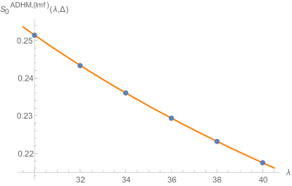
Figure 5: Blue dots represent the numerical values of $S_{0}^{\text{ADHM,(lmf)}}(\lambda,\boldsymbol{\Delta})$ and the orange line corresponds to the fitting curve in (105) for the configuration (102).

Both Table 1 and Fig. 5 strongly support that the LinearModelFit (105) captures the analytic behavior of the real part of the planar effective action precisely. Based on this observation, substituting (105) with (106) back into (90), we arrive at the analytic expression for the planar free energy (91). A similar numerical analysis has been implemented for different $(\lambda,\boldsymbol{\Delta})$ configurations in Appendix C.1, which finally confirms the ADHM planar free energy (91) for general $(\lambda,\boldsymbol{\Delta})$ configurations.

Note that in this subsection we have focused on the configuration (102) where we do not know the analytic form of $\mathfrak{c}^{\text{ADHM}}(\boldsymbol{\Delta})$ yet; hence we provided the numerical estimation $\mathfrak{c}^{\text{ADHM,(lmf)}}(\boldsymbol{\Delta})$ in Table 1 instead of the unknown error ratio $R^{\mathfrak{c}}(\boldsymbol{\Delta})$. In Appendix C.1 we also consider the cases satisfying the extra constraints $\Delta_{3}=1$ where the analytic form of $\mathfrak{c}^{\text{ADHM}}(\boldsymbol{\Delta})$ is successfully confirmed as (92).

4.1.2 $V^{5,2}$ theory

The numerical analysis described in the beginning of this subsection 4.1 yields the $V^{5,2}$ planar free energy consistent with the universal form (1), namely

$$\begin{split}F_{0}^{V^{5,2}}(\lambda,\boldsymbol{\Delta})&=\frac{4\pi\sqrt{\widetilde{\Delta}_{1}\widetilde{\Delta}_{2}\widetilde{\Delta}_{3}\widetilde{\Delta}_{4}}}{3}\frac{\Big{(}\lambda-\frac{1-(\widetilde{\Delta}_{1}+\widetilde{\Delta}_{2})+\widetilde{\Delta}_{1}\widetilde{\Delta}_{2}}{12\widetilde{\Delta}_{1}\widetilde{\Delta}_{2}}\Big{)}^{\frac{3}{2}}}{\lambda^{2}}+\frac{\mathfrak{c}^{V^{5,2}}(\boldsymbol{\Delta})}{\lambda^{2}}\\ &\quad+\lambda^{-1}{\rm i}\pi(\widetilde{\Delta}-\Delta)\chi+\mathcal{O}(e^{-\#\sqrt{\lambda}})\,,\\ \end{split}$$ (108)

where the analytic expression of $\mathfrak{c}^{V^{5,2}}(\boldsymbol{\Delta})$ has not yet been known. As in the ADHM theory case, the planar free energy (108) is valid to all orders in the large $\lambda$ expansion up to exponentially suppressed non-perturbative corrections and consistent with the result from an analytic approach (56). We leave a more detailed numerical analysis on non-perturbative corrections for future research.

What is different from the ADHM theory case is that the analytic expression (108) has not yet been known even for the superconformal configuration (9) since the free Fermi-gas approach Marino:2011eh ; Hatsuda:2014vsa does not apply to the $V^{5,2}$ theory. It would be very interesting to derive the $V^{5,2}$ planar free energy (108) analytically and we will comment on this open question further in section 5 and 6.

Numerical data that support the analytic expression for the $V^{5,2}$ planar free energy (108) is provided in Appendix C.2. Here we focus on a particular set of $(\lambda,\boldsymbol{\Delta})$ configuration with the superconformal values (9), namely

$$\lambda\in\{30,32,34,36,38,40\}\,,\quad\Delta_{I}=(\frac{2}{3},\frac{2}{3},\frac{2}{3})\,,\quad\chi=0\,,\quad(\Delta,\widetilde{\Delta})=(\frac{1}{3},\frac{1}{3})\,,$$ (109)

and show that the corresponding numerical analysis leads to the expression (108).

As we did in the previous subsection 4.1.1 for the ADHM theory, we first improve the LinearModelFit (89) as (104) based on the same observation (103) for universal logarithmic coefficients. We then LinearModelFit the numerical values of $S_{0}^{V^{5,2}}(\lambda,\boldsymbol{\Delta})$ in the improved fitting (104) with respect to $\lambda$, employing two fitting functions as

$$S_{0}^{V^{5,2},\text{(lmf)}}(\lambda,\boldsymbol{\Delta})=\mathfrak{b}^{V^{5,2},\text{(lmf)}}(\boldsymbol{\Delta})\frac{\Big{(}\lambda-\frac{1-(\widetilde{\Delta}_{1}+\widetilde{\Delta}_{2})+\widetilde{\Delta}_{1}\widetilde{\Delta}_{2}}{12\widetilde{\Delta}_{1}\widetilde{\Delta}_{2}}\Big{)}^{\frac{3}{2}}}{\lambda^{2}}+\mathfrak{c}^{V^{5,2},\text{(lmf)}}(\boldsymbol{\Delta})\frac{1}{\lambda^{2}}\,.$$ (110)

The resulting numerical estimation $\mathfrak{b}^{V^{5,2},\text{(lmf)}}(\boldsymbol{\Delta})$ turns out to be consistent with the analytic result (56) as

$$\mathfrak{b}^{V^{5,2},\text{(lmf)}}(\boldsymbol{\Delta})\simeq\mathfrak{b}^{V^{5,2}}(\boldsymbol{\Delta})\equiv\frac{4\pi\sqrt{\widetilde{\Delta}_{1}\widetilde{\Delta}_{2}\widetilde{\Delta}_{3}\widetilde{\Delta}_{4}}}{3}\,.$$ (111)

The error ratio for the estimate (111) defined as (107) and the standard errors in the LinearModelFit (110) are presented in Table 2.

$R^{V^{5,2},\mathfrak{b}}(\boldsymbol{\Delta})$	$\sigma^{V^{5,2},\mathfrak{b}}(\boldsymbol{\Delta})$	$\mathfrak{c}^{V^{5,2},\text{(lmf)}}(\boldsymbol{\Delta})$	$\sigma^{V^{5,2},\mathfrak{c}}(\boldsymbol{\Delta})$
$2.062\times 10^{-17}$	$1.219\times 10^{-17}$	$0.065067276994384483579$	$2.416\times 10^{-15}$

Table 2: Fitting data for the $V^{5,2}$ planar free energy for the configuration (109). Small values of error ratios and standard errors imply that the LinearModelFit (110) is consistent with a true analytic behavior.

See also Fig. 6 for the LinearModelFit (110) compared with numerical data points.

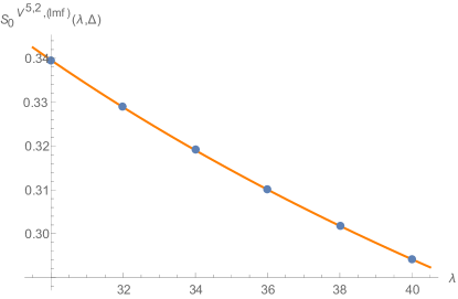
Figure 6: Blue dots represent the numerical values of $S_{0}^{V^{5,2},\text{(lmf)}}(\lambda,\boldsymbol{\Delta})$ and the orange line corresponds to the fitting curve in (110) for the configuration (109).

Both Table 2 and Fig. 6 strongly support that the LinearModelFit (110) captures the analytic behavior of the real part of the planar effective action precisely. Based on this observation, substituting (110) with (111) back into (90), we arrive at the analytic expression for the planar free energy (108). Various other $(\lambda,\boldsymbol{\Delta})$ configurations have been explored in a similar manner in Appendix C.2 and all the results support the $V^{5,2}$ planar free energy (108).

4.2 2-node

For the 2-node theories, the numerical analysis proceeds as follows.

1. Derive the saddle point equations

   $$0 =\frac{N}{\lambda}\frac{{\rm i}}{2\pi}\mu_{i}+\sum_{j=1\,(\neq i)}^{N}\coth\frac{\mu_{i}-\mu_{j}}{2}$$

   $$\quad+\sum_{a=1}^{4}\sum_{j=1}^{N}\bigg{(}\frac{\Delta_{a}-1}{2}-{\rm i}\sigma_{a}\frac{\mu_{i}-\nu_{j}}{4\pi}\bigg{)}\coth(\frac{\mu_{i}-\nu_{j}}{2}-{\rm i}\sigma_{a}\pi(1-\Delta_{a}))$$

   $$\quad+\frac{N}{\lambda_{\mu}}\bigg{(}\frac{\Delta-1}{2}-{\rm i}\frac{\mu_{i}}{4\pi}\bigg{)}\coth\bigg(\frac{\mu_{i}}{2}-{\rm i}\pi(1-\Delta)\bigg{missing})$$

   $$\quad+\frac{N}{\lambda_{\nu}}\bigg{(}\frac{\Delta-1}{2}+{\rm i}\frac{\mu_{i}}{4\pi}\bigg{)}\coth\bigg(\frac{\mu_{i}}{2}+{\rm i}\pi(1-\Delta)\bigg{missing})\,,$$ (112a)

   $$0 =-\frac{N}{\lambda}\frac{{\rm i}}{2\pi}\nu_{i}+\sum_{j=1\,(\neq i)}^{N}\coth\frac{\nu_{i}-\nu_{j}}{2}$$

   $$\quad+\sum_{a=1}^{4}\sum_{j=1}^{N}\bigg{(}\frac{\Delta_{a}-1}{2}+{\rm i}\sigma_{a}\frac{\nu_{i}-\mu_{j}}{4\pi}\bigg{)}\coth(\frac{\nu_{i}-\mu_{j}}{2}+{\rm i}\sigma_{a}\pi(1-\Delta_{a}))$$

   $$\quad+\frac{N}{\lambda_{\nu}}\bigg{(}\frac{\Delta-1}{2}-{\rm i}\frac{\nu_{i}}{4\pi}\bigg{)}\coth\bigg(\frac{\nu_{i}}{2}-{\rm i}\pi(1-\Delta)\bigg{missing})$$

   $$\quad+\frac{N}{\lambda_{\mu}}\bigg{(}\frac{\Delta-1}{2}+{\rm i}\frac{\nu_{i}}{4\pi}\bigg{)}\coth\bigg(\frac{\nu_{i}}{2}+{\rm i}\pi(1-\Delta)\bigg{missing})\,,$$ (112b)

   by taking the 1st derivative of the effective action (58) with respect to the gauge holonomies under the constraints (61). Find a numerical solution $\{\boldsymbol{\mu}^{\star},\boldsymbol{\nu}^{\star}\}$ to the saddle point equation (112) for given $(N,\lambda,\boldsymbol{\Delta})$ configurations using the FindRoot in Mathematica at WorkingPrecision 200, employing the leading order solution (73) or (77) as initial conditions.

2. Evaluate the on-shell effective action

   $$S^{\text{2-node}}[\boldsymbol{\mu}^{\star},\boldsymbol{\nu}^{\star};N,\lambda,\boldsymbol{\Delta}]$$ (113)

   by substituting the numerical solution $\{\boldsymbol{\mu}^{\star},\boldsymbol{\nu}^{\star}\}$ into the effective action (58). In this step we confirmed that the imaginary part of the on-shell effective action vanishes for all the examples of our interest listed in subsection 2.2; recall that we focus on the superconformal configuration for the $N^{0,1,0}$/$Q^{1,1,1}$ theories.

3. LinearModelFit the on-shell effective action (113) with respect to large values of $N$ ($100\sim 350$ in step of $10$) for given $(\lambda,\boldsymbol{\Delta})$ configurations as

   $$\begin{split}S^{\text{2-node}}[\boldsymbol{\mu}^{\star},\boldsymbol{\nu}^{\star};N,\lambda,\boldsymbol{\Delta}]&=S_{0}^{\text{2-node,(lmf)}}(\lambda,\boldsymbol{\Delta})N^{2}+S_{\text{1/2-log}}^{\text{2-node,(lmf)}}(\lambda,\boldsymbol{\Delta})N\log N\\ &\quad+S_{1/2}^{\text{2-node,(lmf)}}(\lambda,\boldsymbol{\Delta})N+S_{\text{1-log}}^{\text{2-node,(lmf)}}(\lambda,\boldsymbol{\Delta})\log N\\ &\quad+\sum_{\ell=0}^{18}S_{\ell/2+1}^{\text{2-node,(lmf)}}(\lambda,\boldsymbol{\Delta})N^{-\ell}\,,\end{split}$$ (114)

   as we did in the 1-node examples. According to the formula (60), reading off the coefficient of the $N^{2}$ leading term in the LinearModelFit (114) yields the numerical value of the planar free energy as

   $$F_{0}^{\text{2-node}}(\lambda,\boldsymbol{\Delta})=S_{0}^{\text{2-node,(lmf)}}(\lambda,\boldsymbol{\Delta})\,.$$ (115)

4. Repeating the above 1-3 steps for various $(\lambda,\boldsymbol{\Delta})$ configurations, deduce the analytic expression of the planar free energy $F_{0}^{\text{2-node}}(\lambda,\boldsymbol{\Delta})$ as a function of the ’t Hooft coupling $\lambda$ and the $R$-charges $\boldsymbol{\Delta}$.

The final results and details involved in the above-described numerical analysis will be presented below for the ABJM, $N^{0,1,0}$, and $Q^{1,1,1}$ theories in order. As in the 1-node cases, we provide the final results first and then explain how the numerical data support them through the above procedure.

4.2.1 ABJM theory

Applying the numerical analysis described above to the ABJM theory, we obtain the ABJM planar free energy

$$\begin{split}F_{0}^{\text{ABJM}}(\lambda,\boldsymbol{\Delta})&=\frac{4\pi\sqrt{2\Delta_{1}\Delta_{2}\Delta_{3}\Delta_{4}}}{3}\frac{(\lambda-\frac{1}{24})^{\frac{3}{2}}}{\lambda^{2}}+\frac{\mathfrak{c}^{\text{ABJM}}(\boldsymbol{\Delta})}{\lambda^{2}}+\mathcal{O}(e^{-\#\sqrt{\lambda}})\,,\\ \end{split}$$ (116)

where the analytic expression of $\mathfrak{c}^{\text{ABJM}}(\boldsymbol{\Delta})$ has been deduced as

$$\mathfrak{c}^{\text{ABJM}}(\boldsymbol{\Delta}) =\frac{\zeta(3)}{8\pi^{2}}\Bigg{[}4-\sum_{a=1}^{4}\Delta_{a}^{2}-4\sum_{a=1}^{4}\frac{\Delta_{1}\Delta_{2}\Delta_{3}\Delta_{4}}{\Delta_{a}}$$ (117)

$$\kern 30.00005pt~{}~{}+\frac{(\Delta_{1}+\Delta_{3}-\Delta_{2}-\Delta_{4})^{2}(\Delta_{1}+\Delta_{4}-\Delta_{2}-\Delta_{3})^{2}}{4(\Delta_{1}+\Delta_{3})(\Delta_{1}+\Delta_{4})(\Delta_{2}+\Delta_{3})(\Delta_{2}+\Delta_{4})}\sum_{a=1}^{4}\frac{\Delta_{1}\Delta_{2}\Delta_{3}\Delta_{4}}{\Delta_{a}}\Bigg{]}\,.$$

The result (116) again takes the universal form (1) as in the 1-node cases. Several comments on the ABJM planar free energy (116) are as follows.

• The ABJM planar free energy (116) is valid to all orders in the large $\lambda$ expansion up to exponentially suppressed non-perturbative corrections, and consistent with the result from a saddle point approximation (80) as expected.

• The ABJM planar free energy (116) is consistent with the results from the free Fermi-gas approach of Marino:2011eh and Nosaka:2015iiw , where the former focuses on the superconformal configuration $\Delta_{a}=\frac{1}{2}$ (see Fuji:2011km for an alternative derivation) and the latter generalizes the former under the weaker constraint

  $$\Delta_{1}+\Delta_{3}=1\qquad\text{or}\qquad\Delta_{1}+\Delta_{4}=1\,.$$ (118)

  To be more explicit, the ABJM free energy was obtained under the constraints (118) via the free Fermi-gas approach for a finite $k=N/\lambda$ as Nosaka:2015iiw

  $$F^{\text{ABJM}}(N,\lambda,\boldsymbol{\Delta})\Big{|}_{\text{(\ref{ABJM:special})}} =-\log\text{Ai}\Big{[}C^{-1/3}(N-B)\Big{]}-\frac{1}{3}\log C+\frac{1}{4}\sum_{a=1}^{4}\mathcal{A}(2\Delta_{a}k)$$

  $$\quad+\mathcal{O}(e^{-\sqrt{N}})\,,$$ (119a)

  $$C =\frac{1}{8\pi^{2}k\Delta_{1}\Delta_{2}\Delta_{3}\Delta_{4}}\,,$$ (119b)

  $$B =\frac{k}{24}+\frac{1}{12k}\bigg{(}\frac{1-\frac{1}{4}\sum_{a=1}^{4}\Delta_{a}^{2}}{\Delta_{1}\Delta_{2}\Delta_{3}\Delta_{4}}-\sum_{a=1}^{4}\frac{1}{\Delta_{a}}\bigg{)}\,.$$ (119c)

  One can check that (119) is consistent with the planar free energy (116) we obtained via the numerical analysis in the IIA string theory limit under the constraints (118), using the asymptotic expansion of the Airy function (100). But our planar free energy expression (116) has been obtained without imposing the constraints (118), which motivates an appropriate generalization of the Airy formula (119) to generic $R$-charge configurations as in Bobev:2022jte ; Bobev:2022eus ; Hristov:2022lcw . We will comment further on this point in section 5.

• To deduce the analytic expression (117) based on numerical data, we have employed the known result Nosaka:2015iiw

  $$\mathfrak{c}^{\text{ABJM}}(\boldsymbol{\Delta})\Big{|}_{\text{(\ref{ABJM:special})}}=\frac{\zeta(3)}{8\pi^{2}}\sum_{a=1}^{4}\Delta_{a}^{2}$$ (120)

  together with the symmetry that the free energy is invariant under

  $$\Delta_{1}\leftrightarrow\Delta_{2}\,,\qquad\Delta_{3}\leftrightarrow\Delta_{4}\,,\qquad(\Delta_{1},\Delta_{2})\leftrightarrow(\Delta_{3},\Delta_{4})\,,$$ (121)

  originating from the structure of the matrix model (10). Note that the 2nd line of (117) vanishes under the special constraint (118), which is required to employ the free Fermi-gas formalism, and respects the symmetry (121). But it does not respect the full permutation symmetry among $\Delta_{a}$, which is reminiscent of the observation made in Chester:2021gdw for the exact partition function with small $(N,k)$ values.

• As in the ADHM theory case, numerical precision is not good enough to analyze exponentially suppressed terms. These non-perturbative corrections are supposed to capture the WS instanton behaviors in a dual IIA string theory side, see Cagnazzo:2009zh ; Drukker:2010nc ; Hatsuda:2012dt ; Nosaka:2015iiw ; Gautason:2023igo ; Beccaria:2023ujc ; Nosaka:2024gle for example. We leave a complete numerical analysis on such instanton corrections for future research.

Numerical data that support the analytic expression for the ABJM planar free energy (116) is provided in Appendix C.3. Here we focus on a particular set of $(\lambda,\boldsymbol{\Delta})$ configuration

$$\lambda\in\{30,32,34,36,38,40\}\,,\qquad\Delta_{a}=(\frac{3}{5},\frac{3}{10},\frac{9}{10},\frac{2}{10})\,,$$ (122)

and show that the corresponding numerical analysis described in the beginning of this subsection 4.2 is indeed consistent with the expression (116). Note that (122) does not satisfy the special constraint (118) employed in Nosaka:2015iiw so there is no known Airy formula like (119) for the free energy with the configuration (122); only the $\lambda^{-1/2}$ leading order (75) has been known so far in the literature Jafferis:2011zi , which is improved to the first subleading correction of order $\lambda^{-3/2}$ in (80) analytically and extended to all orders in the large $\lambda$ expansion as (116) via numerical analysis.

The first step is to observe universal logarithmic coefficients in the LinearModelFit with respect to $N$ (114) as in the 1-node examples, namely

$$S_{\text{1/2-log}}^{\text{2-node,(lmf)}}(\lambda,\boldsymbol{\Delta})\simeq-2\,,\qquad S_{\text{1-log}}^{\text{2-node,(lmf)}}(\lambda,\boldsymbol{\Delta})\simeq-\frac{1}{6}\,.$$ (123)

Subtracting these logarithmic terms from the numerical values of the on-shell effective action improves the LinearModelFit (114) as

$$S^{\text{2-node}}[\boldsymbol{\mu}^{\star};N,\lambda,\boldsymbol{\Delta}]+2N\log N+\frac{1}{6}\log N =S_{0}^{\text{2-node,(lmf)}}(\lambda,\boldsymbol{\Delta})N^{2}+S_{1/2}^{\text{2-node,(lmf)}}(\lambda,\boldsymbol{\Delta})N$$

$$\quad+\sum_{\ell=0}^{20}S_{\ell/2+1}^{\text{2-node,(lmf)}}(\lambda,\boldsymbol{\Delta})N^{-\ell}\,.$$ (124)

We then LinearModelFit the improved numerical estimations for the $N^{2}$ leading order coefficients with respect to $\lambda$, employing two fitting functions as

$$S_{0}^{\text{ABJM,(lmf)}}(\lambda,\boldsymbol{\Delta})=\mathfrak{b}^{\text{ABJM,(lmf)}}(\boldsymbol{\Delta})\frac{(\lambda-\frac{1}{24})^{\frac{3}{2}}}{\lambda^{2}}+\mathfrak{c}^{\text{ABJM,(lmf)}}(\boldsymbol{\Delta})\frac{1}{\lambda^{2}}\,.$$ (125)

The numerical fitting coefficients turn out to be consistent with the analytic expression (116) as

$$\begin{split}\mathfrak{b}^{\text{ABJM,(lmf)}}(\boldsymbol{\Delta})&\simeq\mathfrak{b}^{\text{ABJM}}(\boldsymbol{\Delta})\equiv\frac{4\pi\sqrt{2\Delta_{1}\Delta_{2}\Delta_{3}\Delta_{4}}}{3}\,,\\ \mathfrak{c}^{\text{ABJM,(lmf)}}(\boldsymbol{\Delta})&\simeq\mathfrak{c}^{\text{ABJM}}(\boldsymbol{\Delta})\,,\end{split}$$ (126)

where the latter coefficient $\mathfrak{c}^{\text{ABJM}}(\boldsymbol{\Delta})$ is defined in (117). The error ratios for the estimates (126) defined by

$$R^{\mathfrak{b}}(\boldsymbol{\Delta})\equiv\frac{\mathfrak{b}^{\text{2-node,(lmf)}}(\boldsymbol{\Delta})-\mathfrak{b}^{\text{2-node}}(\boldsymbol{\Delta})}{\mathfrak{b}^{\text{2-node}}(\boldsymbol{\Delta})}\,,\quad R^{\mathfrak{c}}(\boldsymbol{\Delta})\equiv\frac{\mathfrak{c}^{\text{2-node,(lmf)}}(\boldsymbol{\Delta})-\mathfrak{c}^{\text{2-node}}(\boldsymbol{\Delta})}{\mathfrak{c}^{\text{2-node}}(\boldsymbol{\Delta})}\,,$$ (127)

and the standard errors in the LinearModelFit (125) are presented in Table 3.

$R^{\text{ABJM},\mathfrak{b}}(\boldsymbol{\Delta})$	$\sigma^{\text{ABJM},\mathfrak{b}}(\boldsymbol{\Delta})$	$R^{\text{ABJM},\mathfrak{c}}(\boldsymbol{\Delta})$	$\sigma^{\text{ABJM},\mathfrak{c}}(\boldsymbol{\Delta})$
$1.550\times 10^{-11}$	$3.139\times 10^{-12}$	$-2.056\times 10^{-7}$	$6.213\times 10^{-10}$

Table 3: Fitting data for the ABJM planar free energy for the configuration (122). Small values of error ratios and standard errors imply that the LinearModelFit (125) is consistent with a true analytic behavior.

See also Fig. 7 for the LinearModelFit (125) compared with numerical data points.

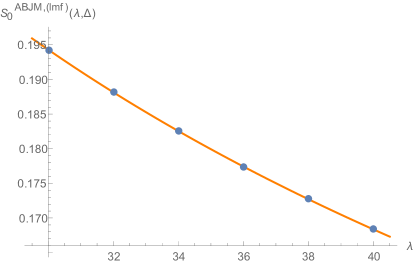
Figure 7: Blue dots represent the numerical values of $S_{0}^{\text{ABJM,(lmf)}}(\lambda,\boldsymbol{\Delta})$ and the orange line corresponds to the fitting curve in (125) for the configuration (122).

Both Table 3 and Fig. 7 strongly support that the LinearModelFit (125) captures the analytic behavior of the planar effective action precisely. Based on this observation, substituting (125) with (126) back into (115), we obtain the analytic expression for the planar free energy (116). A similar numerical analysis for various other $(\lambda,\boldsymbol{\Delta})$ configurations also confirms the ABJM planar free energy (116), see Appendix C.3 for details.

4.2.2 $N^{0,1,0}$ theory

The numerical analysis described in the beginning of this subsection 4.2 yields the $N^{0,1,0}$ planar free energy ($\alpha\equiv r/k$)

$$\begin{split}F_{0}^{N^{0,1,0}}(\lambda,\alpha)=\frac{2(1+\alpha)\pi}{3\sqrt{2+\alpha}}\frac{(\lambda-\frac{2-3\alpha}{48})^{\frac{3}{2}}}{\lambda^{2}}+\frac{\mathfrak{c}^{N^{0,1,0}}(\alpha)}{\lambda^{2}}+\mathcal{O}(e^{-\#\sqrt{\lambda}})\\ \end{split}$$ (128)

for the superconformal configuration (16), where the analytic expression of $\mathfrak{c}^{N^{0,1,0}}(\alpha)$ has not yet been known. The result (128) is not new and can be read off from the known Airy formula for the $S^{3}$ partition function Marino:2011eh ; Bobev:2023lkx in the IIA string theory limit. Hence in this example our numerical analysis serves only as a consistency check, and therefore we relegate all the details involved in the numerical analysis to Appendix C.4. It would be very interesting to investigate the $N^{0,1,0}$ planar free energy beyond the reach of the free Fermi-gas formalism that yields the Airy formula, for instance by removing the constraint $r_{1}=r_{2}$ introduced in (17), and see if the planar free energy still takes the universal form (1). See Appendix B.5 for more detailed discussion on this point.

4.2.3 $Q^{1,1,1}$ theory

Applying the numerical analysis summarized in the beginning of this subsection 4.2 to the $Q^{1,1,1}$ theory at the superconformal configuration (21), we obtain the $Q^{1,1,1}$ planar free energy

$$F_{0}^{Q^{1,1,1}}(\lambda)=\frac{4\pi}{3\sqrt{3}}\frac{(\lambda+\frac{1}{12})^{\frac{3}{2}}}{\lambda^{2}}+\frac{\mathfrak{c}^{Q^{1,1,1}}}{\lambda^{2}}+\mathcal{O}(e^{-\#\sqrt{\lambda}})\,,$$ (129)

where the analytic expression of $\mathfrak{c}^{Q^{1,1,1}}$ has not yet been deduced. As in the previous examples, the planar free energy (129) is valid to all orders in the large $\lambda$ expansion up to exponentially suppressed non-perturbative corrections, and consistent with the result from an analytic approach (85). We leave a more detailed numerical analysis on non-perturbative corrections for future research.

Similar to the $V^{5,2}$ theory case, the analytic expression (129) has not yet been known even for the superconformal configuration (21) since the free Fermi-gas formalism is not applicable to the matrix model for the $S^{3}$ partition function of the $Q^{1,1,1}$ theory. Hence the analytic derivation of a simple expression (129), again consistent with the universal form (1), remains an interesting open problem and we will comment on this issue in section 5.

To derive the $Q^{1,1,1}$ planar free energy (129), we implement the numerical analysis for $\lambda=30\sim 50$ (in step of $2$). As in the ABJM theory case explored in subsection 4.2.1, we first improve the LinearModelFit (114) as (124) by subtracting the universal logarithmic coefficients (123). We then LinearModelFit the improved numerical values of $S_{0}^{Q^{1,1,1}}(\lambda)$ in (124) with respect to $\lambda$, employing two fitting functions as

$$S_{0}^{Q^{1,1,1},\text{(lmf)}}(\lambda)=\mathfrak{b}^{Q^{1,1,1},\text{(lmf)}}\frac{(\lambda+\frac{1}{12})^{\frac{3}{2}}}{\lambda^{2}}+\mathfrak{c}^{Q^{1,1,1},\text{(lmf)}}\frac{1}{\lambda^{2}}\,.$$ (130)

The fitting coefficient $\mathfrak{b}^{Q^{1,1,1},\text{(lmf)}}$ is confirmed to be given as

$$\mathfrak{b}^{Q^{1,1,1},\text{(lmf)}}\simeq\mathfrak{b}^{Q^{1,1,1}}\equiv\frac{4\pi}{3\sqrt{3}}\,,$$ (131)

which is consistent with the analytic results (85). The error ratio for the estimate (131) defined as (127) and the standard errors in the LinearModelFit (130) are presented in Table 4.

$R^{Q^{1,1,1},\mathfrak{b}}$	$\sigma^{Q^{1,1,1},\mathfrak{b}}$	$\mathfrak{c}^{Q^{1,1,1},\text{(lmf)}}$	$\sigma^{Q^{1,1,1},\mathfrak{c}}$
$2.263\times 10^{-11}$	$1.291\times 10^{-11}$	$0.060896898392804042312$	$2.917\times 10^{-9}$

Table 4: Fitting data for the $Q^{1,1,1}$ planar free energy for $\lambda=30\sim 50$ (in step of $2$). Small values of error ratios and standard errors imply that the LinearModelFit (130) is consistent with a true analytic behavior.

See also Fig. 8 for the LinearModelFit (130) compared with numerical data points.

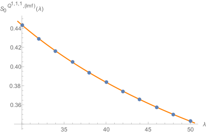
Figure 8: Blue dots represent the numerical values of $S_{0}^{Q^{1,1,1},\text{(lmf)}}(\lambda)$ and the orange line corresponds to the fitting curve in (130).

Both Table 4 and Fig. 8 confirm that the LinearModelFit (130) captures the analytic behavior of the planar effective action precisely. Based on this observation, substituting (130) with (131) back into (115), we arrive at the analytic expression for the planar free energy (129).

5 Airy conjectures

In this section we discuss Airy formulae for the $S^{3}$ partition functions of $\mathcal{N}=2$ holographic SCFTs introduced in section 2. In subsection 5.1 we first compare the planar free energies obtained in the previous sections 3 and 4 with the known Airy conjectures for the $S^{3}$ partition functions of the ABJM/ADHM theories. In subsection 5.2 we move on to other examples, and conjecture new Airy formulae for the $S^{3}$ partition functions based on their planar free energies. In due process, the universal form of the planar free energy (1), which we repeat here as

$$F^{\text{SCFT}}_{0}(\lambda)=\mathfrak{b}^{\text{SCFT}}\big{(}\lambda-B^{\text{SCFT}}\big{)}^{\frac{3}{2}}+\frac{\mathfrak{c}^{\text{SCFT}}}{\lambda^{2}}+\mathcal{O}(e^{-\#\sqrt{\lambda}})\,,$$ (132)

will play the key role. In (132) the theory-dependent constants $\mathfrak{b}^{\text{SCFT}}$, $\mathfrak{c}^{\text{SCFT}}$, and $B^{\text{SCFT}}$ can be read off from the results in the previous section 4 for various examples of our interest.

5.1 Comparison with the known Airy conjectures

To begin with, recall that the Airy formula for the ABJM $S^{3}$ partition function (119), derived via the free Fermi-gas formalism under the extra constraint (118) in Nosaka:2015iiw , has recently been extended to generic $R$-charges under the original superpotential marginality constraint (12) as Bobev:2022jte ; Bobev:2022eus ; Hristov:2022lcw

$$F^{\text{ABJM}}(N,\lambda,\boldsymbol{\Delta}) =-\log\text{Ai}\Big{[}C^{-1/3}(N-B)\Big{]}-\frac{1}{3}\log C+\mathcal{A}^{\text{ABJM}}(k,\boldsymbol{\Delta})+\mathcal{O}(e^{-\sqrt{N}})\,,$$ (133a)

$$C =\frac{1}{8\pi^{2}k\Delta_{1}\Delta_{2}\Delta_{3}\Delta_{4}}\,,$$ (133b)

$$B =\frac{k}{24}+\frac{1}{12k}\bigg{(}\frac{1-\frac{1}{4}\sum_{a=1}^{4}\Delta_{a}^{2}}{\Delta_{1}\Delta_{2}\Delta_{3}\Delta_{4}}-\sum_{a=1}^{4}\frac{1}{\Delta_{a}}\bigg{)}\,,$$ (133c)

where the analytic expression for the $N$-independent contribution $\mathcal{A}^{\text{ABJM}}(k,\boldsymbol{\Delta})$ is left unknown. The conjecture (133) has not yet been analytically proven, but passed various non-trivial consistency checks Bobev:2022eus . Our planar free energy result (116) provides a new independent non-trivial test for the Airy conjecture (133) by confirming that the $\frac{k}{24}$ piece in (133c) is valid for generic $R$-charges even without the constraint (118). Furthermore, the planar free energy (116) tells us that the large $k$ expansion of the unknown function $\mathcal{A}^{\text{ABJM}}(k,\boldsymbol{\Delta})$ is supposed to be given as

$$\mathcal{A}^{\text{ABJM}}(k,\boldsymbol{\Delta})=\mathfrak{c}^{\text{ABJM}}(\boldsymbol{\Delta})k^{2}+o(k^{2})\,,$$ (134)

where the analytic expression for the coefficient $\mathfrak{c}^{\text{ABJM}}(\boldsymbol{\Delta})$ is determined explicitly in (117).

Another Airy conjecture we would like to compare with our planar free energy results is for the $S^{3}$ partition function of the ADHM theory with an $\mathcal{N}=4$ symmetry breaking mass term Minahan:2021pfv ; Bobev:2023lkx . Turning on the $\mathcal{N}=4$ symmetry breaking mass parameter $\mathfrak{m}$ corresponds to choosing a specific configuration of $R$-charges in the 1-node matrix model (3), namely Bobev:2023lkx

$$\Delta_{1}=\Delta_{2}=\Delta=\widetilde{\Delta}=\frac{1-{\rm i}\mathfrak{m}}{2}\,,\qquad\Delta_{3}=1+{\rm i}\mathfrak{m}\,,\qquad\Delta_{m}=0\,,$$ (135)

and the corresponding Airy conjecture for the $S^{3}$ partition function is given as Bobev:2023lkx

$$F^{\text{ADHM}}(N,\lambda,\boldsymbol{\Delta})\Big{|}_{\text{(\ref{ADHM:N=4})}} =-\log\text{Ai}[C^{-\frac{1}{3}}(N-B)]-\frac{1}{3}\log C+\mathcal{A}+\mathcal{O}(e^{-\sqrt{N}})\,,$$ (136a)

$$C =\frac{2}{\pi^{2}N_{f}}\frac{1}{(1+{\rm i}\mathfrak{m})^{2}(1-{\rm i}\mathfrak{m})^{2}}\,,$$ (136b)

$$B \overset{!}{=}N_{f}\bigg{(}\frac{1}{24}-\frac{1+3\mathfrak{m}^{2}}{6(1+{\rm i}\mathfrak{m})^{2}(1-{\rm i}\mathfrak{m})^{2}}\bigg{)}+\frac{1}{N_{f}}\frac{3+\mathfrak{m}^{2}}{6(1+{\rm i}\mathfrak{m})^{2}(1-{\rm i}\mathfrak{m})^{2}}\,,$$ (136c)

where the $N$-independent constant $\mathcal{A}$ has not yet been conjectured. Note that (136) is beyond the reach of the Airy formula (96) derived via the free Fermi-gas formalism in Chester:2023qwo since the configuration (135) is distinguished from (95). Unlike the ABJM Airy conjecture discussed above, in this case our planar free energy result (91) is not consistent with the Airy formula (136) at the planar level in the ’t Hooft limit under the parameter identifications (49) and (135); the key difference is between the shift of the ’t Hooft coupling in (91) and the first term in the $B$ parameter (136c). This implies that, even though the conjecture (136) passed various consistency checks Bobev:2023lkx , it does not capture the $S^{3}$ partition function precisely. It is non-trivial to derive the correct Airy formula analytically and thereby fix (136c) in this case, however, since (135) does not satisfy the simplifying constraint $\Delta_{3}=1$ in (95) required for the application of the free Fermi-gas approach. Hence the first step toward addressing this issue is to explore if one can formulate an Airy conjecture for the squashed $S^{3}_{b}$ partition function of the ADHM with the $\mathcal{N}=4$ symmetry breaking mass term as in Bobev:2023lkx , but in a way consistent with our planar free energy result (91). A useful guidance for this research direction will be briefly discussed in the next subsection.

5.2 New Airy conjectures

For other holographic SCFTs considered in this paper whose $S^{3}$ partition functions are beyond the scope of the free Fermi-gas formalism — namely the ADHM theory with the most general $R$-charges, the $V^{5,2}$ theory, the $N^{0,1,0}$ theory with generic $r_{1,2}$ values, and the $Q^{1,1,1}$ theory — there is no known Airy conjecture for the $S^{3}$ partition function. Motivated by the above observation that our planar free energy calculation provides non-trivial evidence for the Airy conjecture for the ABJM $S^{3}$ partition function with generic $R$-charges, however, we can now formulate an Airy conjecture for such cases employing the universal planar free energy form (132). Below we focus on the ADHM theory with generic $R$-charges and the $V^{5,2}$/$Q^{1,1,1}$ theories in this regard and leave the Airy conjectures for the $N^{0,1,0}$ theory with generic $r_{1,2}$ values for future work.

For the ADHM theory with generic $R$ charges, we can deduce the Airy conjecture based on the planar free energy result (91) and the IR duality between the ADHM theory with $N_{f}=1$ and the ABJM theory with $k=1$ Aharony:2008ug ; Kapustin:2010xq . The resulting conjecture reads

$$F^{\text{ADHM}}(N,\lambda,\boldsymbol{\Delta}) =-\log\text{Ai}[C^{-\frac{1}{3}}(N-B)]-\frac{1}{3}\log C+\mathcal{A}$$

$$\quad+{\rm i}\pi N\Delta_{m}(\widetilde{\Delta}-\Delta)+\mathcal{O}(e^{-\sqrt{N}})\,,$$ (137a)

$$C =\frac{1}{8\pi^{2}N_{f}\widetilde{\Delta}_{1}\widetilde{\Delta}_{2}\widetilde{\Delta}_{3}\widetilde{\Delta}_{4}}\,,$$ (137b)

$$B =\frac{1-2(\widetilde{\Delta}_{1}+\widetilde{\Delta}_{2})+\widetilde{\Delta}_{1}\widetilde{\Delta}_{2}}{24\widetilde{\Delta}_{1}\widetilde{\Delta}_{2}}N_{f}$$

$$\quad-\frac{\widetilde{\Delta}_{1}^{2}+\widetilde{\Delta}_{2}^{2}+5\widetilde{\Delta}_{1}\widetilde{\Delta}_{2}-2(1+\widetilde{\Delta}_{1}\widetilde{\Delta}_{2})(\widetilde{\Delta}_{1}+\widetilde{\Delta}_{2})}{24\widetilde{\Delta}_{1}\widetilde{\Delta}_{2}\widetilde{\Delta}_{3}\widetilde{\Delta}_{4}}\frac{1}{N_{f}}\,,$$ (137c)

where the $N$-independent constant $\mathcal{A}$ is supposed to reproduce (92) and (99) under the corresponding special cases but left unknown in general. The imaginary contribution is read off from the property (94) immediately. The $C$ coefficient and the first $N_{f}$-linear term in the $B$ coefficient are determined unambiguously relying on the planar free energy result (91) and the asymptotic expansion of the Airy function (100). The IR equivalence between the ADHM theory with $N_{f}=1$ and the ABJM theory with $k=1$ is then used to determine the second term in the $B$-coefficient; the ADHM $B$ coefficient (137c) is designed to match the ABJM $B$ coefficient (133c) under $N_{f}=k=1$ and the identification $\widetilde{\Delta}_{a}\leftrightarrow\Delta_{a}$.

One can check that the general ADHM Airy conjecture (137) reproduces the proven Airy formula (96) under the constraint (95a). However, it is not consistent with the Airy conjecture (136) for the $\mathcal{N}=4$ symmetry breaking mass term Bobev:2023lkx as we already commented on in the previous subsection. To be more specific, the inconsistency is captured by

$$\begin{split}B\Big{|}_{(\ref{F:ADHM:Airy:general:B})\,\text{w/}\,(\ref{ADHM:N=4})}-B\Big{|}_{(\ref{F:ADHM:Airy:N=4:B})}=-\frac{{\rm i}\mathfrak{m}^{3}}{8(1+\mathfrak{m}^{2})^{2}}\bigg{(}N_{f}-\frac{1}{N_{f}}\bigg{)}\,,\end{split}$$ (138)

and it would be very interesting to modify the Airy conjecture for the $S^{3}_{b}$ partition function in Bobev:2023lkx incorporating this difference. We leave this problem for future work.

For the $V^{5,2}$/$Q^{1,1,1}$ theories, we first use the recent observation on the relation between the topologically twisted index and the superconformal index of 3d $\mathcal{N}=2$ SCFTs Bobev:2022wem ; Bobev:2024 in conjunction with the structure of the 4-derivative corrections to dual $\mathcal{N}=2$ minimal gauged supergravity Bobev:2020egg ; Bobev:2021oku , which determines the 3d large $N$ partition functions to the first subleading order in the M-theory regime Bobev:2020egg ; Bobev:2021oku ; Bobev:2022wem ; Bobev:2024 . For the $V^{5,2}$/$Q^{1,1,1}$ theories of our interest, the resulting $S^{3}$ free energies are given by Bobev:2024

$$F^{V^{5,2}}(\lambda) =\frac{16\pi\sqrt{N_{f}}}{27}\bigg{[}N^{\frac{3}{2}}-\frac{N_{f}^{2}+15}{32N_{f}}N^{\frac{1}{2}}\bigg{]}+\mathcal{O}(\log N)\,,$$ (139)

$$F^{Q^{1,1,1}}(\lambda) =\frac{4\pi\sqrt{N_{f}}}{3\sqrt{3}}\bigg{[}N^{\frac{3}{2}}+\frac{N_{f}^{2}-3}{8N_{f}}N^{\frac{1}{2}}\bigg{]}+\mathcal{O}(\log N)\,,$$ (140)

where $N_{f}$ is treated as a finite parameter in the large $N$ limit. In the IIA string theory limit where $N$ is taken large with a fixed ’t Hooft coupling $\lambda\equiv N/N_{f}$, these are consistent with the planar free energy results we obtained in (108) and (129) respectively. Now combining (108) with (139), and similarly (129) with (140), we conjecture the Airy formulae for their $S^{3}$ partition functions as (recall $F=-\log Z$)

$$Z^{V^{5,2}}(N,\lambda) =\bigg{(}\frac{81}{64\pi^{2}N_{f}}\bigg{)}^{-\frac{1}{3}}e^{\mathcal{A}^{V^{5,2}}(N_{f})}\text{Ai}\bigg{[}\bigg{(}\frac{81}{64\pi^{2}N_{f}}\bigg{)}^{-\frac{1}{3}}\bigg{(}N-\frac{N_{f}^{2}+15}{48N_{f}}\bigg{)}\bigg{]}(1+\mathcal{O}(e^{-\sqrt{N}}))\,,$$ (141)

$$Z^{Q^{1,1,1}}(N,\lambda) =\bigg{(}\frac{3}{4\pi^{2}N_{f}}\bigg{)}^{-\frac{1}{3}}e^{\mathcal{A}^{Q^{1,1,1}}(N_{f})}\text{Ai}\bigg{[}\bigg{(}\frac{3}{4\pi^{2}N_{f}}\bigg{)}^{-\frac{1}{3}}\bigg{(}N+\frac{N_{f}^{2}-3}{12N_{f}}\bigg{)}\bigg{]}(1+\mathcal{O}(e^{-\sqrt{N}}))\,,$$ (142)

where the $\mathcal{A}$-functions have the following large $N_{f}$ behaviors:

$$\mathcal{A}^{V^{5,2}}(N_{f})=\mathfrak{c}^{V^{5,2}}(\boldsymbol{\Delta})\Big{|}_{\text{(\ref{V52:constraints:sc})}}N_{f}^{2}+o(N_{f}^{2})\,,\qquad\mathcal{A}^{Q^{1,1,1}}(N_{f})=\mathfrak{c}^{Q^{1,1,1}}N_{f}^{2}+o(N_{f}^{2})\,.$$ (143)

In fact, one may derive the above Airy conjectures relying solely on (139) and (140), mimicking the known structures in (96) and (133). This was first done in the work in progress Hong:2024 exploring the squashed 3-sphere partition functions. The important role of our planar free energy calculations (108) and (129), however, is to provide non-trivial evidence for the Airy conjectures to all orders in the large $\lambda$ expansion at the planar level, which is not captured by the previous large $N$ partition functions (139) and (140). It would be very interesting to confirm the Airy conjectures (141) and (142) either beyond the planar level in the IIA string theory limit or beyond the $N^{\frac{1}{2}}$ order in the M-theory limit where $N$ is taken large with a fixed $N_{f}$. In section 6 we will comment on this research direction further.

6 Discussion

We studied the $S^{3}$ partition functions of various 3d $\mathcal{N}=2$ holographic SCFTs arising from the $N$ stack of M2 branes at the tip of the cone over 7d Sasaki-Einstein manifolds, focusing on the planar limit where $N$ is taken large with a fixed ’t Hooft coupling $\lambda$. Based on the matrix model representation of such $S^{3}$ partition functions given from supersymmetric localization, we first employed the saddle point approximation to evaluate the planar $S^{3}$ free energy analytically to the first subleading corrections in the large ’t Hooft coupling limit. These analytic results are then improved to all orders in the large $\lambda$ expansion via numerical analysis. It is remarkable that the resulting planar free energies always take the universal form (132), which we compared with the known Airy conjectures for the ABJM/ADHM theories and furthermore employed to propose new Airy conjectures for the $V^{5,2}$/$Q^{1,1,1}$ theories as well as the ADHM theory with generic $R$-charges. Below we present various open questions.

One of the most pressing tasks is to analytically prove the universal form of the planar free energy (132) that we have confirmed in various $\mathcal{N}=2$ holographic SCFTs arising from the $N$ stack of M2-branes. One may attempt to improve the current saddle point ansatz (36) and (63) which are ignorant of the shift of the ’t Hooft coupling observed in the universal form (132). Another promising approach is to employ the resolvent, whose associated spectral curve in the planar limit can be employed to derive the planar free energy of the corresponding matrix model via appropriate period integrals Ambjorn:1992gw ; DiFrancesco:1993cyw ; Akemann:1996zr ; Dijkgraaf:2002fc ; Aganagic:2002wv ; Ashok:2002bi ; Halmagyi:2003ze , as well-reviewed in Marino:2011nm ; Marino:2016new for our context. Even though the resolvent method was applied only to the superconformal configuration of the ABJM theory among the examples of our interest, considering that the universal form (132) has been observed beyond such a special case, we expect that there must be a systematic approach — the resolvent method or another — for the calculation of the planar free energy of generic $\mathcal{N}=2$ holographic SCFTs with M-theory duals. It would be very interesting to figure out such an analytic method.

Another interesting direction is to extend our analytic/numerical saddle point analysis beyond the planar level by incorporating loop corrections. In principle, one may expect that the $N^{0}$ order corrections in the ’t Hooft limit can be tracked easily by including the 1-loop determinant in a saddle point approximation. There is a subtle issue in the saddle point approximation for the Hermitian matrix model of rank $N$ in the large $N$ expansion Liu:2019tuk ; Liu:2020bih ; Hong:2021bsb , however, which yields a non-vanishing artifact at the linear $N$ order even after incorporating the 1-loop determinant. Exploring higher loop corrections in a saddle point approximation and thereby determining the genus-1 contribution correctly would therefore be a first step in this research direction. In due process, one can also investigate the $\log N$ order and thereby support the characteristic logarithmic behaviors with pure number coefficients employed in the recent work Bobev:2023dwx for a larger class of holographic SCFTs. The results will offer useful guidance to understand stringy loop corrections in a dual IIA string theory path integral in the context of holography, which can be explored alternatively through M-theory, as well as a non-trivial test for the known Airy conjectures for the $S^{3}$ partition functions beyond the planar level.

It would also be intriguing to explore the $S^{3}$ partition functions of more generic $\mathcal{N}=2$ holographic SCFTs dual to the $N$ stack of M2-branes and conjecture new Airy formulae for them. For instance, it is still non-trivial to employ the known methods such as the saddle point approximation (see Appendix B.5 for discussion on this point) and the free Fermi-gas formalism to analyze the $S^{3}$ partition function of the $N^{0,1,0}$ theory with different $r_{1,2}$ values beyond the $\lambda^{-1/2}N^{2}$ leading order in the double scaling limit. Figuring out how to investigate its $S^{3}$ partition function beyond the leading order and then exploring if the subleading structure allows for a new Airy conjecture is therefore an interesting open problem. Extending a similar analysis to generic $\mathcal{N}=2$ holographic SCFTs with M-theory duals would then be a natural follow-up task.

The ultimate question when it comes to the Airy tale is how to prove the conjectured Airy formula for the $S^{3}$ partition functions of various $\mathcal{N}=2$ holographic SCFTs. There are two well-established methods that have been employed to derive the Airy formulae: the free Fermi-gas formalism Marino:2011eh and the chain of dualities relating the matrix model of our interest and the topological string theories Witten:1992fb ; Aganagic:2002wv ; Gopakumar:1998ki ; Ooguri:2002gx ; Bershadsky:1993cx ; Dijkgraaf:2002fc ; Eynard:2007hf ; Marino:2009jd , where the latter is outlined well in Fuji:2011km for the ABJM theory. Their application to the $S^{3}$ partition functions of generic $\mathcal{N}=2$ holographic SCFTs does not seem plausible at this point, however, since both approaches require certain necessary conditions that are not apparently satisfied in various examples of our interest. It would be very interesting if one figures out how to apply these methods in general setting or finds a brand new method, and thereby proves that this class of $\mathcal{N}=2$ holographic SCFTs with M-theory duals always has the 3-sphere partition function captured by an Airy function.

While this manuscript and the aforementioned open questions focus on perturbative contributions to the $S^{3}$ partition function, understanding the non-perturbative behaviors is another important direction in this research program. For example, non-perturbative corrections in the $S^{3}$ partition functions of the ABJM/ADHM theory and their stringy dual descriptions have been analyzed extensively in numerous references Hatsuda:2014vsa ; Cagnazzo:2009zh ; Drukker:2010nc ; Hatsuda:2012dt ; Nosaka:2015iiw ; Gautason:2023igo ; Beccaria:2023ujc ; Nosaka:2024gle . Such a non-perturbative analysis on the field theory side has been restricted to the cases where the perturbatively exact Airy formula is proven via the free Fermi-gas formalism, however, and therefore our numerical saddle point analysis could be a first step toward the non-perturbative analysis for generic $\mathcal{N}=2$ holographic SCFTS without known Airy formulae. To achieve this, improving the precision in the numerics to capture the leading WS instanton corrections of order $\sim e^{-\#\sqrt{\lambda}}$ would be a primary task. Another related question on non-perturbative contributions concerns different saddles in the matrix model and their roles in phase transitions Nosaka:2015bhf ; Nosaka:2016vqf , which would be interesting to explore via the same numerical approach employed in this manuscript.

Motivated by a successful numerical analysis for the $S^{3}$ partition functions of $\mathcal{N}=2$ holographic SCFTs arising from the $N$ stack of M2-branes, it is natural to ask if a similar all order exact (with respect to a large ’t Hooft coupling expansion) result for the planar free energy is available in different classes of holographic SCFTs. One of the promising targets is the 3d SCFTs associated with a non-vanishing Romans mass Gaiotto:2009mv ; Guarino:2015jca , whose $S^{3}$ partition functions have been analyzed in various ways Jafferis:2011zi ; Marino:2011eh ; Suyama:2010hr ; Suyama:2013fua ; Liu:2019tuk ; Hong:2021bsb ; Liu:2021njm . The compact all order expression like (132) has not yet been determined in this class of holographic SCFTs, however, and it would be very interesting if the numerical analysis can enlighten the hidden structure beyond the most recent observation in Liu:2021njm .

Another interesting direction of generalization is to incorporate a non-trivial squashing parameter $b$ in the game. The matrix models capturing the squashed 3-sphere partition functions are given explicitly in the literature Hama:2011ea ; Imamura:2011wg and one can therefore analyze the $S^{3}_{b}$ planar free energy in the same way as we did for the round 3-sphere. One technical obstacle is that the supersymmetric localization results in a matrix model written in terms of a double sine function for the $S^{3}_{b}$ partition function Hama:2011ea ; Imamura:2011wg , not the special $\ell$-function exploited extensively in this manuscript, whose asymptotic expansion is less explicit beyond the leading order. It would be very interesting to explore squashed 3-sphere partition functions beyond the leading order in the large ’t Hooft coupling limit by addressing this technical issue since the result can be employed to support the Airy conjecture involving the squashing parameter Bobev:2022jte ; Bobev:2022eus ; Bobev:2023lkx ; Hristov:2022lcw . The first step towards this research direction will be reported in Hong:2024 .

Lastly, to understand the $S^{3}$ planar free energies valid to all orders in the large ’t Hooft coupling expansion in the context of holographic duality, the primary task is to reproduce the subleading terms from higher derivative corrections on the gravity side. Recall that the leading $\lambda^{-1/2}$ behavior in the planar free energy has been successfully derived from the 2-derivative on-shell action in a dual supergravity side Drukker:2010nc ; Herzog:2010hf ; Cheon:2011vi ; Martelli:2011qj . The starting point for the subleading analysis is therefore to analyze the 8-derivative corrections in Type IIA supergravity or in 11-dimensional supergravity — see Grimm:2017okk ; Ozkan:2024euj for example and references therein — and evaluate their Euclidean on-shell actions on the AdS${}_{4}\times X$ background where the internal manifold $X$ is specified by a dual 3d SCFT of interest, modulo a subtle issue in supergravity on-shell actions upon the Kaluza-Klein compactification Kurlyand:2022vzv ; Beccaria:2023hhi . In due process, it would be very interesting to figure out the origin of the simple universal structure of the planar free energy (132) from the holographic viewpoint. For instance, one may be able to understand a constant shift of the ’t Hooft coupling in the universal form (132) in terms of the renormalization of Newton constant as explored in Bobev:2021oku ; Bobev:2022eus focusing on the ABJM theory. The remaining $\lambda^{-2}$ behavior in (132) might signal the on-shell action of the quartic $R^{4}$ term, considering that its coefficient involves the transcendental number $\zeta(3)$ Gross:1986iv ; Grimm:2017okk ; Ozkan:2024euj and we have encountered the same $\zeta(3)$ factor in the ABJM/ADHM planar free energies. This line of exploration will offer a very concrete research direction towards comprehending string/M-theory beyond the 2-derivative low energy description.

Appendix A Useful functions

The $\ell$-function is defined as

$$\ell(z)\equiv-z\log(1-e^{2\pi{\rm i}z})+\frac{{\rm i}}{2}\bigg{(}\pi z^{2}+\frac{1}{\pi}\text{Li}_{2}(e^{2\pi{\rm i}z})\bigg{)}-\frac{{\rm i}\pi}{12}\,,$$ (144)

see Jafferis:2010un ; Jafferis:2011zi for example. The $\ell$-function has the following inversion properties

$$\begin{split}\exp[\ell(u)]\exp[\ell(-u)]&=1\,,\\ \exp[\ell(\frac{1}{2}+\frac{{\rm i}}{2\pi}u)]\exp[\ell(\frac{1}{2}-\frac{{\rm i}}{2\pi}u)]&=\frac{1}{2\cosh(u/2)}\,,\end{split}$$ (145)

and its first derivative can be written in terms of a simple trigonometric function as

$$\ell^{\prime}(z)=-\pi z\cot(\pi z)\,.$$ (146)

The $\ell$-function has the following expansion Martelli:2011qj

$$\ell(z)=\begin{cases}\displaystyle\frac{{\rm i}\pi}{2}\left(z^{2}-\frac{1}{6}\right)+\sum_{n=1}^{\infty}\left(\frac{z}{n}+\frac{{\rm i}}{2\pi n^{2}}\right)e^{2\pi{\rm i}nz}&(\imaginary[z]>0)\\ \displaystyle-\frac{{\rm i}\pi}{2}\left(z^{2}-\frac{1}{6}\right)+\sum_{n=1}^{\infty}\left(\frac{z}{n}-\frac{{\rm i}}{2\pi n^{2}}\right)e^{-2\pi{\rm i}nz}&(\imaginary(z)<0)\end{cases}\,,$$ (147)

which is useful to study the contribution from $\mathcal{N}=2$ chiral multiplets to the matrix model for the $S^{3}$ partition function. For the contribution from $\mathcal{N}=2$ vector multiplets the following expansion is useful:

$$\log\left(2\sinh\frac{z}{2}\right)=\frac{z}{2}-\sum^{\infty}_{m=1}\frac{1}{m}e^{-mz}\quad\left(\real[z]>0\right)\,.$$ (148)

The polylogarithm is defined within the unit disk $|z|<1$ as

$$\text{Li}_{s}(z)=\sum_{k=1}^{\infty}\frac{z^{k}}{k^{s}}\qquad(|z|<1)\,,$$ (149)

and extended to the entire complex plane via analytic continuation. The polylogarithm satisfies the following inversion formula

$$\text{Li}_{n}(e^{2\pi{\rm i}z})+(-1)^{n}\text{Li}_{n}(e^{-2\pi{\rm i}z})=-\frac{(2\pi{\rm i})^{n}}{n!}\text{B}_{n}(z)~{}~{}~{}\begin{cases}0\leq\real[z]<1~{}\&~{}\imaginary[z]\geq 0\\ 0<\real[z]\leq 1~{}\&~{}\imaginary[z]<0\end{cases}\,,$$ (150)

where $\text{B}_{n}(z)$ are the Bernoulli polynomials of degree $n$. Using the inversion formula (150), it is straightforward to show ($x\in\mathbb{R}$)

$$\sum_{n=1}^{\infty}\frac{1}{n^{2}}\cos 2\pi nx =\pi^{2}\text{B}_{2}(\{x\})\,,$$ (151)

$$\sum_{n=1}^{\infty}\frac{1}{n^{3}}\sin 2\pi nx =\frac{2\pi^{3}}{3}\text{B}_{3}(\{x\})\,,$$

$$\sum_{n=1}^{\infty}\frac{1}{n^{4}}\cos 2\pi nx =-\frac{\pi^{4}}{3}\text{B}_{4}(\{x\})\,,$$

$$\sum_{n=1}^{\infty}\frac{1}{n^{5}}\sin 2\pi nx =-\frac{2\pi^{5}}{15}\text{B}_{5}(\{x\})\,,$$

where $\{x\}$ is defined as the modded value $\{x\}\equiv x-\lfloor x\rfloor$.

Appendix B Details in the saddle point approximation

In this Appendix we present technical details involved in the analytic calculation of the planar free energy via a saddle point approximation in section 3.

B.1 The 1-node planar effective action

Here we show that the contributions from $\mathcal{N}=2$ chiral multiplets to the planar effective action, namely (37c) and (37d) for adjoint representations (in conjunction with the vector multiplet contribution) and the pairs of fundamental & anti-fundamental representations, are expanded in the large $\lambda$ limit as (38a) and (38b) respectively.

B.1.1 Fundamental & (anti) fundamental representations

To investigate the contribution from the pairs of fundamental & anti-fundamental $\mathcal{N}=2$ chiral multiplets, (37d), we first derive

$$\begin{split}&-\lambda^{-1}\int^{q_{r}}_{q_{l}}dq\,\rho(q)\ell\left(\frac{2-\Delta-\widetilde{\Delta}}{2}\pm{\rm i}\frac{\lambda^{1/2}q}{2\pi}\right)\\ &=\frac{2-\Delta-\widetilde{\Delta}}{4}\lambda^{-1/2}\int^{q_{r}}_{q_{l}}dq\,\rho(q)|q|\pm{\rm i}(\cdots)\\ &\quad-\lambda^{-1}\sum_{n=1}^{\infty}\int^{0}_{q_{l}}dq\,\rho(q)\left(\frac{\frac{2-\Delta-\widetilde{\Delta}}{2}\pm{\rm i}\frac{\lambda^{1/2}q}{2\pi}}{n}\mp\frac{{\rm i}}{2\pi n^{2}}\right)e^{\pm\pi{\rm i}n(\Delta+\widetilde{\Delta})}e^{n\lambda^{1/2}q}\\ &\quad-\lambda^{-1}\sum_{n=1}^{\infty}\int^{q_{r}}_{0}dq\,\rho(q)\left(\frac{\frac{2-\Delta-\widetilde{\Delta}}{2}\pm{\rm i}\frac{\lambda^{1/2}q}{2\pi}}{n}\pm\frac{{\rm i}}{2\pi n^{2}}\right)e^{\mp\pi{\rm i}n(\Delta+\widetilde{\Delta})}e^{-n\lambda^{1/2}q}\end{split}$$ (152)

based on the series expansion of the $\ell$-function (147). Note that we have not specified the imaginary part in the expansion since they will cancel out after all in the contribution from the pairs fundamental & anti-fundamental representations. Substituting the expansion (152) into (37d) then yields

$$\begin{split}S_{0}^{\text{1-fun}}[\rho;\lambda]&=\frac{2-\Delta-\widetilde{\Delta}}{2}\lambda^{-1/2}\int^{q_{r}}_{q_{l}}dq\,\rho(q)|q|\\ &\quad-\lambda^{-1}\sum_{n=1}^{\infty}\int_{q_{l}}^{0}dq\,\rho(q)\left[\left(\frac{\frac{2-\Delta-\widetilde{\Delta}}{2}+{\rm i}\lambda^{1/2}\frac{q}{2\pi}}{n}-\frac{{\rm i}}{2\pi n^{2}}\right)e^{\pi{\rm i}n\left(\Delta+\widetilde{\Delta}\right)}\right.\\ &\kern 40.00006pt+\left.\left(\frac{\frac{2-\Delta-\widetilde{\Delta}}{2}-{\rm i}\lambda^{1/2}\frac{q}{2\pi}}{n}+\frac{{\rm i}}{2\pi n^{2}}\right)e^{-\pi{\rm i}n\left(\Delta+\widetilde{\Delta}\right)}\right]e^{n\lambda^{1/2}q}\\ &\quad-\lambda^{-1}\sum_{n=1}^{\infty}\int^{q_{r}}_{0}dq\,\rho(q)\left[\left(\frac{\frac{2-\Delta-\widetilde{\Delta}}{2}+{\rm i}\lambda^{1/2}\frac{q}{2\pi}}{n}+\frac{{\rm i}}{2\pi n^{2}}\right)e^{-\pi{\rm i}n\left(\Delta+\widetilde{\Delta}\right)}\right.\\ &\kern 40.00006pt+\left.\left(\frac{\frac{2-\Delta-\widetilde{\Delta}}{2}-{\rm i}\lambda^{1/2}\frac{q}{2\pi}}{n}-\frac{{\rm i}}{2\pi n^{2}}\right)e^{\pi{\rm i}n\left(\Delta+\widetilde{\Delta}\right)}\right]e^{-n\lambda^{1/2}q}\,.\end{split}$$ (153)

To proceed, we make the substitution of $t=-\lambda^{1/2}q$ in the before-last integral and $t=\lambda^{1/2}q$ in the last, so that we can better envision the saddle point approximation we are about to do. In particular, we will use

$$\int_{0}^{\lambda^{1/2}Q}dt\,e^{-nt}t^{a}=\int_{0}^{\infty}dt\,e^{-nt}t^{a}+\mathcal{O}\left(e^{-n\lambda^{1/2}Q}\right)$$ (154)

upon the change of an integration variable, where $Q$ is either $-q_{l}$ or $q_{r}$. This allows us to take the boundaries of the last two integrals in (153) to infinity when we ignore exponentially suppressed terms in the large $\lambda$ limit. Then we take the Taylor expansion of $\rho(q)$ within the last two integrals of (153) around $q=0$ in the large $\lambda$ limit (recall $q=\mp\lambda^{-1/2}t$), which simplifies (153) to

$$\begin{split}S_{0}^{\text{1-fun}}[\rho;\lambda]&=\frac{2-\Delta-\widetilde{\Delta}}{2}\lambda^{-1/2}\int^{q_{r}}_{q_{l}}dq\,\rho(q)|q|\\ &\quad-2\lambda^{-3/2}\rho\left(0\right)\sum_{n=1}^{\infty}\int_{0}^{\infty}dt\,\left[\left(\frac{2-\Delta-\widetilde{\Delta}}{2n}-{\rm i}\frac{t}{2\pi n}-\frac{{\rm i}}{2\pi n^{2}}\right)e^{\pi{\rm i}n\left(\Delta+\widetilde{\Delta}\right)}\right.\\ &\quad+\left.\left(\frac{2-\Delta-\widetilde{\Delta}}{2n}+{\rm i}\frac{t}{2\pi n}+\frac{{\rm i}}{2\pi n^{2}}\right)e^{-\pi{\rm i}n\left(\Delta+\widetilde{\Delta}\right)}\right]e^{-nt}+\mathcal{O}\left(\lambda^{-2}\right)\,.\end{split}$$ (155)

Evaluating the $t$-integral in (155) using the formula

$$\int_{0}^{\infty}dt\,e^{-nt}t^{a}=\frac{a!}{n^{a+1}}\,,$$ (156)

we obtain

$$\begin{split}S_{0}^{\text{1-fun}}[\rho;\lambda]&=\frac{2-\Delta-\widetilde{\Delta}}{2}\lambda^{-1/2}\int^{q_{r}}_{q_{l}}dq\,\rho(q)|q|\\ &\quad-2\lambda^{-3/2}\rho\left(0\right)\sum_{n=1}^{\infty}\frac{1}{n^{2}}\left[(2-\Delta-\widetilde{\Delta})\cos\pi n(\Delta+\widetilde{\Delta})+\frac{2}{\pi n}\sin\pi n(\Delta+\widetilde{\Delta})\right]\\ &\quad+\mathcal{O}\left(\lambda^{-2}\right)\,.\end{split}$$ (157)

Implementing the sums over $n$ in (157) using the identities (151), we finally arrive at the expression (38b) that gives the contribution from the pairs of fundamental & anti-fundamental $\mathcal{N}=2$ chiral multiplets to the planar effective action, keeping the first two leading terms in the large $\lambda$ expansion. Note that we have implicitly assumed $\Delta+\widetilde{\Delta}\leq 2$ to employ the identities (151) without involving modded values, but this inequality does not pose any extra constraint; both the constraints for the ADHM theory (5) and the ones for the $V^{5,2}$ theory (8) already impose $\Delta+\widetilde{\Delta}\leq 2$.

B.1.2 Adjoint representations

To investigate the contribution from adjoint $\mathcal{N}=2$ chiral multiplets (37c), we make the substitution of $t=\lambda^{1/2}(q-q^{\prime})$ for the first integration variable $q^{\prime}$ as

$$S_{0}^{\text{1-adj}}[\rho;\lambda]$$

$$=\lambda^{-1/2}\int_{q_{l}}^{q_{r}}dq\,\rho(q)^{2}\sum_{n=1}^{\infty}\int_{0}^{\lambda^{1/2}Q}dt\,\frac{2}{n}e^{-nt}\left[1-\sum_{I=1}^{3}\bigg{\{}(1-\Delta_{I})\cos 2\pi n\Delta_{I}+\frac{\frac{1}{n}+t}{2\pi}\sin 2\pi n\Delta_{I}\bigg{\}}\right]$$

$$\quad-\lambda^{-1}\int_{q_{l}}^{q_{r}}dq\,\rho(q)\rho^{\prime}(q)\sum_{n=1}^{\infty}\int_{0}^{\lambda^{1/2}Q}dt\,\frac{2t}{n}e^{-nt}\left[1-\sum_{I=1}^{3}\bigg{\{}(1-\Delta_{I})\cos 2\pi n\Delta_{I}+\frac{\frac{1}{n}+t}{2\pi}\sin 2\pi n\Delta_{I}\bigg{\}}\right]$$

$$\quad+\frac{1}{2}\lambda^{-3/2}\int_{q_{l}}^{q_{r}}dq\,\rho(q)\rho^{\prime\prime}(q)\sum_{n=1}^{\infty}\int_{0}^{\lambda^{1/2}Q}dt\,\frac{2t^{2}}{n}e^{-nt}\left[1-\sum_{I=1}^{3}\bigg{\{}(1-\Delta_{I})\cos 2\pi n\Delta_{I}+\frac{\frac{1}{n}+t}{2\pi}\sin 2\pi n\Delta_{I}\bigg{\}}\right]$$

$$\quad+\mathcal{O}(\lambda^{-2})\,,$$ (158)

where we have implemented the Taylor expansion of $\rho(q^{\prime})$ around $q^{\prime}=q$ in the large $\lambda$ limit and also defined $Q=q-q_{l}$.

We will again extend the boundary of $t$-integrals in (158) from $\lambda^{1/2}Q$ to $\infty$ and use the identity (156) as we did for (anti-)fundamental representations in the previous Appendix B.1.1. But this time we need to be a bit more careful since the $t$-integrals have to be integrated again over $q$ in (158). Hence we should in principle keep track of the exponentially suppressed terms of order $\mathcal{O}(e^{-n\lambda^{1/2}Q})$ upon the use of the identity (156), and check if they could contribute to the power law behaviors up to $\lambda^{-3/2}$ orders after the integration over $q$. In Appendix B.3, we investigate this subtlety and argue that the exponentially suppressed terms do not contribute to planar free energy at the orders of our interest, and therefore we can follow the same procedure described in B.1.1.

Taking the analysis in Appendix B.3 into account, we can extend the integration ranges in (158) from $\lambda^{1/2}Q$ to $\infty$ and thereby simplify it as

$$S_{0}^{\text{1-adj}}[\rho;\lambda]$$

$$=\lambda^{-1/2}\int_{q_{l}}^{q_{r}}dq\,\rho(q)^{2}\sum_{n=1}^{\infty}\frac{2}{n^{2}}\left[1-\sum_{I=1}^{3}\bigg{\{}(1-\Delta_{I})\cos 2\pi n\Delta_{I}+\frac{1}{\pi n}\sin 2\pi n\Delta_{I}\bigg{\}}\right]$$

$$\quad-\lambda^{-1}\int_{q_{l}}^{q_{r}}dq\,\rho(q)\rho^{\prime}(q)\sum_{n=1}^{\infty}\frac{2}{n^{3}}\left[1-\sum_{I=1}^{3}\bigg{\{}(1-\Delta_{I})\cos 2\pi n\Delta_{I}+\frac{3}{2\pi n}\sin 2\pi n\Delta_{I}\bigg{\}}\right]$$

$$\quad+\frac{1}{2}\lambda^{-3/2}\int_{q_{l}}^{q_{r}}dq\,\rho(q)\rho^{\prime\prime}(q)\sum_{n=1}^{\infty}\frac{4}{n^{4}}\left[1-\sum_{I=1}^{3}\bigg{\{}(1-\Delta_{I})\cos 2\pi n\Delta_{I}+\frac{2}{\pi n}\sin 2\pi n\Delta_{I}\bigg{\}}\right]$$

$$\quad+\mathcal{O}(\lambda^{-2})\,.$$ (159)

Implementing the sums over $n$ in (159) using the identities (151), we finally arrive at the expression (38a) that gives the contribution from adjoint $\mathcal{N}=2$ chiral multiplets to the planar effective action, keeping the first two leading terms in the large $\lambda$ expansion. Note that we have implicitly assumed $\Delta_{I}\leq 2$ to employ the identities (151) without involving modded values, but this inequality does not pose any extra constraint since the examples of our interest — ADHM and $V^{5,2}$ theories — satisfy a stronger constraint $\sum\Delta_{I}=2$.

B.2 The 2-node planar effective action

Here we show that the contributions from $\mathcal{N}=2$ chiral multiplets to the planar effective action, namely (65b) and (65c) for bi-fundamental representations (in conjunction with the classical CS contribution and the vector multiplet contribution) and the pairs of fundamental & anti-fundamental representations, are expanded in the large $\lambda$ limit as (66a) and (66b) respectively.

B.2.1 Fundamental & (anti) fundamental representations

The contribution from fundamental & anti fundamental $\mathcal{N}=2$ chiral multiplets, (65c), can be investigated by following the same procedure described in Appendix B.1.1 for the 1-node case, which involves the series expansion of the $\ell$-function (147) and the change of an integration variable $t=\lambda^{1/2}|q|$. Once the dust settles, one can rewrite (65c) as

$$S_{0}^{\text{2-fun}}[\rho,p;\lambda] =\lambda^{1/2}\int_{q_{a}}^{q_{d}}dq\,\rho(q)|q|\left[\lambda^{-1}_{\mu}\left(1-\Delta-\frac{p(q)}{2\pi}\right)+\lambda^{-1}_{\nu}\left(1-\Delta+\frac{p(q)}{2\pi}\right)\right]$$

$$\quad-4\lambda^{-1/2}\sum_{n=1}^{\infty}\frac{1}{n^{2}}\rho(0)\Bigg{[}\lambda^{-1}_{\mu}\left(1-\Delta-\frac{p(0)}{2\pi}\right)\cos n\left(2\pi\Delta+p(0)\right)$$

$$\quad+\frac{\lambda^{-1}_{\mu}}{\pi n}\sin n\left(2\pi\Delta+p(0)\right)+\lambda^{-1}_{\nu}\left(1-\Delta+\frac{p(0)}{2\pi}\right)\cos n\left(2\pi\Delta-p(0)\right)$$

$$\quad+\frac{\lambda^{-1}_{\nu}}{\pi n}\sin n\left(2\pi\Delta-p(0)\right)\Bigg{]}+\mathcal{O}(\lambda^{-2})\,.$$ (160)

Implementing the sums over $n$ in (160) using the identities (151), we obtain the expression (66b) that gives the contribution from the pairs of fundamental & anti-fundamental $\mathcal{N}=2$ chiral multiplets to the planar effective action, keeping the first two leading terms in the large $\lambda$ expansion.

B.2.2 Bi-fundamental representations

To begin with, we write the contribution from bi-fundamental $\mathcal{N}=2$ chiral multiplets (65b) as

$$S_{0}^{\text{2-bif}}[\rho,p;\lambda]=\lambda^{-1/2}S_{0,1/2}^{\text{2-bif}}[\rho,p]+\lambda^{-3/2}S_{0,3/2}^{\text{2-bif}}[\rho,p]+\mathcal{O}(\lambda^{-2})\,.$$ (161)

By substituting $t=\lambda^{1/2}(q-q^{\prime})$ for the first integration variable $q^{\prime}$ in (65b) and then following the calculations of Appendix B.1.2 for adjoint chiral multiplets, one can expand (65b) in the large $\lambda$ limit explicitly and thereby determine the expansion coefficients in (161). In due process, we extend the $t$-integral boundary to infinity as in Appendix B.1.2, which is justified in Appendix B.3. We omit these intermediate steps parallel to the 1-node case and present the final results only.

The $\lambda^{-1/2}$ order coefficient in (161) is given by

$$\begin{split}S_{0,1/2}^{\text{2-bif}}[\rho,p]&=\int_{q_{a}}^{q_{d}}dq\,\rho(q)^{2}\biggr{[}\frac{1}{\pi}qp(q)+\frac{2}{3}\pi^{2}\\ &\quad-2\pi^{2}\sum_{a=1}^{2}\left(1-\Delta_{a}-\frac{p(q)}{\pi}\right)\text{B}_{2}\left(\Delta_{a}+\frac{p(q)}{\pi}\right)\\ &\quad-2\pi^{2}\sum_{a=3}^{4}\left(1-\Delta_{a}+\frac{p(q)}{\pi}\right)\text{B}_{2}\left(\Delta_{a}-\frac{p(q)}{\pi}\right)\\ &\quad-\frac{4}{3}\pi^{2}\sum_{a=1}^{2}\text{B}_{3}\left(\Delta_{a}+\frac{p(q)}{\pi}\right)-\frac{4}{3}\pi^{2}\sum_{a=3}^{4}\text{B}_{3}\left(\Delta_{a}-\frac{p(q)}{\pi}\right)\biggl{]}\,.\end{split}$$ (162)

To arrive at (162), we have assumed

$$-\Delta_{2}\pi\leq p\leq\Delta_{4}\pi$$ (163)

that allow us to ignore the modulo function in the formula (151), where we have also assumed $\Delta_{1}\geq\Delta_{2}$ and $\Delta_{3}\geq\Delta_{4}$ without loss of generality. In the first glance, the stronger constraints

$$-\Delta_{2}\pi\leq p<(1-\Delta_{1})\pi\qquad\&\qquad-(1-\Delta_{3})\pi<p\leq\Delta_{4}\pi$$ (164)

seem to be required to derive (162) without the modulo function, but thanks to the combination of Bernoulli polynomials in (162) one can show that the weaker constraint (162) is in fact enough. See Geukens2023 for more detailed discussion on this matter. Since the derivation of (162) is relying on the inequality (163), one has to check if the saddle point configuration obtained based on the expression (162) indeed satisfies (163) a posteriori. For the saddle point configuration presented in subsection 3.2.3, it is straightforward to confirm this. Finally, using the constraint $\sum_{a=1}^{4}\Delta_{a}=2$, (162) can be simplified further as obtained in Jafferis:2011zi for the ABJM theory, which we present in (66a).

The $\lambda^{-3/2}$ order coefficient in (161) is given by Geukens2023

$$S_{0,3/2}^{\text{2-bif}}[\rho,p]=-2\int dq\,\rho(q)\Bigg{[}\frac{\pi^{2}}{3}\rho(q)\left(p^{\prime}(q)\right)^{2}$$

$$+\sum_{a=1}^{2}\Bigg{\{}\frac{\pi^{4}}{3}\left(2\rho^{\prime}(q)\frac{p^{\prime}(q)}{2\pi}+\rho(q)\frac{p^{\prime\prime}(q)}{2\pi}\right)\text{B}_{4}\left(\Delta_{a}+\frac{p(q)}{\pi}\right)$$

$$-\pi^{2}\rho(q)\left(p^{\prime}(q)\right)^{2}\left(1-\Delta_{a}-\frac{p(q)}{\pi}\right)\text{B}_{2}\left(\Delta_{a}+\frac{p(q)}{\pi}\right)$$

$$+\frac{2\pi^{3}}{3}\left[-\left(2\rho^{\prime}(q)p^{\prime}(q)+\rho(q)p^{\prime\prime}(q)\right)\left(1-\Delta_{a}-\frac{p(q)}{\pi}\right)+2\rho(q)\frac{\left(p^{\prime}(q)\right)^{2}}{2\pi}\right]\text{B}_{3}\left(\Delta_{a}+\frac{p(q)}{\pi}\right)$$

$$-\frac{2\pi^{3}}{3}\bigg{[}2\rho^{\prime}(q)p^{\prime}(q)+\rho(q)p^{\prime\prime}(q)\bigg{]}\text{B}_{4}\left(\Delta_{a}+\frac{p(q)}{\pi}\right)-\frac{4\pi^{2}}{3}\ \rho(q)\left(p^{\prime}(q)\right)^{2}\text{B}_{3}\left(\Delta_{a}+\frac{p(q)}{\pi}\right)\Bigg{\}}$$

$$+\sum_{a=3}^{4}\Bigg{\{}-\frac{\pi^{4}}{3}\left(2\rho^{\prime}(q)\frac{p^{\prime}(q)}{2\pi}+\rho(q)\frac{p^{\prime\prime}(q)}{2\pi}\right)\text{B}_{4}\left(\Delta_{a}-\frac{p(q)}{\pi}\right)$$

$$-\pi^{2}\rho(q)\left(p^{\prime}(q)\right)^{2}\left(1-\Delta_{a}+\frac{p(q)}{\pi}\right)\text{B}_{2}\left(\Delta_{a}-\frac{p(q)}{\pi}\right)$$

$$+\frac{2\pi^{3}}{3}\left[\left(2\rho^{\prime}(q)p^{\prime}(q)+\rho(q)p^{\prime\prime}(q)\right)\left(1-\Delta_{a}+\frac{p(q)}{\pi}\right)+2\rho(q)\frac{\left(p^{\prime}(q)\right)^{2}}{2\pi}\right]\text{B}_{3}\left(\Delta_{a}-\frac{p(q)}{\pi}\right)$$

$$+\frac{2\pi^{3}}{3}\bigg{[}2\rho^{\prime}(q)p^{\prime}(q)+\rho(q)p^{\prime\prime}(q)\bigg{]}\text{B}_{4}\left(\Delta_{a}-\frac{p(q)}{\pi}\right)-\frac{4\pi^{2}}{3}\ \rho(q)\left(p^{\prime}(q)\right)^{2}\text{B}_{3}\left(\Delta_{a}-\frac{p(q)}{\pi}\right)\Bigg{\}}\Bigg{]}$$

$$+\frac{2\pi^{4}}{3}\int dq\,\rho(q)\rho^{\prime\prime}(q)\left[\frac{1}{15}+\sum_{a=1}^{2}\Bigg{\{}\left(1-\Delta_{a}-\frac{p(q)}{\pi}\right)\text{B}_{4}\left(\Delta_{a}+\frac{p(q)}{\pi}\right)+\frac{4}{5}\text{B}_{5}\left(\Delta_{a}+\frac{p(q)}{\pi}\right)\Bigg{\}}\right.$$

$$+\left.\sum_{a=3}^{4}\Bigg{\{}\left(1-\Delta_{a}+\frac{p(q)}{\pi}\right)\text{B}_{4}\left(\Delta_{a}-\frac{p(q)}{\pi}\right)+\frac{4}{5}\text{B}_{5}\left(\Delta_{a}-\frac{p(q)}{\pi}\right)\Bigg{\}}\right]\,,$$ (165)

where we have again imposed the condition (163), which has to be confirmed for a saddle point configuration afterward, under the choices $\Delta_{1}\geq\Delta_{2}$ and $\Delta_{3}\geq\Delta_{4}$ without loss of generality. The constraint $\sum_{a=1}^{4}\Delta_{a}=2$ does not simplify the expression (165) significantly, so we keep the expression in terms of Bernoulli polynomials.

Note that we skipped the $\lambda^{-1}$ order contribution to the planar effective action from bi-fundamental $\mathcal{N}=2$ chiral multiplets, which is excluded in the expansion (161) from the beginning. In fact there are non-vanishing $\lambda^{-1}$ order contributions arising from (65b) as in the 1-node case, which read

$$\begin{split}S_{0,1}^{\text{2-bif}}[\rho,p]&=\sum_{n=1}^{\infty}\int_{q_{a}}^{q_{d}}dq\,\Bigg{[}\frac{1}{n^{3}}\frac{d}{dq}\bigg{[}\sum_{a=1}^{4}\rho(q)^{2}\left(\frac{1}{2}-\left(1-\Delta_{a}-\sigma_{a}\frac{p(q)}{\pi}\right)\cos 2n(\pi\Delta_{a}+\sigma_{a}p(q))\right)\bigg{]}\\ &\kern 60.00009pt~{}-\frac{1}{2\pi}\frac{3}{n^{4}}\frac{d}{dq}\bigg{[}\sum_{a=1}^{4}\rho(q)^{2}\sin 2n(\pi\Delta_{a}+\sigma_{a}p(q))\bigg{]}\Bigg{]}\,.\end{split}$$

The functional derivatives of (B.2.2) with respect to $\rho(q)$ and $p(q)$ vanish, however, since (B.2.2) is given by total derivative terms. Hence the $\lambda^{-1}$ order contribution to the planar effective action (B.2.2) does not affect the saddle point equation as in the 1-node case discussed around (45), and its on-shell value also vanishes. This observation effectively justifies the expansion (161) excluding the $\lambda^{-1}$ order contribution.

B.3 Contribution from exponentially suppressed terms

Here we investigate the $t$-integrals in (158) and see if the extension of the integration boundary from $\lambda^{1/2}Q$ (recall $Q=q-q_{l}$) to $\infty$ is indeed safe in the calculation of (158) up to $\mathcal{O}(\lambda^{-2})$, and therefore (159) is truly valid. To be more explicit, we would like to prove

$$\begin{split}S_{0}^{\text{1-adj,\,(exp)}}[\rho;\lambda]&\equiv\sum_{n=1}^{\infty}\Bigg{[}\frac{2}{n}J_{1}\bigg{(}1-\sum_{I=1}^{3}\bigg{\{}(1-\Delta_{I})\cos 2\pi n\Delta_{I}+\frac{1}{2n\pi}\sin 2\pi n\Delta_{I}\bigg{\}}\bigg{)}\\ &\kern 30.00005pt~{}~{}-\frac{1}{\pi n}J_{2}\sum_{I=1}^{3}\sin 2\pi n\Delta_{I}\Bigg{]}\\ &\overset{!}{=}\mathcal{O}(\lambda^{-2})\,,\end{split}$$ (166)

where (166) is introduced by subtracting the right hand side of (159) from that of (158). In (166) we have used

$$J_{a}=\int_{q_{l}}^{q_{r}}dq\,\rho(q)\bigg{(}\lambda^{-1/2}\rho(q)I_{a-1}^{\text{(exp)}}(q)-\lambda^{-1}\rho^{\prime}(q)I_{a}^{\text{(exp)}}(q)+\frac{1}{2}\lambda^{-3/2}\rho^{\prime\prime}(q)I_{a+1}^{\text{(exp)}}(q)\bigg{)}$$ (167)

for a compact expression, based on the definitions

$$I_{a}(q)\equiv\int_{0}^{\lambda^{1/2}Q}dt\,e^{-nt}t^{a}\,,\qquad I_{a}^{\text{(exp)}}(q)\equiv I_{a}(q)-\frac{a!}{n^{a+1}}\,.$$ (168)

The recursion formula for $I_{a}(q)$ and the first few values of $I_{a}^{\text{(exp)}}(q)$ are given by

$$\begin{split}I_{a}(q)&=\frac{a}{n}I_{a-1}-\frac{1}{n}\lambda^{a/2}Q^{a}e^{-n\lambda^{1/2}Q}\qquad(a\geq 1)\,,\\ I_{0}^{\text{(exp)}}(q)&=-\frac{1}{n}e^{-n\lambda^{1/2}Q}\,,\\ I_{1}^{\text{(exp)}}(q)&=-\left(\frac{1}{n^{2}}+\frac{1}{n}\lambda^{1/2}Q\right)e^{-n\lambda^{1/2}Q}\,,\\ I_{2}^{\text{(exp)}}(q)&=-\left(\frac{2}{n^{3}}+\frac{2}{n^{2}}\lambda^{1/2}Q+\frac{1}{n}\lambda Q^{2}\right)e^{-n\lambda^{1/2}Q}\,,\\ I_{3}^{\text{(exp)}}(q)&=-\left(\frac{6}{n^{4}}+\frac{6}{n^{3}}\lambda^{1/2}Q+\frac{3}{n^{2}}\lambda Q^{2}+\frac{1}{n}\lambda^{3/2}Q^{3}\right)e^{-n\lambda^{1/2}Q}\,.\end{split}$$ (169)

To prove the claim (166), it suffices to show

$$J_{1}\overset{!}{=}\mathcal{O}(\lambda^{-2})\qquad\&\qquad J_{2}\overset{!}{=}\mathcal{O}(\lambda^{-2})\,.$$ (170)

We first write out $J_{1}$ and $J_{2}$ explicitly by substituting (169) into (167) as

$$J_{1} =\lambda^{-1/2}\int_{q_{l}}^{q_{r}}dq\,\rho(q)\bigg{[}-\rho(q)\frac{1}{n}+\lambda^{-1/2}\rho^{\prime}(q)\left(\frac{1}{n^{2}}+\frac{1}{n}\lambda^{1/2}Q\right)$$

$$\quad-\frac{1}{2}\lambda^{-1}\rho^{\prime\prime}(q)\left(\frac{2}{n^{3}}+\frac{2}{n^{2}}\lambda^{1/2}Q+\frac{1}{n}\lambda Q^{2}\right)\bigg{]}e^{-n\lambda^{1/2}Q}\,,$$ (171a)

$$J_{2} =\lambda^{-1/2}\int_{q_{l}}^{q_{r}}dq\,\rho(q)\bigg{[}-\rho(q)\left(\frac{1}{n^{2}}+\frac{1}{n}\lambda^{1/2}Q\right)+\lambda^{-1/2}\rho^{\prime}(q)\left(\frac{2}{n^{3}}+\frac{2}{n^{2}}\lambda^{1/2}Q+\frac{1}{n}\lambda Q^{2}\right)$$

$$\quad-\frac{1}{2}\lambda^{-1}\rho^{\prime\prime}(q)\left(\frac{6}{n^{4}}+\frac{6}{n^{3}}\lambda^{1/2}Q+\frac{3}{n^{2}}\lambda Q^{2}+\frac{1}{n}\lambda^{3/2}Q^{3}\right)\bigg{]}e^{-n\lambda^{1/2}Q}\,.$$ (171b)

Then we take the change of variable $q=q_{l}+\lambda^{-1/2}s$ and implement the Taylor expansion for $\rho(q)$ and its derivatives around $q=q_{l}$. Focusing on $J_{1}$ ($J_{2}$ can be studied in the same manner), we obtain

$$\begin{split}J_{1}&=-\lambda^{-1}\sum_{k=0}^{\infty}\sum_{\ell=0}^{\infty}\lambda^{-(k+\ell)/2}\frac{\rho^{(k)}(q_{l})\rho^{(\ell)}(q_{l})}{k!\ell!}\int_{0}^{\lambda^{1/2}S}ds\,s^{k+\ell}\frac{1}{n}e^{-ns}\\ &\quad+\lambda^{-3/2}\sum_{k=0}^{\infty}\sum_{\ell=0}^{\infty}\lambda^{-(k+\ell)/2}\frac{\rho^{(k)}(q_{l})\rho^{(\ell+1)}(q_{l})}{k!\ell!}\int_{0}^{\lambda^{1/2}S}ds\,s^{k+\ell}\left(\frac{1}{n^{2}}+\frac{s}{n}\right)e^{-ns}\\ &\quad-\frac{1}{2}\lambda^{-2}\sum_{k=0}^{\infty}\sum_{\ell=0}^{\infty}\lambda^{-(k+\ell)/2}\frac{\rho^{(k)}(q_{l})\rho^{(\ell+2)}(q_{l})}{k!\ell!}\int_{0}^{\lambda^{1/2}S}ds\,s^{k+\ell}\left(\frac{2}{n^{3}}+\frac{2s}{n^{2}}+\frac{s^{2}}{n}\right)e^{-ns}\,,\end{split}$$ (172)

where we have defined $S\equiv q_{r}-q_{l}$. Based on the integrals (169), one can replace the upper boundary of the $s$-integrals with $\infty$ up to exponentially suppressed terms as

$$\begin{split}J_{1}&=-\lambda^{-1}\sum_{k=0}^{\infty}\sum_{\ell=0}^{\infty}\Bigg{[}\lambda^{-(k+\ell)/2}\frac{\rho^{(k)}(q_{l})\rho^{(\ell)}(q_{l})}{k!\ell!}\int_{0}^{\infty}ds\,s^{k+\ell}\frac{1}{n}e^{-ns}+\mathcal{O}(e^{-n\lambda^{1/2}S})\Bigg{]}\\ &\quad+\lambda^{-3/2}\sum_{k=0}^{\infty}\sum_{\ell=0}^{\infty}\Bigg{[}\lambda^{-(k+\ell)/2}\frac{\rho^{(k)}(q_{l})\rho^{(\ell+1)}(q_{l})}{k!\ell!}\int_{0}^{\infty}ds\,s^{k+\ell}\left(\frac{1}{n^{2}}+\frac{s}{n}\right)e^{-ns}+\mathcal{O}(\lambda^{1/2}e^{-n\lambda^{1/2}S})\Bigg{]}\\ &\quad-\frac{1}{2}\lambda^{-2}\sum_{k=0}^{\infty}\Bigg{[}\sum_{\ell=0}^{\infty}\lambda^{-(k+\ell)/2}\frac{\rho^{(k)}(q_{l})\rho^{(\ell+2)}(q_{l})}{k!\ell!}\int_{0}^{\infty}ds\,s^{k+\ell}\left(\frac{2}{n^{3}}+\frac{2s}{n^{2}}+\frac{s^{2}}{n}\right)e^{-ns}+\mathcal{O}(\lambda e^{-n\lambda^{1/2}S})\Bigg{]}\,.\end{split}$$ (173)

Note that now the $s$-integrals are independent of the expansion parameter $\lambda$. Ignoring the terms of order $\mathcal{O}(\lambda^{-2})$ in (173), we arrive at

$$\begin{split}J_{1}&=-\lambda^{-1}\sum_{k,\ell=0}^{k+\ell\leq 1}\Bigg{[}\lambda^{-(k+\ell)/2}\frac{\rho^{(k)}(q_{l})\rho^{(\ell)}(q_{l})}{k!\ell!}\int_{0}^{\infty}ds\,s^{k+\ell}\frac{1}{n}e^{-ns}\Bigg{]}\\ &\quad+\lambda^{-3/2}\rho(q_{l})\rho^{\prime}(q_{l})\int_{0}^{\infty}ds\,\left(\frac{1}{n^{2}}+\frac{s}{n}\right)e^{-ns}+\mathcal{O}(\lambda^{-2})\,.\end{split}$$ (174)

For a generic eigenvalue density $\rho(q)$, this final expression (174) might not satisfy the claim (170). This means that the contribution from adjoint $\mathcal{N}=2$ chiral multiplets and the $\mathcal{N}=2$ vector multiplet to the planar effective action, (159), should be modified by taking the corrections (166) into account to be rigorous.

But we can circumvent this issue by first pretending that the claim (170) and therefore the expression (159) are valid, finding the saddle point configuration $\rho^{\star}(q)$ based on that working assumption, and then confirming (174) is suppressed as $\mathcal{O}(\lambda^{-2})$ on-shell. We follow this strategy and confirm that (174) is indeed suppressed as $\mathcal{O}(\lambda^{-2})$ on the leading saddle point configuration (48) accompanied with higher order corrections in (41), thanks to the fact that

$$\rho_{0}(q_{l})=0\qquad\&\qquad\rho_{1/2}(q)=0$$ (175)

and all the terms in (174) that are not suppressed as $\mathcal{O}(\lambda^{-2})$ are proportional to $\rho(q_{l})$ that vanishes on shell up to $\mathcal{O}(\lambda^{-1})$. One can do exactly the same analysis for $J_{2}$ and arrive at the same conclusion. This justifies the expression (159) for the contribution from adjoint $\mathcal{N}=2$ chiral multiplets to the planar effective action.

The contribution from bi-fundamental $\mathcal{N}=2$ chiral multiplets in the 2-node case, (65b), also involves double integrals and therefore one must investigate the errors arising from extending the first integration range to infinity carefully in the same manner. The corresponding calculation is parallel to the above analysis for adjoint $\mathcal{N}=2$ chiral multiplets so we skip details here. In particular, for the ABJM/$N^{0,1,0}$ theories, the errors are suppressed as $\mathcal{O}(\lambda^{-2})$ thanks to the eigenvalue density (73) vanishing on-shell at the end points of the domain up to $\mathcal{O}(\lambda^{-1})$, which is precisely the same conclusion we obtained above for adjoint $\mathcal{N}=2$ chiral multiplets. For the $Q^{1,1,1}$ theory, however, the situation is slightly different and the eigenvalue density (77) does not vanish on-shell at the end points anymore. Fortunately, one can still show that the conclusion remains the same by using the property $p_{0}(\pm q_{0})=\pi/2$ instead. Based on this observation, we safely ignored the errors arising from extending the first integration range to infinity in Appendix B.2.2 analyzing the contribution from bi-fundamental $\mathcal{N}=2$ chiral multiplets in the 2-node case.

B.4 Dirac-Delta function from a piecewise function

Here we explain how Dirac-Delta functions arise in the 2nd derivative of the eigenvalue density as in subsections 3.1.4 and 3.2.4. To begin with, consider the following piecewise function

$$f(x)=\begin{cases}f_{1}(x)&(x<x_{0})\\ f_{2}(x)&(x\geq x_{0})\end{cases}\quad\text{with}\quad f_{1}(x_{0})=f_{2}(x_{0})~{}~{}\text{and}~{}~{}f^{\prime}_{1}(x_{0})\neq f^{\prime}_{2}(x_{0})\,,$$ (176)

where $f_{1}(x)$ and $f_{2}(x)$ are smooth functions on the real line. This function $f(x)$ is not differentiable at $x=x_{0}$ to be rigorous, and we have

$$f^{\prime}(x)=\begin{cases}f_{1}^{\prime}(x)&(x<x_{0})\\ f_{2}^{\prime}(x)&(x>x_{0})\end{cases}\qquad\&\qquad f^{\prime\prime}(x)=\begin{cases}f_{1}^{\prime\prime}(x)&(x<x_{0})\\ f_{2}^{\prime\prime}(x)&(x>x_{0})\end{cases}\,.$$ (177)

Then the ‘effective value’ of $f^{\prime\prime}(x_{0})$ can be determined by making the fundamental theorem of calculus consistent with the definition of the integral of a piecewise function over an interval $(x_{l},x_{r})$ including the breaking point $x=x_{0}$. To be specific, the fundamental theorem of calculus tells us

$$\int_{x_{l}}^{x_{r}}dx\,f^{\prime\prime}(x)=f^{\prime}(x_{r})-f^{\prime}(x_{l})=f_{2}^{\prime}(x_{r})-f_{1}^{\prime}(x_{l})\,.$$ (178)

On the other hand, the definition of the integral of a piecewise function yields

$$\begin{split}\int_{x_{l}}^{x_{r}}dx\,f^{\prime\prime}(x)&=\int_{x_{l}}^{x_{0}}dx\,f^{\prime\prime}(x)+\int_{x_{0}}^{x_{r}}dx\,f^{\prime\prime}(x)\\ &=f_{2}^{\prime}(x_{r})-f_{1}^{\prime}(x_{l})-f_{2}^{\prime}(x_{0})+f_{1}^{\prime}(x_{0})\end{split}$$ (179)

The two results (178) and (179) are inconsistent with each other due to the last two terms in (179). To remedy this, we introduce an ‘effective value’ of $f^{\prime\prime}(x_{0})$ in terms of the Dirac-Delta function as

$$f^{\prime\prime}(x)=\begin{cases}f_{1}^{\prime\prime}(x)&(x<x_{0})\\ \left(f^{\prime}_{2}(x_{0})-f^{\prime}_{1}(x_{0})\right)\delta(x-x_{0})&(x=x_{0})\\ f_{2}^{\prime\prime}(x)&(x>x_{0})\end{cases}\,.$$ (180)

The prescription (180) does not affect the result of (178) but modifies that of (179) since the contribution from the Dirac-Delta function is not captured by the typical definition of a piecewise function; the last two terms in (179) are now canceled by the contribution from the Dirac-Delta function in (180) and therefore (179) is modified to be consistent with (178). In subsections 3.1.4 and 3.2.4 we use this prescription (180) to consider the integral of the 2nd derivative of the eigenvalue density (and the imaginary part of the eigenvalue distribution in the 2-node examples) properly.

B.5 The less constrained $N^{0,1,0}$ theory

In order to deal with all our 2-node theories of interest in a universal way, we have imposed the shared constraints (61) and then for the $N^{0,1,0}$ theory further assumed $\lambda_{\mu}=\lambda_{\nu}$ (or $r_{1}=r_{2}$). In this Appendix we revisit the $N^{0,1,0}$ theory but with generic $r_{1}=r_{\mu}=\tilde{r}_{\mu}$ and $r_{2}=r_{\nu}=\tilde{r}_{\nu}$ values and the weaker constraint on $R$-charges for fundamental and anti-fundamental $\mathcal{N}=2$ chiral multiplets, namely

$$\Delta_{\mu}+\widetilde{\Delta}_{\mu}=\Delta_{\nu}+\widetilde{\Delta}_{\nu}=1\,,$$ (181)

where we have identified the $R$-charges for fundamental multiplets as $\Delta_{\mu}=\Delta_{\mu_{q}}$ & $\Delta_{\nu}=\Delta_{\nu_{q}}$, and similarly for the $R$-charges for anti-fundamental multiplets as $\widetilde{\Delta}_{\mu}=\widetilde{\Delta}_{\mu_{q}}$ & $\widetilde{\Delta}_{\nu}=\widetilde{\Delta}_{\nu_{q}}$. Note that $\Delta_{\mu}$ and $\Delta_{\nu}$ are not necessarily the same here, which is distinguished from the shared constraints (61).

Looking at the effective action in (58) with generic $\Delta_{\mu}$ and $\Delta_{\nu}$ values, we see the need to shift the imaginary part of our ansatz such that the contributions from fundamental & anti-fundamental $\mathcal{N}=2$ chiral multiplets are complex conjugates of each other. This shift is similar in purpose to the $\lambda^{0}$ term in (36) for the 1-node case. To be more specific, we shift our original ansatz in (63) as

$$\mu(q)=\lambda^{1/2}q+{\rm i}p(q)\quad\rightarrow\quad\mu(q)=\lambda^{1/2}q+{\rm i}p(q)+{\rm i}\pi(1-\Delta_{\mu}-\Delta_{\nu}),$$ (182)

$$\nu(q)=\lambda^{1/2}q-{\rm i}p(q)\quad\rightarrow\quad\nu(q)=\lambda^{1/2}q-{\rm i}p(q)+{\rm i}\pi(1-\Delta_{\mu}-\Delta_{\nu}),$$

Consequently, the bi-fundamental planar effective action (66a) and the fundamental & anti-fundamental one (65c) are modified as

$$S_{0}^{\text{2-bif}}[\rho,p;\lambda] =\lambda^{-1/2}\int_{q_{a}}^{q_{d}}dq\,\rho(q)\bigg{[}-4\rho(q)p(q)^{2}-4\pi(\Delta_{1}\Delta_{2}-\Delta_{3}\Delta_{4})\rho(q)p(q)$$

$$\quad+2\pi^{2}\big{(}\Delta_{1}\Delta_{2}(\Delta_{3}+\Delta_{4})+\Delta_{3}\Delta_{4}(\Delta_{1}+\Delta_{2})\big{)}\rho(q)$$ (183a)

$$\quad+\frac{1}{\pi}p(q)q+{\rm i}\lambda^{-1/2}(1-\Delta_{\mu}-\Delta_{\nu})p(q)\bigg{]}+\lambda^{-3/2}S^{\text{2-bif}}_{0,3/2}[\rho,p]+\mathcal{O}(\lambda^{-2})\,,$$

$$S_{0}^{\text{2-fun}}[\rho,p;\lambda] =-\int_{q_{a}}^{q_{d}}dq\,\rho(q)\left[\lambda^{-1}_{\mu}\ell\left(\frac{1}{2}\left(1+\Delta_{\nu}-\Delta_{\mu}\right)-\frac{p(q)}{2\pi}+{\rm i}\lambda^{1/2}\frac{q}{2\pi}\right)\right.$$

$$\kern 70.0001pt~{}\left.+\lambda^{-1}_{\mu}\ell\left(\frac{1}{2}\left(1+\Delta_{\mu}-\Delta_{\nu}\right)+\frac{p(q)}{2\pi}-{\rm i}\lambda^{1/2}\frac{q}{2\pi}\right)\right.$$

$$\kern 70.0001pt~{}\left.+\lambda^{-1}_{\mu}\ell\left(\frac{1}{2}\left(1+\Delta_{\mu}-\Delta_{\nu}\right)+\frac{p(q)}{2\pi}+{\rm i}\lambda^{1/2}\frac{q}{2\pi}\right)\right.$$

$$\kern 70.0001pt~{}\left.+\lambda^{-1}_{\mu}\ell\left(\frac{1}{2}\left(1+\Delta_{\nu}-\Delta_{\mu}\right)-\frac{p(q)}{2\pi}-{\rm i}\lambda^{1/2}\frac{q}{2\pi}\right)\right.$$

$$\kern 70.0001pt~{}\left.+\lambda^{-1}\delta\ell\left(\frac{1}{2}\left(1+\Delta_{\mu}-\Delta_{\nu}\right)+\frac{p(q)}{2\pi}+{\rm i}\lambda^{1/2}\frac{q}{2\pi}\right)\right.$$

$$\kern 70.0001pt~{}\left.+\lambda^{-1}\delta\ell\left(\frac{1}{2}\left(1+\Delta_{\nu}-\Delta_{\mu}\right)-\frac{p(q)}{2\pi}-{\rm i}\lambda^{1/2}\frac{q}{2\pi}\right)\right]\,,$$ (183b)

for the $N^{0,1,0}$ theory with the aforementioned weaker constraints. Here we have introduced a new parameter $\delta\equiv\frac{1}{k}(r_{2}-r_{1})=\lambda(\lambda_{\nu}^{-1}-\lambda_{\mu}^{-1})$ to capture the difference between $r_{1}$ and $r_{2}$; recall that $\delta$ is held fixed under the ’t Hooft limit as discussed around (59). Unlike the 1-node case, however, both (183a) and (183b) now have non-trivial imaginary terms; in particular, the last two terms of (183b) cannot be made complex conjugates of each other in general. This implies that for the $N^{0,1,0}$ theory with the weaker constraints one needs more than just shifting the eigenvalue ansatz to get the real planar effective action (or possibly up to a constant imaginary term as in the 1-node case).

One can still investigate the $\lambda^{-1/2}$ leading order planar effective actions (183) under the aforementioned weaker constraints, however, since the above issue involving the non-trivial imaginary contributions are beyond the $\lambda^{-1/2}$ leading order. Indeed, the bi-fundamental planar effective action (183a) remains the same as (66a) at the $\lambda^{-1/2}$ leading order. The large $\lambda$ limit of the fundamental/anti-fundamental planar effective action (183b) reads (recall $\alpha=\frac{r_{1}+r_{2}}{k}$)

$$S_{0}^{\text{2-fun}}[\rho,p;\lambda]=\frac{1}{2}\alpha\lambda^{-1/2}\int_{q_{a}}^{q_{d}}dq\,\rho(q)|q|+o(\lambda^{-1/2})\,,$$ (184)

which also agrees with the $\lambda^{-1/2}$ leading order result read off from (66b) restricted to the superconformal fixed point and $r_{1}=r_{2}$. This confirms that the $\lambda^{-1/2}$ leading order planar free energy (76) is in fact valid under the weaker constraints (181) and generic $r_{1,2}$ values, beyond the superconformal configuration (16) and the extra condition $r_{1}=r_{2}$. The planar effective actions (183) start deviating from (66) at the first subleading order involving non-trivial imaginary contributions, however, and therefore we restrict ourselves to the superconformal configuration and the extra condition $r_{1}=r_{2}$ for the subleading analysis in the main text.

Appendix C Numerical analysis for $S^{3}$ partition functions

In this Appendix we provide numerical data that support the analytic expressions of the planar free energies in section 4.

C.1 ADHM theory

The numerical analysis described in the beginning of subsection 4.1 has been implemented for the ADHM theory with the following $(\lambda,\Delta)$ configurations

$$\begin{split}\lambda&\in\{30,35,40\}\,,\\ \boldsymbol{\Delta}&\in\bigg{\{}(\frac{1}{2},\frac{1}{2},1,0,\frac{1}{2},\frac{1}{2}),\,(\frac{1}{4},\frac{3}{4},1,0,\frac{1}{2},\frac{1}{2}),\,(\frac{2}{5},\frac{3}{5},1,0,\frac{1}{2},\frac{1}{2}),\,(\frac{2}{5},\frac{3}{5},1,0,\frac{1}{4},\frac{3}{4}),\\ &\qquad(\frac{3}{8},\frac{5}{8},1,0,\frac{1}{2},\frac{1}{2}),\,(\frac{1}{4},\frac{3}{4},1,\frac{1}{4},\frac{1}{2},\frac{1}{2}),\,(\frac{1}{3},\frac{2}{3},1,\frac{1}{6},\frac{1}{2},\frac{1}{2}),\,(\frac{2}{5},\frac{3}{5},1,\frac{1}{10},\frac{1}{2},\frac{1}{2}),\\ &\qquad(\frac{2}{5},\frac{3}{5},1,\frac{1}{4},\frac{1}{2},\frac{1}{2}),\,(\frac{3}{8},\frac{5}{8},1,\frac{1}{5},\frac{1}{2},\frac{1}{2}),\,(\frac{1}{3},\frac{2}{3},1,\frac{1}{7},\frac{1}{2},\frac{1}{2}),\\ &\qquad(\frac{2}{5},\frac{2}{3},\frac{14}{15},\frac{2}{15},\frac{8}{15},\frac{8}{15}),\,(\frac{2}{5},\frac{5}{7},\frac{31}{35},\frac{11}{70},\frac{39}{70},\frac{39}{70}),\,(\frac{3}{5},\frac{3}{5},\frac{4}{5},0,\frac{3}{5},\frac{3}{5}),\\ &\qquad(\frac{3}{8},\frac{2}{3},\frac{23}{24},\frac{7}{48},\frac{25}{48},\frac{25}{48}),\,(\frac{5}{8},\frac{3}{5},\frac{31}{40},\frac{1}{10},\frac{33}{80},\frac{13}{16})\bigg{\}}\,,\end{split}$$ (185)

where $\boldsymbol{\Delta}$ collectively represents $\boldsymbol{\Delta}=(\Delta_{I},\chi,\Delta,\widetilde{\Delta})$, on top of the configuration (102) investigated already in subsection 4.1.1.

For all configurations in (185), we confirmed that the imaginary part of the on-shell effective action is given by (88). For the real part, we split the $\boldsymbol{\Delta}$ configurations into two groups and implement the numerical analysis in a slightly different way as follows.

Case I. For the first eleven $\boldsymbol{\Delta}$ configurations in (185) satisfying the constraints $\Delta_{3}=1$, we confirmed that the $N^{2}$ leading order coefficient in the LinearModelFit (104) is given by

$$S^{\text{ADHM,(lmf)}}_{0}(\lambda,\boldsymbol{\Delta})\Big{|}_{\Delta_{3}=1}\simeq S^{\text{ADHM}}_{0}(\lambda,\boldsymbol{\Delta})\Big{|}_{\Delta_{3}=1} =\frac{4\pi\sqrt{2\widetilde{\Delta}_{1}\widetilde{\Delta}_{2}\widetilde{\Delta}_{3}\widetilde{\Delta}_{4}}}{3}\frac{\Big{(}\lambda-\frac{1-2(\widetilde{\Delta}_{1}+\widetilde{\Delta}_{2})+\widetilde{\Delta}_{1}\widetilde{\Delta}_{2}}{24\widetilde{\Delta}_{1}\widetilde{\Delta}_{2}}\Big{)}^{\frac{3}{2}}}{\lambda^{2}}$$

$$\quad+\frac{\frac{\mathcal{A}(2\widetilde{\Delta}_{1})+\mathcal{A}(2\widetilde{\Delta}_{2})}{4}-\frac{\zeta(3)}{8\pi^{2}}(\widetilde{\Delta}_{3}^{2}+\widetilde{\Delta}_{4}^{2})}{\lambda^{2}}\,.$$ (186)

For example, for $\boldsymbol{\Delta}=(\frac{2}{5},\frac{3}{5},1,0,\frac{1}{2},\frac{1}{2})$ and $\boldsymbol{\Delta}=(\frac{3}{8},\frac{5}{8},1,\frac{1}{5},\frac{1}{2},\frac{1}{2})$, we obtained

$\lambda$	$S^{\text{ADHM,(lmf)}}_{0}(\lambda,\boldsymbol{\Delta})$	$S^{\text{ADHM,(lmf)}}_{0}(\lambda,\boldsymbol{\Delta})-S^{\text{ADHM}}_{0}(\lambda,\boldsymbol{\Delta})$
$30$	$0.26658716652592388750$	$7.723\times 10^{-20}$
$35$	$0.24659634672731647796$	$8.186\times 10^{-19}$
$40$	$0.23051788871299883213$	$2.384\times 10^{-18}$

and

$\lambda$	$S^{\text{ADHM,(lmf)}}_{0}(\lambda,\boldsymbol{\Delta})$	$S^{\text{ADHM,(lmf)}}_{0}(\lambda,\boldsymbol{\Delta})-S^{\text{ADHM}}_{0}(\lambda,\boldsymbol{\Delta})$
$30$	$0.24149108534575765293$	$1.163\times 10^{-15}$
$35$	$0.22337746519092736028$	$2.403\times 10^{-17}$
$40$	$0.20880952063442259230$	$-2.046\times 10^{-16}$

respectively. This strongly supports the estimation (186) and thereby the ADHM planar free energy (91) with (92). The other nine $\boldsymbol{\Delta}$ configurations satisfying the same constraint $\Delta_{3}=1$ yield similar results.

Case II. For the remaining five $\boldsymbol{\Delta}$ configurations in (185) that do not satisfy the constraint $\Delta_{3}=1$, we could not deduce the analytic expression of $\mathfrak{c}^{\text{ADHM}}(\boldsymbol{\Delta})$ in (91). Hence we evaluated

$$\mathcal{D}^{\text{ADHM}}(\lambda,\boldsymbol{\Delta})\equiv\lambda^{2}\Bigg{[}S^{\text{ADHM,(lmf)}}_{0}(\lambda,\boldsymbol{\Delta})-\frac{4\pi\sqrt{2\widetilde{\Delta}_{1}\widetilde{\Delta}_{2}\widetilde{\Delta}_{3}\widetilde{\Delta}_{4}}}{3}\frac{\Big{(}\lambda-\frac{1-2(\widetilde{\Delta}_{1}+\widetilde{\Delta}_{2})+\widetilde{\Delta}_{1}\widetilde{\Delta}_{2}}{24\widetilde{\Delta}_{1}\widetilde{\Delta}_{2}}\Big{)}^{\frac{3}{2}}}{\lambda^{2}}\Bigg{]}$$ (187)

instead, using the $N^{2}$ leading order coefficient in the LinearModelFit (104) for the ADHM theory. The results turned out to be independent of $\lambda$, which confirms the ADHM planar free energy (91). For example, for $\boldsymbol{\Delta}=(\frac{2}{5},\frac{3}{5},1,0,\frac{1}{2},\frac{1}{2})$ and $\boldsymbol{\Delta}=(\frac{2}{5},\frac{5}{7},\frac{31}{35},\frac{11}{70},\frac{39}{70},\frac{39}{70})$, we found

$\lambda$	$\mathcal{D}^{\text{ADHM}}(\lambda,\boldsymbol{\Delta})$
$30$	$-0.063350893118026318880$
$35$	$-0.063350893118051109276$
$40$	$-0.063350893118059503189$

$\lambda$	$\mathcal{D}^{\text{ADHM}}(\lambda,\boldsymbol{\Delta})$
$30$	$-0.078279028757827250214$
$35$	$-0.078279028758408653624$
$40$	$-0.078279028758601609116$

respectively where the small deviations for different $\lambda$ values are expected from non-perturbative corrections and numerical errors. The other three $\boldsymbol{\Delta}$ configurations yield similar results. Deducing the analytic expression of $\mathfrak{c}^{\text{ADHM}}(\boldsymbol{\Delta})$ for these general $\boldsymbol{\Delta}$ configurations beyond the constraint $\Delta_{3}=1$ is left for future research.

C.2 $V^{5,2}$ theory

The numerical analysis described in the beginning of subsection 4.1 has been implemented for the $V^{5,2}$ theory with the following $(\lambda,\Delta)$ configurations

$$\begin{split}\lambda&\in\{30,35,40\}\,,\\ \boldsymbol{\Delta}&\in\bigg{\{}(\frac{1}{2},\frac{5}{6},\frac{2}{3},0,\frac{1}{3},\frac{1}{3}),\,(\frac{1}{2},\frac{5}{6},\frac{2}{3},\frac{1}{4},\frac{1}{3},\frac{1}{3}),\,(\frac{5}{9},\frac{7}{9},\frac{2}{3},\frac{2}{5},\frac{1}{6},\frac{1}{2}),\\ &\qquad(\frac{5}{12},\frac{11}{12},\frac{2}{3},\frac{2}{7},\frac{1}{3},\frac{1}{3}),\,(\frac{5}{12},\frac{11}{12},\frac{2}{3},\frac{2}{7},\frac{5}{9},\frac{1}{9})\bigg{\}}\,,\end{split}$$ (188)

where $\boldsymbol{\Delta}$ collectively represents $\boldsymbol{\Delta}=(\Delta_{I},\chi,\Delta,\widetilde{\Delta})$, on top of the configuration (109) investigated already in subsection 4.1.2.

For all configurations in (188), we confirmed that the imaginary part of the on-shell effective action is given by (88). Moving on to the real part, we evaluated

$$\mathcal{D}^{V^{5,2}}(\lambda,\boldsymbol{\Delta})\equiv\lambda^{2}\Bigg{[}S^{V^{5,2},\text{(lmf)}}_{0}(\lambda,\boldsymbol{\Delta})-\frac{4\pi\sqrt{\widetilde{\Delta}_{1}\widetilde{\Delta}_{2}\widetilde{\Delta}_{3}\widetilde{\Delta}_{4}}}{3}\frac{\Big{(}\lambda-\frac{1-(\widetilde{\Delta}_{1}+\widetilde{\Delta}_{2})+\widetilde{\Delta}_{1}\widetilde{\Delta}_{2}}{12\widetilde{\Delta}_{1}\widetilde{\Delta}_{2}}\Big{)}^{\frac{3}{2}}}{\lambda^{2}}\Bigg{]}$$ (189)

using the $N^{2}$ leading order coefficient in the LinearModelFit (104) for the $V^{5,2}$ theory. The results were confirmed to be independent of $\lambda$, which confirms the $V^{5,2}$ planar free energy (108). For example, for $\boldsymbol{\Delta}=(\frac{1}{2},\frac{5}{6},\frac{2}{3},\frac{1}{4},\frac{1}{3},\frac{1}{3})$, we found

$\lambda$	$\mathcal{D}^{V^{5,2}}(\lambda,\boldsymbol{\Delta})$
$30$	$0.066013543651827395889$
$35$	$0.066013545463461466436$
$40$	$0.066013545878557205314$

where the small deviations are expected from non-perturbative corrections and numerical errors. The other four $\boldsymbol{\Delta}$ configurations yield similar results. Deducing the analytic expression of $\mathfrak{c}^{V^{5,2}}(\boldsymbol{\Delta})$ in (108) is left for future research.

C.3 ABJM theory

The numerical analysis described in the beginning of subsection 4.2 has been implemented for the ABJM theory with the following $(\lambda,\Delta)$ configurations

Data I.

$$\lambda\in\{30,35,40\}\,,\qquad\Delta_{a}=(\frac{1}{2},\frac{1}{2},\frac{1}{2},\frac{1}{2})\,,$$ (190a)

Data II.

$$\begin{split}\lambda&=35\,,\\ \Delta_{a}&\in\bigg{\{}(\frac{3}{5},\frac{1}{5},\frac{4}{5},\frac{2}{5}),\,(\frac{1}{3},\frac{1}{3},\frac{1}{3},1),\,(\frac{2}{5},\frac{2}{5},\frac{4}{5},\frac{2}{5}),\,(\frac{3}{5},\frac{3}{5},\frac{3}{5},\frac{1}{5}),\\ &\qquad(\frac{3}{8},\frac{3}{8},\frac{7}{8},\frac{3}{8}),\,(\frac{7}{8},\frac{1}{4},\frac{5}{8},\frac{1}{4}),\,(\frac{3}{4},\frac{1}{8},\frac{5}{8},\frac{1}{2}),\,(\frac{7}{8},\frac{1}{4},\frac{1}{2},\frac{3}{8})\bigg{\}}\,,\end{split}$$ (190b)

Data III.

$$\begin{split}\lambda&=30\,,\\ \Delta_{a}&\in\bigg{\{}(\frac{5}{8},\frac{3}{8},\frac{3}{4},\frac{1}{4}),\,(\frac{3}{5},\frac{2}{5},\frac{1}{2},\frac{1}{2}),\,(\frac{5}{8},\frac{3}{8},\frac{1}{2},\frac{1}{2}),\,(\frac{2}{3},\frac{1}{3},\frac{1}{2},\frac{1}{2}),\,(\frac{3}{5},\frac{2}{5},\frac{7}{10},\frac{3}{10}),\\ &\qquad(\frac{5}{9},\frac{4}{9},\frac{2}{3},\frac{1}{3}),\,(\frac{4}{7},\frac{3}{7},\frac{5}{7},\frac{2}{7}),\,(\frac{4}{7},\frac{4}{7},\frac{4}{7},\frac{2}{7}),\,(\frac{7}{12},\frac{5}{12},\frac{5}{6},\frac{1}{6}),\,(\frac{3}{5},\frac{2}{5},\frac{2}{3},\frac{1}{3}),\\ &\qquad(\frac{5}{8},\frac{1}{4},\frac{5}{8},\frac{1}{2}),\,(\frac{3}{5},\frac{1}{5},\frac{7}{10},\frac{1}{2}),\,(\frac{7}{12},\frac{1}{3},\frac{5}{6},\frac{1}{4}),\,(\frac{4}{7},\frac{5}{14},\frac{11}{14},\frac{2}{7}),\,(\frac{9}{16},\frac{3}{8},\frac{3}{4},\frac{5}{16})\\ &\qquad(\frac{5}{12},\frac{5}{12},\frac{3}{4},\frac{5}{12}),\,(\frac{3}{7},\frac{3}{7},\frac{5}{7},\frac{3}{7}),\,(\frac{7}{16},\frac{7}{16},\frac{11}{16},\frac{7}{16}),\,(\frac{9}{16},\frac{9}{16},\frac{9}{16},\frac{5}{16}),\,(\frac{7}{8},\frac{1}{4},\frac{5}{8},\frac{1}{4})\\ &\qquad(\frac{1}{2},\frac{5}{12},\frac{3}{4},\frac{1}{3}),\,(\frac{3}{4},\frac{3}{8},\frac{3}{4},\frac{5}{12}),\,(\frac{3}{5},\frac{3}{10},\frac{3}{5},\frac{1}{2}),\,(\frac{7}{12},\frac{1}{3},\frac{7}{12},\frac{1}{2}),\,(\frac{4}{7},\frac{5}{14},\frac{4}{7},\frac{1}{2}),\\ &\qquad(\frac{2}{\pi},\frac{1}{\pi},2-\frac{9}{2\pi},\frac{3}{2\pi})\bigg{\}}\,,\end{split}$$ (190c)

on top of the configuration (122) investigated already in subsection 4.2.1. For all configurations in (190), we confirmed that the $N^{2}$ leading order coefficient in the LinearModelFit (124) is given by

$$S^{\text{ABJM,(lmf)}}_{0}(\lambda,\boldsymbol{\Delta})\simeq S^{\text{ABJM}}_{0}(\lambda,\boldsymbol{\Delta})=\frac{4\pi\sqrt{2\Delta_{1}\Delta_{2}\Delta_{3}\Delta_{4}}}{3}\frac{(\lambda-\frac{1}{24})^{\frac{3}{2}}}{\lambda^{2}}+\frac{\mathfrak{c}^{\text{ABJM}}(\boldsymbol{\Delta})}{\lambda^{2}}\,.$$ (191)

For example, we found

$\boldsymbol{\Delta}$	$S^{\text{ABJM,(lmf)}}_{0}(\lambda,\boldsymbol{\Delta})$	$S^{\text{ABJM,(lmf)}}_{0}(\lambda,\boldsymbol{\Delta})-S^{\text{ABJM}}_{0}(\lambda,\boldsymbol{\Delta})$
$(\frac{2}{5},\frac{2}{5},\frac{4}{5},\frac{2}{5})$	$0.22618021668387649308$	$-1.876\times 10^{-15}$
$(\frac{7}{12},\frac{5}{12},\frac{5}{6},\frac{1}{6})$	$0.21724767024706407391$	$-2.956\times 10^{-14}$
$(\frac{2}{\pi},\frac{1}{\pi},2-\frac{9}{2\pi},\frac{3}{2\pi})$	$0.25294583781860191930$	$6.359\times 10^{-18}$

which strongly supports the estimation (191) and thereby the analytic expression for ABJM planar free energy (116) with (117). The other $\Delta_{a}$ configurations in (190) omitted in the above table yield similar results.

C.4 $N^{0,1,0}$ theory

The numerical analysis described in the beginning of subsection 4.2 has been implemented for the $N^{0,1,0}$ theory at the superconformal configuration (16) with the following $(\lambda,\alpha)$ configurations

Data I.

$$\lambda\in\{30,32,34,36,38,40\}\,,\qquad\alpha=1\,,$$ (192a)

Data II.

$$\lambda=\{30,35,40\}\,,\qquad\alpha\in\bigg{\{}\frac{1}{4},\frac{1}{3},\frac{1}{2},2,3\bigg{\}}\,.$$ (192b)

The numerical analysis is exactly parallel to the procedure for the ABJM theory described in subsection 4.2.1 and Appendix C.3, and all the configurations in (192b) confirm the $N^{0,1,0}$ planar free energy (128). For example, the fitting data for the $N^{0,1,0}$ planar free energy is given for Data I as

$R^{N^{0,1,0},\mathfrak{b}}(\alpha)$	$\sigma^{N^{0,1,0},\mathfrak{b}}(\alpha)$	$\mathfrak{c}^{N^{0,1,0},\text{(lmf)}}(\alpha)$	$\sigma^{N^{0,1,0},\mathfrak{c}}(\alpha)$
$5.617\times 10^{-13}$	$3.016\times 10^{-13}$	$0.021381272141328572347$	$5.988\times 10^{-11}$

where the LinearModelFit is implemented as

$$S_{0}^{N^{0,1,0},\text{(lmf)}}(\lambda,\alpha)=\mathfrak{b}^{N^{0,1,0},\text{(lmf)}}(\alpha)\frac{(\lambda-\frac{2-3\alpha}{48})^{\frac{3}{2}}}{\lambda^{2}}+\mathfrak{c}^{N^{0,1,0},\text{(lmf)}}(\alpha)\frac{1}{\lambda^{2}}\,,$$ (193)

which is similar to the ABJM theory case (125). Note that the analytic expression for the first fitting coefficient can be read off from (83) as

$$\mathfrak{b}^{N^{0,1,0}}(\alpha)\equiv\frac{2(1+\alpha)\pi}{3\sqrt{2+\alpha}}\,.$$ (194)

Fig. 9 also shows that the LinearModelFit (193) captures the numerical values of the $N^{2}$ leading order term in the on-shell effective action $S_{0}^{N^{0,1,0},\text{(lmf)}}(\lambda,\alpha)$ precisely.

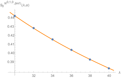
Figure 9: Blue dots represent the numerical values of $S_{0}^{N^{0,1,0},\text{(lmf)}}(\lambda,\alpha)$ and the orange line corresponds to the fitting curve in (193) for Data I (192a).

This concludes that the numerical Data I is consistent with the planar free energy (128). We have also investigated numerical Data II (192b) following the procedure for the $V^{5,2}$ theory described in Appendix C.2, and confirmed that the results again support the planar free energy (128).

References

- (1) J. M. Maldacena, The Large N limit of superconformal field theories and supergravity, Adv. Theor. Math. Phys. 2 (1998) 231–252, [hep-th/9711200].
- (2) E. Witten, Anti-de Sitter space and holography, Adv. Theor. Math. Phys. 2 (1998) 253–291, [hep-th/9802150].
- (3) V. Pestun, Localization of gauge theory on a four-sphere and supersymmetric Wilson loops, Commun. Math. Phys. 313 (2012) 71–129, [0712.2824].
- (4) D. L. Jafferis, I. R. Klebanov, S. S. Pufu and B. R. Safdi, Towards the F-Theorem: N=2 Field Theories on the Three-Sphere, JHEP 06 (2011) 102, [1103.1181].
- (5) H. Casini, M. Huerta and R. C. Myers, Towards a derivation of holographic entanglement entropy, JHEP 05 (2011) 036, [1102.0440].
- (6) H. Casini and M. Huerta, On the RG running of the entanglement entropy of a circle, Phys. Rev. D 85 (2012) 125016, [1202.5650].
- (7) A. Kapustin, B. Willett and I. Yaakov, Exact Results for Wilson Loops in Superconformal Chern-Simons Theories with Matter, JHEP 03 (2010) 089, [0909.4559].
- (8) A. Kapustin, B. Willett and I. Yaakov, Nonperturbative Tests of Three-Dimensional Dualities, JHEP 10 (2010) 013, [1003.5694].
- (9) C. P. Herzog, I. R. Klebanov, S. S. Pufu and T. Tesileanu, Multi-Matrix Models and Tri-Sasaki Einstein Spaces, Phys. Rev. D 83 (2011) 046001, [1011.5487].
- (10) R. C. Santamaria, M. Marino and P. Putrov, Unquenched flavor and tropical geometry in strongly coupled Chern-Simons-matter theories, JHEP 10 (2011) 139, [1011.6281].
- (11) D. L. Jafferis, The Exact Superconformal R-Symmetry Extremizes Z, JHEP 05 (2012) 159, [1012.3210].
- (12) D. Martelli and J. Sparks, The large N limit of quiver matrix models and Sasaki-Einstein manifolds, Phys. Rev. D 84 (2011) 046008, [1102.5289].
- (13) S. Cheon, H. Kim and N. Kim, Calculating the partition function of N=2 Gauge theories on and AdS/CFT correspondence, JHEP 05 (2011) 134, [1102.5565].
- (14) O. Aharony, O. Bergman, D. L. Jafferis and J. Maldacena, N=6 superconformal Chern-Simons-matter theories, M2-branes and their gravity duals, JHEP 10 (2008) 091, [0806.1218].
- (15) N. Drukker, M. Marino and P. Putrov, From weak to strong coupling in ABJM theory, Commun. Math. Phys. 306 (2011) 511–563, [1007.3837].
- (16) D. Z. Freedman and S. S. Pufu, The holography of -maximization, JHEP 03 (2014) 135, [1302.7310].
- (17) D. Gaiotto and A. Tomasiello, The gauge dual of Romans mass, JHEP 01 (2010) 015, [0901.0969].
- (18) T. Suyama, On Large N Solution of Gaiotto-Tomasiello Theory, JHEP 10 (2010) 101, [1008.3950].
- (19) T. Suyama, A Systematic Study on Matrix Models for Chern-Simons-matter Theories, Nucl. Phys. B 874 (2013) 528–566, [1304.7831].
- (20) M. Marino and P. Putrov, ABJM theory as a Fermi gas, J. Stat. Mech. 1203 (2012) P03001, [1110.4066].
- (21) A. Guarino, D. L. Jafferis and O. Varela, String Theory Origin of Dyonic N=8 Supergravity and Its Chern-Simons Duals, Phys. Rev. Lett. 115 (2015) 091601, [1504.08009].
- (22) H. Fuji, S. Hirano and S. Moriyama, Summing Up All Genus Free Energy of ABJM Matrix Model, JHEP 08 (2011) 001, [1106.4631].
- (23) T. Nosaka, Instanton effects in ABJM theory with general R-charge assignments, JHEP 03 (2016) 059, [1512.02862].
- (24) M. Mezei and S. S. Pufu, Three-sphere free energy for classical gauge groups, JHEP 02 (2014) 037, [1312.0920].
- (25) A. Grassi and M. Marino, M-theoretic matrix models, JHEP 02 (2015) 115, [1403.4276].
- (26) Y. Hatsuda and T. Okazaki, Fermi-gas correlators of ADHM theory and triality symmetry, SciPost Phys. 12 (2022) 005, [2107.01924].
- (27) S. M. Chester, S. S. Pufu, Y. Wang and X. Yin, Bootstrapping M-theory Orbifolds, 2312.13112.
- (28) I. R. Klebanov and A. A. Tseytlin, Entropy of near extremal black p-branes, Nucl. Phys. B 475 (1996) 164–178, [hep-th/9604089].
- (29) N. Bobev, A. M. Charles, K. Hristov and V. Reys, The Unreasonable Effectiveness of Higher-Derivative Supergravity in AdS4 Holography, Phys. Rev. Lett. 125 (2020) 131601, [2006.09390].
- (30) N. Bobev, A. M. Charles, K. Hristov and V. Reys, Higher-derivative supergravity, AdS4 holography, and black holes, JHEP 08 (2021) 173, [2106.04581].
- (31) S. Bhattacharyya, A. Grassi, M. Marino and A. Sen, A One-Loop Test of Quantum Supergravity, Class. Quant. Grav. 31 (2014) 015012, [1210.6057].
- (32) N. Bobev, J. Hong and V. Reys, Large N Partition Functions, Holography, and Black Holes, Phys. Rev. Lett. 129 (2022) 041602, [2203.14981].
- (33) N. Bobev, J. Hong and V. Reys, Large N partition functions of the ABJM theory, JHEP 02 (2023) 020, [2210.09318].
- (34) K. Hristov, ABJM at finite N via 4d supergravity, JHEP 10 (2022) 190, [2204.02992].
- (35) S. Geukens and N. Bobev, Supersymmetric Localization: A study of strongly interacting QFTs with applications to Quantum Gravity, Master’s thesis, KU Leuven, 2023.
- (36) N. Hama, K. Hosomichi and S. Lee, Notes on SUSY Gauge Theories on Three-Sphere, JHEP 03 (2011) 127, [1012.3512].
- (37) S. M. Hosseini and N. Mekareeya, Large topologically twisted index: necklace quivers, dualities, and Sasaki-Einstein spaces, JHEP 08 (2016) 089, [1604.03397].
- (38) N. Bobev, J. Hong and V. Reys, Large N partition functions of 3d holographic SCFTs, JHEP 08 (2023) 119, [2304.01734].
- (39) D. L. Jafferis, Quantum corrections to Chern-Simons theories with flavor and their AdS4 duals, JHEP 08 (2013) 046, [0911.4324].
- (40) D. Martelli and J. Sparks, AdS(40 / CFT(3) duals from M2-branes at hypersurface singularities and their deformations, JHEP 12 (2009) 017, [0909.2036].
- (41) D. Gaiotto and D. L. Jafferis, Notes on adding D6 branes wrapping RP**3 in AdS(4) x CP**3, JHEP 11 (2012) 015, [0903.2175].
- (42) S. Hohenegger and I. Kirsch, A Note on the holography of Chern-Simons matter theories with flavour, JHEP 04 (2009) 129, [0903.1730].
- (43) Y. Hikida, W. Li and T. Takayanagi, ABJM with Flavors and FQHE, JHEP 07 (2009) 065, [0903.2194].
- (44) S. Cheon, D. Gang, S. Kim and J. Park, Refined test of AdS4/CFT3 correspondence for N=2,3 theories, JHEP 05 (2011) 027, [1102.4273].
- (45) F. Benini, C. Closset and S. Cremonesi, Chiral flavors and M2-branes at toric CY4 singularities, JHEP 02 (2010) 036, [0911.4127].
- (46) S. Cremonesi, Type IIB construction of flavoured ABJ(M) and fractional M2 branes, JHEP 01 (2011) 076, [1007.4562].
- (47) S. Franco, A. Hanany, J. Park and D. Rodriguez-Gomez, Towards M2-brane Theories for Generic Toric Singularities, JHEP 12 (2008) 110, [0809.3237].
- (48) S. Franco, I. R. Klebanov and D. Rodriguez-Gomez, M2-branes on Orbifolds of the Cone over Q**1,1,1, JHEP 08 (2009) 033, [0903.3231].
- (49) B. E. W. Nilsson and C. N. Pope, Hopf Fibration of Eleven-dimensional Supergravity, Class. Quant. Grav. 1 (1984) 499.
- (50) M. Marino, Lectures on localization and matrix models in supersymmetric Chern-Simons-matter theories, J. Phys. A 44 (2011) 463001, [1104.0783].
- (51) J. T. Liu and Y. Lu, Subleading corrections to the free energy in a theory with scaling, JHEP 10 (2020) 169, [1912.04722].
- (52) J. Hong and J. T. Liu, Subleading corrections to the S3 free energy of necklace quiver theories dual to massive IIA, JHEP 11 (2021) 183, [2103.17033].
- (53) J. T. Liu, L. A. Pando Zayas, V. Rathee and W. Zhao, Toward Microstate Counting Beyond Large N in Localization and the Dual One-loop Quantum Supergravity, JHEP 01 (2018) 026, [1707.04197].
- (54) L. A. Pando Zayas and Y. Xin, Universal logarithmic behavior in microstate counting and the dual one-loop entropy of black holes, Phys. Rev. D 103 (2021) 026003, [2008.03239].
- (55) L. A. Pando Zayas and Y. Xin, Topologically twisted index in the ’t Hooft limit and the dual AdS4 black hole entropy, Phys. Rev. D 100 (2019) 126019, [1908.01194].
- (56) Y. Hatsuda and K. Okuyama, Probing non-perturbative effects in M-theory, JHEP 10 (2014) 158, [1407.3786].
- (57) M. Marino, Localization at large N in Chern–Simons-matter theories, J. Phys. A 50 (2017) 443007, [1608.02959].
- (58) S. M. Chester, R. R. Kalloor and A. Sharon, Squashing, Mass, and Holography for 3d Sphere Free Energy, JHEP 04 (2021) 244, [2102.05643].
- (59) A. Cagnazzo, D. Sorokin and L. Wulff, String instanton in AdS(4) x CP**3, JHEP 05 (2010) 009, [0911.5228].
- (60) Y. Hatsuda, S. Moriyama and K. Okuyama, Instanton Effects in ABJM Theory from Fermi Gas Approach, JHEP 01 (2013) 158, [1211.1251].
- (61) F. F. Gautason, V. G. M. Puletti and J. van Muiden, Quantized strings and instantons in holography, JHEP 08 (2023) 218, [2304.12340].
- (62) M. Beccaria, S. Giombi and A. A. Tseytlin, Instanton contributions to the ABJM free energy from quantum M2 branes, JHEP 10 (2023) 029, [2307.14112].
- (63) T. Nosaka, Large N expansion of mass deformed ABJM matrix model: M2-instanton condensation and beyond, 2401.11484.
- (64) J. Minahan, U. Naseer and C. Thull, Squashing and supersymmetry enhancement in three dimensions, SciPost Phys. 12 (2022) 025, [2107.07151].
- (65) S. M. Chester, R. R. Kalloor and A. Sharon, 3d = 4 OPE coefficients from Fermi gas, JHEP 07 (2020) 041, [2004.13603].
- (66) N. Bobev, S. Choi, J. Hong and V. Reys, Large N superconformal indices for 3d holographic SCFTs, JHEP 02 (2023) 027, [2210.15326].
- (67) N. Bobev, S. Choi, J. Hong and V. Reys, Superconformal Indices of 3d holographic SCFTs, to appear (2024) , [xxxx.xxxxx].
- (68) N. Bobev, P.-J. De Smet, J. Hong, V. Reys and X. Zhang, Squashed 3-sphere partition functions and Airy formulae, to appear (2024) , [xxxx.xxxxx].
- (69) J. Ambjørn, L. Chekhov, C. F. Kristjansen and Y. Makeenko, Matrix model calculations beyond the spherical limit, Nucl. Phys. B 404 (1993) 127–172, [hep-th/9302014].
- (70) P. Di Francesco, P. H. Ginsparg and J. Zinn-Justin, 2-D Gravity and random matrices, Phys. Rept. 254 (1995) 1–133, [hep-th/9306153].
- (71) G. Akemann, Higher genus correlators for the Hermitian matrix model with multiple cuts, Nucl. Phys. B 482 (1996) 403–430, [hep-th/9606004].
- (72) R. Dijkgraaf and C. Vafa, Matrix models, topological strings, and supersymmetric gauge theories, Nucl. Phys. B 644 (2002) 3–20, [hep-th/0206255].
- (73) M. Aganagic, A. Klemm, M. Marino and C. Vafa, Matrix model as a mirror of Chern-Simons theory, JHEP 02 (2004) 010, [hep-th/0211098].
- (74) S. K. Ashok, R. Corrado, N. Halmagyi, K. D. Kennaway and C. Romelsberger, Unoriented strings, loop equations, and N = 1 superpotentials from matrix models, Phys. Rev. D 67 (2003) 086004, [hep-th/0211291].
- (75) N. Halmagyi and V. Yasnov, The Spectral curve of the lens space matrix model, JHEP 11 (2009) 104, [hep-th/0311117].
- (76) J. T. Liu and X. Zhang, The large- partition function for non-parity-invariant Chern-Simons-matter theories, JHEP 12 (2020) 007, [2008.09642].
- (77) N. Bobev, M. David, J. Hong, V. Reys and X. Zhang, A compendium of logarithmic corrections in AdS/CFT, JHEP 04 (2024) 020, [2312.08909].
- (78) E. Witten, Chern-Simons gauge theory as a string theory, Prog. Math. 133 (1995) 637–678, [hep-th/9207094].
- (79) R. Gopakumar and C. Vafa, On the gauge theory / geometry correspondence, Adv. Theor. Math. Phys. 3 (1999) 1415–1443, [hep-th/9811131].
- (80) H. Ooguri and C. Vafa, World sheet derivation of a large N duality, Nucl. Phys. B 641 (2002) 3–34, [hep-th/0205297].
- (81) M. Bershadsky, S. Cecotti, H. Ooguri and C. Vafa, Kodaira-Spencer theory of gravity and exact results for quantum string amplitudes, Commun. Math. Phys. 165 (1994) 311–428, [hep-th/9309140].
- (82) B. Eynard, M. Marino and N. Orantin, Holomorphic anomaly and matrix models, JHEP 06 (2007) 058, [hep-th/0702110].
- (83) M. Marino and P. Putrov, Exact Results in ABJM Theory from Topological Strings, JHEP 06 (2010) 011, [0912.3074].
- (84) T. Nosaka, K. Shimizu and S. Terashima, Large N behavior of mass deformed ABJM theory, JHEP 03 (2016) 063, [1512.00249].
- (85) T. Nosaka, K. Shimizu and S. Terashima, Mass Deformed ABJM Theory on Three Sphere in Large N limit, JHEP 03 (2017) 121, [1608.02654].
- (86) J. T. Liu and R. J. Saskowski, Subleading corrections in = 3 Gaiotto-Tomasiello theory, JHEP 08 (2021) 126, [2106.03901].
- (87) N. Hama, K. Hosomichi and S. Lee, SUSY Gauge Theories on Squashed Three-Spheres, JHEP 05 (2011) 014, [1102.4716].
- (88) Y. Imamura and D. Yokoyama, N=2 supersymmetric theories on squashed three-sphere, Phys. Rev. D 85 (2012) 025015, [1109.4734].
- (89) T. W. Grimm, K. Mayer and M. Weissenbacher, Higher derivatives in Type II and M-theory on Calabi-Yau threefolds, JHEP 02 (2018) 127, [1702.08404].
- (90) M. Ozkan, Y. Pang and E. Sezgin, Higher Derivative Supergravities in Diverse Dimensions, 2401.08945.
- (91) S. A. Kurlyand and A. A. Tseytlin, Type IIB supergravity action on M5×X5 solutions, Phys. Rev. D 106 (2022) 086017, [2206.14522].
- (92) M. Beccaria and A. A. Tseytlin, Comments on ABJM free energy on S3 at large N and perturbative expansions in M-theory and string theory, Nucl. Phys. B 994 (2023) 116286, [2306.02862].
- (93) D. J. Gross and E. Witten, Superstring Modifications of Einstein’s Equations, Nucl. Phys. B 277 (1986) 1.