Cross-modality Matching and Prediction of Perturbation Responses with
Labeled Gromov-Wasserstein Optimal Transport

Abstract

It is now possible to conduct large scale perturbation screens with complex readout modalities, such as different molecular profiles or high content cell images. While these open the way for systematic dissection of causal cell circuits, integrated such data across screens to maximize our ability to predict circuits poses substantial computational challenges, which have not been addressed. Here, we extend two Gromov-Wasserstein Optimal Transport methods to incorporate the perturbation label for cross-modality alignment. The obtained alignment is then employed to train a predictive model that estimates cellular responses to perturbations observed with only one measurement modality. We validate our method for the tasks of cross-modality alignment and cross-modality prediction in a recent multi-modal single-cell perturbation dataset. Our approach opens the way to unified causal models of cell biology.

1 Introduction

High-throughput high-content perturbation screens are revolutionizing our ability to interrogate gene function and identify the targets of small molecules (Bock et al., 2022). Advances over the past decade now allow us to efficiently measure the responses of individual cells to tens of thousands of perturbations in terms of different molecular profiles, such as RNA (Dixit et al., 2016), chromatin and/or proteins (Frangieh et al., 2021) (Perturb-Seq) or high content microscopy images (Feldman et al., 2019) (Optical Pooled Screens (OPS)). Because these modalities provide complementary information about how cells respond to perturbation, leveraging multi-modal data with adequate computational methods presents a remarkable opportunity to learn of all aspects of cell biology. First, relating rich molecular profile to cell biology morphological phenotypes helps understand how different levels of organization relate to each other in the cell, a fundamental question in biology. Second, cross-modality translation methods could help reduce experimental costs and speed up discovery. In particular, molecular profiling (Perturb-Seq) screens are usually substantially more costly and less scalable than optical pooled screens, but provide far more mechanistically interpretable results. Predicting molecular profiles (e.g., RNA profiles) from morphological profiling data would thus offer both scalability and interpretability and accelerate discovery.

Cross-modality alignment and prediction are well-studied tasks in (non-perturbational) single-cell genomics. Multiple approaches based on autoencoders (Ashuach et al., 2023) and Gromov-Wasserstein Optimal Transport (GWOT) (Demetci et al., 2022a, b) have successfully tackled these problems for datasets where cell states are clearly demarcated (e.g., discrete cell types). However, data from single-cell perturbation studies are significantly more challenging, because screens are usually conducted in one, relatively homogeneous, cell type, and each perturbation typically only induces a relatively modest change in the cell’s overall state. In such cases, existing alignment methods may perform poorly.

To tackle this, we propose to leverage the perturbation label for each cell, readily available for such data, to infer a more accurate cross-modality alignment. The naive approach of aligning cells across modalities for each perturbation separately is sub-optimal, because multiple different perturbation can cause similar phenotypic shifts (Dixit et al., 2016; Frangieh et al., 2021; Geiger-Schuller et al., 2023), such that samples from other perturbations should provide information about the global topology of the phenotypic space. Instead, we incorporate the label information when learning a model across all the perturbations, and show this substantially improves the performance. Specifically, we adapt GWOT methods, including entropic GWOT  (Peyré et al., 2016) and Co-Optimal Transport (COOT,  Redko et al. (2020)) to exploit this information as a constraint on the learned cross-modality cellular coupling matrix. We then employ the learned coupling matrix to train a cross-modality prediction model (Figure 1) and apply it to estimate the response to perturbations observed only in one modality (out-of-sample). We validate our method by benchmarking against baselines in recent data from a multi-modal small molecule screen.

Figure 1: Schematic of the workflow

2 Related Work

Gromov-Wasserstein Optimal Transport

Let us consider two discrete measures $\mu=\sum_{i=1}^{n}{p_{i}\delta_{x_{i}}}$, and $\nu=\sum_{j=1}^{m}{q_{j}\delta_{y_{j}}}$ with supports $\mathcal{X}$ and $\mathcal{Y}$, respectively. For the cost function $c:\mathcal{X}\times\mathcal{Y}\rightarrow\mathbb{R}_{+}$, the Optimal Transport (OT) problem consists of finding the transport plan (or coupling) $T^{*}\in\mathcal{C}_{p,q}=\{T\in\mathbb{R}_{+}^{n\times m}\mid T\mathds{1}=p,T^{\top}\mathds{1}=q\}$ that minimizes the cost of transporting $\mu$ onto $\nu$  (Monge, 1781; Kantorovich, 1960):

$$\mathcal{OT}(\mu,\nu)=\min_{T\in\mathcal{C}_{p,q}}\sum_{i,j}{c(x_{i},y_{j})T_{ij}}.$$

The cost function is easily defined when both $\mathcal{X}$ and $\mathcal{Y}$ are subsets of a normed vector space (e.g., $c$ is the distance induced by the norm). For multi-modal alignment, however, $\mathcal{X}$ and $\mathcal{Y}$ belong to incomparable spaces. In this scenario, it is more relevant to consider the Gromov-Wasserstein Optimal Transport (GWOT) distance $\mathcal{GW}(\mu,\nu)$, which employs as its cost function the distance between distances (Mémoli, 2011; Alvarez-Melis & Jaakkola, 2018): []

$$\min_{T\in\mathcal{C}_{p,q}}{\sum_{i,j,k,l}d\left(c_{\mathcal{X}}(x_{i},x_{k}),c_{\mathcal{Y}}(y_{j},y_{l})\right)T_{ij}T_{kl}}.$$ (GWOT)

with within-domain cost functions $c_{\mathcal{X}}:\mathcal{X}\times\mathcal{X}\rightarrow\mathbb{R}$, $c_{\mathcal{Y}}:\mathcal{Y}\times\mathcal{Y}\rightarrow\mathbb{R}$ and the cost between costs $d:\mathbb{R}\times\mathbb{R}\rightarrow\mathbb{R}_{+}$.

One important consideration in estimating OT-based distances is the computational burden. Cuturi (2013) showed that adding the entropy of the coupling as a regularization term to the objective function of the OT problem not only yields accurate approximations of OT distances but also significantly enhances computational efficiency. Indeed, the entropic-regularized OT (EOT) problem can be solved with a linear convergence rate algorithm, making it efficient for large-scale problems. Follow-up work from Peyré et al. (2016) showed that entropic-regularized GWOT (EGWOT) reduces to the problem of solving a sequence of EOT problems, and lowered the time for calculating the GW cost for a fixed coupling from $O(n^{2}m^{2})$ to $O(n^{2}m+m^{2}n)$ for certain cost functions, including the $L^{2}$ distance.

COOT (Redko et al., 2020) is an alternative formulation of the GWOT problem, jointly optimizing the transport of the sample measure $\mu$ onto $\nu$ via coupling $T^{s}$, and the transport of the feature measures $\beta=\sum_{k=1}^{d_{1}}r_{k}\delta_{v_{k}},\omega=\sum_{l=1}^{d_{2}}t_{l}\delta_{w_{l}}$, via coupling $T^{v}$. It is defined as: []

$$\min_{\begin{subarray}{c}T^{s}\in\mathcal{C}_{p,q}\\ T^{v}\in\mathcal{C}_{r,t}\end{subarray}}\sum_{i,j,k,l}c(x_{ik},y_{jl})T^{v}_{kl}T^{s}_{ij},$$ (COOT)

where $x_{ik}$ and $y_{jl}$ denote the $k$-th and $l$-th feature of the $i$-th sample $x_{i}$ and the $j$-th sample $y_{j}$, respectively.

EOT, EGWOT, and entropic-regularized COOT (ECOOT) have been applied to single-cell perturbation response prediction (Bunne et al., 2023) and multiomic integration problems (Demetci et al., 2022a, b). However, none of these methods as currently formulated can leverage additional labels for inference of optimal couplings.

Optimal Transport with Additional Structure

Several works studied the OT problem with additional constraints on the coupling. Structured OT (Alvarez-Melis et al., 2018) considered the problem where labeled source samples are transported to unlabeled target samples. Alvarez-Melis & Fusi (2020) studied the OT problem where source and target samples are independently labeled, and calculated the pairwise distances between the source labels and target labels to improve the coupling between the samples. InfoOT (Chuang et al., 2023) promotes the conservation of structure between the source and target space by maximizing the mutual information of the coupling matrix (treated as a joint distribution). HHOT (Yeaton et al., 2022) tackles a hierarchical OT problem, where samples’ Wasserstein distances are used as the cost to calculate the sample-group-level Wasserstein distances. While these studies solved variants of the OT problem that admit sample labels, they do not apply to matching across different spaces.

Domain Adaptation via Representation Matching

Domain adaptation techniques are crucial for overcoming discrepancies between different data distributions. The framework of domain-adversarial neural network (DANN) (Ganin et al., 2016) included an adversarial domain classifier to achieve better generalization to unseen data. DANNs have been applied on latent spaces of auto-encoders for single-cell modality integration tasks (Lopez et al., 2019), as well as histology and RNA-seq data integration (Comiter et al., 2023). Gossi et al. (2023) estimates OT couplings between latent embeddings of two modalities of single-cell data, by constraining OT for label-matched data. Although closest to our problem, those methods require a ground truth matching between samples for training. JDOT (Courty et al., 2017) learns the domain-adaptated classifier $f:\mathcal{X}\rightarrow\mathcal{Y}$ by minimizing OT between sample and label pairs of source and target domains $(X_{s},Y_{s})$ and $(X_{t},f(X_{t}))$. DeepJDOT (Damodaran et al., 2018) extends JDOT to learn a classifier for the target domain given a label only available in the source domain, where the training involves OT coupling of latent target and source samples. While these methods are designed for cross-modality prediction, they do not utilize group-level source and target sample matching.

3 Method

In perturbation data, we observe labels $l^{x}=\{l^{x}_{1},\ldots,l^{x}_{n}\}$ and $l^{y}=\{l^{y}_{1},\ldots,l^{y}_{m}\}$ from modalities $\mathcal{X}$ and $\mathcal{Y}$, respectively. Each individual label $l^{x}_{i}$ and $l^{y}_{j}$ encodes a perturbation in $\{1,\ldots,L\}$, with $L$ the total number of perturbations. As noted above, GWOT and COOT are suitable computational frameworks for aligning data across modalities but are not designed to leverage labels from perturbation data. Application GWOT / COOT as-is to our data would mean either learning a global model but ignoring labels altogether, or learning a separate model per label and losing information about the global topology of the phenotypic space. We thus aimed to generalize both the GWOT and COOT problem formulations to incorporate label information.

3.1 Labeled Entropic-regularized GWOT

Let $B^{l}$ be the label-identity matrix defined as $B^{l}_{ij}:=\mathds{1}\{l^{x}_{i}=l^{y}_{j}\}$. We say a coupling $T\in\mathcal{C}_{p,q}$ is $l$-compatible if for all indices $i,j$, we have that $T_{ij}>0\implies B^{l}_{ij}=1$, and denote as $\mathcal{C}_{p,q}^{l}$ the subset of couplings in $\mathcal{C}_{p,q}$ which are $l$-compatible. The Labeled EGWOT problem is defined as the EGWOT problem with the additional constraint that $T\in\mathcal{C}_{p,q}^{l}$. We first characterize the structure of the solution of the (simpler) EOT problem with the additional label constraint:

Lemma 3.1.

For a label-identity matrix $B^{l}$, the $l$-compatible entropic optimal transport plan

$$\mathcal{T}_{\epsilon}^{l}(c,p,q)=\operatorname*{arg\,min}_{T\in\mathcal{C}^{l}_{p,q}}\langle c,T\rangle-\epsilon H(T),$$ (1)

can be expressed as $\textrm{diag}(u)(e^{-c/\epsilon}\odot B^{l})\textrm{diag}(v)$, where $\odot$ denotes element-wise multiplication.

The proof appears in Appendix A. This result is important, as it entails that the Labeled EOT problem can be efficiently solved with the celebrated Sinkhorn iterations. Next, we note that the reduction of the EGWOT problem to an iterative EOT problem, as described in Peyré et al. (2016), still holds with the additional constraint of $l$-compatible couplings. Therefore, we have the following corollary:

Corollary 3.2.

For a label-identity matrix $B^{l}$, the Labeled EGWOT problem can be solved by the iterative update of $T$ with $T^{k+1}\leftarrow\mathcal{T}_{\epsilon}^{l}(c(c_{\mathcal{X}},c_{\mathcal{Y}})\odot T^{k},p,q)$.

Additionally, we show that if the cost function $d$ satisfies the condition of Proposition 1 from Peyré et al. (2016) (e.g., $d$ is the $L^{2}$ distance), then the cost calculation for any $l$-compatible coupling is accelerated by a factor of $L$ (Appendix B). This is advantageous, as a large screen dataset may be comprised of thousands of perturbations. A complete description of the algorithm appears in Appendix C. We implemented it as an extension of Python library ‘ott-jax‘ (Cuturi et al., 2022).

3.2 Labeled COOT

We adapted Algorithm 1 of Redko et al. (2020) for Labeled COOT and ECOOT by updating each of the $L$ per-label sample transports and a shared global feature transport per iteration (see Appendix D).

Table 1: Evaluation metrics of OT and GW approaches for sample matching, prediction, and feature matching tasks.

		Matching			Prediction						Feature
Method		Bary FOSCTTM ($\downarrow$)	Dosage match ($\uparrow$)	Mean rank	$R_{v}$ ($\uparrow$)	$\rho_{v}$ ($\uparrow$)	$R_{s}$ ($\uparrow$)	$\rho_{s}$ ($\uparrow$)	MSE ($\downarrow$)	Mean rank	Enrich- ment($\uparrow$)
Perfect		0	1	-	0.107	0.118	0.163	0.149	0.258	-	6.95
By dosage		0.239	1	-	0.0812	0.0448	0.0903	0.0863	0.264	-	5.16
Uniform per label		0.298	0.357	-	0.0794	0.0403	0.0761	0.0781	0.264	-	1.85
EOT	no label	0.428	0.040	9	0.0482	0.007	0.0068	0.0063	0.287	7	1.10
	per label	0.336	0.346	5	0.0544	0.0239	0.0345	0.0307	0.283	5.2	1.26
ECOOT	no label	0.414	0.049	8	0.053	0.0207	0.0395	0.0408	0.282	5	1.07
	labeled	0.270	0.456	2	0.0852	0.0523	0.0854	0.0778	0.265	1.6	5.31
EGWOT	no label	0.373	0.068	7	0.0631	0.0227	0.0302	0.034	0.282	4.8	3.74
	per label	0.332	0.381	4	0.0785	0.0449	0.0737	0.0737	0.265	2.6	1.26
	labeled	0.283	0.452	3	0.0836	0.044	0.0854	0.0825	0.264	1.8	19.8
DAVAE	no label	0.231	0.206	3	0.0342	-0.0069	0.0006	-0.0001	0.33	8	-
	labeled	0.242	0.205	4	0.0182	-0.0079	-0.0016	-0.0014	0.332	9	-

4 Experiments

We tested whether we could (1) match samples across modalities so that similar samples are matched with each other and (2) predict the response to perturbations in one modality given the response to that perturbation measured in the other modality. We further (3) learned feature matching by plugging the learned sample matching $T_{s}$ into ECOOT and solving the OT problem. Full experimental details appear in Appendix E.

Data

The dataset records single-cell RNA (2000 genes) and protein (123 proteins) profiles of T cells undergoing TCR activation following perturbation with kinase inhibitors. The dataset includes 11 inhibitors, used at varying concentrations (100 nM, 1 µM, and 10 µM), as well as negative controls (vehicle and non-activation). We normalized and scaled features following conventional single-cell data processing pipelines and used the first 50 principal components of each modality as the input for OT-based methods.

Methods

We compared labeled ECOOT and EGWOT against the baseline of EOT, ECOOT, and EGWOT without sample labels (no label), and per label EOT and EGWOT. For the prediction task, we trained a multilayer perceptron (MLP) to predict RNA levels from protein measurements according to the learned coupling $T$. Specifically, for training, a sample from the RNA modality $y_{j}$ is randomly sampled for each sample from the protein modality $x_{i}$ as $j\sim\text{Multinomial}(T_{i\cdot}/\sum T_{i\cdot})$, independently for each minibatch. For the matching and prediction task, we included additional baselines of domain-adversarial VAE (DAVAE) and its naive label adaptation described in Appendix F.

Evaluation

We evaluated the matching for the observed treatments and assessed the prediction for the held-out treatments. Because the data were collected using a mult-modal profiling method (where RNA and protein profiles are measured jointly for each single cell), we have a ground-truth cell-to-cell matching from the data. Thus, for the matching, we calculated the barycentric FOSCTTM (Liu et al., 2019), the fraction of the barycentric projections closer than the true match (as in Demetci et al. (2022a)). We further evaluated the matching in treated cells, using the ground-truth RNA profiles ($\{d^{x}_{1},\ldots,d^{x}_{n}\}$) and protein profiles ($\{d^{y}_{1},\ldots,d^{y}_{m}\}$). Given the treated cell profiles, we expect cells treated with the same dose to match. We thus use the dose labels to evaluate the matching, by taking the sum of the coupling weights $\sum_{ij}T_{ij}$ for the samples with matching doses $(i,j)\in\{i,j\mid l^{x}_{i}=l^{y}_{j}=k,d^{x}_{i}=d^{y}_{j}\}$ and denote it as dosage match. For the prediction task, we calculated the mean Pearson ($R$) and Spearman ($\rho$) correlation coefficients between gene expression fold changes in real vs. predicted profiles, where the fold changes are calculated over the mean expression level of genes in the cells treated by vehicle. This was done for each cell ($R_{v}$, $\rho_{v}$), and between cells for each feature ($R_{s}$, $\rho_{s}$). We also report the mean squared error (MSE) between the predicted and true gene expression profile. For the feature matching, we calculated the enrichment of coupling weights in 23 ground truth protein and RNA matches over the uniform feature coupling (Appendix E).

Hyperparameter selection

We conducted a nested 5-fold cross-validation (CV) by splitting treatments into a train, validation, and test sets. The best hyperparameters for matching and prediction tasks were independently selected from the inner CV. We performed a Hyperparameter search for the entropic regularizer weight $\epsilon\in\{10^{-2},10^{-3},10^{-4},10^{-5}\}$ where the maximum cost was normalized as $1$ for entropic OT and GW methods. COOT methods used the same $\epsilon$ for all sample and feature OTs. The scale of the adversarial loss $\lambda^{Adv}$ was optimized across $\{1,5,10,50,100\}$ for DAVAEs. Hyperparameters with the least barycentric FOSCTTM for the matching and the highest $R_{s}$ for the prediction were independently selected for each outer CV fold. We report the mean evaluation metrics across the outer folds. For feature matching, we obtained the best sample matchings with the highest dosage match among the $\epsilon$ in the same grid to calculate feature matchings across the same $\epsilon$’s and report the best enrichment.

Results

Overall, GWOT-based methods (EGWOT and ECOOT variants) outperformed OT-based methods (Table 1). This highlights the importance of optimizing distance between distances rather than naively assuming the existence of shared cost metric even when the number of the dimensions of the source and target modalities are the same.

DAVAE methods showed poor prediction performance despite decent matching (Table 1). Although we have not investigated the cause, it may be due to the instability of adversarial training (Kodali et al., 2017) and the small hyperparameter search space. A comprehensive hyperparameter search and alternative domain adaptation methods may improve the performance.

Within GWOT-based methods, not using the label information led to poor performance, as they fail to harness the strong matching information provided by the input sample labels. Per-label GWOT-based methods performed better than methods without label input, but did not achieve as high matching and prediction performance as the label-aware GWOT-based methods.

The superior sample matching, prediction, and feature matching performance of labeled GWOT-based methods stems from information sharing across different labels, while still constraining the sample matching by labels. Specifically, when Labeled EGWOT calculates the cost between samples with the same label, it will consider the distance of each sample to the samples with other labels (Appendix B). For Labeled ECOOT, the sample couplings for all labels explicitly share the global coupling between features. We present further results and visualizations in Appendix G.

5 Discussion

We provide a mathematical and algorithmic adaptation of GWOT methods for the case when sample labels are available. These methods outperform OT, GWOT, and DAVAE baselines both in cross-modality matching and prediction tasks. Labeled GWOT-based methods had improved matching between raw features from the sample matching, suggesting their potential to improve the interpretability of features. We note that learning sample matching from the latent representation provides substantial computational acceleration over the learning in the raw feature space.

We expect our framework to combine the modality-specific strengths of different high content perturbation screens, such as the high scalability of optical pooled screens (Feldman et al., 2019) and the high resolution and interpretability of Perturb-seq (Dixit et al., 2016). As GWOT-based methods rely on the sample-to-sample cost within each modality, more sophisticated latent representation may be needed to remove any large modality-specific variations.

Code Availability Statement

We implement our new model and benchmarks using the Python ‘scvi-tools‘  (Gayoso et al., 2022) and ‘ott-jax‘  (Cuturi et al., 2022) libraries, and release it as open-source software at https://genentech.github.io/Perturb-OT/.

Data Availability Statement

Input data used for the experiments in this manuscript are currently undergoing publication as a separate manuscript. They will become publicly available upon acceptance.

Appendices

Appendix A details the proof of Lemma 3.1. Appendix B describes the acceleration of the cost calculation for both unlabeled and labeled GWOT, following the assumptions of Peyré et al. (2016) regarding the decomposition for the cost function. Appendix C describes the algorithm for solving labeled EGWOT problems. Appendix D describes the labeled COOT problem and the algorithm we propose for numerical resolution. In Appendix E, we provide details about data pre-processing, model architecture, as well as training procedures used for the experiments. In F, we describe the naive adaptation of DAVAE to the labeled setting. In Appendix G, we show extended experimental results.

Appendix A Proof of Lemma 3.1

We remind the reader that the label-identity matrix $B^{l}$ is defined as $B^{l}_{ij}=\mathds{1}\{l^{x}_{i}=l^{y}_{j}\}$, where $l^{x}=\{l^{x}_{1},\ldots,l^{x}_{n}\}$ and $l^{y}=\{l^{y}_{1},\ldots,l^{y}_{m}\}$ denotes the perturbation labels from modalities $\mathcal{X}$ and $\mathcal{Y}$, respectively. See 3.1 We note that comparing Lemma 3.1 with Lemma 2 in Cuturi (2013), the solution of $l$-compatible OT is equivalent to the regular EOT with $c(x_{i},y_{j})=+\infty$ for $i,j\in\{(i,j)|l_{x_{i}}\neq l_{y_{j}}\}$. The proof below makes this argument more precise.

Proof.

The $l$-compatible EOT (Labeled EOT) problem is defined as the following optimization problem:

$$\mathcal{OT}_{\epsilon}^{l}(p,q)=\mathop{\min}\limits_{T\in\mathcal{C}_{p,q}^{l}}\langle c,T\rangle-\epsilon H(T)$$ (2)

We may equivalently reformulate the optimization problem using Lagrange multipliers:

$$\mathcal{OT}_{\epsilon}^{l}(p,q) =\min\limits_{T}\max\limits_{\lambda^{p},\lambda^{q},\Lambda^{B}}\langle c,T\rangle-\epsilon H(T)+\langle\lambda^{p},p-T\mathds{1}_{m}\rangle+\langle\lambda^{q},q-T^{\top}\mathds{1}_{n}\rangle+\langle T\odot(\mathds{1}_{n}\mathds{1}_{m}^{\top}-B^{l})),\Lambda^{B}\rangle,$$ (3)

and then use the dual formulation:

$$\mathcal{OT}_{\epsilon}^{l}(p,q) =\max\limits_{\lambda^{p},\lambda^{q},\Lambda^{B}}\min\limits_{T}\langle c,T\rangle-\epsilon H(T)+\langle\lambda^{p},p-T\mathds{1}_{m}\rangle+\langle\lambda^{q},q-T^{\top}\mathds{1}_{n}\rangle+\langle T\odot(\mathds{1}_{n}\mathds{1}_{m}^{\top}-B^{l}),\Lambda^{B}\rangle,$$ (4)

where strong duality is guaranteed since the objective function is convex in $T$ and the constraints are affine. The solution to the inner minimization problem, for fixed $\bm{\Lambda}=\{\lambda^{p},\lambda^{q},\Lambda^{B}\}$ is obtained by finding the critical point:

$$\bar{T}_{ij}(\bm{\Lambda})=\exp\left(\frac{1}{\epsilon}\left(-(1-B^{l}_{ij})\Lambda^{B}_{ij}+\lambda^{p}_{i}+\lambda^{q}_{j}-c_{ij}\right)\right).$$ (5)

Now, we notice that for variable $\bar{T}_{ij}(\bm{\Lambda})$, we have that the regularized cost is derived as:

$$\langle c,\bar{T}\rangle-\epsilon H(\bar{T})=\sum_{ij}{c_{ij}\bar{T}_{ij}}+\epsilon\bar{T}_{ij}(\log\bar{T}_{ij}-1),$$ (6)

which, by injecting the value of $\bar{T}_{ij}(\bm{\Lambda})$ into this expression, we obtain:

$$\langle c,\bar{T}\rangle-\epsilon H(\bar{T})=\sum_{ij}{c_{ij}\bar{T}_{ij}}+\bar{T}_{ij}\left(-(1-B^{l}_{ij})\Lambda^{B}_{ij}+\lambda^{p}_{i}+\lambda^{q}_{j}-c_{ij}-\epsilon\right),$$ (7)

from which, after developing the products and identifying dot products, we finally obtain the simplified expression:

$$\langle c,\bar{T}\rangle-\epsilon H(\bar{T})=-\langle\bar{T}\odot(\mathds{1}_{n}\mathds{1}_{m}^{\top}-B^{l}),\Lambda^{B}\rangle+\langle\lambda^{p},\bar{T}\mathds{1}_{m}\rangle+\langle\lambda^{q},\bar{T}^{\top}\mathds{1}_{n}\rangle-\epsilon\langle\mathds{1}_{n},\bar{T}\mathds{1}_{m}\rangle.$$ (8)

Finally, we may inject this result into the dual formulation from (4) to obtain

$$\mathcal{OT}_{\epsilon}^{l}(p,q) =\max\limits_{\lambda^{p},\lambda^{q},\Lambda^{B}}\langle\lambda^{p},p\rangle+\langle\lambda^{q},q\rangle-\epsilon\langle\mathds{1}_{n},\bar{T}_{ij}(\bm{\Lambda})\mathds{1}_{m}\rangle.$$ (9)

To solve this optimization problem, we first define the objective of (9) as $\mathcal{L}_{\lambda}$.

$$\mathcal{L}_{\lambda}(\bm{\Lambda}):=\langle\lambda^{p},p\rangle+\langle\lambda^{q},q\rangle-\epsilon\sum_{ij}\bar{T}_{ij}(\bm{\Lambda})$$ (10)

We now seek to find a critical point for variable $\Lambda^{B}$ for fixed values of $\lambda_{p}$ and $\lambda_{q}$:

$$\frac{\partial\mathcal{L}_{\lambda}}{\partial\Lambda^{B}_{ij}}={\exp\left(\frac{1}{\epsilon}\left(-(1-B^{l}_{ij})\Lambda^{B}_{ij}+\lambda^{p}_{i}+\lambda^{q}_{j}-c_{ij}\right)\right)}(1-B_{ij}^{l})$$ (11)

We now notice that for any pairs of indices $(i,j)$ such that $B^{l}_{ij}=0$, the partial derivative expressed in (11) is positive for all values of $\bm{\Lambda}$, but vanishes for $\Lambda^{B}_{ij}\rightarrow+\infty$ for any fixed values of $\lambda_{p}$ and $\lambda_{q}$. Then, we notice that for any pairs of indices $(i,j)$ such that $B^{l}_{ij}=1$, (9) is constant with respect to $\Lambda^{B}_{ij}$, therefore, in that case we may pick $\Lambda^{B}_{ij}=0$.

Plugging the optimal values for $\Lambda^{B}_{ij}$ in (9), we obtain

$$\mathcal{OT}_{\epsilon}^{l}(p,q) =\max\limits_{\lambda^{p},\lambda^{q}}\langle\lambda^{p},p\rangle+\langle\lambda^{q},q\rangle+\langle R^{\epsilon}(\lambda^{p},\lambda^{q},c),B^{l}\rangle,$$ (12)

where $[R^{\epsilon}(\lambda^{p},\lambda^{q},c)]_{ij}=\exp(\frac{1}{\epsilon}(\lambda^{p}_{i}+\lambda^{q}_{j}-c_{ij}))$. Defining $({\lambda^{p}}^{*},{\lambda^{q}}^{*})$ as the optimal solution for $\eqref{eq:new_opt}$, we now get the optimal transport plan $T^{*}$ for (4):

$$T_{ij}^{*}({\lambda^{p}}^{*},{\lambda^{q}}^{*}) =\begin{cases}\exp(\frac{1}{\epsilon}({\lambda^{p}_{i}}^{*}+{\lambda^{q}_{j}}^{*}-c_{ij})),&\text{if }B_{ij}=1\\ 0,&\text{otherwise}\end{cases}$$

$$=\textrm{diag}(a)(K\odot B^{l})\textrm{diag}(b)$$

where

$$a_{i}=\exp\left(\frac{{\lambda^{p}_{i}}^{*}}{\epsilon}\right),\ b_{j}=\exp\left(\frac{{\lambda^{q}_{j}}^{*}}{\epsilon}\right),\ K_{ij}=\exp\left(-\frac{c_{ij}}{\epsilon}\right),$$ (13)

which completes the proof. ∎

Additionally, we note that $K\odot B^{l}$ can be the input for the Bregman projections described in Remark 4.8 from Peyré & Cuturi (2018). In such case, the Sinkhorn iterations will converge to the solution of the optimization problem.

Appendix B Cost calculation of labeled GWOT

We present how to speed up the calculation of the cost in the case of labeled GWOT when the cost functions $d$ can be written as

$$d(a,b)=f_{1}(a)+f_{2}(b)-h_{1}(a)h_{2}(b).$$ (14)

This includes a wide array of cost functions, including the $L^{2}$ distance $d(a,b)=\|a\|^{2}+\|b\|^{2}-2\|a\|\|b\|$. For such functions, Peyré et al. (2016) proposed an algorithm to speed up the cost calculations of GWOT. We first present this development, and then show how it can be adapted to the labeled GWOT problem to further improve the speed up.

Recall the cost of GWOT is written as

$$\min_{T\in\mathcal{C}_{p,q}}{\sum_{i,j,k,l}\mathcal{D}_{ijkl}T_{ij}T_{kl}},$$ (15)

where $\mathcal{D}_{ijkl}=c(c_{\mathcal{X}}(x_{i},x_{k}),c_{\mathcal{Y}}(y_{j},y_{l}))$, and $T\in\mathbb{R}^{n\times m}$. With tensor-matrix multiplication $\mathcal{D}\otimes T\in\mathbb{R}^{n\times m}$ defined on 4-dimensional tensor $\mathcal{D}\in\mathbb{R}^{n\times m\times n^{\prime}\times m^{\prime}}$ defined as $[\mathcal{D}\otimes T]_{ij}:=\sum_{k,l}\mathcal{D}_{ijkl}T_{kl},$ the objective function of (15) can be written as $\langle\mathcal{D}\otimes T,T\rangle.$

Peyré et al. (2016) showed that for the cost function $d$ in the form (14), $\mathcal{D}\otimes T$ can be simplified as follows. Let $M_{ij}=c_{\mathcal{X}}(x_{i},x_{j})$ and $\bar{M}_{ij}=c_{\mathcal{Y}}(y_{i},y_{j})$ denote the cost matrices on each modality. Let us define $c_{M,\bar{M}}=f_{1}(M)p\mathds{1}_{m}^{\top}+\mathds{1}_{n}q^{\top}f_{2}(\bar{M})^{\top}$, and notice that

$$\langle\mathcal{D}\otimes T,T\rangle=\langle c_{M,\bar{M}}-h_{1}(M)Th_{2}(\bar{M})^{\top},T\rangle.$$ (16)

Using this formulation, the cost $\mathcal{D}\otimes T$ may be calculated in time $O(n^{2}m+nm^{2})$, instead of $O(n^{2}m^{2})$.

We now show that the calculation of $\mathcal{D}\otimes T$ in (16) can be further accelerated when $T\in\mathcal{C}_{p,q}^{l}$. Let us adopt the notation for the indices of the source and target samples of a given label $k$ as $l_{x}^{\raisebox{0.60275pt}{$\text{-}\scriptscriptstyle\!1$}}(k)=\{i\mid l^{x}_{i}=k\}$ and $l_{y}^{\raisebox{0.60275pt}{$\text{-}\scriptscriptstyle\!1$}}(k)=\{j\mid l^{y}_{j}=k\}$, respectively. In particular, for each label $k$ we denote as $n^{k}=|l_{x}^{\raisebox{0.60275pt}{$\text{-}\scriptscriptstyle\!1$}}(k)|$ and $m^{k}=|l_{y}^{\raisebox{0.60275pt}{$\text{-}\scriptscriptstyle\!1$}}(k)|$ the number of samples with that particular label in modality $\mathcal{X}$ and $\mathcal{Y}$, respectively.

For a matrix $A$, we denote as $[A]_{\{i_{1},\ldots,i_{n}\},\{j_{1},\ldots,j_{m}\}}$ the submatrix of $A$ with $i_{1},\ldots,i_{n}$-th rows and $j_{1},\ldots,j_{m}$-th columns. Several submatrices are now introduced to calculate the optimal transport cost at the resolution of the labels. We denote as $T_{k}\in\mathbb{R}^{n^{k}\times m^{k}}$, the submatrix corresponding to the label-specific coupling:

$$T_{k}\coloneq [T]_{l_{x}^{\raisebox{0.43054pt}{$\text{-}\scriptscriptstyle\!1$}}(k),l_{y}^{\raisebox{0.43054pt}{$\text{-}\scriptscriptstyle\!1$}}(k)}.$$ (17)

Then, for a pair of labels $(k_{1},k_{2})$, we define the submatrices $M^{k_{1}k_{2}}\in\mathbb{R}^{n^{k}_{1}\times n^{k_{2}}}$, $\bar{M}^{k_{1}k_{2}}\in\mathbb{R}^{m^{k}_{1}\times m^{k_{2}}}$ as:

$$M^{k_{1}k_{2}}\coloneq [M]_{l_{x}^{\raisebox{0.43054pt}{$\text{-}\scriptscriptstyle\!1$}}(k_{1}),l_{x}^{\raisebox{0.43054pt}{$\text{-}\scriptscriptstyle\!1$}}(k_{2})}$$ (18)

$$\bar{M}^{k_{1}k_{2}}\coloneq [\bar{M}]_{l_{y}^{\raisebox{0.43054pt}{$\text{-}\scriptscriptstyle\!1$}}(k_{1}),l_{y}^{\raisebox{0.43054pt}{$\text{-}\scriptscriptstyle\!1$}}(k_{2})}.$$ (19)

With the definition, consider calculating (16) for $T\in\mathcal{C}_{p,q}^{l}$. We only need the $(i,j)$-th entries of $\mathcal{D}\otimes T$ for indices $(i,j)$ such that $l^{x}_{i}=l^{y}_{j}$, because any other entry would not contribute to the final cost. We calculate the $[\mathcal{D}\otimes T]_{l_{x}^{\raisebox{0.43054pt}{$\text{-}\scriptscriptstyle\!1$}}(k),l_{y}^{\raisebox{0.43054pt}{$\text{-}\scriptscriptstyle\!1$}}(k)}$ for each label $k$ by calculating each terms of (16) for the label.

$$[c_{M,\bar{M}}]_{ij} =\sum_{i^{\prime}=1}^{n}f_{1}(M_{ii^{\prime}})p_{i^{\prime}}+\sum_{j^{\prime}=1}^{m}f_{2}(\bar{M}_{jj^{\prime}})q_{j^{\prime}}$$

$$=\sum_{k^{\prime}=1}^{L}\left(\sum_{i^{\prime}\in l_{x}^{\raisebox{0.43054pt}{$\text{-}\scriptscriptstyle\!1$}}(k^{\prime})}f_{1}(M_{ii^{\prime}})p_{i^{\prime}}+\sum_{j^{\prime}\in l_{y}^{\raisebox{0.43054pt}{$\text{-}\scriptscriptstyle\!1$}}(k^{\prime})}f_{2}(\bar{M}_{jj^{\prime}})q_{j^{\prime}}\right)$$ (20)

Writing this in a matrix form gives

$$[c_{M,\bar{M}}]_{l_{x}^{\raisebox{0.43054pt}{$\text{-}\scriptscriptstyle\!1$}}(k),l_{y}^{\raisebox{0.43054pt}{$\text{-}\scriptscriptstyle\!1$}}(k)}=\sum_{k^{\prime}=1}^{L}f_{1}(M^{kk^{\prime}})p_{k^{\prime}}+\sum_{k^{\prime}=1}^{L}f_{2}(\bar{M}^{kk^{\prime}})q_{k^{\prime}}$$ (21)

The second term in (16) can be written as

$$[h_{1}(M)Th_{2}(\bar{M})^{\top}]_{ij}=\sum_{i^{\prime}=1}^{n}\sum_{j^{\prime}=1}^{m}h_{1}(M_{ii^{\prime}})T_{i^{\prime}j^{\prime}}h_{2}(\bar{M}_{jj^{\prime}}).$$ (22)

As $T_{i^{\prime}j^{\prime}}=0$ when $l^{x}_{i}\neq l^{y}_{j}$,

$$[h_{1}(M)Th_{2}(\bar{M})^{\top}]_{ij}=\sum_{k=1}^{L}\sum_{i^{\prime}\in\\ l_{x}^{\raisebox{0.43054pt}{$\text{-}\scriptscriptstyle\!1$}}(k)}\sum_{j^{\prime}\in\\ l_{y}^{\raisebox{0.43054pt}{$\text{-}\scriptscriptstyle\!1$}}(k)}h_{1}(M_{ii^{\prime}})T_{i^{\prime}j^{\prime}}h_{2}(\bar{M}_{jj^{\prime}}).$$ (23)

Writing this in a matrix form gives

$$[h_{1}(M)Th_{2}(\bar{M})^{\top}]_{l_{x}^{\raisebox{0.43054pt}{$\text{-}\scriptscriptstyle\!1$}}(k),l_{y}^{\raisebox{0.43054pt}{$\text{-}\scriptscriptstyle\!1$}}(k)}=\sum_{k^{\prime}=1}^{L}h_{1}(M^{kk^{\prime}})T^{kk^{\prime}}h_{2}(\bar{M}^{kk^{\prime}})^{\top}$$ (24)

which shows that the cost calculation of each label $k$ involves the cost between the samples of label $k$ and the samples of all other labels. Combining two terms gives

$$[\mathcal{D}\otimes T]_{l_{x}^{\raisebox{0.43054pt}{$\text{-}\scriptscriptstyle\!1$}}(k),l_{y}^{\raisebox{0.43054pt}{$\text{-}\scriptscriptstyle\!1$}}(k)}=\sum_{k^{\prime}=1}^{L}f_{1}(M^{kk^{\prime}})p_{k^{\prime}}+\sum_{k^{\prime}=1}^{L}f_{1}(\bar{M}^{kk^{\prime}})q_{k^{\prime}}-\sum_{k^{\prime}=1}^{L}h_{1}(M^{kk^{\prime}})T^{kk^{\prime}}h_{2}(\bar{M}^{kk^{\prime}})^{\top}$$ (25)

With balanced number of samples $n^{k}=\frac{n}{L}$, $m^{k}=\frac{m}{L}$, calculating (25) takes $\frac{n^{2}}{L}+\frac{m^{2}}{L}+\frac{n^{2}m}{L^{2}}+\frac{nm^{2}}{L^{2}}$ operations which reduces to $O((n^{2}m+nm^{2})/L^{2})$. Calculating this for all labels gives $\mathcal{D}\otimes T$ with $O((n^{2}m+nm^{2})/L)$ operations, providing $L$ times acceleration compared to the original result from Peyré et al. (2016).

Appendix C Algorithm for solving labeled EGWOT

Given the cost matrices defined in Appendix B, corollary 3.2 provides the following algorithm for labeled EGWOT.

Algorithm 1 Computation of $l$-compatible EGWOT

1:  Input: $M,\bar{M},\epsilon,B^{l},p,q$

2:  Initialize $T$.

3:  repeat

4:     // compute $c_{s}=\mathcal{D}\otimes T$ as in (25).

5:     $c_{s}\leftarrow\mathcal{D}\otimes T$.

6:     // Sinkhorn iterations to compute $\mathcal{T}^{l}_{\epsilon}(c_{s},p,q)$

7:     Initialize $a\leftarrow\mathds{1}$, set $K\leftarrow e^{-c_{s}/\epsilon}\odot B^{l}$.

8:     repeat

9:        $b\leftarrow\frac{q}{K^{\top}a}$, $a\leftarrow\frac{p}{Kb}$

10:     until convergence

11:     Update $T\leftarrow\textrm{diag}(a)(e^{-c_{s}/\epsilon}\odot B^{l})\textrm{diag}(b)$

12:  until convergence

Assuming samples are sorted by their labels, block matrix $K\odot B^{l}$ can further accelerate the calculation of Sinkhorn updates in line 9. As $K_{ij}=0$ when $l^{x}_{i}\neq l^{y}_{j}$, we can write the Sinkhorn update as

$$a_{i} \leftarrow\frac{p_{i}}{\sum_{j=1}^{m}K_{ij}b_{j}}=\frac{p_{i}}{\sum_{j\in\{j|l^{x}_{i}=l^{y}_{j}\}}K_{ij}b_{j}}$$

$$b_{j} \leftarrow\frac{q_{j}}{\sum_{i=1}^{n}K_{ji}a_{i}}=\frac{q_{j}}{\sum_{i\in\{i|l^{x}_{i}=l^{y}_{j}\}}K_{ji}a_{i}}$$

Let $[v]_{\{i_{1},i_{2},\ldots,i_{n}\}}$ denote the smaller vector $(v_{i_{1}},\ldots,v_{i_{n}})$ consisted of the $i_{1},\ldots,i_{n}$-th entries of a vector $v$. The updates can be written in the matrix form for the entries corresponding to a label $k$, where $\varoslash$ denotes the element-wise division.

$$[a]_{l_{x}^{\raisebox{0.43054pt}{$\text{-}\scriptscriptstyle\!1$}}(k)} \leftarrow[p]_{l_{x}^{\raisebox{0.43054pt}{$\text{-}\scriptscriptstyle\!1$}}(k)}\varoslash[K]_{l_{x}^{\raisebox{0.43054pt}{$\text{-}\scriptscriptstyle\!1$}}(k),l_{y}^{\raisebox{0.43054pt}{$\text{-}\scriptscriptstyle\!1$}}(k)}[b]_{l_{y}^{\raisebox{0.43054pt}{$\text{-}\scriptscriptstyle\!1$}}(k)}$$

$$[b]_{l_{y}^{\raisebox{0.43054pt}{$\text{-}\scriptscriptstyle\!1$}}(k)} \leftarrow[q]_{l_{y}^{\raisebox{0.43054pt}{$\text{-}\scriptscriptstyle\!1$}}(k)}\varoslash([K]_{l_{x}^{\raisebox{0.43054pt}{$\text{-}\scriptscriptstyle\!1$}}(k),l_{y}^{\raisebox{0.43054pt}{$\text{-}\scriptscriptstyle\!1$}}(k)})^{\top}[a]_{l_{x}^{\raisebox{0.43054pt}{$\text{-}\scriptscriptstyle\!1$}}(k)}$$

With the balanced number of samples per label $n^{k}=n/L$ and $m^{k}=m/L$, updating for the entries corresponding to a single label is $O(nm/L^{2})$ and the overall update for all labels is $O(nm/L)$, providing $L$ times speedup compared to the Sinkhorn update for $T$ that is not $l$-compatible.

Appendix D Labeled COOT

We adapt COOT to learn a global feature transport plan $T^{v}$ and per-label sample transport plans ${T^{s}}^{(a)}$ for each label $a$. Here we define ${T^{s}}^{(a)}$ as $[T^{s}]_{l_{x}^{\raisebox{0.43054pt}{$\text{-}\scriptscriptstyle\!1$}}(a),l_{y}^{\raisebox{0.43054pt}{$\text{-}\scriptscriptstyle\!1$}}(a)}$ for $l$-compatible $T^{s}$. We note that ${T^{s}}^{(a)}\in\mathcal{C}_{p^{a}q^{a}}$, where $p^{a}=[p]_{l_{x}^{\raisebox{0.43054pt}{$\text{-}\scriptscriptstyle\!1$}}(a)}$, $q^{a}=[q]_{l_{y}^{\raisebox{0.43054pt}{$\text{-}\scriptscriptstyle\!1$}}(a)}$.

Recall that COOT is defined as (COOT) and its entropic-regularized version is written as

$$\min_{\begin{subarray}{c}T^{s}\in\mathcal{C}_{p,q}\\ T^{v}\in\mathcal{C}_{r,t}\end{subarray}}\sum_{i,j,k,l}c(x_{ik},y_{jl})T^{v}_{kl}T^{s}_{ij}-\epsilon^{s}H(T_{s})-\epsilon^{v}H(T_{v}).$$ (ECOOT)

We define the labeled entropy-regularized COOT problem as follows.

$$\min_{T^{v}\in\mathcal{C}_{r,t}}\sum_{k=1}^{L}\min_{{T^{s}}^{(a)}\in\mathcal{C}_{p^{a},q^{a}}}\left(\sum_{\begin{subarray}{c}(i,j)\in\{i,j|l^{x}_{i}=l^{y}_{j}=a\}\\ k,l\end{subarray}}c(x_{ik},y_{jl})T^{v}_{kl}{T^{s}}^{(a)}_{ij}-{\epsilon^{s}}^{(a)}H({T^{s}}^{(a)})\right)-\epsilon^{v}H(T^{v})$$ (Labeled entropic COOT)

The block coordinate descent (BCD) algorithm in Algorithm 1 of Redko et al. (2020) is still valid for the optimization as independent updates of ${T^{s}}^{(1)},\ldots,{T^{s}}^{(L)}$ together are equivalent to a single step of the sample transport update. We adapted the BCD algorithm for labeled COOT as Algorithm 2.

We first define the notations for the algorithm. $X^{a}$ and $Y^{a}$ denote column submatrices $X^{a}=[X]_{\cdot,l_{x}^{\raisebox{0.43054pt}{$\text{-}\scriptscriptstyle\!1$}}(a)}$ and $Y^{a}=[Y]_{\cdot,l_{y}^{\raisebox{0.43054pt}{$\text{-}\scriptscriptstyle\!1$}}(a))}$, $\mathcal{K}$ is a 4-way tensor with elements $\mathcal{K}_{ijkl}=c(x_{ik},y_{jl})$, $\mathcal{K}^{\prime}$ is $\mathcal{K}$ with permuted dimensions with elements $\mathcal{K}^{\prime}_{klij}=c(x_{ik},y_{jl})$ , $\mathcal{K}^{\prime a}$ is a subtensor of $\mathcal{K}^{\prime}$ for samples with label $a$, with elements $\mathcal{K}^{\prime a}_{klij}$ for $(i,j)$ with the same label $l^{x}_{i}=l^{y}_{j}=a$, and $\mathcal{T}_{\epsilon}$ is the entropic OT solution

$$\mathcal{T}_{\epsilon}(p,q,c)=\mathop{\arg\min}\limits_{T\in\mathcal{C}_{p,q}}\langle c,T\rangle-\epsilon H(T).$$

which is obtained by the Sinkhorn algorithm.

Algorithm 2 BCD algorithm for labeled entropic COOT

1:  Input: $X,Y,l,p,q,\epsilon^{v},\epsilon^{s(1)},\ldots,\epsilon^{s(L)}$

2:  Initialize $T^{s(1)}$, …, $T^{s(L)}$, $T^{v}$.

3:  repeat

4:     $T^{v}\leftarrow\mathcal{T}_{\epsilon^{v}}(r,t,\sum_{a=1}^{L}\mathcal{K}^{\prime a}\otimes{T^{s}}^{(a)})$.

5:     for $a=1$ to $L$ do

6:        ${T^{s}}^{(a)}\leftarrow\mathcal{T}_{{\epsilon^{s}}^{(a)}}(p^{a},q^{a},\mathcal{K}\otimes T^{v})$.

7:     end for

8:  until convergence

Line 4 of Algorithm 2 can be obtained from the $T^{v}$ update (26) in Algorithm 1 of Redko et al. (2020).

$$T^{v}\leftarrow\mathcal{T}_{\epsilon^{v}}(r,t,\mathcal{K}^{\prime}\otimes T^{s})$$ (26)

As $T^{s}\in\mathcal{C}_{p,q}^{l}$ and $T^{s}_{ij}=0$ for $(i,j)\notin\{i,j|l^{x}_{i}=l^{y}_{j}\}$,

$$[\mathcal{K}^{\prime}\otimes T^{s}]_{kl}=\sum_{i,j}\mathcal{K}^{\prime}_{klij}T^{s}_{ij}=\sum_{a=1}^{L}\sum_{i\in l_{x}^{\raisebox{0.43054pt}{$\text{-}\scriptscriptstyle\!1$}}(a)}\sum_{j\in l_{y}^{\raisebox{0.43054pt}{$\text{-}\scriptscriptstyle\!1$}}(a)}\mathcal{K}^{\prime}_{klij}T_{ij}=\sum_{a=1}^{L}\mathcal{K}^{\prime a}\otimes{T^{s}}^{(a)}.$$

We note that the unregularized labeled COOT can also be solved simply by updating with unregularized OT solution $\mathcal{T}$. We have adopted the original implementation and implemented the Sinkhorn iterations in OTT (Cuturi et al., 2022).

Appendix E Experimental details

Multi-omics single-cell data processing

Gene expression (RNA) levels from the kinase inhibitor screening data were library size normalized and log transformed as defaults, and the top 2000 highest variable genes were retained using the ‘scanpy‘ Python library(Wolf et al., 2018). Protein features were manually selected by visual inspection of changes across control perturbations, retaining 123 of 277 measured proteins. Protein modality counts were transformed using centered log ratios (CLRs), as explained in Chung et al. (2021). The first 50 PCs were obtained at this step with the ‘sc.tl.pca‘ command from Wolf et al. (2018). 11 kinase inhibitors with large effects on the PCA space across dosages were selected (Figure 2), along with vehicle treatment and non-stimulated T cells as the negative controls.

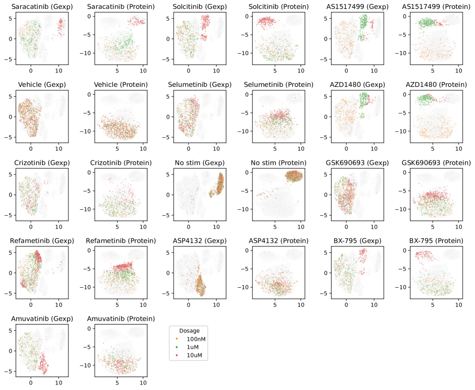
Figure 2: UMAPs of each modality for the cells treated with the selected 13 kinase inhibitors.

Dosage match scores for DAVAEs

Dosage match scores for DAVAEs (see Appendix F) were calculated post-hoc by obtaining coupling from the latent representations. Coupling matrices were obtained by the ‘sc.neighbors._connectivity.gauss‘ command from Wolf et al. (2018) with $k$ across $\{1,5,10,20,30\}$ and the highest dosage match score was reported.

Model structure and training

All OT-based methods were cost-normalized so that the maximum cost is $1$ and allowed for a maximum 2000 iterations both for inner and outer iterations, if applicable. MLPs had 2 hidden layers with 123 dimensions with a batch normalization and ReLU activation layer, followed by a dense linear output layer. Mean squared error is minimized with an Adam optimizer with a learning rate of $10^{-3}$ and early stopping when the validation loss does not decrease for 45 epochs with max 2000 epochs.

Feature matching

We obtained the feature coupling by plugging $T^{s}$ in (ECOOT), resulting in the following EOT problem between features:

$$\min_{T^{v}\in\mathcal{C}_{r,t}}\sum_{i,j,k,l}c(x_{ik},y_{jl})T^{v}_{kl}T^{s}_{ij}-\epsilon^{v}H(T_{v}).$$

We used the 23 proteins/RNAs that were measured in both modalities: CD70, CD52, CD7, TIGIT, CD69, CTLA4, LAG3, CD27, Fas, BTLA, ITGB7, CD83, CXCR4, CD55, CD38, CD9, CD109, CD84, FOXP3, CTLA4, IRF4, GATA3, FOXP3.

Appendix F Labeled domain-adversarial VAE

We have modified MultiVI (Ashuach et al., 2023) to account for labels when calculating adversarial loss. Here, the adversarial classifier accepts the label to promote matching modality per label with the following loss.

$$\mathop{\min}\limits_{\theta,\phi}\max\limits_{\zeta}\mathcal{L}=\mathop{\min}\limits_{\theta,\phi}\max\limits_{\zeta}\mathcal{L}^{\text{ELBO}}_{\theta,\phi}(X,Y)+\lambda\mathcal{L}^{Adv}_{\zeta,\phi}(X,Y,l)$$ (27)

Loss terms of (27) are as follows.

$$\mathcal{L}^{\text{ELBO}}_{\theta,\phi}(X,Y) =-(\text{ELBO}_{\theta_{X},\phi_{X}}(X)+\text{ELBO}_{\theta_{Y},\phi_{Y}}(Y))$$

$$\mathcal{L}^{Adv}_{\zeta,\phi}(X,Y,l) =\sum_{x_{i}\in X}\frac{1}{|X|}\text{CELoss}(f_{\zeta}(q_{\phi}(x_{i}),l^{x}_{i}),\langle 0,1\rangle)+\sum_{y_{j}\in Y}\frac{1}{|Y|}\text{CELoss}(f_{\zeta}(q_{\phi}(y_{j}),l^{y}_{j}),\langle 1,0\rangle)$$

$$\text{CELoss}(\vec{x},\vec{t}) =-\sum_{i=\{0,1\}}t_{i}\log\left(\frac{e^{x_{i}}}{\sum_{k=\{0,1\}}e^{x_{k}}}\right)$$

For the DAVAE without label adaptation, $f_{\zeta}$ does not admit label $l$ of samples, and the rest of the structure is the same.

Experimental details

DAVAE and labeled DAVAE used normal likelihood for $X$ and $Y$:

$$x_{i}|z_{i}\sim\mathcal{N}(\mu_{i},\sigma^{2})$$ (28)

where $x_{i}$, $z_{i}$, $\mu_{i}$, $\sigma^{2}$ are length $d$ vectors with $d$ number of features. The log-transformed standard deviations ($\log(\sigma_{j})$ for feature $j\in\{1,\cdots,d\}$) were learned as parameters. VAEs for both modalities had 2 hidden layers for both the encoder and decoder and 50 latent dimensions. Hidden layers of the VAEs for the protein and RNA modalities had 128 and 256 dimensions, respectively. The adversarial classifier had 3 hidden layers with 32 dimensions. The model was trained with early stopping when validation loss did not decrease for 50 epochs and a maximum 2000 epochs. The Adam optimizer for $\theta,\phi$ used a learning rate of $10^{-4}$ and the Adam optimizer for $\zeta$ used a learning rate $10^{-3}$. The remaining parameters were the same as the original MultiVI defaults.

Appendix G Extended results

UMAPs of predicted cells

We show the UMAP embeddings of the true and predicted cell profiles for the best-performing methods in Figure 3.

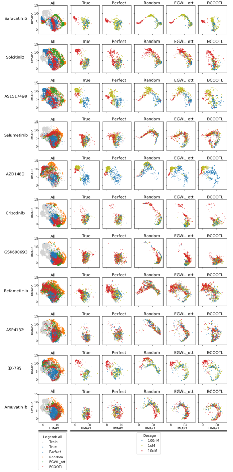
Figure 3: UMAPs of predicted cells

Match matrices

We show the mean couplings of ECOOTL and EGWL for 5 cross-validation folds in Figure 4. Whereas the negative controls (Vehicle, No stim) showed no clear separation of samples by the treatment dosages, we see the clustering of cells with the same dosages of the drugs.

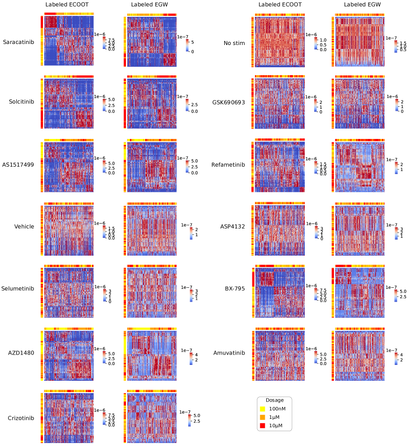
Figure 4: Mean couplings of ECOOTL and EGWL for 5 cross-validation folds. Rows are hierarchically clustered and columns are reordered by the same row order. Rows and columns are labeled by the dosage.

References

- Alvarez-Melis & Fusi (2020) Alvarez-Melis, D. and Fusi, N. Geometric dataset distances via optimal transport. In Advances in Neural Information Processing Systems, volume 33, pp. 21428–21439, 2020.
- Alvarez-Melis & Jaakkola (2018) Alvarez-Melis, D. and Jaakkola, T. Gromov-Wasserstein alignment of word embedding spaces. In Empirical Methods in Natural Language Processing, pp. 1881–1890, 2018.
- Alvarez-Melis et al. (2018) Alvarez-Melis, D., Jaakkola, T., and Jegelka, S. Structured optimal transport. In Artificial Intelligence and Statistics, volume 84, pp. 1771–1780, 2018.
- Ashuach et al. (2023) Ashuach, T., Gabitto, M. I., Koodli, R. V., Saldi, G.-A., Jordan, M. I., and Yosef, N. MultiVI: deep generative model for the integration of multimodal data. Nature Methods, 20(8):1222–1231, 2023.
- Bock et al. (2022) Bock, C., Datlinger, P., Chardon, F., Coelho, M. A., Dong, M. B., Lawson, K. A., Lu, T., Maroc, L., Norman, T. M., Song, B., Stanley, G., Chen, S., Garnett, M., Li, W., Moffat, J., Qi, L. S., Shapiro, R. S., Shendure, J., Weissman, J. S., and Zhuang, X. High-content CRISPR screening. Nature Reviews Methods Primers, 2(1):8, 2022.
- Bunne et al. (2023) Bunne, C., Stark, S. G., Gut, G., Del Castillo, J. S., Levesque, M., Lehmann, K.-V., Pelkmans, L., Krause, A., and Rätsch, G. Learning single-cell perturbation responses using neural optimal transport. Nature Methods, 20(11):1759–1768, 2023.
- Chuang et al. (2023) Chuang, C.-Y., Jegelka, S., and Alvarez-Melis, D. InfoOT: Information maximizing optimal transport. In International Conference on Machine Learning, volume 202, pp. 6228–6242, 2023.
- Chung et al. (2021) Chung, H., Parkhurst, C. N., Magee, E. M., Phillips, D., Habibi, E., Chen, F., Yeung, B. Z., Waldman, J., Artis, D., and Regev, A. Joint single-cell measurements of nuclear proteins and RNA in vivo. Nature Methods, 18(10):1204–1212, 2021.
- Comiter et al. (2023) Comiter, C., Vaishnav, E. D., Ciampricotti, M., Li, B., Yang, Y., Rodig, S. J., Turner, M., Pfaff, K. L., Jané-Valbuena, J., Slyper, M., Waldman, J., Vigneau, S., Wu, J., Blosser, T. R., Segerstolpe, Å., Abravanel, D., Wagle, N., Zhuang, X., Rudin, C. M., Klughammer, J., Rozenblatt-Rosen, O., Kobayash-Kirschvink, K. J., Shu, J., and Regev, A. Inference of single cell profiles from histology stains with the Single-Cell omics from histology analysis framework (SCHAF). bioRxiv, 2023.
- Courty et al. (2017) Courty, N., Flamary, R., Habrard, A., and Rakotomamonjy, A. Joint distribution optimal transportation for domain adaptation. In Advances in Neural Information Processing Systems, pp. 3733–3742, 2017.
- Cuturi (2013) Cuturi, M. Sinkhorn distances: Lightspeed computation of optimal transport. In Advances in Neural Information Processing Systems, volume 26, 2013.
- Cuturi et al. (2022) Cuturi, M., Meng-Papaxanthos, L., Tian, Y., Bunne, C., Davis, G., and Teboul, O. Optimal transport tools (OTT): A JAX toolbox for all things Wasserstein, 2022.
- Damodaran et al. (2018) Damodaran, B., Kellenberger, B., Flamary, R., Tuia, D., and Courty, N. DeepJDOT: Deep joint distribution optimal transport for unsupervised domain adaptation. European Conference on Computer Vision, 2018.
- Demetci et al. (2022a) Demetci, P., Santorella, R., Sandstede, B., Noble, W. S., and Singh, R. SCOT: Single-cell multi-omics alignment with optimal transport. Journal of Computational Biology, 29(1):3–18, 2022a.
- Demetci et al. (2022b) Demetci, P., Tran, Q. H., Redko, I., and Singh, R. Jointly aligning cells and genomic features of single-cell multi-omics data with co-optimal transport. bioRxiv, pp. 2022.11.09.515883, 2022b.
- Dixit et al. (2016) Dixit, A., Parnas, O., Li, B., Chen, J., Fulco, C. P., Jerby-Arnon, L., Marjanovic, N. D., Dionne, D., Burks, T., Raychowdhury, R., Adamson, B., Norman, T. M., Lander, E. S., Weissman, J. S., Friedman, N., and Regev, A. Perturb-Seq: Dissecting molecular circuits with scalable single-cell RNA profiling of pooled genetic screens. Cell, 167(7):1853–1866.e17, 2016.
- Feldman et al. (2019) Feldman, D., Singh, A., Schmid-Burgk, J. L., Carlson, R. J., Mezger, A., Garrity, A. J., Zhang, F., and Blainey, P. C. Optical pooled screens in human cells. Cell, 179(3):787–799.e17, 2019.
- Frangieh et al. (2021) Frangieh, C. J., Melms, J. C., Thakore, P. I., Geiger-Schuller, K. R., Ho, P., Luoma, A. M., Cleary, B., Jerby-Arnon, L., Malu, S., Cuoco, M. S., et al. Multimodal pooled perturb-cite-seq screens in patient models define mechanisms of cancer immune evasion. Nature Genetics, 53(3):332–341, 2021.
- Ganin et al. (2016) Ganin, Y., Ustinova, E., Ajakan, H., Germain, P., Larochelle, H., Laviolette, F., March, M., and Lempitsky, V. Domain-adversarial training of neural networks. Journal of Machine Learning Research, 17(59):1–35, 2016.
- Gayoso et al. (2022) Gayoso, A., Lopez, R., Xing, G., Boyeau, P., Valiollah Pour Amiri, V., Hong, J., Wu, K., Jayasuriya, M., Mehlman, E., Langevin, M., et al. A python library for probabilistic analysis of single-cell omics data. Nature Biotechnology, 40(2):163–166, 2022.
- Geiger-Schuller et al. (2023) Geiger-Schuller, K., Eraslan, B., Kuksenko, O., Dey, K. K., Jagadeesh, K. A., Thakore, P. I., Karayel, O., Yung, A. R., Rajagopalan, A., Meireles, A. M., Yang, K. D., Amir-Zilberstein, L., Delorey, T., Phillips, D., Raychowdhury, R., Moussion, C., Price, A. L., Hacohen, N., Doench, J. G., Uhler, C., Rozenblatt-Rosen, O., and Regev, A. Systematically characterizing the roles of e3-ligase family members in inflammatory responses with massively parallel perturb-seq. bioRxiv, 2023. doi: 10.1101/2023.01.23.525198.
- Gossi et al. (2023) Gossi, F., Pati, P., Chouvardas, P., Martinelli, A. L., Kruithof-de Julio, M., and Rapsomaniki, M. A. Matching single cells across modalities with contrastive learning and optimal transport. Briefing in Bioinformatics, 24(3), 2023.
- Kantorovich (1960) Kantorovich, L. Mathematical methods of organizing and planning production. Management science, 6(4):366– 422, 1960.
- Kodali et al. (2017) Kodali, N., Abernethy, J., Hays, J., and Kira, Z. On convergence and stability of GANs. arXiv, 2017.
- Liu et al. (2019) Liu, J., Huang, Y., Singh, R., Vert, J.-P., and Noble, W. S. Jointly embedding multiple Single-Cell omics measurements. In Algorithms in Bioinformatics, volume 143, 2019.
- Lopez et al. (2019) Lopez, R., Nazaret, A., Langevin, M., Samaran, J., Regier, J., Jordan, M. I., and Yosef, N. A joint model of unpaired data from scRNA-seq and spatial transcriptomics for imputing missing gene expression measurements. ICML Workshop in Computational Biology, 2019.
- Mémoli (2011) Mémoli, F. Gromov–Wasserstein distances and the metric approach to object matching. Foundations of Computational Mathematics, 11(4):417–487, 2011.
- Monge (1781) Monge, G. Mémoire sur la théorie des déblais et des remblais. Mémoires de l’Académie royale des sciences de Paris, 1781.
- Peyré & Cuturi (2018) Peyré, G. and Cuturi, M. Computational Optimal Transport. Foundations and Trends in Machine Learning, 2018.
- Peyré et al. (2016) Peyré, G., Cuturi, M., and Solomon, J. Gromov-Wasserstein averaging of kernel and distance matrices. International Conference on Machine Learning, pp. 2664–2672, 2016.
- Redko et al. (2020) Redko, I., Vayer, T., Flamary, R., and Courty, N. Co-optimal transport. Advances in Neural Information Processing Systems, 33(17559-17570):2, 2020.
- Wolf et al. (2018) Wolf, F. A., Angerer, P., and Theis, F. J. SCANPY: large-scale single-cell gene expression data analysis. Genome Biol., 19(1):15, 2018.
- Yeaton et al. (2022) Yeaton, A., Krishnan, R. G., Mieloszyk, R., Alvarez-Melis, D., and Huynh, G. Hierarchical optimal transport for comparing histopathology datasets. In Medical Imaging with Deep Learning, volume 172, pp. 1459–1469, 2022.