Astrophysical constraints from synchrotron emission
on very massive decaying dark matter

Abstract

If the cosmological dark matter (DM) couples to Standard Model (SM) fields, it can decay promptly to SM states in a highly energetic hard process, which subsequently showers and hadronizes to give stable particles including $e^{\pm}$, $\gamma$, $p^{\pm}$ and $\nu\bar{\nu}$ at lower energy. If the DM particle is very heavy, the high-energy $e^{\pm}$, due to the Klein-Nishina cross section suppression, preferentially lose energy via synchrotron emission which, in turn, can be of unusually high energies. Here, we present novel bounds on heavy decaying DM up to the Planck scale, by studying the synchrotron emission from the $e^{\pm}$ produced in the ambient Galactic magnetic field. In particular, we explore the sensitivity of the resulting constraints on the DM decay width to (i) different SM decay channels, to (ii) the Galactic magnetic field configurations, and (iii) to various different DM density profiles proposed in the literature. We find that constraints from the synchrotron component complement and improve on constraints from very high-energy cosmic-ray and gamma-ray observatories targeting the prompt emission when the DM is sufficiently massive, most significantly for masses in excess of $10^{12}\text{ GeV}$.

I Introduction

Observations of the dynamics of galaxy clusters, galactic rotation curves, the Cosmic Microwave Background (CMB) and large scale structure provide strong evidence for the existence of Dark Matter (DM). In particular, DM must be stable on cosmological time scales Poulin et al. (2016); Audren et al. (2014). If the DM is a particle that interacts with the Standard Model (SM), its possible decay to SM states allows us to place even stronger bounds on its lifetime. If the DM mass $m_{\chi}$ is large, the decay process $\chi\to\text{SM+SM}$ produces the SM states with an energy $\mu\sim m_{\chi}/2$; such states subsequently hadronize and shower to produce photons, electrons/positrons, protons/anti-protons and neutrinos below the electroweak (EW) scale Bauer et al. (2021).

The effort in searching for photons from DM annihilation and/or decay, part of the broader multi-messenger “indirect DM detection” campaign, is at a very advanced stage (for a pedagogical review, see Slatyer (2022)). In particular, the leading facilities probing the DM particle lifetime indirectly through its final decay products, such as photons, neutrinos and cosmic rays, include the Fermi Large Area Telescope (Fermi-LAT) Huang et al. (2012); Song et al. (2023); Ackermann et al. (2012), the Pierre Auger Observatory (PAO) Aloisio (2023), the High-Altitude Water Cherenkov Observatory (HAWC) Abeysekara et al. (2018); Albert et al. (2023), the Large High Altitude Air Shower Observatory (LHAASO) Cao et al. (2022) and IceCube Aartsen et al. (2018); Abbasi et al. (2023); Esmaili and Serpico (2013); Chianese et al. (2019). In addition, upcoming experiments including the Cherenkov Telescope Array (CTA) Acharya et al. (2018); Pierre et al. (2014); Acharyya et al. (2021) and IceCube-Gen2 Aartsen et al. (2021); Fiorillo et al. (2023) are expected to ramp up the reach of future indirect DM detection campaigns.

The products of the prompt decay of DM into SM particles are not exhaustive of the entirety of the emission eventually arising from the decay event. Stable, charged particles, electrons and positrons ($e^{\pm}$) and protons and antiprotons, lose energy to a variety of electromagnetic processes that, in turn, produces lower-energy radiation. Due to the difference in particle mass, the emission from $e^{\pm}$ is both brighter and higher-energy than that from hadrons, albeit it does not include inelastic processes. As a function of the $e^{\pm}$ energy, from low to high energy, the principal energy loss mechanisms are, typically, Coulomb losses, bremsstrahlung, Inverse Compton (IC), and synchrotron Longair (1992). The first detailed calculation of the broad band emission from a specific class of weakly-interacting massive particles (WIMPs), supersymmetric neutralinos, was carried out in Ref. Colafrancesco et al. (2006, 2007) (see also Profumo and Ullio (2010) for a review). Since then, several other studies have investigated the prompt emission, Inverse Compton emission and synchrotron emission for WIMP-like, electroweak-scale DM masses (an incomplete list includes Ref. Hutsi et al. (2010); Cohen et al. (2017); Blanco and Hooper (2019)), while other studies have explored the prompt and IC emission for superheavy DM Esmaili and Serpico (2015); Kalashev et al. (2021); Chianese et al. (2021a); Esmaili and Serpico (2021); Chianese et al. (2021b); Skrzypek et al. (2021). Ref. Deliyergiyev et al. (2022) derives constraints on superheavy DM combining prompt emission with gravitational wave observations.

In this paper, to our knowledge for the first time, we focus on bounds obtained from synchrotron emission emanating from superheavy DM decays. The best observational target to search for this signal is by far the Galactic center. Here, we intend to assess whether the synchrotron emission, at much lower energy than the prompt and IC emission, provides comparable or more competitive bounds on the DM lifetime. The peak frequency of the synchrotron emission depends linearly on the ambient magnetic field, and quadratically on the electron energy. In particular, we will show that the peak energy of the synchrotron emission, in the Galactic center region, scales with the DM mass $m_{\chi}$, approximately as

$$\frac{E_{\rm peak}}{\rm GeV}\simeq\left(\frac{m_{\chi}}{10^{10}\ {\rm GeV}}\right)^{2}.$$ (1)

As a result, the synchrotron emission falls squarely in the high-energy gamma-ray range where Fermi-LAT is sensitive (roughly between 0.1 GeV and 1 TeV) for $10^{9}\lesssim m_{\chi}/{\rm GeV}\lesssim 10^{12}$; in the very high-energy Cherenkov telescope range (roughly 0.1 TeV to 1,000 TeV) for $10^{11}\lesssim m_{\chi}/{\rm GeV}\lesssim 10^{14}$; and, at even larger masses, at ultra high-energy cosmic-ray/gamma-ray facilities.

The principal goal of the present study is to understand in detail how the predicted synchrotron emission depends on the assumed Galactic magnetic model, on the DM density distribution in the Galaxy, on the $e^{\pm}$ injection spectrum, and the signal morphology. To this end, we first review, in Section II, the calculation of the prompt gamma-ray emission , the $e^{\pm}$ injection spectrum, the subsequent energy losses, and the resulting synchrotron emission. In Section III, we elaborate on the dependence of the signal on the Galactic magnetic field model and on the DM density profiles that we implement. In Section IV, we briefly describe the experimental limits set by astrophysical multimessenger experiments (Fermi-LAT, HESS, Pierre-Auger Observatory, CASA-MIA, KASCADE, KASCADE-GRANDE, PAO, TASD and EAS-MSU) on the observed photon flux from the Galactic center. In Section V, we compute the synchrotron fluxes for various initial SM states and we present novel constraints on the lifetime of the DM depending on its mass. Finally, we summarize our findings and present our outlook in Section VI.

II Multi-wavelength Emission From Dark Matter Decay

Here we review schematically the production of photons from heavy DM decay, both via prompt production (sec. II.1) and via synchrotron emission off of the prompt $e^{\pm}$ (sec. II.2).

II.1 Prompt Emission

The differential flux of photons from DM decay from a given line of sight is given by Esmaili and Serpico (2015)

$$\frac{d\Phi}{dE_{\gamma}}=\frac{1}{4\pi m_{\chi}\tau_{\chi}}\frac{dN}{dE_{\gamma}}\int_{0}^{\infty}ds\,\rho(s,b,l)e^{-\tau_{\gamma\gamma}(E_{\gamma},s,b,l)}$$ (2)

where $E_{\gamma}$ is the photon energy, $m_{\chi}$ is the DM mass, $\tau_{\chi}$ is the DM lifetime, $\rho$ is the Galactic DM density profile, $s$ is the line-of-sight distance from the observer, and $b,l$ are the Galactic latitude and longitude angular coordinates respectively. $dN/dE_{\gamma}$ is the energy spectrum of photons produced per decay and $\tau_{\gamma\gamma}$ is the optical depth due to pair production against Cosmic Microwave Background (CMB), starlight (SL) and infrared (IR) photons.

The energy spectrum $dN/dE_{\gamma}$ is obtained from HDMSpectra Bauer et al. (2021) which incorporates EW corrections that become important at higher energies.

The optical depth $\tau_{\gamma\gamma}$, which characterizes the impact of the absorption of gamma rays in the interstellar medium, has a noticeable effect on the spectrum mostly in the range of energies $E_{\gamma}\simeq 10^{4}-10^{8}$ GeV. Our analysis neglects the optical depth entirely since we expect that the constraints we derive from high energy gamma-ray probes of the integrated flux (see the discussion in Section IV) suffer from at most $O(1)$ corrections due to the effects of attenuation from the Galactic center to the Earth. Please see Refs. Esmaili and Serpico (2021); De Angelis et al. (2013) for more details about the flux attenuation. Of course this assumption is invalid for extragalactic DM decays.

II.2 Synchrotron emission

Relativistic electrons in the Galactic magnetic field produce synchrotron radiation BLUMENTHAL and GOULD (1970). At very high energy, typical of the $e^{\pm}$ produced by the decay of very massive DM, the inverse Compton Klein-Nishina cross section is highly suppressed compared to the corresponding synchrotron emission process. The differential synchrotron component of the gamma ray flux (after setting the optical depth to zero) is given by

$$\frac{d\Phi}{dE_{\gamma}d\Omega}(E_{\gamma},b,l)=\frac{1}{4\pi E_{\gamma}}\int_{m_{e}}^{m_{\chi}/2}dE_{e}\,\int_{0}^{\infty}ds\,\frac{dn_{e}}{dE_{e}}(E_{e},s,b,l)P_{\rm syn}(E_{\gamma},E_{e},s,b,l),$$ (3)

where $m_{e}$ is the mass of the electron and $d\Omega=\cos b\,db\,dl$ is the solid angle. The formula for the synchrotron power $P_{\rm syn}$ is provided in Appendix A. The steady-state equilibrium electron number density after energy losses and diffusion, is given by

$$\frac{dn_{e}}{dE_{e}}(E_{e},s,b,l)=\frac{1}{m_{\chi}\tau_{\chi}}\frac{\rho(s,b,l)}{b_{\rm tot}(E_{e},s,b,l)}\int^{m_{\chi}/2}_{E_{e}}\frac{dN}{dE_{e}^{\prime}}I(E_{e},E_{e}^{\prime},s,b,l)\,dE_{e}^{\prime},$$ (4)

where $b_{\rm tot}=-dE_{e}/dt$ is the total energy loss coefficient comprising energy losses due to Inverse Compton (IC) scattering of electrons on CMB, SL and IR photons ($b_{\rm IC}$), triplet pair production (TPP) energy losses ($b_{\rm TPP}$) Mastichiadis (1991) and synchrotron energy losses ($b_{\rm syn}$). As mentioned above, for superheavy DM (which subsequently produce ultrarelativistic electrons below the EW scale), we verified that TPP and IC energy losses are negligible when compared to synchrotron i.e. $b_{\rm TPP},b_{\rm IC}\ll b_{\rm syn}$ so that taking

$$b_{\rm tot}\simeq b_{\rm syn}$$ (5)

is entirely sufficient for our purposes. Details about the computation of the energy losses are found in Appendix B.

Similarly to the prompt photon emission, the injected energy spectrum of electrons $dN/dE_{e}$ is obtained from HDMSpectra, whereas the diffusion halo function $I$ can be solved from the diffusion-loss equation as discussed in Ref. Cirelli et al. (2011) (see also Colafrancesco et al. (2006)). At high injection energies, $I\simeq 1$ Cirelli et al. (2011); Esmaili and Serpico (2015). Defining $x=2E_{e}/m_{\chi}$, we thus have:

$$\frac{dn_{e}}{dE_{e}}\simeq\frac{1}{m_{\chi}\tau_{\chi}}\frac{\rho(s,b,l)}{b_{\rm tot}(E_{e},s,b,l)}\int^{1}_{2\frac{E_{e}}{m_{\chi}}}\frac{dN}{dx}\,dx.$$ (6)

Replacing the electron number density from equation (6) and $P_{\rm syn}$ from equation (16) into equation (3), we are able to find the differential flux in a given angular region along a certain direction ($b,l$) in the sky.

For reference, we also list the angular averaged flux over the unit sphere $S^{2}$ given by

$$\frac{d\Phi}{dE_{\gamma}}(E_{\gamma})\Bigg{|}_{S^{2}\text{ avg}}=\frac{1}{4\pi}\int_{S^{2}}d\Omega\frac{d\Phi}{dE_{\gamma}d\Omega}$$ (7)

and the angular averaged $E_{\gamma}$ integrated flux,

$$\Phi(E_{\gamma})=\frac{1}{4\pi}\int_{S^{2}}d\Omega\int_{E_{\gamma}^{\prime}}^{\frac{m_{\chi}}{2}}dE_{\gamma}^{\prime}\frac{d\Phi}{d\Omega dE_{\gamma}^{\prime}}$$ (8)

Both of these quantities will be useful during the discussion in Section IV.

III Astrophysical inputs: Magnetic field and DM density

In this Section, we summarize the Galactic magnetic field models (in III.1) and DM density profiles (in III.2) implemented in our study.

III.1 Magnetic field models

The morphology of the Galactic magnetic field (GMF) is highly uncertain due to the lack of direct measurements Jansson and Farrar (2012a); Unger and Farrar (2018). A number of GMF models have been proposed in the literature with different functional forms Sun et al. (2008); Sun and Reich (2010); Jaffe et al. (2013). For recent reviews on the GMF and modeling efforts, see also Refs. Jaffe (2019); Ferrière, Katia (2023).

Here, we employ the Jansson and Farrar (JF12) magnetic field model as our benchmark Jansson and Farrar (2012a, b). This model uses the WMAP7 Galactic Synchrotron Emission map and more than forty thousand extragalactic rotation measures to fit the model parameters to observations. JF12 consists of a disk field and an extended halo field, both containing large scale regular field, small scale random field and striated random field components. Detailed information about the implementation of the JF12 model and its parameters can be found in Refs. Jansson and Farrar (2012a, b). During the preparation of this work, we became aware of Ref. Unger and Farrar (2023) which analyses variants of the coherent disk, poloidal and toroidal halo fields, free from discontinuities, together with variants for the thermal and cosmic-ray electron densities, to finally converge to an optimized set of eight fitted GMF models. The parametric models employed in the fitting procedure are more complex but many similarities regarding the overall structure of the GMF models are shared with JF12. Most importantly, the magnetic field strength of the fitted ensemble are of the same order as JF12. Therefore, we expect that our results are largely insensitive and qualitatively unaffected by the updated model in Ref. Unger and Farrar (2023).

Instead of realizing a stochastic implementation of the random and random striated components, we adopt the estimate discussed in Jansson and Farrar (2012a, b), i.e. we approximate the rms value of the striated component by $B^{2}_{\rm stri}=\beta B^{2}_{\rm reg}$, whereas the relativistic electron density is rescaled by a factor $n_{e}\to\alpha n_{e}$, where $\alpha$ and $\beta$ are parameters of the fitted JF12 model. Hence in our formula for $b_{\rm syn}$, we calculate $B$ using the prescription

$$B=\sqrt{(\beta+1)B_{\rm reg}^{2}+B_{\rm ran}^{2}}$$ (9)

where $B_{\rm ran}$ is the rms value of the random component. Since the synchrotron flux is proportional to $n_{e}$ and the perpendicular component (squared) $B_{\perp}^{2}=B^{2}\sin^{2}\theta$, we make the replacement

$$B_{\perp}^{2}\to\alpha(1+\beta)B^{2}_{\rm reg}\sin^{2}\theta+\frac{2}{3}\alpha B^{2}_{\rm ran}$$ (10)

in $P_{\rm syn}$ where the factor of $(2/3)$ comes from averaging isotropically. Equations (9) and (10) suffice to provide an accurate estimate of the synchrotron emission using the JF12 model, as we verified by comparing the assumed synchrotron energy losses with the synchrotron emission integrated over energy.

Ref. Adam et al. (2016) gives updated parameters for the JF12 model by including information about the total and polarized dust emission, as well as synchrotron at low frequency (30 GHz) from Planck data. In particular, the Jansson 12b (JF12b) model is adjusted to match the synchrotron emission while the Jansson 12c (JF12c) model is adjusted to match the dust emission while trying to retain the features of JF12b. We further emphasize that neither JF12b nor JF12c give best-fit results to the data but only indicate how the original JF12 model parameters could be improved.

Finally, due to its simplicity, we also implement the MF1 model as defined in Ref. Cirelli et al. (2011) (see also Refs. Perelstein and Shakya (2011); Strong and Moskalenko (1999)). MF1 only consists of a regular component for the disk field

$$B(s,b,l)=B_{0}\exp\left[{-\frac{|r_{\rm cyl}-R_{\odot}|}{r_{B}}-\frac{|z|}{z_{B}}}\right]$$ (11)

where $r_{\rm cyl}=\sqrt{s^{2}\cos^{2}(b)+R_{\odot}^{2}-2sR_{\odot}\cos(b)\cos(l)}$ is the galactocentric radius, $z=s\sin(b)$, $R_{\odot}=8.3\text{ kpc}$, $r_{B}=10\text{ kpc}$, $z_{B}=2\text{ kpc}$ and $B_{0}=4.78~{}\mu G$. We caution that MF1 is an over-simplified model of the GMF as it does not contain a halo field and additionally fails to capture any turbulent components of the GMF. Since we aim to compare our results from JF12 with arguably the simplest GMF model, we refrain from augmenting MF1 with halo field or turbulent field components.

III.2 DM density profiles

The determination of the distribution of DM at the Galactic center suffers from a large degree of uncertainty due to the axisymmetric Galactic bar and non-circular streaming motions Sofue (2013). Therefore, we find it prudent to explore the sensitivity of our results to different DM density profiles which are summarized below.

We choose as our benchmark the standard Navarro–Frenk–White (NFW) profile for the DM density Navarro et al. (1996, 1997).

$$\rho_{\rm NFW}(r)=\frac{\rho_{h}}{\frac{r}{r_{s}}\left(1+\frac{r}{r_{s}}\right)^{2}}$$ (12)

where $r$ is the spherical coordinate

$$r=\sqrt{s^{2}+R{{}_{\odot}}^{2}-2sR_{\odot}\cos(b)\cos(l)}$$ (13)

and $\rho_{h}=0.18\text{ GeVcm}^{-3}$, $r_{s}=24\text{ kpc}$ is the scale radius.

In addition to the NFW profile, we also consider its generalized form (gNFW), given by

$$\rho_{\rm gNFW}(r)=\frac{M_{0}}{4\pi r_{s}^{3}}\frac{1}{\left(\frac{r}{r_{s}}\right)^{\beta}\left(1+\frac{r}{r_{s}}\right)^{3-\beta}}$$ (14)

Ref. Lim et al. (2023) gives the best-fit values $M_{0}=1.3778\times 10^{11}M_{\odot}$, $r_{s}=3.6$ kpc and $\beta=1.1$, whereas Ref. Ou et al. (2023) gives $M_{0}=3.21\times 10^{11}M_{\odot}$, $r_{s}=5.26\text{ kpc}$ and $\beta=0.0258$. We will refer to the first set of parameter values as gNFWLim and the second set as gNFWOu.

Finally, we also consider the Einasto (EIN) profile

$$\rho_{\rm Ein}(r)=\frac{M_{0}}{4\pi r_{s}^{3}}e^{-(r/r_{s})^{\alpha}};$$ (15)

for the EIN input parameters, Ref. Ou et al. (2023) finds $M_{0}=0.62\times 10^{11}M_{\odot}$, $r_{s}=3.86\text{ kpc}$ and $\alpha=0.91$. We note that Ref. Ou et al. (2023) argues that the Einasto profile is statistically preferred compared to the gNFWOu profile as a best-fit to the Milky Way Galactic rotation curve.

IV Observational limits

We investigate the experimental limits on the photon flux from the Galactic center in a range of photon energies.

At low energies i.e. $E_{\gamma}\sim 10^{-1}-50$ GeV, limits on the photon flux are set by the space-based gamma-ray telescope Fermi-LAT. In our analysis, we use the limits provided by Ref. Picker and Kusenko (2023) where the flux is integrated over an angular region of $\Delta\Omega=2\pi(1-\cos\theta)$ with $\theta=1^{\circ}$ being the angle between the line of sight direction and direction of the Galactic center.

In the energy range $E_{\gamma}\sim 200-5\times 10^{4}$ GeV, measurements from the ground-based Cherenkov telescope HESS are the most competitive, constraining the observed (differential) photon flux integrated over an annular region with $\theta=0.5^{\circ}-3.0^{\circ}$ Abdalla et al. (2022). The energy-dependent acceptance of the instrument is obtained from Ref. de Naurois and Rolland (2009).

For heavy $m_{\chi}\gtrsim 10^{12}$ GeV, most of the flux occurs at higher energies $E_{\gamma}\gtrsim 10^{4}$ GeV (as can be seen in the bottom left panel of Fig. 2). In this region, we obtain limits on the angular averaged flux (defined in eq. (7)) from the Pierre-Auger Observatory (PAO) Ishiwata et al. (2020). To speed up the computation of the angular average, we uniformly sample ten points on the unit sphere according to the algorithm laid out in Deserno (2004) and find the averaged flux over the sampled points. The sample size was optimal as it provided a reliable approximation to samples that included more points, at the price of significantly greater computational cost.

Moreover, CASA-MIA, KASCADE, KASCADE-GRANDE, PAO, TASD and EAS-MSU all provide limits on the (energy) integrated (angular averaged) flux in eq. (8) Chianese et al. (2021a). Henceforth we will collectively refer to these limits as ‘Chianese et al.’.

To obtain constraints on the DM lifetime, we require that the photon flux (either synchrotron or prompt) does not exceed the flux measured by the above experiments over the respective energy ranges. We thus very conservatively neglect any photon source besides DM decay (in reality part or most of the emission has other astrophysical origins).

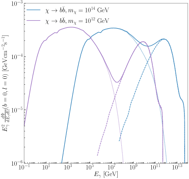
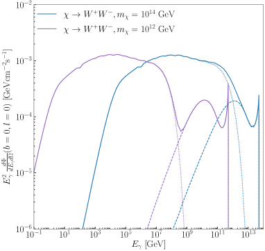
Figure 1: Plot of differential photon flux spectra for $b\bar{b}$ (Left) and for $W^{+}W^{-}$ (Right) final states. In blue is the flux for DM of mass $m_{\chi}=10^{14}$ GeV and in purple is the flux for DM of mass $m_{\chi}=10^{12}$ GeV. The prompt and synchrotron contributions to the flux are shown as dotted and dashed lines respectively, while the combined flux is represented by solid lines.

V Results

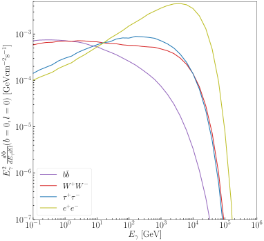
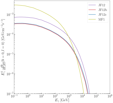
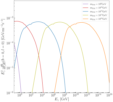
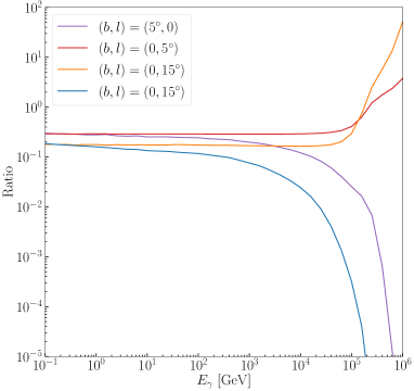
Figure 2: The SM initial state, GMF, dark matter mass, and the angular location are taken to be $b\bar{b}$, JF12, $m_{\chi}=10^{10}$ GeV and $(b,l)=(0,0)$ by default, with only one of them being varied in each plot. The variation of the differential photon synchrotron flux is depicted for different SM initial states $b\bar{b}$, $W^{+}W^{-}$, $\tau^{+}\tau^{-}$ and $e^{+}e^{-}$ (top left), different magnetic field models JF12, JF12b, JF12c and MF1 (top right), and the range of masses $m_{\chi}=10^{8}-10^{16}$ GeV (bottom left). Finally, the ratio of the differential photon synchrotron flux from different $(b,l)$ locations to the one from $(b,l)=(0,0)$ is shown (Bottom Right).

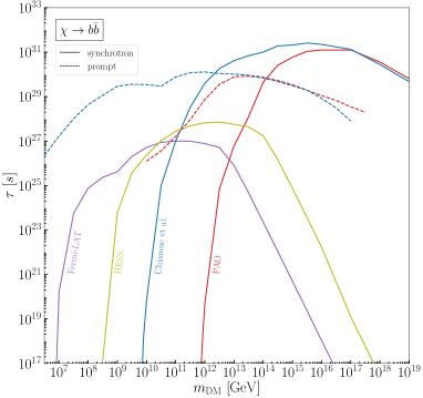
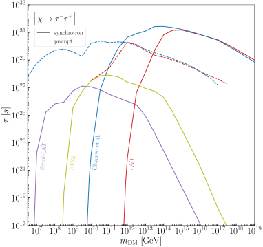
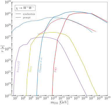
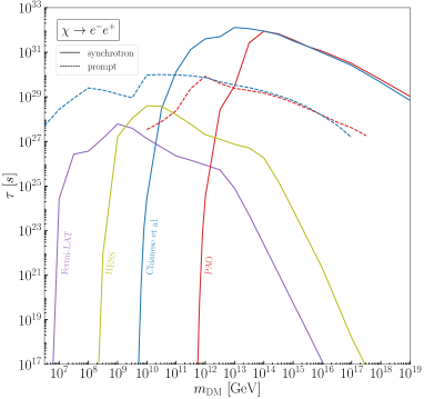
Figure 3: The constraints obtained from the different experiments on the lifetime of the DM $\tau_{\chi}$ as a function of the DM mass $m_{\chi}$ are shown. The constraints from Fermi-LAT ( purple), HESS (green) and PAO (red) are obtained from Refs. Picker and Kusenko (2023), Abdalla et al. (2022) and Ishiwata et al. (2020) respectively, whereas the constraint from the experiments considered in Ref. Chianese et al. (2019) are collectively denoted as ‘Chianese et al.’ ( blue). Each panel shows the constraints obtained for different initial SM states ($b\bar{b},\tau^{+}\tau^{-},W^{+}W^{-}$ and $e^{+}e^{-}$) for both the prompt (dashed lines) and the synchrotron (solid lines) components separately.

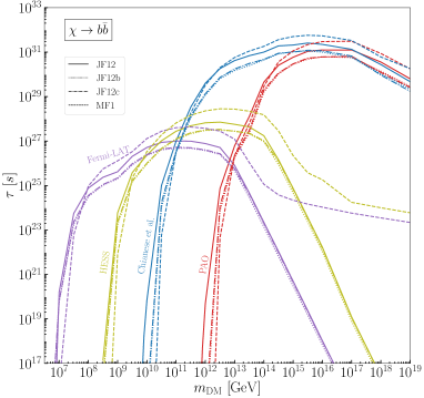
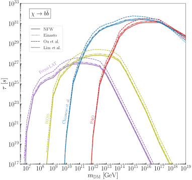
Figure 4: The constraints obtained from the different multimessenger experimental probes on the lifetime of the DM $\tau_{\chi}$ as a function of the DM mass $m_{\chi}$ are shown. (Left) The Galactic Magnetic Field profile is varied. (Right) The Dark Matter density profile is varied.

We start by showing, in Fig. 1, the prompt and synchrotron spectral energy density (SED) emission for decay final states into $b\bar{b}$ (left) and for $W^{+}W^{-}$ (right) final states. We show in blue results for a DM particle of mass $m_{\chi}=10^{14}$ GeV and in purple of mass $m_{\chi}=10^{12}$ GeV. The prompt and synchrotron contributions to the flux are shown as dotted and dashed lines respectively, while the combined flux is represented by solid lines. As expected, the flux for the two masses is relatively self similar, but at increasing masses the peak of the synchrotron emission moves to higher energies quadratically with $m_{\chi}$. Remarkably, the peak of the synchrotron SED emission surpasses the prompt emission to photons, indicating that the decay releases, eventually, more energy to $e^{\pm}$ than to prompt photons. Notice that in the $\bar{b}b$ case, $e^{\pm}$ stem from charged pion decay whereas photons arise from neutral pion decay, hence the height of the peak is comparable. In the $W^{\pm}$ case, we note the peak stemming from internal bremsstrahlung at the highest energies; the synchrotron emission is especially bright, including because of the $W\to e\nu_{e}$ decay mode.

In Fig. 2, the synchrotron differential flux $\frac{d\Phi}{dE_{\gamma}d\Omega}$ is shown as a function of $E_{\gamma}$. We choose as a benchmark the flux originating from the Galactic center (of Galactic coordinates $(b,l)=(0,0)$), with $m_{\chi}=10^{10}$ GeV, initial SM state $b\bar{b}$, JF12 magnetic field model and standard NFW DM profile. Each of the four panels shows the change in the flux with respect to one of these inputs being modified.

The top left panel shows the flux for different initial SM states namely $b\bar{b}$, $W^{+}W^{-}$, $\tau^{+}\tau^{-}$ and $e^{+}e^{-}$. We find that massive SM states such as the bottom quark and $W$ tend to have a flatter spectrum than lighter states such as the $\tau$ and the electron which have a more peaked spectrum. This can be ascribed to the production mechanisms associated with each final state: bottom quarks produce photons primarily by the decay of byproducts of the hadronization process, eventually leading to neutral pions decaying preferentially to two photons; $e^{\pm}$ produce copious internal bremsstrahlung photons, whereas $W^{\pm}$ and $\tau^{\pm}$ both produce photons from internal bremsstrahlung and from hadronic channels.

The top right panel shows the variation of the flux with the different magnetic field configurations: MF1, JF12, JF12b and JF12c, all discussed and detailed upon in Section III.1 above. Notice that JF12b and JF12c are extremely close, and JF12 enhances the synchrotron emission by a factor of around 2, indicating that the magnetic field is within 50% of the JF12b and JF12c models; the only qualitative outlier is the MF1 model, which misses a number of features such as halo field and turbulent field components included in the other models. Most conspicuously the synchrotron emission computed with the MF1 model has a much softer spectrum that over-shoots that from the JF models by almost one order of magnitude at low energy and under-shoots by similar amounts at high energy. It is relevant to mention that this behavior scales strongly with the DM mass: for example, for $m_{\chi}=10^{18}$ GeV, the synchrotron flux from MF1 dominates at low photon energies by up to ten orders of magnitude over that from JF12, implying much stronger constraints from Fermi-LAT and HESS in this region, as can be seen in Fig. 4. Nevertheless, we reiterate that due to the crudeness of MF1, the constraints there are not expected to be physical, as they deviate too far from the more reliable and complete JF12 models.

The bottom left panel shows the flux for a range of DM masses from $m_{\chi}=10^{8}$ to $10^{16}$ GeV. As the DM mass increases, the peak of the spectrum also appears at higher photon energies, as expected. As indicated in the Introduction, we find that the peak emission occurs at $E_{\rm peak}/{\rm GeV}\simeq(m_{\chi}/(10^{10}\ {\rm GeV}))^{2}$.

Finally, the bottom right panel shows the angular variation of the flux at different Galactic angular coordinates $(b,l)=(5^{\circ},0)$, $(b,l)=(0,5^{\circ})$, $(b,l)=(15^{\circ},0)$ and $(b,l)=(0,15^{\circ})$ as compared to the flux from the Galactic center (GC). As expected, the GC direction dominates at all energy, mostly because of a higher DM density along the line of sight. However, interestingly enough, at higher Galactic longitudes, along the Galactic plane ($b=0$), we find a larger emission at high energy than in the GC direction: this is presumably due to a complex combination of effects related to the injected electron equilibrium spectrum and the magnetic field along the line of sight compensating and out-doing the smaller DM density.

In Fig. 3, we derive constraints on the DM lifetime $\tau_{\chi}$ as a function of its mass $m_{\chi}$, and compare with the corresponding constraints from prompt emission. Each panel shows the bounds obtained for the different initial SM states $b\bar{b},W^{+}W^{-},\tau^{+}\tau^{-},e^{+}e^{-}$. The red, blue, purple, green lines show the constraints derived from the Pierre-Auger observatory Ishiwata et al. (2020), ‘Chianese et al.’ Chianese et al. (2021a), Fermi-LAT Picker and Kusenko (2023) and HESS Abdalla et al. (2022) respectively, with the solid lines corresponding to the synchrotron emission and the dashed lines from the prompt emission (which, in the range of masses under consideration corresponds to the Chianese et al and PAO limits). We note that for all final states, the synchrotron component provides a significant improvement over the constraints coming from the prompt component only for $m_{\chi}\gtrsim 10^{12}\ {\rm GeV}$ by up to, and in some cases over one order of magnitude, while the prompt emission is more constraining, by a similar amount, up to one order of magnitude at lower masses $m_{\chi}\lesssim 10^{12}\ {\rm GeV}$.

In Fig. 4, we derive the same type of constraints from the synchrotron emission, but varying the astrophysical inputs for the magnetic field models (Left) and for different DM profiles (Right). In the left panel, the solid, dashed, dot-dashed and dotted lines represent the bounds from JF12, MF1, JF12c and JF12b respectively whereas in the right panel, they represent the bounds from NFW, gNFWLim, gNFWOu and Ein respectively. With the caveat discussed above about MF1, we find that our predictions are broadly subject to up to one order of magnitude uncertainty from the magnetic field model, and slightly less than that for the dark matter density. Note that the prompt emission is also subject to the latter range of uncertainty, but it is unaffected by the magnetic field. However, one should also note that HDMSpectra has considerable uncertainties when $x=2E_{e}/m_{\chi}$ is small, notably $x\lesssim 10^{-4}$. Hence we restrict $x\geq 10^{-4}$ for the synchrotron component and $x\geq 10^{-6}$ for the prompt component.

VI Conclusions and Outlook

We explored how gamma-ray telescopes such as Fermi-LAT and HESS, and high-energy observatories such as Pierre Auger and LHAASO, provide the most stringent constraints on the lifetime of heavy DM candidates, specifically heavier than $10^{12}$ GeV, by constraining the synchrotron emission generated by the very high-energy electrons and positrons produced in the decay, rather than the prompt gamma-ray emission. The synchrotron constraints are up to one order of magnitude stronger than constraints from the prompt emission by very high-energy cosmic-ray and gamma-ray facilities.

The synchrotron luminosity depends on the specific Galactic magnetic field model assumed; we showed, however, that for realistic, detailed magnetic field models the uncertainty is well below one order of magnitude, and comparable to the uncertainty associated with the dark matter density profile.

We showed that the synchrotron emission peaks at an energy $E_{\rm peak}/{\rm GeV}\simeq(m_{\chi}/(10^{10}\ {\rm GeV}))^{2}$, and is typically brighter in the direction of the Galactic center, i.e. for $(b,l)=(0,0)$, with the exception of very high energies, where it can be brighter at non-zero longitude along the Galactic plane, possibly offering a better signal-to-noise ratio as there the astrophysical backgrounds are typically lower.

In the future we plan to re-consider, with the present implementation of several up-to-date Galactic magnetic field models, limits from synchrotron emission of lighter DM candidates. We also plan to assess how information on polarization Manconi et al. (2022) could improve on the limits presented here, should future gamma-ray telescopes be sensitive to a polarized signal. Finally, the tools developed in this study will be made available by request to the Authors, and can be used to set constraints on concrete model-specific DM candidates.

Appendix A synchrotron power

The synchrotron power is calculated using Colafrancesco et al. (2006); Buch et al. (2015); Profumo and Ullio (2010)

$$P_{\rm syn}(E_{\gamma},E_{e},s,b,l)=\frac{\sqrt{3}}{2}\frac{e^{3}}{m_{e}}\int_{0}^{\pi}d\theta~{}B\sin^{2}\theta\,F\left(\frac{x}{\sin\theta}\right),$$ (16)

where $e$ is the electric charge and $B$ is the magnetic field. The other functions featuring in the integrand are

$$x =\frac{E_{\gamma}}{3\pi\nu_{0}\gamma^{2}}\left[1+\left(\gamma\frac{2\pi\nu_{p}}{E_{\gamma}}\right)^{2}\right]^{3/2}$$ (17)

$$F(t) =t\int_{t}^{\infty}dz\,K_{5/3}(z)$$ (18)

where $\gamma=\frac{E_{e}}{m_{e}}$ is the Lorentz boost factor, $\nu_{p}\simeq 8980\text{Hz}\left(\frac{n}{\text{cm}^{-3}}\right)^{1/2}$ is the plasma frequency, $\nu_{0}=(eB)/(2\pi m_{e})$ is the gyro-frequency, and $n\simeq 1\text{cm}^{-3}$ is the thermal electron number density.

Appendix B Energy losses

$e^{\pm}$ at high energies lose energy mainly through Inverse Compton (IC) scattering and triplet pair production processes (TPP) against CMB, SL and IR photons, as well as synchrotron radiation from being accelerated by the Galactic magnetic field.

$$b_{\rm tot}\simeq b_{\rm syn}+b_{\rm IC}+b_{\rm tpp}$$ (19)

The synchrotron energy loss is given by

$$b_{\rm syn}(E_{e})=\frac{4\sigma_{T}E_{e}^{2}}{3m_{e}^{2}}\frac{B^{2}}{2}$$ (20)

where $\sigma_{T}$ is the Thomson cross-section

$$\sigma_{T}=\frac{8\pi\alpha_{\rm em}^{2}}{3m_{e}^{2}}$$ (21)

with $\alpha_{\rm em}$ being the fine-structure constant.

The number density of photons (taking only the CMB component) at an energy $\epsilon$ is

$$n(\epsilon)=\frac{\epsilon^{2}}{\pi^{2}}\frac{1}{e^{\epsilon/T_{\rm CMB}}-1}$$ (22)

where we neglect the starlight and dust contributions. This is an excellent approximation since for highly energetic electrons (as typically produced from superheavy DM) with an energy above $E_{e}\gtrsim 50$ TeV, scattering with higher energy photons from SL and IR backgrounds are more Klein-Nishina suppressed Sudoh et al. (2021); Cirelli et al. (2011), and therefore contribute negligibly to the IC energy loss compared to the CMB.

The IC energy loss is obtained from the following expression

$$b_{\rm IC}(E_{e})=3\sigma_{T}\int_{0}^{\infty}d\epsilon\int_{1/(4\gamma^{2})}^{1}dq\,\epsilon\,n(\epsilon)\frac{(4\gamma^{2}-\Gamma)q-1}{(1+\Gamma q)^{3}}\left[2q\log q+q+1-2q^{2}+\frac{\Gamma^{2}q^{2}(1-q)}{2(1+\Gamma q)}\right]$$ (23)

where $\gamma=E_{e}/m_{e}$ is the Lorentz boost of the electron and $\Gamma(E_{e},\epsilon)=4\epsilon\gamma/m_{e}$.

Triplet pair production (TPP) $\gamma e\to 3e$ is an $O(\alpha_{\rm em}^{3})$ QED process where a photon interacts with an electron/positron to produce an electron-positron pair in addition to the original recoiling electron/positron. For highly energetic electrons, the energy loss by TPP becomes comparable to that of IC.

In the extreme Klein-Nishina limit ($\Gamma\gg 1$), Ref. Mastichiadis (1991) derives an analytical estimate of the energy loss valid in the regime $\gamma\epsilon\gtrsim 10^{3}\,m_{e}$,

$$b_{\rm tpp}(E_{e})\simeq\frac{15}{8}\sigma_{T}m_{e}^{2}\int d\epsilon\frac{n(\epsilon)}{\epsilon}\alpha_{\rm em}\left(\frac{\gamma\epsilon}{m_{e}}\right)^{1/4}\left[\frac{28}{9}\ln\left(\frac{2\gamma\epsilon}{m_{e}}\right)-\frac{218}{27}\right]~{}.$$ (24)

References

- Poulin et al. (2016) Vivian Poulin, Pasquale D. Serpico, and Julien Lesgourgues, “A fresh look at linear cosmological constraints on a decaying dark matter component,” JCAP 08, 036 (2016), arXiv:1606.02073 [astro-ph.CO] .
- Audren et al. (2014) Benjamin Audren, Julien Lesgourgues, Gianpiero Mangano, Pasquale Dario Serpico, and Thomas Tram, “Strongest model-independent bound on the lifetime of Dark Matter,” JCAP 12, 028 (2014), arXiv:1407.2418 [astro-ph.CO] .
- Bauer et al. (2021) Christian W. Bauer, Nicholas L. Rodd, and Bryan R. Webber, “Dark matter spectra from the electroweak to the Planck scale,” JHEP 06, 121 (2021), arXiv:2007.15001 [hep-ph] .
- Slatyer (2022) Tracy R. Slatyer, “Les Houches Lectures on Indirect Detection of Dark Matter,” SciPost Phys. Lect. Notes 53, 1 (2022), arXiv:2109.02696 [hep-ph] .
- Huang et al. (2012) Xiaoyuan Huang, Gilles Vertongen, and Christoph Weniger, “Probing Dark Matter Decay and Annihilation with Fermi LAT Observations of Nearby Galaxy Clusters,” JCAP 01, 042 (2012), arXiv:1110.1529 [hep-ph] .
- Song et al. (2023) Deheng Song, Kohta Murase, and Ali Kheirandish, “Constraining decaying very heavy dark matter from galaxy clusters with 14 year Fermi-LAT data,” (2023), arXiv:2308.00589 [astro-ph.HE] .
- Ackermann et al. (2012) M. Ackermann et al. (Fermi-LAT), “Fermi-LAT Observations of the Diffuse Gamma-Ray Emission: Implications for Cosmic Rays and the Interstellar Medium,” Astrophys. J. 750, 3 (2012), arXiv:1202.4039 [astro-ph.HE] .
- Aloisio (2023) Roberto Aloisio (Pierre Auger), “Pierre Auger Observatory and Super Heavy Dark Matter,” EPJ Web Conf. 280, 07001 (2023), arXiv:2212.10476 [astro-ph.HE] .
- Abeysekara et al. (2018) A. U. Abeysekara et al. (HAWC), “A Search for Dark Matter in the Galactic Halo with HAWC,” JCAP 02, 049 (2018), arXiv:1710.10288 [astro-ph.HE] .
- Albert et al. (2023) A. Albert et al., “Search for Decaying Dark Matter in the Virgo Cluster of Galaxies with HAWC,” (2023), arXiv:2309.03973 [astro-ph.HE] .
- Cao et al. (2022) Zhen Cao et al. (LHAASO), “Constraints on Heavy Decaying Dark Matter from 570 Days of LHAASO Observations,” Phys. Rev. Lett. 129, 261103 (2022), arXiv:2210.15989 [astro-ph.HE] .
- Aartsen et al. (2018) M. G. Aartsen et al. (IceCube), “Search for neutrinos from decaying dark matter with IceCube,” Eur. Phys. J. C 78, 831 (2018), arXiv:1804.03848 [astro-ph.HE] .
- Abbasi et al. (2023) Rasha Abbasi et al. (IceCube), “Search for Dark Matter Decay in Nearby Galaxy Clusters and Galaxies with IceCube,” PoS ICRC2023, 1378 (2023), arXiv:2308.04833 [astro-ph.HE] .
- Esmaili and Serpico (2013) Arman Esmaili and Pasquale Dario Serpico, “Are IceCube neutrinos unveiling PeV-scale decaying dark matter?” JCAP 11, 054 (2013), arXiv:1308.1105 [hep-ph] .
- Chianese et al. (2019) Marco Chianese, Damiano F. G. Fiorillo, Gennaro Miele, Stefano Morisi, and Ofelia Pisanti, “Decaying dark matter at IceCube and its signature on High Energy gamma experiments,” JCAP 11, 046 (2019), arXiv:1907.11222 [hep-ph] .
- Acharya et al. (2018) B. S. Acharya et al. (CTA Consortium), Science with the Cherenkov Telescope Array (WSP, 2018) arXiv:1709.07997 [astro-ph.IM] .
- Pierre et al. (2014) Mathias Pierre, Jennifer M. Siegal-Gaskins, and Pat Scott, “Sensitivity of CTA to dark matter signals from the Galactic Center,” JCAP 06, 024 (2014), [Erratum: JCAP 10, E01 (2014)], arXiv:1401.7330 [astro-ph.HE] .
- Acharyya et al. (2021) A. Acharyya et al. (CTA), “Sensitivity of the Cherenkov Telescope Array to a dark matter signal from the Galactic centre,” JCAP 01, 057 (2021), arXiv:2007.16129 [astro-ph.HE] .
- Aartsen et al. (2021) M. G. Aartsen et al. (IceCube-Gen2), “IceCube-Gen2: the window to the extreme Universe,” J. Phys. G 48, 060501 (2021), arXiv:2008.04323 [astro-ph.HE] .
- Fiorillo et al. (2023) Damiano F. G. Fiorillo, Víctor B. Valera, Mauricio Bustamante, and Walter Winter, “Searches for dark matter decay with ultrahigh-energy neutrinos endure backgrounds,” Phys. Rev. D 108, 103012 (2023), arXiv:2307.02538 [astro-ph.HE] .
- Longair (1992) M. S. Longair, ed., High-energy astrophysics. Vol. 1: Particles, photons and their detection (1992).
- Colafrancesco et al. (2006) Sergio Colafrancesco, S. Profumo, and P. Ullio, “Multi-frequency analysis of neutralino dark matter annihilations in the Coma cluster,” Astron. Astrophys. 455, 21 (2006), arXiv:astro-ph/0507575 .
- Colafrancesco et al. (2007) Sergio Colafrancesco, S. Profumo, and P. Ullio, “Detecting dark matter WIMPs in the Draco dwarf: A multi-wavelength perspective,” Phys. Rev. D 75, 023513 (2007), arXiv:astro-ph/0607073 .
- Profumo and Ullio (2010) Stefano Profumo and Piero Ullio, “Multi-Wavelength Searches for Particle Dark Matter,” (2010), arXiv:1001.4086 [astro-ph.HE] .
- Hutsi et al. (2010) Gert Hutsi, Andi Hektor, and Martti Raidal, “Implications of the Fermi-LAT diffuse gamma-ray measurements on annihilating or decaying Dark Matter,” JCAP 07, 008 (2010), arXiv:1004.2036 [astro-ph.HE] .
- Cohen et al. (2017) Timothy Cohen, Kohta Murase, Nicholas L. Rodd, Benjamin R. Safdi, and Yotam Soreq, “ -ray Constraints on Decaying Dark Matter and Implications for IceCube,” Phys. Rev. Lett. 119, 021102 (2017), arXiv:1612.05638 [hep-ph] .
- Blanco and Hooper (2019) Carlos Blanco and Dan Hooper, “Constraints on Decaying Dark Matter from the Isotropic Gamma-Ray Background,” JCAP 03, 019 (2019), arXiv:1811.05988 [astro-ph.HE] .
- Esmaili and Serpico (2015) Arman Esmaili and Pasquale Dario Serpico, “Gamma-ray bounds from EAS detectors and heavy decaying dark matter constraints,” JCAP 10, 014 (2015), arXiv:1505.06486 [hep-ph] .
- Kalashev et al. (2021) Oleg Kalashev, Mikhail Kuznetsov, and Yana Zhezher, “Constraining superheavy decaying dark matter with directional ultra-high energy gamma-ray limits,” JCAP 11, 016 (2021), arXiv:2005.04085 [astro-ph.HE] .
- Chianese et al. (2021a) Marco Chianese, Damiano F. G. Fiorillo, Rasmi Hajjar, Gennaro Miele, and Ninetta Saviano, “Constraints on heavy decaying dark matter with current gamma-ray measurements,” JCAP 11, 035 (2021a), arXiv:2108.01678 [hep-ph] .
- Esmaili and Serpico (2021) Arman Esmaili and Pasquale D. Serpico, “First implications of Tibet AS data for heavy dark matter,” Phys. Rev. D 104, L021301 (2021), arXiv:2105.01826 [hep-ph] .
- Chianese et al. (2021b) Marco Chianese, Damiano F. G. Fiorillo, Rasmi Hajjar, Gennaro Miele, Stefano Morisi, and Ninetta Saviano, “Heavy decaying dark matter at future neutrino radio telescopes,” JCAP 05, 074 (2021b), arXiv:2103.03254 [hep-ph] .
- Skrzypek et al. (2021) Barbara Skrzypek, Carlos Arguelles, and Marco Chianese, “Decaying Dark Matter at IceCube and its Signature in High-Energy Gamma-Ray Experiments,” PoS ICRC2021, 566 (2021).
- Deliyergiyev et al. (2022) M. Deliyergiyev, A. Del Popolo, and Morgan Le Delliou, “Bounds from multimessenger astronomy on the superheavy dark matter,” Phys. Rev. D 106, 063002 (2022), arXiv:2209.14061 [astro-ph.HE] .
- De Angelis et al. (2013) Alessandro De Angelis, Giorgio Galanti, and Marco Roncadelli, “Transparency of the Universe to gamma rays,” Mon. Not. Roy. Astron. Soc. 432, 3245–3249 (2013), arXiv:1302.6460 [astro-ph.HE] .
- BLUMENTHAL and GOULD (1970) GEORGE R. BLUMENTHAL and ROBERT J. GOULD, “Bremsstrahlung, synchrotron radiation, and compton scattering of high-energy electrons traversing dilute gases,” Rev. Mod. Phys. 42, 237–270 (1970).
- Mastichiadis (1991) A. Mastichiadis, “Relativistic electrons in photon fields: effects of triplet pair production on inverse Compton gamma-ray spectra,” Monthly Notices of the Royal Astronomical Society 253, 235–244 (1991), https://academic.oup.com/mnras/article-pdf/253/2/235/32290415/mnras253-0235.pdf .
- Cirelli et al. (2011) Marco Cirelli, Gennaro Corcella, Andi Hektor, Gert Hutsi, Mario Kadastik, Paolo Panci, Martti Raidal, Filippo Sala, and Alessandro Strumia, “PPPC 4 DM ID: A Poor Particle Physicist Cookbook for Dark Matter Indirect Detection,” JCAP 03, 051 (2011), [Erratum: JCAP 10, E01 (2012)], arXiv:1012.4515 [hep-ph] .
- Jansson and Farrar (2012a) Ronnie Jansson and Glennys R. Farrar, “A New Model of the Galactic Magnetic Field,” Astrophys. J. 757, 14 (2012a), arXiv:1204.3662 [astro-ph.GA] .
- Unger and Farrar (2018) Michael Unger and Glennys R. Farrar, “Uncertainties in the Magnetic Field of the Milky Way,” PoS ICRC2017, 558 (2018).
- Sun et al. (2008) X. H. Sun, W. Reich, A. Waelkens, and T. Enslin, “Radio observational constraints on Galactic 3D-emission models,” Astron. Astrophys. 477, 573 (2008), arXiv:0711.1572 [astro-ph] .
- Sun and Reich (2010) Xiaohui Sun and Wolfgang Reich, “The Galactic halo magnetic field revisited,” Res. Astron. Astrophys. 10, 1287–1297 (2010), arXiv:1010.4394 [astro-ph.GA] .
- Jaffe et al. (2013) T. R. Jaffe, K. M. Ferriere, A. J. Banday, A. W. Strong, E. Orlando, J. F. Macias-Perez, L. Fauvet, C. Combet, and E. Falgarone, “Comparing Polarised Synchrotron and Thermal Dust Emission in the Galactic Plane,” Mon. Not. Roy. Astron. Soc. 431, 683 (2013), arXiv:1302.0143 [astro-ph.GA] .
- Jaffe (2019) Tess R. Jaffe, “Practical Modeling of Large-Scale Galactic Magnetic Fields: Status and Prospects,” Galaxies 7, 52 (2019), arXiv:1904.12689 [astro-ph.GA] .
- Ferrière, Katia (2023) Ferrière, Katia, “Magnetic fields and uhecr propagation,” EPJ Web Conf. 283, 03001 (2023).
- Jansson and Farrar (2012b) Ronnie Jansson and Glennys R. Farrar, “The Galactic Magnetic Field,” Astrophys. J. Lett. 761, L11 (2012b), arXiv:1210.7820 [astro-ph.GA] .
- Unger and Farrar (2023) Michael Unger and Glennys Farrar, “The Coherent Magnetic Field of the Milky Way,” (2023), arXiv:2311.12120 [astro-ph.GA] .
- Adam et al. (2016) Planck Collaboration R. Adam et al., “Planck intermediate results. xlii. large-scale galactic magnetic fields,” Astronomy and Astrophysics 596, 1–28 (2016).
- Perelstein and Shakya (2011) Maxim Perelstein and Bibhushan Shakya, “Antiprotons from Dark Matter: Effects of a Position-Dependent Diffusion Coefficient,” Phys. Rev. D 83, 123508 (2011), arXiv:1012.3772 [astro-ph.HE] .
- Strong and Moskalenko (1999) A. W. Strong and I. V. Moskalenko, “The galprop program for cosmic ray propagation: new developments,” in 26th International Cosmic Ray Conference (1999) arXiv:astro-ph/9906228 .
- Xu and Han (2019) J Xu and J L Han, “Magnetic fields in the solar vicinity and in the Galactic halo,” Monthly Notices of the Royal Astronomical Society 486, 4275–4289 (2019), https://academic.oup.com/mnras/article-pdf/486/3/4275/28564523/stz1060.pdf .
- Sofue (2013) Yoshiaki Sofue, “Rotation Curve and Mass Distribution in the Galactic Center — From Black Hole to Entire Galaxy —,” Publ. Astron. Soc. Jap. 65, 118 (2013), arXiv:1307.8241 [astro-ph.GA] .
- Navarro et al. (1996) Julio F. Navarro, Carlos S. Frenk, and Simon D. M. White, “The Structure of cold dark matter halos,” Astrophys. J. 462, 563–575 (1996), arXiv:astro-ph/9508025 .
- Navarro et al. (1997) Julio F. Navarro, Carlos S. Frenk, and Simon D. M. White, “A Universal density profile from hierarchical clustering,” Astrophys. J. 490, 493–508 (1997), arXiv:astro-ph/9611107 .
- Lim et al. (2023) Sung Hak Lim, Eric Putney, Matthew R. Buckley, and David Shih, “Mapping Dark Matter in the Milky Way using Normalizing Flows and Gaia DR3,” (2023), arXiv:2305.13358 [astro-ph.GA] .
- Ou et al. (2023) Xiaowei Ou, Anna-Christina Eilers, Lina Necib, and Anna Frebel, “The dark matter profile of the Milky Way inferred from its circular velocity curve,” (2023), arXiv:2303.12838 [astro-ph.GA] .
- Picker and Kusenko (2023) Zachary S. C. Picker and Alexander Kusenko, “Constraints on late-forming exploding black holes,” Phys. Rev. D 108, 023012 (2023), arXiv:2305.13429 [astro-ph.CO] .
- Abdalla et al. (2022) H. Abdalla et al. (H.E.S.S.), “Search for Dark Matter Annihilation Signals in the H.E.S.S. Inner Galaxy Survey,” Phys. Rev. Lett. 129, 111101 (2022), arXiv:2207.10471 [astro-ph.HE] .
- de Naurois and Rolland (2009) Mathieu de Naurois and Loic Rolland, “A high performance likelihood reconstruction of gamma-rays for Imaging Atmospheric Cherenkov Telescopes,” Astropart. Phys. 32, 231 (2009), arXiv:0907.2610 [astro-ph.IM] .
- Ishiwata et al. (2020) Koji Ishiwata, Oscar Macias, Shin’ichiro Ando, and Makoto Arimoto, “Probing heavy dark matter decays with multi-messenger astrophysical data,” JCAP 01, 003 (2020), arXiv:1907.11671 [astro-ph.HE] .
- Deserno (2004) Markus Deserno, “How to generate equidistributed points on the surface of a sphere,” If Polymerforshung (Ed.) 99.2 (2004).
- Manconi et al. (2022) Silvia Manconi, Alessandro Cuoco, and Julien Lesgourgues, “Dark Matter Constraints from Planck Observations of the Galactic Polarized Synchrotron Emission,” Phys. Rev. Lett. 129, 111103 (2022), arXiv:2204.04232 [astro-ph.HE] .
- Buch et al. (2015) Jatan Buch, Marco Cirelli, Gaëlle Giesen, and Marco Taoso, “PPPC 4 DM secondary: A Poor Particle Physicist Cookbook for secondary radiation from Dark Matter,” JCAP 09, 037 (2015), arXiv:1505.01049 [hep-ph] .
- Sudoh et al. (2021) Takahiro Sudoh, Tim Linden, and Dan Hooper, “The Highest Energy HAWC Sources are Likely Leptonic and Powered by Pulsars,” JCAP 08, 010 (2021), arXiv:2101.11026 [astro-ph.HE] .