SCAR: Scheduling Multi-Model AI Workloads on Heterogeneous Multi-Chiplet Module Accelerators

Abstract

Emerging multi-model workloads with heavy models like recent large language models significantly increased the compute and memory demands on hardware. To address such increasing demands, designing a scalable hardware architecture became a key problem. Among recent solutions, the 2.5D silicon interposer multi-chip module (MCM)-based AI accelerator has been actively explored as a promising scalable solution due to their significant benefits in the low engineering cost and composability. However, previous MCM accelerators are based on homogeneous architectures with fixed dataflow, which encounter major challenges from highly heterogeneous multi-model workloads due to their limited workload adaptivity.

Therefore, in this work, we explore the opportunity in the heterogeneous dataflow MCM AI accelerators. We identify the scheduling of multi-model workload on heterogeneous dataflow MCM AI accelerator is an important and challenging problem due to its significance and scale, which reaches O($10^{18}$) scale even for a single model case on 6x6 chiplets. We develop a set of heuristics to navigate the huge scheduling space and codify them into a scheduler with advanced techniques such as inter-chiplet pipelining. Our evaluation on ten multi-model workload scenarios for datacenter multitenancy and AR/VR use-cases has shown the efficacy of our approach, achieving on average 35.3% and 31.4% less energy-delay product (EDP) for the respective applications settings compared to homogeneous baselines.

I Introduction

Recent artificial intelligence (AI) inference workloads have increased their scale in both of the model size (e.g., large language models [3, 53]) and the number of models deployed together (e.g., augmented and virtual reality; AR/VR [27]), which constructs multi-model workloads with heavier models than those in the past. Such trends led to heavy demands on compute capabilities in AI hardware from edge to cloud devices. As an approach to scale up the hardware for AI and increase the compute capability, chiplet-based multi-chip module (MCM) package has emerged as a promising solution [48, 52, 55, 40]. Such MCM packages facilitate the scaling of AI hardware based on their composability and cost-effectiveness, unlike monolithic designs, which are often constrained by fabrication yields, power, heat, and other engineering costs such as verification [38].

Researchers have actively explored the MCM for AI, focusing on the dataflow mapping (i.e., loop ordering, parallelization, and tiling) and workload orchestration onto chiplets considering the network-on-package (NoP) and other communication constraints [48, 52, 55, 40]. For example, Simba [48] proposed a scalable MCM inference architecture that enables chiplets to either act as standalone inference engines or collaborate as groups for a layer. Although such works have successfully delivered promising performance and energy efficiency than monolithic designs, they mostly focused on single-model workloads targeting homogeneous chiplets. Unlike single-model workloads, multi-model workloads introduce major challenges to such homogeneous MCMs because of the ML operator heterogeneity (e.g., operator types and tensor sizes) and resulting diverse dataflow preferences [26]. Also, multi-model workloads often involve model level dependency and concurrency [27], which adds complex considerations to the scheduling problem.

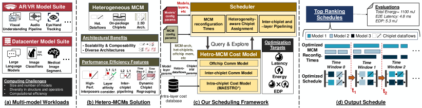
Figure 1: An overview of this work: (a) Emerging Multi-model workloads have introduced new challenges for AI hardware. (b) Heterogeneous MCMs present a promising solution to scale with multi-model workloads with some considerations. (c) Our proposed scheduling framework addresses said challenges to explore the heterogeneous scheduling space. (d) Provided Solutions provide optimized spatio-temporal scheduling strategies for the multi-model workloads.

Therefore, considering the new trend with multi-model AI workloads such as multi-tenancy [13, 56, 28] and AR/VR [27], we propose to explore heterogeneous chiplet-based MCM with AI accelerator chiplets with various dataflows to address the workload heterogeneity and concurrency. We consider inter-layer pipelining to enhance in-package data reuse and reduce offchip traffic. We formulate the scheduling problem and develop effective heuristics to navigate the huge scheduling space, whose problem scale is as big as O($10^{18}$) on a 6x6 chiplet MCM AI accelerator system even running a single model (BERT-L).

We evaluate five MCMs including three heterogeneous MCMs on ten multi-model scenarios: the first five scenarios are curated using MLPerf [46] to represent datacenter multi-tenancy scenarios. The models are selected based on recent datacenter model usage trends [13, 19] and the trend of large language model adoptions (e.g., GPT-L [44]), future-proofing emerging AI workloads such as AI assistant [35]. The other five scenarios are curated for AR/VR usage scenarios from XRBench as a practical use case for edge multi-model workloads  [27]. The evaluation results show the effectiveness of heterogeneous MCM combined with our scheduling method. Compared to the homogeneous MCM [48] running NVDLA [39] and Shi-diannao [8] style dataflows, heterogeneous MCM, on average, achieved 35.3% and 31.4% less energy-delay product (EDP) in each domain, respectively. Moreover, we performed ablation studies on the efficacy of our greedy scheduling algorithm, and found that it leads to superior multi-model schedules compared to other approaches, achieving 21.8% and 8.6% execution speedups and energy improvement on heterogeneous MCMs. We summarize our contributions as follows:

• We propose to explore heterogeneous dataflow MCM for emerging AI workloads with multiple models running concurrently for the first time.

• We formulate the MCM AI accelerator scheduling problem into a multi-tiered optimization problem to address intractably large scheduling space.

• Based on the formulation, we develop a scheduler that thoroughly considers heterogeneous MCM and multi-model workloads. The scheduler employs advanced scheduling techniques, such as inter-layer pipelining, dynamic chiplet regrouping utilizing latest representation such as the resource allocation tree [4].

• We codify our scheduling method and integrate it with a heterogeneous MCM AI accelerator cost model. We extend MAESTRO [24, 25] to model the latency and energy of MCM accelerators.

• We analyze the costs and benefits of heterogeneous dataflow MCM using future-proof multi-model workloads motivated by recent industry use cases and present the importance of the scheduling problem.

II Background

We discuss examples of emerging multi-model AI workloads and chiplet-based MCM AI accelerators.

II-A Multi-model AI Workloads

The success of AI algorithms in individual tasks (e.g., hand tracking, depth estimation, and speech recognition) led to the emergence of multi-model AI workloads, which include multi-tenant workloads at data centers [13, 56, 28] and real-time multi-model workloads such as AR/VR [27]. We summarize example multi-model AI workloads from industrial use cases in Table II. The models in such workloads are diverse in terms of the tasks and input modalities. For example, an industrial data center multi-tenant AI workload suite [13] includes a face recognition model based on support vector machine, recommendation models based on multi-layer perceptron, and a speech recognition model based on recurrent neural network (RNN). More recent workloads in data center AI workload include large language models [36], which adds more heterogeneity to the multi-model AI workloads. As discussed in prior works [26, 27], such multi-model workloads involve high heterogeneity in AI operators (or layers), which is one of the major challenges to accelerators that specialize the architecture and dataflow for a specific set of workloads.

II-B MCM AI Accelerators

Multi-chip Modules (MCM) comprise small functional dies (chiplets) that are packaged together to build a larger system. Chiplets are interconnected via on-package links typically through silicon interposer or organic substrates to create a network-on-package (NoP) [54, 20, 2]. A typical chiplet, in the context of a DNN accelerator, comprises off-chip memory, a global shared memory, and an array of processing elements connected via a Network-on-Chip (NoC) [6]. Advantages of the chiplet-based MCM architecture include the modularity and scalability to systems of varied scales simply by adjusting the number of chiplets placed on the package as well as low verification cost [38]. Based on such benefits, many chiplet-based MCMs have been developed for scalable DL inference [48, 5, 40, 51]. Such MCM accelerators successfully scaled up the systems up to 256 chiplets with 1 million processing engines  [40]. However, the effectiveness of a chiplet-based MCM system heavily depends on the careful distribution of computation amongst the different chiplets while balancing the added NoP/NoC communication costs.

II-C Scheduling space

As discussed in previous works [41, 26, 4], scheduling AI workloads on an accelerator can be considered as assigning a set of computations in various granularity (e.g., layer or compute tile) to each compute unit and ordering the computation. That is, the scheduling process is spatially and temporarily partitioning a workload onto a target accelerator architecture [4]. However, with that formulation, the scheduling space of multi-model workloads onto shared MCM accelerators is intractably large and high-dimensional, as discussed in Section I.

One approach to address the complexity is formulating the problem into multi-level decision problem where each decision subspace is a tractable problem [26, 6].We adopt a similar approach and formulate the multi-model workload scheduling on MCM as multiple-level decision problem, as shown in Figure 2. We discuss details of our problem formulation in detail and performance modeling methodology next.

III System Modeling and Problem Formulation

To develop a systematic approach to navigate complex scheduling space, we formulate the scheduling problem of the multi-model workloads running on a heterogeneous MCM AI accelerator.

III-A Base Formulation

To formulate the MCM scehduling problem, we first define multi-model workload scenario ($Sc$) and MCM hardware ($H$).

We formulate the workload in the granularity of layers in each model. Therefore, we formulate a multi-model workload scenario ($Sc$) as the collection of layers in the models included in the scenario. Letting the number of models included in $Sc$ as $|Sc|$ and the number of layers included in a model $m$ as $|m|$, we define $Sc$ as follows:

Definition 1.

Multi-model Workload Scenario (Sc)

$$Sc=\{layer_{i,j}|0<i\leq|Sc|,0<j\leq|m_{i}|\}$$

where $layer_{(i,j)}$ refers to the j-th layer of model i in Sc.

AI accelerator chiplets consist of a PE array, memory, and on-chip interconnection among memory and PEs. In addition to them, we also include the dataflow in the formulation to model heterogeneous chiplet MCM AI accelerator. Accordingly, we define an AI accelerator chiplet ($c$) as follows:

Definition 2.

AI Accelerator Chiplet (c)

$$c=\{df,N_{PE},BW_{noc},BW_{mem},Sz_{mem}\}$$

In Definition 2, $df$ refers to the dataflow, $N_{PE}$ is the number of PEs, $BW_{noc}$ is the NoC bandwidth, $BW_{mem}$ is the chiplet-level shared memory bandwidth, and $Sz_{mem}$ is the memory size in $c$.

Based on the definition of the chiplet, we formulate the MCM accelerator as the set of chiplets ($C=\{c_{1},c_{2},...,c_{N_{cpl}}\}$), NoP, and off-chip interface as follows:

Definition 3.

MCM AI Accelerator (H)

$$H=\{C,BW_{offchip},BW_{nop}\}$$

We assume the 2D mesh topology for NoP like Simba [48], and chiplets on two sides (left and right) of the packages have off-chip interfaces.

III-B Workload Partitioning Space

To reduce the complexity of the scheduling problem, we adopt a multi-level scheduling method, which splits the end-to-end workload defined in the layer granularity into coarse-grained layer groups, termed as the time window.  Figure 2 shows an example of the time window that contains six layers from Model A and five layers from Model B.

A time window ($tw$) is defined by the start time and the duration ($T_{S}$ and $T_{tw}$) and a set of assigned layers to the time window, as shown in Definition 4.

Definition 4.

Time Window (tw)
For a target workload scenario $Sc$, a time window $tw$ is defined as follows:

$$tw(Sc)=(T_{s},T_{tw},L)$$

where $L=\{l|l\in Sc\}$

The time window describes a set of layers to be executed on an MCM AI accelerator package, which is used for describing package level scheduling. For each chiplet, we define a finer-grained group of layers within a time window. We term the sub-set of layers within a time window as segment.

Definition 5.

Segment (sg)
For a time window $tw(Sc)$ and its layers $L(tw(Sc))$, the segment $sg(tw(Sc))$ is defined as follows:

$$sg(tw(Sc))=\{l|l\in L(tw(Sc))\}$$

To develop a systematic optimization algorithm for layer segmentation within each time window, we need to define the conditions of valid layer segments. We define the condition as follows:

Theorem 1.

The validity of segments in a time window
For a time window $tw(Sc)$ and its layers $L(tw(Sc))$, let the set of all segments for $tw(Sc)$ be $SG$, then $SG$ is valid if the following condition is satisfied:

$$\bigcup_{sg\in SG}sg=L(tw(Sc))\land\forall sg_{i}\neq sg_{j}\in SG,sg_{i}\cap sg_{j}=\emptyset$$

Theorem 1 states two conditions (1) the set of segments needs to cover all the layers in their time window for completing assigned layer computations for the time window and (2) all segments are exclusive to prevent redundant computing. The same idea extends to the time window as follows:

Theorem 2.

The validity of time window partitioning
For a multi-model workload $Sc$, its layers $L(Sc)$, and the set of time windows $TW(Sc)$, $TW(Sc)$ is valid if the following condition is satisfied:

$$\bigcup_{tw\in TW(Sc)}tw=L(Sc)\land\forall tw_{i}\neq tw_{j}\in TW(Sc),tw_{i}\cap tw_{j}=\emptyset$$

Both Theorem 1 and  Theorem 2 indicate that the time windows and segments need to be partitions of the workload and time window layer, respectively. Combining all definitions in this section, we formulate the workload partitioning space into the time window and segment as follows:

Definition 6.

Workload Partitioning Space
For a multi-model workload $Sc$, the time window partitioning space ($Sp_{tw}(Sc)$) and the layer segmentation space for a time window ($Sp_{sg}(tw)$) are defined as follows:

$$Sp_{tw}(Sc) =\mathbb{P}(L(Sc))$$

$$Sp_{sg}(tw) =\mathbb{P}(L(tw))$$

where $\mathbb{P}(A)$ refers to all possible partitioning of a set $A$

III-C Scheduling Space

A segment contains layers to be executed on a chiplet. Therefore, spatial (i.e., which segment runs on which chiplet) and temporal mappings (i.e., execution order of segments on each chiplet) of segments construct the scheduling space within each time window when segments are determined. Therefore, the scheduling space within a time window $tw(Sc)$ can be defined as follows:

Definition 7.

Scheduling Space in a Time Window ($SS_{TW}$)
For a given time window $tw(Sc)$ and a target MCM accelerator hardware $H$, the scheduling space within the time window ($SS_{TW}(tw(Sc),H)$ is defined as follows:

$$SS_{TW}(tw(Sc),SG,H)$$

$$\text{=}\{(sg,c,j)|sg\in SG\land c\in C_{H}\land j\in\mathbb{N}\land valid(sg,tw(Sc))\}$$

where $C_{H}$ refers to the set of chiplets in $H$ and val($sg$, $tw(Sc)$) indicates the validity of $sg$ for $tw(Sc)$

Each entry in $SS_{TW}$ describes the spatial and temporal mapping of a segment ($sg$). Spatial mapping can be defined as the target chiplet to execute $sg$. Accordingly, a target chiplet ($c$) is specified for $sg$. The temporal mapping is defined as the execution order. Therefore, a natural number $j$ is used to represent the execution order. Note that the execution order is defined separately on each chiplet. Based on Definition 7, we can define the entire scheduling space as the collection of that in each time window.

Definition 8.

MCM Scheduling Space for a Multi-model Workload ($SS_{Sc}(H)$)
For an MCM AI accelerator ($H$) and a multi-model workload ($Sc$), the scheduling space ($SS_{Sc}(H)$) is defined as follows:

$$SS_{Sc}(H)= \{(TW,SG_{TW},(SS_{TW}(tw,SG_{TW}(tw),H))|$$

$$TW\subset Sp_{tw}(Sc)\land SG_{TW}(tw)\subset Sp_{sg}(tw)$$

$$\land tw\in TW\}$$

where $SG_{TW}$ refers to the set of layer segments for each time window in $TW$

Definition 8 defines the entire scheduling space of an MCM AI accelerator for a multi-model workload as the cross-product of all possible time window partitioning, layer segmentation for each time window, and corresponding scheduling space within each time window.

III-D Scheduling Problem

Based on Definition 8, we define a schedule instance as the collection of spatial and temporal mapping for given valid time windows ($TW$) and segments for each time window ($SG_{TW}$).

Definition 9.

MCM Schedule
A schedule instance ($sched(Sc,H)$) is defined as follows:

$$sched(Sc,TW, SG_{TW},H)\text{=}\{(TW,SG_{TW},s)|valid(TW,Sc)$$

$$\land\forall tw\in TW:valid(SG_{TW}(tw),tw)$$

$$\land s\in SS_{TW}(tw,SG_{TW}(tw),H)\}$$

where $SG_{TW}$ refers to the set of layer segments for each time window in $TW$

Using Definition 9, we formulate the scheduling problem as a minimization problem of an optimization metric of choice (e.g., latency and energy), as follows:

Definition 10.

MCM Scheduling Problem

$$\operatorname*{argmin}_{TW,SG_{TW},Sched}OptMetric(TW,SG_{TW},Sched,H)$$

where $Sched=sched(Sc,TW,SG_{TW},H)$

The optimization metric can be chosen by users depending on the use case. In our scheduler, we adopt a comprehensive and customizable score that thoroughly consider all of latency, energy, and energy-delay product (EDP), allowing users to configure their own optimization metrics, which can the mentioned frequently used metrics or a user-defined function that takes a schedule instance and generates a custom metric.

III-E Latency Modeling

To develop a scheduler based on the scheduling problem formulation in Section III-C, we need to be able to evaluate each schedule on target MCM AI accelerator hardware. For that, we extend MAESTRO [24] to the chiplet domain and model the latency of MCM AI accelerators concurrently executing multi-model workloads on a shared MCM system in a bottom-up fashion. We discuss our latency evaluation methodology in detail, focusing on our extension for the MCM and multi-model workloads.

Layer Latency. The latency incurred by an individual layer, $l$, mapped onto an accelerator chiplet is defined as:

$$Lat(l)=Lat^{ip\_com}(l)+Lat^{comp}(l)+Lat^{op\_com}(l)$$

$Lat^{comp}(l)$ being the layer computation cost dependent on the AI accelerator chiplet parameters Definition 2; $Lat^{ip\_com}(l)$ is latency incurred from loading the layer operands (input activations and weights), and $Lat^{op\_com}(l)$ from transmitting the output activation to a subsequent layer. As for $Lat^{com}$, it is defined as:

$$\small Lat^{com}=\begin{cases}0,\text{if same chiplet}\\ \frac{Sz_{data}}{BW_{nop}}+n_{hops}\times Lat_{hop}+\delta,\text{if same package}\\ \frac{Sz_{data}}{BW_{mem}}+n_{hops}\;\text{x}\;Lat_{hop}+Lat_{mem}+\delta,\text{if offhcip}\end{cases}$$

where assuming sufficient memory for double-buffering on each chiplet accelerator, communication costs become incurred when transmitting data to/from another chiplet on package or the offchip memory. The first term $\frac{Sz_{data}}{BW}$ reflects transmission latency; the second term is captures propagation latency across $n_{hops}$ between the source and destination; $\delta$ is an additional latency term for potential NoP traffic conflicts; $Lat_{mem}$ is the cost from read/write access of data at the offchip memory.

Time Window Latency. We first model a layer segment’s latency in a time window as follows:

$$Lat(sg)=\sum_{n=1}^{N}Lat^{comp}(l_{n})+Lat^{ip\_com}(sg)+Lat^{op\_com}(sg)$$

The first term represents the sum of individual layer computational latencies; $Lat^{ip\_com}$ is the initial external data transfer loading costs of necessary off-chiplet input activation and parameter weights; $Lat^{op\_com}$ is the transmission latency from transmitting segment output data to the next segment or writing back to memory.

Based on the segment’s latency, the time window latency can be defined as:

$$Lat(tw)=\max\limits_{SG_{m}\subset SG}\begin{cases}\sum_{sg_{k}\in SG_{m}}Lat(sg_{k}),\hfill\text{if end-to-end}\\ \max\limits_{sg_{k}\in SG_{m}}Lat(sg_{k}),\hfill\text{if pipelining}\end{cases}$$

where $SG_{m}$ represents the set of segments in a time window associated with a model $m$. The latency of $SG_{m}$ can either be the maximum out of all $m$ segments if pipelining or their summation in the base case. The latency of the entire window is the max out of all $SG_{m}\subset SG$.

Overall Latency. The overall Scenario latency can then be estimated as the aggregate across all time windows:

$$Lat(Sc)=\sum_{tw_{j}\in TW}Lat(tw_{j})$$

III-F Energy Modeling

Albeit similar to latency, Energy costs are always aggregated. The base communication energy cost is defined as:

$$E^{com}=\begin{cases}0,\hfill\text{if same chiplet}\\ Sz_{data}\times E_{tx\_bit}\times n_{hops},\hfill\;\;\text{if same package}\\ Sz_{data}\times E_{tx\_bit}\times n_{hops}+E_{mem},\;\hfill\text{if offchip}\end{cases}$$

where the energy incurred from moving data across the package is equal to the product of data size, number of hops, and the per-bit transmission energy ($E_{tx\_bit}$). In case of an offchip data transmission, the cost of memory access $E_{mem}$ is added.

The overall energy consumption across the entire time windows can be computed as the sum of energies of its constituent components as follows:

$$E(l) =E^{ip\_com}(l)+E^{comp}(l)+E^{op\_com}(l)$$

$$E(tw) =\sum_{sg_{k}\in SG}E(sg_{k}),\;\;\;E(Sc)=\sum_{tw_{j}\in TW}E(tw_{j})$$

IV Scheduling Framework

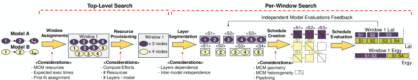
Figure 2: An overview of our scheduling algorithm.

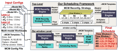
Figure 3: Our proposed multi-model scheduling framework on heterog. MCM.

We discuss our scheduling framework for multi-model workloads on heterogeneous MCMs based on the hierarchical search space characterization and problem formulation in Section III. As illustrated in Figure 2, our scheduling algorithm is a two-level approach: top-level and per-window searches. Top-level search is responsible for selecting layers in each model to be scheduled within a time window and determining the initial number of chiplet nodes for each model. Per-window search explores the spatial and temporal partitioning (i.e. tiles or layer segments) of the layers in each model at the chiplet granularity. To explore the chiplet granularity tiling space, we generate valid inter-chiplet-pipelined schedules utilizing a scheduling tree structure inspired by the RA Tree [4]. Each schedule is evaluated using our custom heterogeneous MCM cost model which provides feedback to the chiplet level tiling (”layer segmentation” in  Figure 2) with expected metrics (latency, energy, EDP, etc.).

We codify our scheduling algorithm into a software framework, as illustrated in Figure 3. As inputs, our scheduling framework receives (1) description files of the multi-model workloads (layer parameters, topology, dependencies, etc.) and (2) a description file of the MCM hardware specification, such as the number of chiplets, the shape, and dataflow organization of the chiplet arrays, NoP bandwidth, on-chiplet memory size, and so on. As outputs, our scheduling framework reports an optimized schedule with expected metrics such as latency, energy, EDP, or other user-defined metrics as a combination of latency and energy. Our scheduling framework consists of four software engines, which handle each step of the scheduler discussed in this section. Each engine is responsible for each step of our two-level scheduling method as illustrated in Figure 2. We discuss each engine and our cost model utilized by the framework next.

IV-A MCM Reconfiguration Engine (MCM-Reconfig)

The MCM-Reconfig engine at the top-level step receives the multi-model workload descriptions with layer information in each model, layer dependency, and expected latency and energy of each layer on each chiplet class offline-analyzed by MAESTRO [24]. The MCM-Reconfig engine is responsible for the window assignment in Figure 2, which (1) generates candidate time window partitioning strategies via sampling a set of discrete points in time reflecting the boundary points between execution windows and (2) assigns layers from models to each time window. As the final assignment of layers to chiplets is not yet known, the decisions in MCM-Reconfig engine are based on expected execution times. Formally, given $|DF|$ dataflow style classes, the expected execution latency for a layer $l$ is:

$$\mathbb{E}(Lat(l))=\sum_{i=1}^{|DF|}\frac{n_{df_{i}}}{|\mathcal{C}|}\times Lat(l\rightarrow i)$$ (1)

where $n_{df_{i}}$ indicates the number of class $i$ chiplets integrated onto the MCM having $|C|$ chiplets in total; $Lat_{l\rightarrow i}$ is layer $l$ latency when scheduled on the class $i$ chiplet, which is retrieved offline from latency database generated by MAESTRO [25, 24]. The average execution time information is utilized in MCM-Reconfig engine for window assignment process illustrated in Figure 2.

Time Windows Characterization. MCM-Reconfig engine first specifies the number of windows, which is the coarse-grained scheduling granularity in our scheduling algorithm. We define $n_{splits}$ as a user-defined parameter to characterize the number of time windows and explore proper cut points for each model. For example, in Figure 2, the model A has a cut after layer 6, which led to having layers 1-6 in Window 1. The worst-case latency experienced by a model in the multi-model workload is set as the time horizon which we partition into periodic time windows.

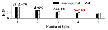
Figure 4: Comparing top configurations from our periodic windowing against layer-optimal using GPT2-L and UNet models. $\Delta$ indicates the $\%$ difference.

Greedy Layer Packing Algorithm. Multi-model workload introduces a challenge: the time window boundary determined by the cut points of one model might not be aligned with other models. Therefore, we adopt a first-fit greedy-packing heuristic where layers are assigned to an execution window if their execution time is expected to be within a time window (see Algorithm 1), even if the start and finish time is not aligned with those of a time window. Any layer with execution time lies across two time windows is deferred to the next time window. This approach not only solves the time window - layer execution time misalignment problem, but also facilitates (i) running low-latency layers in earlier windows, preventing starvation of small workloads blocked by heavy workloads. (ii) Dynamically controlling number of time windows when needed by skipping trivial windows without any workloads.

Using a small multi-model workload entailing UNet [47] and GPT-L [44] from Table II, we analyzed the efficacy of our periodic window characterization with first-fit greedy packing against a layer-optimal approach that considers every possible layer from the workloads as a potential cut point. In Figure 4, run our full scheduling algorithm and compare the top two scheduling choices with minimal EDP. We observe the $\%$ performance difference ($\Delta$) in EDP values between the two strategies increase with a rising number of splits. However, the overall rate of EDP improvement starts to stagnate after 4 splits. Based on this analysis, we set $n_{splits}$=4 (5 time windows) as our default unless otherwise stated. Further ablation is performed in the evaluation Section V.

Algorithm 1 Greedy Layer Packing Algorithm

1:$M$ (workloads), $\mathcal{T}$, $\mathcal{C}$, $DF$

2:$L2W$ (Layer(s) to windows assignments)

3:Function LayerAssignment($M$, $\mathcal{C}$, $\mathcal{T}$)

4:  for $m\in M$ do

5:   $exec\_win=()$

6:   $win\_idx,used\_cycles=0,0$

7:   for $l\in m$ do

8:    $\mathbb{E}(Lat(l))=\sum_{i=1}^{|DF|}\frac{n_{df_{i}}}{|\mathcal{C}|}\times Lat(l\rightarrow i)$

9:    while True do

10:     if $win\_idx==|\mathcal{T}|$ then

11:      $Slack$ = $None$

12:     else

13:      $Slack$ = $\rho[win\_idx]-used\_cycles$      

14:     if $Slack$ == $None$ or $\mathbb{E}(Lat(l))<=Slack$ then

15:      $exec\_win$ += $(l,)$

16:      $used\_cycles$ += $\mathbb{E}(Lat(l))$

17:      Break

18:     else

19:      $L2W[win\_idx][m]=exec\_win$

20:      $used\_cycles=\mathcal{T}[win\_idx]$

21:      $exec\_win=()$

22:      $win\_idx$ += 1          

23:    $L2W[win\_idx][m]=exec\_win$      

IV-B Provisioner Engine (PROV)

The PROV engine is responsible for providing an initial estimate on the number of chiplet needed by each model workload in every time window given a candidate partitioning strategy. This assignment is agnostic to the underlying chiplets’ resources or dataflow, and hence we refer to chiplet resources in this state as nodes. We implement our PROV engine for nodes’ distribution across various model workloads using a set of rules. The rules are based on expected latency, energy, EDP, or user-defined metric for each corresponding window. This computational effort is associated with a specified performance optimization goal, denoted as $\mathcal{P}$ where $\mathcal{P}\in\{Lat,Ergy,EDP\}$, Following a uniform distribution rule, the number of nodes $N_{i}$ allocated to the $i^{th}$ model is:

$$N_{i}=round(\frac{\mathbb{E}(\mathcal{P}_{i})}{\sum_{j}(\mathbb{E}(\mathcal{P}_{j})}\times|\mathcal{C}|)$$ (2)

where $\mathbb{E}(\mathcal{P}_{i})$ represents the expected value of the performance optimization goal for model, computed in a manner similar to the expected execution latency formula in Equation (1), whereas the sum term in the denominator represents the sum of all expected values for every model workload in the current time window. Though in principle other allocation strategies can be implemented for the Provisioner, the benefits of having a rule-based Provisioner as such are twofold:

• The Provisioner becomes specialized in warranting a fair spatial distribution of resources per window across the various model workloads, leaving temporal allocation tasks to be handled through the other engines.

• Circumventing an additional top-level search space specification with a high degree of uncertainty, acting instead as a regulator mid-way throughout the framework without aggravating the search complexity.

To ensure the progression of all model workloads assigned to a window, we enforce the allocation of at least one resource per model per window to account for rounding errors in Equation (2) when a model workload assigned to the window has negligible computational overhead compared to its peers. The reallocation process iteratively reassigns nodes from models with max number of resources until the constraint is satisfied.

IV-C Segmentation Engine (SEG)

As the first module in the per-window level, the SEG module is instantiated for every time window, receiving topologically sorted sets of layers from each model to be further partitioned into segments. Segmentation is the process of partitioning a set of layers into smaller subsets of layers (i.e., segments or tiles) that can be mapped to a computing resource for exclusive execution throughout the duration of a time window. Different segmentation choices reflect various trade-off points between the layer-sequential and layer-pipelining execution features: the former controls the granularity of layers within each segment to be co-located for sequential execution on a single chiplet resource; the latter exploits inter-layer and -chiplet pipelining opportunities between various segments.

Segmentation Search Space. As per our formulation in Section III, a segmentation candidate is represented by a sequence of splitting points, where candidate splitting points are specified after each layer for each model’s set of layers provided to the SEG Given $|L_{i}|$ and $|N_{i}|$ as the respective number of layers and number of assigned nodes (from PROV) for a model workload $m_{i}$, the max number of segments that can be generated for $m_{i}$ becomes upper bounded by $N_{i}$. Hence, the overall segmentation space complexity is $\mathcal{O}(\Pi_{i}\ |L_{i}|\times{|N_{i}|})$, with the $\Pi_{i}$ indicating the combinatorial space across all models. To aid in managing the rising multi-model segmentation space complexity, we introduce the following heuristics.

Heuristic 1. Product to summation reduction. We enable SEG to navigate the segmentation search space with reduced complexity through a two-step process: (1) SEG leverages the independence of segments from different models to initially explore the segmentation subspace for each model separately (2) Segmentation point candidates from the top-k configurations for each model are used to construct a smaller search space for the combinatorial co-exploration of the segmentation space. Through this heuristic, a sizable reduction in the search space complexity can be realized from $\mathcal{O}(\Pi_{i}\ |L_{i}|\times{|N_{i}|})$ down to $\mathcal{O}(max(|L_{i}|\times{|N_{i}|}))$.

Heuristic 2. Node allocation constraint. We designate an additional user-specified constraint to restrict the number of nodes provisioned to a model within a window based on its number of layers. The constraint is particularly beneficial in cases where there is mismatch between the multi-models’ distribution of computational efforts across their respective layers. For instance, a scenario may arise where a single compute-intensive layer may be assigned to same window alongside dozens of layers from smaller models, leading to an unnecessary explosion in the segmentation search space. The enforcement of this constraint is performed by the PROV.

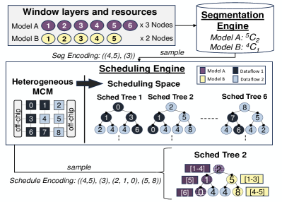
Figure 5: Schedules creation through the SEG and SCHED engines.

IV-D Scheduling Engine (SCHED)

The innermost Scheduling engine (SCHED) is responsible for generating the final mapping of layer segments to the physical chiplet accelerators on the target MCM.

Scheduling Search Space. As illustrated in Figure 5, the scheduling search space for the mapping of $M$ model workloads onto $\mathcal{C}$ chiplets can be represented as a forest of scheduling trees. Throughout this sub-section, we use three terms to describe different parts of the scheduling search space: (i) forest; as the entire collection of search trees. (ii) tree; characterizing a single scheduling tree modeling with all the $M$ models involved. (iii) subtree; representing a subset part of each tree exclusively associated with a model $m_{i}\in M$.

Scheduling Tree Composition. every node in a scheduling tree corresponds to a unique chiplet resource on the MCM showcasing its distinctive heterogeneous features (i.e., dataflow). Each chiplet is assigned a unique identifier based on a row-major order traversal across the MCM grid. Tree edges are constructed based on each chiplet’s XY neighbors connected directly through an interposer. Though a node $j$ can be replicated throughout the tree, it can only be visited once, indicating its exclusive occupancy by a model.

Trees Distinction. within each tree, the root nodes of the subtrees specify different chiplets as potential starting positions for candidate model schedules. This is particularly relevant when the underlying pattern of heterogeneity is non-uniform, causing scheduling options to be dependent on the starting position (see Figure 5). Thus, the scheduling space coverage starts by selecting a tree, represented by a permutation sequence of subtrees’ root nodes – e.g., permutation sequence [i,j,k] indicates exploring scheduling candidates for a tree with scheduling candidates starting at chiplet positions $i$, $j$, and $k$ for a 3-model workload. The depth of model $i$’s subtree is determined by its number of provisioned resources $N_{i}$.

Candidate Schedules Generation. Through traversing each subtree, we can obtain candidate execution schedules for each model by assigning segments orderly to the subtree’s nodes. Starting from the root node of the first model’s subtree, a constrained depth first search (DFS) is performed generating a candidate schedule path once the full subtree depth ($N_{i}$) has been reached. This traversal is repeated for each subsequent subtree, constrained on the preceding subtree’s prior visited nodes. Traversal paths from each subtree are then aggregated to form the overall scheduling candidate.

Encoding and Search Algorithm. As shown in Figure 5, use a $2\times|M|$-length tuple to represent the final scheduling encoding, where the first $M$ entries reflect segmentation decisions for each model $m_{i}$, and the latter $|M|$ entries reflect schedule mappings of segments to chiplets for each workload. This form of encoding facilitates supports having different search algorithms for each engine. We tested both brute-force and evolutionary algorithms as will be shown in Section V.

Schedules Starting Positions. We constrain the number of scheduling trees to chiplet nodes that satisfy either of the following two conditions: (i) chiplets that maintain a direct link to an offchip DRAM memory interface (as in the right and left-most chiplets of the MCM in Figure 5). (ii) ending chiplet positions from the preceding window, which enable leveraging data locality across time windows.

Search Space Complexity. Given $|M|$ as the number of models in a given window, $|T|$ the number of scheduling trees in the search space, $d$ is a traversal path’s degree of freedom, and $N_{max}$ representing the max number of resources allocated to any model in this window. The scheduling search complexity can be given by $\mathcal{O}(|M|\times|T|\times d^{N_{max}})$.

IV-E Cost Model and Scoring

TABLE I: MCM microarchitecture parameters from [48, 40]. All numbers are scaled to 28 nm process node technology.

Offchip Memory	DRAM latency	200 ns
	DRAM energy	14.8 pJ/bit
	DRAM bandwidth	64 GB/s
Package	NoP intercon. latency	35 ns/hop
	NoP intercon. energy	2.04 pJ/bit
	NoP intercon. bandwidth	100 GB/s/Chiplet

We implement a cost model for evaluating scheduling candidates on different performance efficiency metrics.

Cost Model. The overall cost model constitutes three distinctive cost model components: offchip communication model, inter-chiplet communication model, and intra-chiplet cost model. We follow our latency and energy modeling characterization in Section III-E and Section III-F, and use the architectural parameters provided in [48, 40] for the offchip and inter-chiplet communication costs as shown in Table I. For the intra-chiplet cost model, we utilize the open-source accelerator cost model, MAESTRO [24, 25], to evaluate intra-chiplet performance based on a chiplet’s underlying dataflow and hardware parameters.

Scoring. Scores are estimated based on latency, energy, or EDP metrics following Section III modeling. The SCHED aggreages scores for each model’s schedule, and returns the top performing configuration to the SEG engine to rank segmentation strategies. Top segmentation strategies in each window are aggregated to score the overall scheduling strategy at MCM-Reconfig (see the scoring flow in Figure 3).

V Evaluation

V-A Experimental Settings

TABLE II: Our experimental Multi-model workload scenarios for datacenter and AR/VR use-cases inspired by MLPerf [46, 37] and XRbench [27] benchmarks. ‘sl’ indicates sequence length

Use-Case	Scenario	Models	Batch Size
Datacenter (MLPerf) [46, 37]	(1) LMs	GPT-L [44] (sl=128)	1
		BERT-L [7] (sl=128)	3
	(2) LMs + Image (light)	GPT-L [44] (sl=128)	1
		BERT-L [7] (sl=128)	3
		ResNet-50 [14] (224$\times$224$\times$3)	1
	(3) LMs + Image (heavy)	GPT-L [44] (sl=128)	1
		BERT-L [7] (sl=128)	3
		ResNet-50 [14] (224$\times$224$\times$3)	32
	(4) LMs + Segmentation + Image (heavy)	GPT-L [44] (sl=128)	8
		BERT-L [7] (sl=128)	24
		U-Net [47] (512$\times$512$\times$1)	1
		ResNet-50 [14] (224$\times$224$\times$3)	32
	(5) LMs + Segmentation + Image (heavy)	GPT-L [44] (sl=128)	8
		BERT-L [7] (sl=128)	24
		BERT-base [7] (sl=128)	24
		U-Net [47] (512$\times$512$\times$1)	1
		ResNet-50 [14] (224$\times$224$\times$3)	32
		GoogleNet [50] (224$\times$224$\times$3)	32
AR/VR (XRBench) [27]	(6) AR Assistant	D2GO [34] (Object Det.)	10
		PlaneRCNN [29] (Plane Det.)	15
		MiDaS [45] (Depth Est.)	30
		Emformer [49] (Speech Rec.)	3
		HRViT [9] (Semantic Seg.)	10
	(7) AR Gaming	PlaneRCNN [29] (Plane Det.)	15
		Hand S/P [11] (Hand Track.)	45
		MiDaS [45] (Depth Est.)	30
	(8) Outdoors	D2GO [34] (Object Det.)	30
		Emformer [49] (Speech Rec.)	3
	(9) Social	EyeCod [59] (Gaze Est.)	60
		Hand S/P [11] (Hand Track.)	30
		Sp2Dense [32] (Depth Ref.)	30
	(10) VR Gaming	EyeCod [59] (Gaze Est.)	60
		Hand S/P [11] (Hand Track.)	45

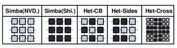
Figure 6: The evaluated MCM chiplet organizations.

Multi-Model Workloads. Our evaluations are performed on multi-model workload scenarios based on models from (i) MLPerf inference benchmark [46, 37] for the datacenter multi-tenancy setting; (2) XRBench [27] for AR/VR workloads. The full list of scenarios is provided in Table II covering a wide range of use-cases with varying degrees of diversity and complexity. We implement our MLPerf following datacenter usage trends in [13, 42, 19].

MCM System. We follow Simba’s on-package chiplet arrangement to implement our MCM experimental templates [48]. Simba comprises a total of 36 chiplets connected through a Mesh topology and arranged as four $3\times 3$ groups of chiplets. We implement (1) $3\times 3$, and (2) $6\times 6$ MCM templates for our experiments. For each, we adopt XY routing for on-pacakge data movement, and integrate further memory interfaces on the sides of the outer chiplets, providing direct links to the offchip DRAM via double-sided memory channels as in [10]. We consider 4096 PEs/chiplet and 256 PEs/chiplet for the datacenter and AR/VR settings, respectively. We set the L2 shared memory size in each chiplet to 10 MB, inspired by the on-chip memory size in a recent mobile accelerator [43].

Baselines and Heterogeneity Patterns. We choose Shi-diannao [8] and NVDLA [39] dataflow styles for our accelerator chiplets. We accordingly implement two baselines:

• Standalone. Each model in a multi-model workload is assigned a single chiplet for execution, all chiplets posses the same dataflow.

• Simba-like Pipelining. In each time window, Model workloads can be assigned to more than one chiplet to leverage pipelining benefits. All chiplets posses the same dataflow.

We implement several patterns for the heterogeneous on-package integration of Shi-diannao and NVDLA chiplet accelerators. As shown in Figure 6, we test heterogeneous checkerboard, sides, and cross patterns.

Optimization Targets. We perform our search space exploration experiments to target optimizing a single metric at a time, coining the terms Latency Search, Energy Search, and EDP Search. EDP Search is our default experiment.

Search Algorithms and Evaluation. We adopt a brute-force search for all experiments entailing the $3\times 3$ MCM template. For the scaled $6\times 6$ experiment, we implement an evolutionary algorithm for the SEG module as a meta-heuristic approach to navigate the rising complexity. We set the population size and max number of generations to 10 and 4, respectively. The evaluation criteria follows the scoring function based on hierarchical latency and energy models derived in Section III.

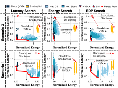
Figure 7: Comparing brute force scheduling space exploration processes across various MCM configurations for various search targets for scenarios 4 and 5 from Table II. standalone Shi-diannao and standalone NVDLA indicate cases where execution is performed on a single chiplet supporting said dataflow.

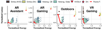
Figure 8: Pareto optimal results on the EDP search experiments for the labeled XRBench usage scenarios. Results normalized by standalone NVDLA

V-B Search Space Exploration Analysis

We compare the $3\times 3$ MCM brute-force search experiments for the heterogeneous and baseline configurations across the different optimization targets for the datacenter and AR/VR usage scenarios. All evaluations are normalized by the standalone NVDLA baseline. Though we performed experiments for all use-cases listed in Table II, we focues our analysis on a subset of experiments in Figures 7 and 8 due to space limitations: Scenarios 3 and 4 from the datacenter use cases, and the AR Gaming, Outdoors, and VR gaming scenarios from the AR/VR use-cases.

Pipelining Speedups. We observe that the combination of pipelining and chiplet heterogeneity lead to Pareto-optimal operating points that offer performance improvement opportunities. In Figure 7, we see that pipelining individually can offer speedups over standalone baselines. For example, Scenario 3 (Latency Search) – top-left most sub-Figure – shows Simba (NVDLA) realizing configurations achieving up to 4$\times$ speedup over the standalone NVDLA. This results from potential multiple chiplet assignments per window to each model, speeding up compute-intensive layers of GPT-L,BERT-L, and the 32-batch ResNet-50 models.
Heterogeneous Integration Synergy. As the density of multi-model workloads increase (Scenario 4 from Figure 7), we observe the effectiveness of homogeneous pipelining drops due to the increased competition for chiplet resources from heavier workloads. Heterogeneous MCM solutions become viable in such cases as they add another dimension for boosting performance through heterogeneous pipelining schedules, which compensate for the rising complexity through considering the varying affinities of diverse model layers, improving both latency and energy efficiency as seen in their respective search experiments. This benefits of heterogeneous pipelining also hold for the AR/VR scenarios as seen by up to $1.25\times$ execution speedups in Figure 8.
Model Suite Diversity. The degree of diversity within the multi-model use-case also influences the overall performance improvement. In Scenario 3 (Figure 7 top), GPT-L and BERT-L were dominant transformer-based workloads with strong affinities towards the NVDLA dataflow style, contributing to the homogeneous Simba (NVDLA) solutions dominating the Pareto frontier. Scenario 4 (Figure 7 bot) and the AR/VR (Figure 8), more diversification of the layer workloads set lead more heterogeneous pipelining solutions to dominate the Pareto frontier.
Target Optimization. As illustrated in Figure 7, the dominance of MCM configurations is also dependent on the target optimization metric. For instance in Figure 7 Scenario 4, the Standalone NVDLA baseline is the most energy-efficient solution as it does not incur NoP data movement costs from pipelining. However for Energy Search experiment, Het-Sides configuration identifies scheduling solutions that become the most energy efficient ones by leveraging heterogeneity to overcome extra NoP costs.

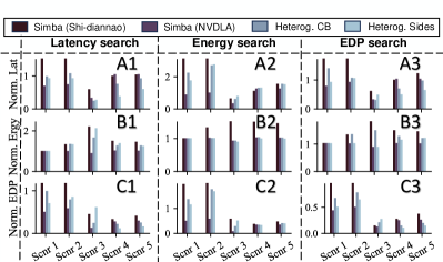
Figure 9: Comparing latency, energy, and EDP evaluations for the top-scoring candidates from every search experiment with different optimization criteria across every scenario in Table II. Values normalized by NVDLA standalone.

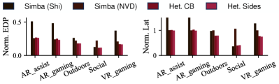
Figure 10: EDP and Latency comparison for the AR/VR usage scenario on various MCM templates for the EDP search experiment.

V-C Top Performing Schedules Comparison

We compare the top-performing scheduling configurations for each MCM configuration across the various scenarios.

NoP and Inter-chiplet Pipelining. We take barplot A1 in Figure 9 as an example and and zoom in on the Simba (NVDLA) configuration (2nd category) in each scenario. In Scenarios 1-3, the small number of models and limited diversity lead the benefits of inter-chiplet pipelining to outweigh the added NoP costs, enhancing throughput and achieving latency speedups over the standalone NVDLA baseline reaching $1.4\times$, $1.4\times$, $3.3\times$, respectively. Scenarios 4 and 5 sustain larger NoP overheads due to the increased traffic contention from more workloads, causing Simba (NVDLA) $1.05\times$ slowdown compared to the baseline in both scenarios.

Heterogeneity Pattern Choices. Across the heterogeneous MCM scheduling options in Figure 9 (Het-CB and Het-Sides), we notice that in the majority of cases, Het-Sides outperforms Het-CB. The reason being is that Het-Sides presents workloads with inter-chiplet pipelining options that can either be homogeneous or heterogeneous based on the chiplets heterogeneous arrangement . This is especially beneficial in cases where are sequences of layers that can benefit from pipelining while sharing the same dataflow affinities, unlike Het-CB which can only offer the heterogeneous pipelining option.

Scenario and Optimization Target. In all matching criteria plots (A1, B2, and C3), Het-Sides configuration at the most compute-intensive and diverse scenarios 4 and 5 consistently outperforms all baselines. For example, Scenario 4 EDP in barplot C3 is reduced by factors of 2.3$\times$ and 2.6$\times$ compared to Simba (NVDLA) and Simba (Shi-diannao), respectively, while being 9.25$\times$ less than the standalone NVDLA. We also show in Figure 10 the matching EDP barplot for the AR/VR experiments. We observe that Het-Sides option remains the most efficient option compared to the Simba baselines, achieving on average $5.2\%$ improvement over the standalone NVDLA.

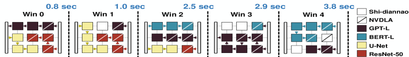
Figure 11: Illustration of the top-scoring partitioning strategy for the scenario 4 experiments given the heterogeneous-sides configuration. Each window showcases the top-performing schedule within, and the mapping of models onto chiplets. Time boundaries between successive windows are computed over 500 MHz.

Het-Sides Top Scheduling Strategy. In Figure 11, we illustrate the overall scheduling strategy for the top-scoring Het-Sides solution from the EDP search in Scenario 4. The Figure depicts the per-window inner schedules and the progression of accumulative latency for processing the workloads packed into each window. The distinguishing feat from this top scheduling strategy is the non-uniformity of time windows resulting from the greedy-packing heuristic, where smaller workloads (ResNet-50) are assigned to the earlier windows at the expense of larger workloads (e.g., from BERT-L) being delayed to subsequent windows. This facilitates (i) optimizing the schedules of smaller workloads at a finer level of granularity; (ii) avoiding starvation of smaller workloads. Starting from window 2, GPT-L and BERT workloads dominate the schedule, having their segmentation and mapping strategies optimized to minimize the experienced EDP in each window. In Table III, we breakdown how the latency of each window is estimated alongside their assigned number of layers.

TABLE III: End-to-end latency breakdown in seconds for the top partitioning candidate in Figure 11. ‘Ideal‘ indicates individual model latencies unconditioned on window times.

	W0	W1	W2	W3	W4	ideal	tot	#layers
GPT-L	0.23	0.21	1.02	0.28	0.23	1.97	3.1	120
BERT-L	0	0	1.47	0.4	0.90	2.77	3.76	60
U-Net	0.21	0.14	0.46	0	0	0.8	1.45	23
ResNet	0.78	0.17	0.11	0	0	1.1	1.1	66
Window	0.78	0.21	1.47	0.4	0.9	-	3.8	269
$\#$layers	60	30	131	25	23	-	-

V-D Ablation on Windowing and Chiplets Scaling

Ablation Study on Time Partitioning. Using Scenario 4 and Het-Sides EDP Search experiments, we study how performance changes when varying $n_{splits}$ and repeating the experiment in Figure 12. We observe the rate of EDP improvements starts to plateau after $n_{splits}$=4 similar to our analysis in Figure 4, where EDP of the top candidate is reduced from $n_{splits}$=4 to $n_{splits}$=5 by a factor of 1.04$\times$.

Ablation on Greedy Packing Algorithm. Using Scenario 4 and Het-Sides configuration, We tested the efficacy of our first-fit greedy layer packing algorithm against a uniform packing baseline, which uniformly distributes layers from each model across time windows in a uniform fashion. The Greedy layer packing algorithm was superior, improving execution speedups and energy efficiency by 21.8% and 8.6%, respectively.

Scalability. We assess the scalability of our search framework using the full 6$\times$6 Simba MCM system, where we implement an evolutionary algorithm for the SEG considering the rising problem complexity from the inclusion of more chiplets. We perform the search for our default experimental settings and Scenario 4 given $n_{splits}\in\{2,3\}$. We employ a Heterog-Cross pattern and compare it against the Simba baselines in Figure 13. We find that the Heterog-Cross top-scoring schedule outperforms those from the Simba baselines in all cases across all metrics. At $n_{splits}$=3, Heterog-Cross leads to 2.3$\times$ and 1.9 $\times$ reduction in EDP; 2.1$\times$ and 1.8$\times$ reduction in latency; over Simba (Shi-diannao) and Simba (NVDLA) and, respectively.

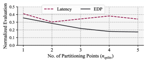
Figure 12: Sweep of $n_{splits}$ for the $3\times 3$ Heterog-Sides MCM configuration under EDP search showing EDP and latency results for each case’s top choice.

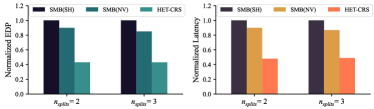
Figure 13: Comparing EDP and Latency at $n_{splits}\in\{2,3\}$ for the $6\times 6$ MCM for target EDP optimizaiton and an evolutionary search algorithm.

VI Related Works

Scheduler for Accelerators. Table IV compares our work against prior scheduling works. As shown, the related works can be categorized into two groups: one which has considered aspects of inter-layer pipelining and chiplet-based systems [48, 10, 52, 4, 5], while the other category of works focused on multi-model workloads on heterogeneous platforms [26, 22, 12, 30, 23]. Only this work addressed MCM, multi-model workloads, inter-layer pipelining, and heterogeneous dataflow.

Multi-chiplet Modules. Several works have proposed to address the performance scalability challenge for high-performance computing and DNN acceleration via MCM integration [48, 18, 40, 52, 1]. Simba [48] is one notable workload which pioneered a scalable deep learning inference accelerator employing MCM integration leveraging non-uniform work partitioning, communication-aware data placement, and cross-layer pipelining.

Intra- and Inter-layer Parallelism. Numerous works have explored intra-layer parallelism to maximize performance efficiency and resource utilization by partitioning DNN layers into smaller parallelizable tiles [41, 15, 17, 31, 58, 57, 16]. Other works have studied the inter-layer scheduling space to compensate for workloads characterized by low degrees of parallelism [10, 21, 33, 60, 4].

TABLE IV: Comparison against prior related scheduling works.

Work	Chiplet-based	Multi-	Inter-Layer	Heterog-
	Systems	Models	Pipelining	Aware
Simba[48]	✓		✓
Tangram[10]			✓
NN-baton[52]	✓
SET[4]			✓
Gemini[5]	✓		✓
Herald[26]		✓		✓
MAGMA[22]		✓		✓
Planaria[12]		✓		✓
Veltair[30]		✓
MoCA [23]		✓
This Work	✓	✓	✓	✓

VII Conclusion

In this work, we explored the scheduling space of a new class of MCM accelerator architecture, heterogeneous MCM AI accelerator, targeting multi-model AI workloads. We identify that the scheduling problem is intractably large but multi-level problem formulation and heuristics we proposed are effective for the extended scheduling problem. The results also show that heterogeneous MCM accelerator is beneficial multi-model workloads, which motivates further exploration.

References

- [1] Akhil Arunkumar, Evgeny Bolotin, Benjamin Cho, Ugljesa Milic, Eiman Ebrahimi, Oreste Villa, Aamer Jaleel, Carole-Jean Wu, and David Nellans. Mcm-gpu: Multi-chip-module gpus for continued performance scalability. ACM SIGARCH Computer Architecture News, 45(2):320–332, 2017.
- [2] Noah Beck, Sean White, Milam Paraschou, and Samuel Naffziger. ‘zeppelin’: An soc for multichip architectures. In 2018 IEEE International Solid-State Circuits Conference-(ISSCC), pages 40–42. IEEE, 2018.
- [3] Tom Brown, Benjamin Mann, Nick Ryder, Melanie Subbiah, Jared D Kaplan, Prafulla Dhariwal, Arvind Neelakantan, Pranav Shyam, Girish Sastry, Amanda Askell, et al. Language models are few-shot learners. Advances in neural information processing systems, 33:1877–1901, 2020.
- [4] Jingwei Cai, Yuchen Wei, Zuotong Wu, Sen Peng, and Kaisheng Ma. Inter-layer scheduling space definition and exploration for tiled accelerators. In Proceedings of the 50th Annual International Symposium on Computer Architecture (ISCA), pages 1–17, 2023.
- [5] Jingwei Cai, Zuotong Wu, Sen Peng, Yuchen Wei, Zhanhong Tan, Guiming Shi, Mingyu Gao, and Kaisheng Ma. Gemini: Mapping and architecture co-exploration for large-scale dnn chiplet accelerators. In 2024 IEEE International Symposium on High-Performance Computer Architecture (HPCA), pages 156–171. IEEE, 2024.
- [6] Prasanth Chatarasi, Hyoukjun Kwon, Angshuman Parashar, Michael Pellauer, Tushar Krishna, and Vivek Sarkar. Marvel: a data-centric approach for mapping deep learning operators on spatial accelerators. ACM Transactions on Architecture and Code Optimization (TACO), 19(1):1–26, 2021.
- [7] Jacob Devlin, Ming-Wei Chang, Kenton Lee, and Kristina Toutanova. Bert: Pre-training of deep bidirectional transformers for language understanding. arXiv preprint arXiv:1810.04805, 2018.
- [8] Zidong Du, Robert Fasthuber, Tianshi Chen, Paolo Ienne, Ling Li, Tao Luo, Xiaobing Feng, Yunji Chen, and Olivier Temam. Shidiannao: Shifting vision processing closer to the sensor. In Proceedings of the 42nd Annual International Symposium on Computer Architecture, pages 92–104, 2015.
- [9] FacebookResearch. Hrvit-b1. https://github.com/facebookresearch/HRViT/blob/main/models/hrvit.py#L1125-L1155, 2022.
- [10] Mingyu Gao, Xuan Yang, Jing Pu, Mark Horowitz, and Christos Kozyrakis. Tangram: Optimized coarse-grained dataflow for scalable nn accelerators. In Proceedings of the Twenty-Fourth International Conference on Architectural Support for Programming Languages and Operating Systems, pages 807–820, 2019.
- [11] Liuhao Ge, Zhou Ren, Yuncheng Li, Zehao Xue, Yingying Wang, Jianfei Cai, and Junsong Yuan. 3d hand shape and pose estimation from a single rgb image. In Proceedings of the IEEE/CVF Conference on Computer Vision and Pattern Recognition, pages 10833–10842, 2019.
- [12] Soroush Ghodrati, Byung Hoon Ahn, Joon Kyung Kim, Sean Kinzer, Brahmendra Reddy Yatham, Navateja Alla, Hardik Sharma, Mohammad Alian, Eiman Ebrahimi, Nam Sung Kim, Cliff Young, and Hadi Esmaeilzadeh. Planaria: Dynamic architecture fission for spatial multi-tenant acceleration of deep neural networks. In 2020 53rd Annual IEEE/ACM International Symposium on Microarchitecture (MICRO), pages 681–697. IEEE, 2020.
- [13] Kim Hazelwood, Sarah Bird, David Brooks, Soumith Chintala, Utku Diril, Dmytro Dzhulgakov, Mohamed Fawzy, Bill Jia, Yangqing Jia, Aditya Kalro, et al. Applied machine learning at facebook: A datacenter infrastructure perspective. In 2018 IEEE International Symposium on High Performance Computer Architecture (HPCA), pages 620–629. IEEE, 2018.
- [14] Kaiming He, Xiangyu Zhang, Shaoqing Ren, and Jian Sun. Deep residual learning for image recognition, 2015.
- [15] Kartik Hegde, Po-An Tsai, Sitao Huang, Vikas Chandra, Angshuman Parashar, and Christopher W Fletcher. Mind mappings: enabling efficient algorithm-accelerator mapping space search. In Proceedings of the 26th ACM International Conference on Architectural Support for Programming Languages and Operating Systems, pages 943–958, 2021.
- [16] Charles Hong, Qijing Huang, Grace Dinh, Mahesh Subedar, and Yakun Sophia Shao. Dosa: Differentiable model-based one-loop search for dnn accelerators. In Proceedings of the 56th Annual IEEE/ACM International Symposium on Microarchitecture, pages 209–224, 2023.
- [17] Qijing Huang, Minwoo Kang, Grace Dinh, Thomas Norell, Aravind Kalaiah, James Demmel, John Wawrzynek, and Yakun Sophia Shao. Cosa: Scheduling by constrained optimization for spatial accelerators. In 2021 ACM/IEEE 48th Annual International Symposium on Computer Architecture (ISCA), pages 554–566. IEEE, 2021.
- [18] Ranggi Hwang, Taehun Kim, Youngeun Kwon, and Minsoo Rhu. Centaur: A chiplet-based, hybrid sparse-dense accelerator for personalized recommendations. In 2020 ACM/IEEE 47th Annual International Symposium on Computer Architecture (ISCA), pages 968–981. IEEE, 2020.
- [19] Norman P Jouppi, Cliff Young, Nishant Patil, David Patterson, Gaurav Agrawal, Raminder Bajwa, Sarah Bates, Suresh Bhatia, Nan Boden, Al Borchers, et al. In-datacenter performance analysis of a tensor processing unit. In Proceedings of the 44th annual international symposium on computer architecture, pages 1–12, 2017.
- [20] Ajaykumar Kannan, Natalie Enright Jerger, and Gabriel H Loh. Enabling interposer-based disintegration of multi-core processors. In Proceedings of the 48th international symposium on Microarchitecture, pages 546–558, 2015.
- [21] Sheng-Chun Kao, Geonhwa Jeong, and Tushar Krishna. Confuciux: Autonomous hardware resource assignment for dnn accelerators using reinforcement learning. In 2020 53rd Annual IEEE/ACM International Symposium on Microarchitecture (MICRO), pages 622–636. IEEE, 2020.
- [22] Sheng-Chun Kao and Tushar Krishna. Magma: An optimization framework for mapping multiple dnns on multiple accelerator cores. In 2022 IEEE International Symposium on High-Performance Computer Architecture (HPCA), pages 814–830. IEEE, 2022.
- [23] Seah Kim, Hasan Genc, Vadim Vadimovich Nikiforov, Krste Asanović, Borivoje Nikolić, and Yakun Sophia Shao. Moca: Memory-centric, adaptive execution for multi-tenant deep neural networks. In 2023 IEEE International Symposium on High-Performance Computer Architecture (HPCA), pages 828–841. IEEE, 2023.
- [24] Hyoukjun Kwon, Prasanth Chatarasi, Michael Pellauer, Angshuman Parashar, Vivek Sarkar, and Tushar Krishna. Understanding reuse, performance, and hardware cost of dnn dataflow: A data-centric approach. In Proceedings of the 52nd Annual IEEE/ACM International Symposium on Microarchitecture, pages 754–768, 2019.
- [25] Hyoukjun Kwon, Prasanth Chatarasi, Vivek Sarkar, Tushar Krishna, Michael Pellauer, and Angshuman Parashar. Maestro: A data-centric approach to understand reuse, performance, and hardware cost of dnn mappings. IEEE micro, 40(3):20–29, 2020.
- [26] Hyoukjun Kwon, Liangzhen Lai, Michael Pellauer, Tushar Krishna, Yu-Hsin Chen, and Vikas Chandra. Heterogeneous dataflow accelerators for multi-dnn workloads. In 2021 IEEE International Symposium on High-Performance Computer Architecture (HPCA), pages 71–83. IEEE, 2021.
- [27] Hyoukjun Kwon, Krishnakumar Nair, Jamin Seo, Jason Yik, Debabrata Mohapatra, Dongyuan Zhan, Jinook Song, Peter Capak, Peizhao Zhang, Peter Vajda, et al. Xrbench: An extended reality (xr) machine learning benchmark suite for the metaverse. Proceedings of Machine Learning and Systems, 5, 2023.
- [28] Baolin Li, Tirthak Patel, Siddharth Samsi, Vijay Gadepally, and Devesh Tiwari. Miso: exploiting multi-instance gpu capability on multi-tenant gpu clusters. In Proceedings of the 13th Symposium on Cloud Computing, pages 173–189, 2022.
- [29] Chen Liu, Kihwan Kim, Jinwei Gu, Yasutaka Furukawa, and Jan Kautz. Planercnn: 3d plane detection and reconstruction from a single image. In Proceedings of the IEEE/CVF Conference on Computer Vision and Pattern Recognition, pages 4450–4459, 2019.
- [30] Zihan Liu, Jingwen Leng, Zhihui Zhang, Quan Chen, Chao Li, and Minyi Guo. Veltair: towards high-performance multi-tenant deep learning services via adaptive compilation and scheduling. In Proceedings of the 27th ACM International Conference on Architectural Support for Programming Languages and Operating Systems, pages 388–401, 2022.
- [31] Liqiang Lu, Naiqing Guan, Yuyue Wang, Liancheng Jia, Zizhang Luo, Jieming Yin, Jason Cong, and Yun Liang. Tenet: A framework for modeling tensor dataflow based on relation-centric notation. In 2021 ACM/IEEE 48th Annual International Symposium on Computer Architecture (ISCA), pages 720–733. IEEE, 2021.
- [32] Fangchang Ma and Sertac Karaman. Sparse-to-dense: Depth prediction from sparse depth samples and a single image. In 2018 IEEE international conference on robotics and automation (ICRA), pages 4796–4803. IEEE, 2018.
- [33] Xiaohan Ma, Chang Si, Ying Wang, Cheng Liu, and Lei Zhang. Nasa: accelerating neural network design with a nas processor. In 2021 ACM/IEEE 48th Annual International Symposium on Computer Architecture (ISCA), pages 790–803. IEEE, 2021.
- [34] Meta. D2go. https://github.com/facebookresearch/d2go, 2022.
- [35] Microsoft. Announcing microsoft copilot, your everyday ai companion. https://blogs.microsoft.com/blog/2023/09/21/announcing-microsoft-copilot-your-everyday-ai-companion/, 2023.
- [36] Microsoft. Azure openai service. https://azure.microsoft.com/en-us/products/ai-services/openai-service, 2023.
- [37] MLCommons. Mlperf inference. https://mlcommons.org/benchmarks/inference-datacenter/, 2023.
- [38] Samuel Naffziger, Noah Beck, Thomas Burd, Kevin Lepak, Gabriel H Loh, Mahesh Subramony, and Sean White. Pioneering chiplet technology and design for the amd epyc™ and ryzen™ processor families: Industrial product. In 2021 ACM/IEEE 48th Annual International Symposium on Computer Architecture (ISCA), pages 57–70. IEEE, 2021.
- [39] NVIDIA. Nvdla deep learning accelerator. http://nvdla.org,2017., 2023.
- [40] Marcelo Orenes-Vera, Esin Tureci, David Wentzlaf, and Margaret Martonosi. Massive data-centric parallelism in the chiplet era. arXiv preprint arXiv:2304.09389, 2023.
- [41] Angshuman Parashar, Priyanka Raina, Yakun Sophia Shao, Yu-Hsin Chen, Victor A Ying, Anurag Mukkara, Rangharajan Venkatesan, Brucek Khailany, Stephen W Keckler, and Joel Emer. Timeloop: A systematic approach to dnn accelerator evaluation. In 2019 IEEE international symposium on performance analysis of systems and software (ISPASS), pages 304–315. IEEE, 2019.
- [42] Jongsoo Park, Maxim Naumov, Protonu Basu, Summer Deng, Aravind Kalaiah, Daya Khudia, James Law, Parth Malani, Andrey Malevich, Satish Nadathur, et al. Deep learning inference in facebook data centers: Characterization, performance optimizations and hardware implications. arXiv preprint arXiv:1811.09886, 2018.
- [43] Qualcomm. Quacomm hexagon 680. https://www.hotchips.org/wp-content/uploads/hc_archives/hc27/HC27.24-Monday-Epub/HC27.24.20-Multimedia-Epub/HC27.24.211-Hexagon680-Codrescu-Qualcomm.pdf, 2015.
- [44] Alec Radford, Jeff Wu, Rewon Child, David Luan, Dario Amodei, and Ilya Sutskever. Language models are unsupervised multitask learners. OpenAI blog, 1(8):9, 2019.
- [45] René Ranftl, Katrin Lasinger, David Hafner, Konrad Schindler, and Vladlen Koltun. Towards robust monocular depth estimation: Mixing datasets for zero-shot cross-dataset transfer. IEEE transactions on pattern analysis and machine intelligence, 44(3):1623–1637, 2020.
- [46] Vijay Janapa Reddi, Christine Cheng, David Kanter, Peter Mattson, Guenther Schmuelling, Carole-Jean Wu, Brian Anderson, Maximilien Breughe, Mark Charlebois, William Chou, et al. Mlperf inference benchmark. In 2020 ACM/IEEE 47th Annual International Symposium on Computer Architecture (ISCA), pages 446–459. IEEE, 2020.
- [47] Olaf Ronneberger, Philipp Fischer, and Thomas Brox. U-net: Convolutional networks for biomedical image segmentation. In Nassir Navab, Joachim Hornegger, William M. Wells, and Alejandro F. Frangi, editors, Medical Image Computing and Computer-Assisted Intervention – MICCAI 2015, pages 234–241, Cham, 2015. Springer International Publishing.
- [48] Yakun Sophia Shao, Jason Clemons, Rangharajan Venkatesan, Brian Zimmer, Matthew Fojtik, Nan Jiang, Ben Keller, Alicia Klinefelter, Nathaniel Pinckney, Priyanka Raina, et al. Simba: Scaling deep-learning inference with multi-chip-module-based architecture. In Proceedings of the 52nd Annual IEEE/ACM International Symposium on Microarchitecture, pages 14–27, 2019.
- [49] Yangyang Shi, Yongqiang Wang, Chunyang Wu, Ching-Feng Yeh, Julian Chan, Frank Zhang, Duc Le, and Mike Seltzer. Emformer: Efficient memory transformer based acoustic model for low latency streaming speech recognition. In ICASSP 2021-2021 IEEE International Conference on Acoustics, Speech and Signal Processing (ICASSP), pages 6783–6787. IEEE, 2021.
- [50] Christian Szegedy, Wei Liu, Yangqing Jia, Pierre Sermanet, Scott Reed, Dragomir Anguelov, Dumitru Erhan, Vincent Vanhoucke, and Andrew Rabinovich. Going deeper with convolutions. In Proceedings of the IEEE conference on computer vision and pattern recognition, pages 1–9, 2015.
- [51] Emil Talpes, Debjit Das Sarma, Doug Williams, Sahil Arora, Thomas Kunjan, Benjamin Floering, Ankit Jalote, Christopher Hsiong, Chandrasekhar Poorna, Vaidehi Samant, et al. The microarchitecture of dojo, tesla’s exa-scale computer. IEEE Micro, 2023.
- [52] Zhanhong Tan, Hongyu Cai, Runpei Dong, and Kaisheng Ma. Nn-baton: Dnn workload orchestration and chiplet granularity exploration for multichip accelerators. In 2021 ACM/IEEE 48th Annual International Symposium on Computer Architecture (ISCA), pages 1013–1026. IEEE, 2021.
- [53] Hugo Touvron, Thibaut Lavril, Gautier Izacard, Xavier Martinet, Marie-Anne Lachaux, Timothée Lacroix, Baptiste Rozière, Naman Goyal, Eric Hambro, Faisal Azhar, et al. Llama: Open and efficient foundation language models. arXiv preprint arXiv:2302.13971, 2023.
- [54] Pascal Vivet, Eric Guthmuller, Yvain Thonnart, Gael Pillonnet, Guillaume Moritz, Ivan Miro-Panadès, Cesar Fuguet, Jean Durupt, Christian Bernard, Didier Varreau, Julian Pontes, Sebastien Thuries, David Coriat, Michel Harrand, Denis Dutoit, Didier Lattard, Lucile Arnaud, Jean Charbonnier, Perceval Coudrain, Arnaud Garnier, Frederic Berger, Alain Gueugnot, Alain Greiner, Quentin Meunier, Alexis Farcy, Alexandre Arriordaz, Severine Cheramy, and Fabien Clermidy. 2.3 a 220gops 96-core processor with 6 chiplets 3d-stacked on an active interposer offering 0.6 ns/mm latency, 3tb/s/mm 2 inter-chiplet interconnects and 156mw/mm 2@ 82%-peak-efficiency dc-dc converters. In 2020 IEEE International Solid-State Circuits Conference-(ISSCC), pages 46–48. IEEE, 2020.
- [55] Zhenyu Wang, Gopikrishnan Raveendran Nair, Gokul Krishnan, Sumit K Mandal, Ninoo Cherian, Jae-Sun Seo, Chaitali Chakrabarti, Umit Y Ogras, and Yu Cao. Ai computing in light of 2.5 d interconnect roadmap: Big-little chiplets for in-memory acceleration. In 2022 International Electron Devices Meeting (IEDM), pages 23–6. IEEE, 2022.
- [56] Carole-Jean Wu, David Brooks, Kevin Chen, Douglas Chen, Sy Choudhury, Marat Dukhan, Kim Hazelwood, Eldad Isaac, Yangqing Jia, Bill Jia, et al. Machine learning at facebook: Understanding inference at the edge. In 2019 IEEE international symposium on high performance computer architecture (HPCA), pages 331–344. IEEE, 2019.
- [57] Yannan Nellie Wu, Po-An Tsai, Angshuman Parashar, Vivienne Sze, and Joel S Emer. Sparseloop: An analytical approach to sparse tensor accelerator modeling. In 2022 55th IEEE/ACM International Symposium on Microarchitecture (MICRO), pages 1377–1395. IEEE, 2022.
- [58] Qingcheng Xiao, Size Zheng, Bingzhe Wu, Pengcheng Xu, Xuehai Qian, and Yun Liang. Hasco: Towards agile hardware and software co-design for tensor computation. In 2021 ACM/IEEE 48th Annual International Symposium on Computer Architecture (ISCA), pages 1055–1068. IEEE, 2021.
- [59] Haoran You, Cheng Wan, Yang Zhao, Zhongzhi Yu, Yonggan Fu, Jiayi Yuan, Shang Wu, Shunyao Zhang, Yongan Zhang, Chaojian Li, et al. Eyecod: eye tracking system acceleration via flatcam-based algorithm & accelerator co-design. In Proceedings of the 49th Annual International Symposium on Computer Architecture, pages 610–622, 2022.
- [60] Shixuan Zheng, Xianjue Zhang, Leibo Liu, Shaojun Wei, and Shouyi Yin. Atomic dataflow based graph-level workload orchestration for scalable dnn accelerators. In 2022 IEEE International Symposium on High-Performance Computer Architecture (HPCA), pages 475–489. IEEE, 2022.