Rigged Dynamic Mode Decomposition:
Data-Driven Generalized Eigenfunction Decompositions for Koopman Operators

Abstract

We introduce the Rigged Dynamic Mode Decomposition (Rigged DMD) algorithm, which computes generalized eigenfunction decompositions of Koopman operators. By considering the evolution of observables, Koopman operators transform complex nonlinear dynamics into a linear framework suitable for spectral analysis. While powerful, traditional Dynamic Mode Decomposition (DMD) techniques often struggle with continuous spectra. Rigged DMD addresses these challenges with a data-driven methodology that approximates the Koopman operator’s resolvent and its generalized eigenfunctions using snapshot data from the system’s evolution. At its core, Rigged DMD builds wave-packet approximations for generalized Koopman eigenfunctions and modes by integrating Measure-Preserving Extended Dynamic Mode Decomposition with high-order kernels for smoothing. This provides a robust decomposition encompassing both discrete and continuous spectral elements. We derive explicit high-order convergence theorems for generalized eigenfunctions and spectral measures. Additionally, we propose a novel framework for constructing rigged Hilbert spaces using time-delay embedding, significantly extending the algorithm’s applicability. We provide examples, including systems with a Lebesgue spectrum, integrable Hamiltonian systems, the Lorenz system, and a high-Reynolds number lid-driven flow in a two-dimensional square cavity, demonstrating Rigged DMD’s convergence, efficiency, and versatility. This work paves the way for future research and applications of decompositions with continuous spectra.

37A05, 37A30, 37M10, 47A10, 47A70, 47B33, 65J10, 65P99, 65T99

1 Introduction

Consider the discrete-time dynamical system defined by

(1) $$\mathbf{x}_{n+1}=\mathbf{F}(\mathbf{x}_{n}),\qquad n=0,1,2,\ldots.$$

Here, $\mathbf{x}_{n}\in\Omega$ denotes the state of the system after $n$ iterations from an initial state $\mathbf{x}_{0}$, $\Omega\subseteq\mathbb{R}^{d}$ is the state space, and the function $\mathbf{F}:\Omega\rightarrow\Omega$ governs the evolution of the state. In many modern applications, the function $\mathbf{F}$ may be unknown since explicit knowledge of the laws governing the dynamical evolution $\mathbf{x}_{0},\mathbf{x}_{1},\mathbf{x}_{2},\ldots,$ may be absent or incomplete. Instead, one observes a collection of so-called “snapshots” of the system, i.e.,

(2) $$\left(\mathbf{x}^{(m)},\mathbf{y}^{(m)}\right)\quad\text{such that}\quad\mathbf{y}^{(m)}=\mathbf{F}(\mathbf{x}^{(m)}),\qquad\text{for}\qquad m=1,\ldots,M.$$

These snapshots could arise from a single trajectory or multiple trajectories. The question is, how can one use this data to study the dynamical system in Eq. 1?

Originally developed in the early $20^{\rm th}$ century [51, 52], Koopman operator theory has recently emerged as a particularly powerful framework for data-driven analysis of dynamical systems. This theory shifts the focus from state-space dynamics to a space of observables $g:\Omega\rightarrow\mathbb{C}$. As the state evolves under the map $\mathbf{F}$, the observables evolve under the action of the Koopman operator $\mathcal{K}$, defined via composition with $\mathbf{F}$ as

(3) $$[\mathcal{K}g](\mathbf{x})=g(\mathbf{F}(\mathbf{x})),\quad\text{so that}\quad[\mathcal{K}g](\mathbf{x}_{n})=g(\mathbf{x}_{n+1}).$$

In contrast with the state space dynamics, the evolution of the observables under the action of $\mathcal{K}$ is linear and can be studied with classical tools based on modal decompositions. Furthermore, finite-dimensional approximations of $\mathcal{K}$ can be constructed from the snapshot data in Eq. 2 using standardized tools from numerical linear algebra and statistics. The combination of interpretable modal decompositions with accessible algorithms for their computation has sparked a surge of interest in data-driven, Koopman-powered algorithms for analysis, model reduction, prediction, and control of dynamical systems (see the reviews [62, 17, 16, 24]).

Although it is linear, the Koopman operator typically operates on an infinite-dimensional space of observables because, even for a single observable $g$, the space generated by $\mathcal{K}^{n}g$ is generically infinite-dimensional. This poses two main challenges. Standard finite-dimensional approximations may induce spurious eigenvalues or completely miss regions of spectra [20, 22, 26, 27]. Spectra of Koopman operators may also be far more complex than for matrices, with continuous spectra and a lack of nontrivial eigenspaces playing a role in the associated dynamics [21, 19]. Recently developed methods such as Residual Dynamic Mode Decomposition (ResDMD) [28, 25] and Measure-Preserving Extended Dynamic Mode Decomposition (mpEDMD) [23] successfully address these complexities in a Hilbert space framework: they rigorously approximate Koopman spectra, pseudospectra, eigenfunctions, pseudoeigenfunctions, and (for unitary Koopman operators) spectral measures (see also the related works in Section 3.1). However, the Hilbert space framework does not provide a complete set of coherent modes, complicating modal analysis, model-order reduction, and other tasks when a continuous spectrum is present.

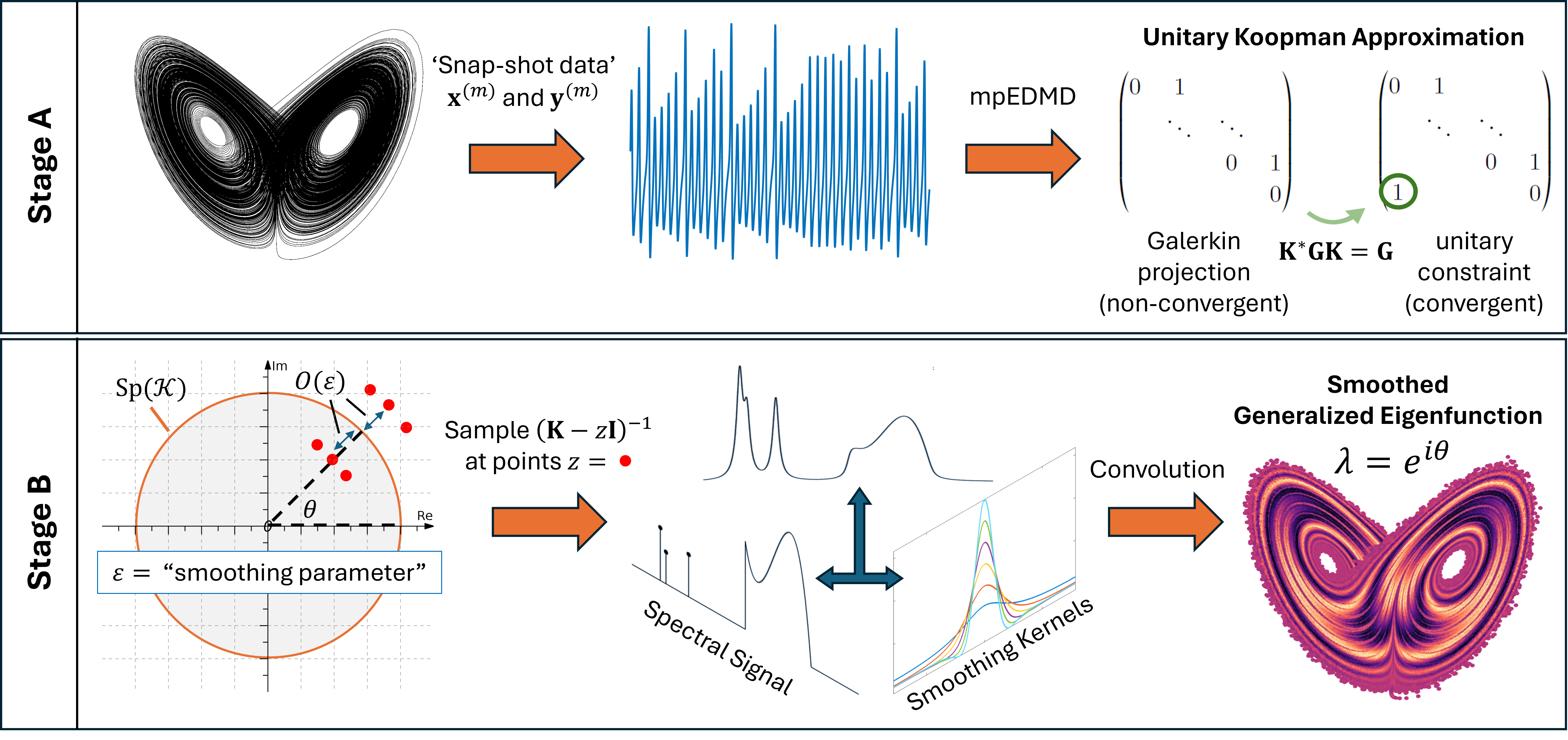
Figure 1: Schematic of Rigged DMD. Stage A consists of a data-driven unitary approximation of $\mathcal{K}$. Stage B consists of sampling the resolvent of this approximation to form a smoothed generalized Koopman eigenfunction (and Koopman modes) in the form of a wave-packet approximation. These generalized eigenfunctions provide a decomposition, even in the presence of continuous spectra. The full algorithm is given in Algorithm 1.

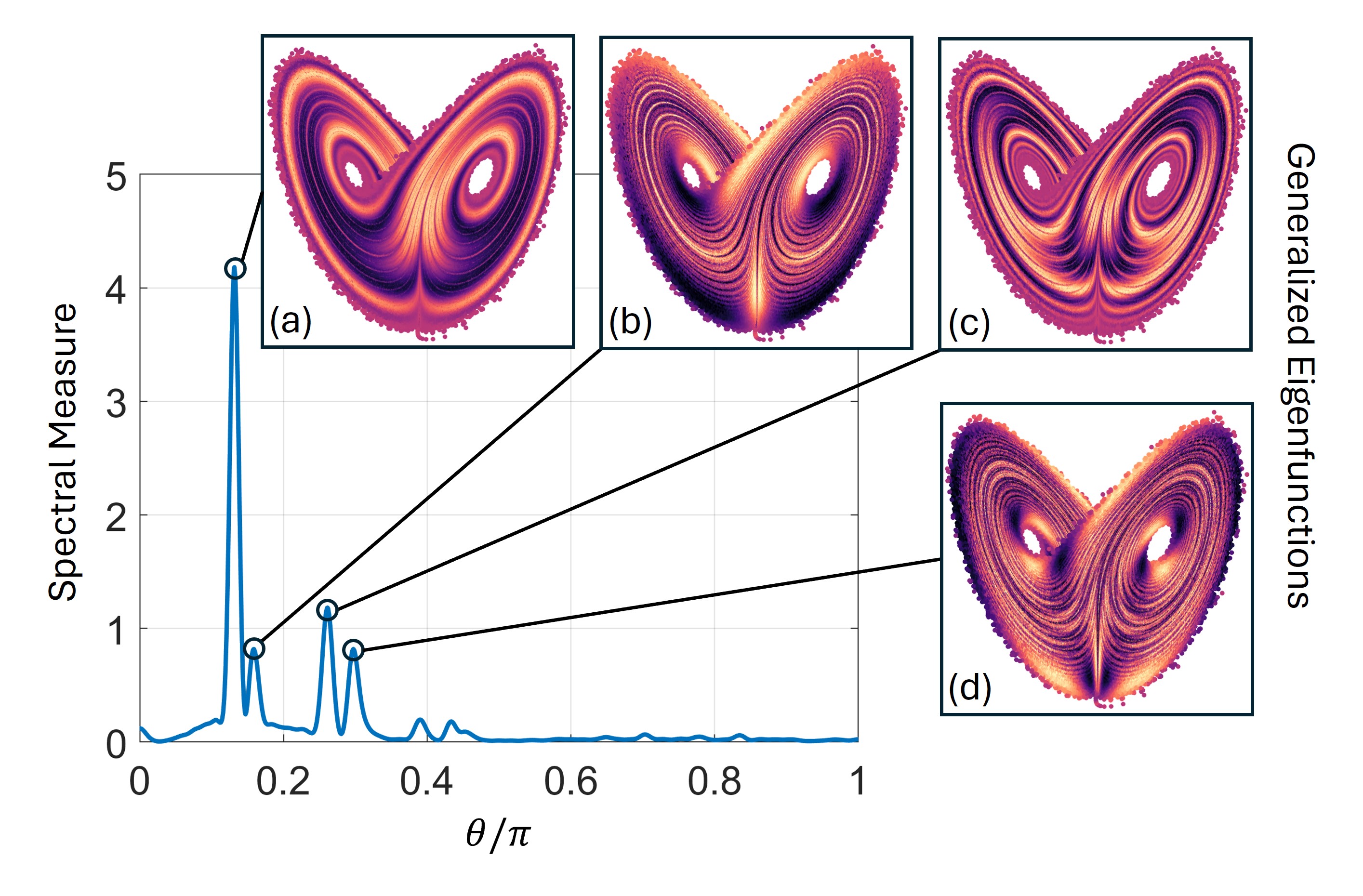
Figure 2: Spectral measure and generalized eigenfunctions for the Lorenz system computed using Rigged DMD. The spectral measure is continuous, and the generalized eigenfunctions are coherent.

This paper introduces a new Koopman mode decomposition and computational framework for unitary Koopman operators on a rigged Hilbert space (see Section 2.4). In the rigged Hilbert space, the discrete and continuous spectrum are treated on equal footing, and (almost) every point in the spectrum is associated with a set of coherent generalized eigenfunctions. Generalized eigenfunctions associated with the continuous spectrum are not elements of the Hilbert space. Instead, as distributions in the rigged Hilbert space, they represent coherent linear features of the observables that may be used to identify coherent patterns in Eq. 1.

Our algorithm, which we call Rigged DMD, computes smooth wave-packet approximations to generalized Koopman eigenfunctions using a two-stage framework (see Fig. 1). In the first stage, we use mpEDMD to construct a finite-dimensional unitary approximation to the Koopman operator from the snapshot data in Eq. 2. In the second stage, we use the mpEDMD resolvent to construct wave packets of observables with highly localized spectral content. These approximations converge to generalized eigenfunctions associated with both the discrete and the continuous spectrum (see Section 5). They are approximately coherent (see Theorem 5.13), achieve high orders of accuracy under natural regularity conditions on the spectral measure of $\mathcal{K}$ (see Theorem 5.9), and converge pointwise in regions where generalized eigenfunctions can be identified with smooth functions (see Theorem 5.11). For example, Figure 2 shows four wave-packet approximations to generalized eigenfunctions associated with the continuous spectrum of a Koopman operator on the Lorenz attractor.

There is extensive literature on rigged Hilbert spaces for self-adjoint operators in PDE analysis and quantum mechanics [40, 14, 49, 13, 12]. However, standard rigging techniques do not always apply to Koopman operators (consider the task of constructing a nuclear space on the Lorenz attractor). For this reason, we provide a novel method to construct nuclear spaces for unitary operators with sparse, infinite-dimensional matrix representations (see Section 6). This technique can be applied to any Koopman operator via time-delay embedding, enabling the computation of generalized Koopman eigenfunctions for the Lorenz attractor.

The paper is organized as follows. We review the spectral theory of unitary Koopman operators on Hilbert spaces and derive Koopman mode decompositions in a rigged Hilbert space in Section 2. The Rigged DMD algorithm is introduced in Section 3, and connections with previous work are discussed in Section 3.1. Data-driven approximations of the Koopman resolvent are discussed in Section 4, and wave-packet approximations are analyzed in Section 5. In Section 6, we develop a methodology to rig Hilbert spaces for Koopman operators. A variety of worked examples in Section 7 include: systems with a Lebesgue spectrum, illustrated by Arnold’s cat map; integrable systems, illustrated by the nonlinear pendulum; the Lorenz system, demonstrating the utility of the rigged Hilbert space construction via time-delay embedding; and a high-dimensional fluid flow scenario. General purpose code and all the examples of this paper can be found at: https://github.com/MColbrook/Rigged-Dynamic-Mode-Decomposition.

2 Background: Koopman mode decompositions

We assume that the system in Eq. 1 preserves a Borel measure $\omega$ (not necessarily finite), i.e., for measurable sets $S\subset\Omega$,

$$\omega(S)=\omega(\mathbf{F}^{-1}(S)),\quad\text{where}\quad\mathbf{F}^{-1}(S)=\{\mathbf{x}:\mathbf{F}(\mathbf{x})\in S\}.$$

Such systems preserve an energy or volume associated with $\omega$ and are ubiquitous [7, 34, 74, 46, 86]. Many systems admit invariant measures [55] or measure-preserving post-transient behavior [61]. We also assume that the dynamical system is invertible modulo $\omega$-null sets (see [35, Chapter 7]), so that $\mathcal{K}$ is a unitary operator on the Hilbert space $L^{2}(\Omega,\omega)$:

$$\mathcal{K}:L^{2}(\Omega,\omega)\rightarrow L^{2}(\Omega,\omega),\qquad\text{and}\qquad\mathcal{K}\mathcal{K}^{*}=\mathcal{K}^{*}\mathcal{K}=I.$$

Here, $\mathcal{K}^{*}$ denotes the adjoint of $\mathcal{K}$, and $I$ denotes the identity operator. The spectral theory of unitary operators provides a firm foundation for Koopman mode decompositions.

2.1 Eigenvalues and eigenfunctions

Suppose first that an observable $\phi\in L^{2}(\Omega,\omega)$ is an eigenfunction of $\mathcal{K}$ with eigenvalue $\lambda$. Then $\phi$ is a coherent observable, because

(4) $$\phi(\mathbf{x}_{n})=[\mathcal{K}^{n}\phi](\mathbf{x}_{0})=\lambda^{n}\phi(\mathbf{x}_{0})\qquad\text{for}\qquad n=0,1,2,\ldots.$$

The oscillation and decay/growth of the observable $\phi$ are dictated by the complex argument and absolute value of the eigenvalue $\lambda$, respectively. Eigenpairs $(\phi,\lambda)$ encode key information about coherent structures observed in the dynamics in Eq. 1. For example, the level sets of eigenfunctions determine invariant manifolds [63] and isostables [60] of the dynamical system.

If $\mathcal{K}$ has an invariant subspace spanned by eigenfunctions $\{\phi_{n}\}_{n=1}^{\infty}$, the Koopman mode decomposition (KMD) expands observables $\mathbf{g}=[g_{1},\ldots,g_{l}]^{T}$ in this subspace [61, 69]:

(5) $$\mathbf{g}(\mathbf{x})=\sum_{n=1}^{\infty}\mathbf{c}_{n}\phi_{n}(\mathbf{x}),\qquad\text{so that}\qquad\mathbf{g}(\mathbf{x}_{k})=\sum_{n=1}^{\infty}\mathbf{c}_{n}\lambda_{n}^{k}\phi_{n}(\mathbf{x}_{0}).$$

Here, $\lambda_{n}$ is the eigenvalue of $\mathcal{K}$ satisfying $\mathcal{K}\phi_{n}=\lambda_{n}\phi_{n}$, for $n=1,2,3,\ldots,$ and the expansion coefficients $\mathbf{c}_{n}$ are called the Koopman modes of $\mathbf{g}(\mathbf{x})$ [69]. The KMD provides key insights into the dynamical system, and truncated series may be used for reduced-order models [70, 66].

2.2 Spectrum and pseudoeigenfunctions

$\mathcal{K}$ may not have non-trivial eigenpairs, e.g., in Fig. 2. Instead, the correct generalization of the set of eigenvalues of $\mathcal{K}$ is the spectrum

$$\mathrm{Sp}(\mathcal{K})=\left\{z\in\mathbb{C}:(\mathcal{K}-zI)^{-1}\text{ does not exist as a bounded operator}\right\}\subset\mathbb{C}.$$

Since $\mathcal{K}$ is unitary, we have $\mathrm{Sp}(\mathcal{K})\subset\mathbb{T}=\{z\in\mathbb{C}:|z|=1\}$. The spectrum includes the set of eigenvalues of $\mathcal{K}$, but in general, it may contain points that are not eigenvalues and hence do not have an associated eigenfunction. However, there are approximately coherent observables associated with each point because $\mathcal{K}$ is unitary (therefore, normal). For each point $\lambda\in\mathrm{Sp}(\mathcal{K})$ and any $\delta>0$, there exists a $\phi_{\delta}\in L^{2}(\Omega,\omega)$ with norm one such that $\|(\mathcal{K}-\lambda I)\phi_{\delta}\|\leq\delta$. The observable $\phi_{\delta}$ is called a $\delta$-pseudoeigenfunction [81, p. 31] and satisfies

(6) $$\|\mathcal{K}^{n}\phi_{\delta}-\lambda^{n}\phi_{\delta}\|=\mathcal{O}(n\delta)\quad\forall n\in\mathbb{N}.$$

Like their eigenfunction counterparts, pseudoeigenfunctions encode significant information about the underlying dynamical system [65], such as the global stability of equilibria [59] and ergodic partitions [17]. However, they do not diagonalise the Koopman operator.

2.3 Spectral measures and diagonalization

The spectral theorem [29, Thm. X.4.11] provides a diagonalization of $\mathcal{K}$ using a projection-valued measure $\mathcal{E}$ supported on $\mathrm{Sp}(\mathcal{K})\subset\mathbb{T}$. To each Borel subset $S\subset\mathbb{T}$, $\mathcal{E}$ associates an orthogonal projection $\mathcal{E}(S)$, which one should think of as the spectral content of $\mathcal{K}$ on $S$. In particular, we have the following decompositions:

(7) $$g=\left(\int_{\mathbb{T}}1{\,\mathrm{d}}\mathcal{E}(\lambda)\right)g\qquad\text{and}\qquad\mathcal{K}g=\left(\int_{\mathbb{T}}\lambda\ \mathrm{d}\mathcal{E}(\lambda)\right)g\quad\forall g\in L^{2}(\Omega,\omega).$$

Moreover, the analogue of Eq. 4 is provided by a functional calculus on ${\rm Sp}(\mathcal{K})$, so that

$$g(\mathbf{x}_{n})=[\mathcal{K}^{n}g](\mathbf{x}_{0})=\left[\left(\int_{\mathbb{T}}\lambda^{n}\ \mathrm{d}\mathcal{E}(\lambda)\right)g\right](\mathbf{x}_{0})\quad\forall g\in L^{2}(\Omega,\omega).$$

While $\mathcal{E}$ associates invariant subspaces of $\mathcal{K}$ to measurable subsets of its spectrum, $\mathcal{E}$ is unable to associate coherent modes in $\mathcal{L}^{2}(\Omega,\omega)$ to points in the continuous spectrum.

The scalar-valued spectral measure of $\mathcal{K}$ with respect to $g\in L^{2}(\Omega,\omega)$ with $\|g\|=1$ is a probability measure supported on $\mathbb{T}$ and defined as $\mu_{g}(S)=\langle\mathcal{E}(S)g,g\rangle$. Following a change of variables $\lambda=\exp(i\theta)$, we consider the measures $\xi_{g}$ on the periodic interval ${[{-}\pi,\pi]_{\mathrm{per}}}$ so that $\xi_{g}(S)=\mu_{g}(\exp(iS))$ for $S\subset{[{-}\pi,\pi]_{\mathrm{per}}}$. Similarly, we make use of complex Borel measures $\xi_{g,f}(S)=\langle\mathcal{E}(\exp(iS))g,f\rangle$, for $f,g\in L^{2}(\Omega,\omega)$. The Lebesgue decompositions of the scalar spectral measures $\xi_{g}$ lead to a partition of the Hilbert space $L^{2}(\Omega,\omega)$ into closed subspaces $\mathcal{H}_{\mathrm{pp}}$ and $\mathcal{H}_{\mathrm{c}}$. Dynamics in $\mathcal{H}_{\mathrm{pp}}$ can be resolved via a discrete KMD in Eq. 5, whereas those in $\mathcal{H}_{\mathrm{c}}$ cannot. These subspaces find interpretations across various applications, including fluid mechanics [62], anomalous transport [90], and trajectory invariants/exponents [48].

2.4 Generalized eigenfunctions

To construct a KMD from coherent features, we replace the projection-valued measure with a generalized eigenfunction expansion. Generalized eigenfunctions are distributions on a subspace $\mathcal{S}\subset L^{2}(\Omega,\omega)$ of test functions, where $\mathcal{K}\mathcal{S}\subset\mathcal{S}$ and $\mathcal{S}$ admits a dense, continuous embedding into $L^{2}(\Omega,\omega)$ as a complete topological vector space. In this case, the dual of $L^{2}(\Omega,\omega)$ embeds densely and continuously into the space $\mathcal{S}^{*}$ of continuous linear functionals on $\mathcal{S}$. By identifying $L^{2}(\Omega,\omega)$ with its dual, one obtains a triple of dense, continuous embeddings $\mathcal{S}\subset L^{2}(\Omega,\omega)\subset\mathcal{S}^{*}$, referred to as a rigged Hilbert space. Since the inner product $\langle\cdot,\cdot\rangle$ on $L^{2}(\Omega,\omega)$ is conjugate linear in its second argument, the duality pairing $\langle\psi|\phi\rangle$ for $\psi\in\mathcal{S}^{*}$ and $\phi\in\mathcal{S}$ is equal to $\langle\phi,\overline{\psi}\rangle$ when both $\psi$ and $\phi$ are in $L^{2}(\Omega,\omega)$. Given $\psi\in\mathcal{S}^{*}$, it is useful to define its conjugate $\psi^{*}\in\mathcal{S}^{*}$ by $\langle\psi^{*}|\phi\rangle=\overline{\langle\psi|\overline{\phi}\rangle}$ for $\phi\in\mathcal{S}$. The Koopman operator has a continuous extension to $\mathcal{S}^{*}$ as $\smash{\langle\mathcal{K}\psi|\phi\rangle=\langle\psi|\overline{\mathcal{K}^{*}\overline{\phi}}\rangle=\langle\psi|\mathcal{K}^{*}\phi\rangle}$, where the second equality holds because $\mathcal{K}$ is a composition operator.

A functional $\psi\in\mathcal{S}^{*}$ is called a generalized eigenfunction of $\mathcal{K}$ if there is a $\lambda\in\mathbb{C}$ such that

(8) $$\smash{\langle\mathcal{K}\psi|\phi\rangle=\lambda\langle\psi|\phi\rangle\qquad\forall\phi\in\mathcal{S}}.$$

By the density of $\mathcal{S}$ in $\smash{L^{2}(\Omega,\omega)}$, $\smash{u\in L^{2}(\Omega,\omega)}$ is a generalized eigenfunction if and only if it is an eigenfunction. From Eq. 8, generalized eigenfunctions are coherent because

(9) $$\langle\mathcal{K}\psi|\phi\rangle=\lambda^{n}\langle\psi|\phi\rangle\qquad\text{for all}\qquad\phi\in\mathcal{S}\text{ and }n\in\mathbb{Z}.$$

To achieve a modal decomposition using generalized eigenfunctions, we require that $\mathcal{S}$ also be a countably Hilbert nuclear space [41, Ch. 1.3]. Then, there is a complete set of generalized eigenfunctions $\{g_{\theta,k}:\theta\in{[{-}\pi,\pi]_{\mathrm{per}}},k\in\mathcal{I}\}\subset\mathcal{S}^{*}$ such that for any $g\in\mathcal{S}$, it holds in $L^{2}(\Omega,\omega)$:

(10) $$g=\sum_{k\in\mathcal{I}}\int_{[{-}\pi,\pi]_{\mathrm{per}}}\!\!\!\!\!\langle g_{\varphi,k}^{*}|g\rangle g_{\varphi,k}{\,\mathrm{d}}\xi_{g_{k}}(\varphi),\quad\mathcal{K}g=\sum_{k\in\mathcal{I}}\int_{[{-}\pi,\pi]_{\mathrm{per}}}\!\!\!\!\!\exp(i\varphi)\langle g_{\varphi,k}^{*}|g\rangle g_{\varphi,k}{\,\mathrm{d}}\xi_{g_{k}}(\varphi).$$

The spectral measures $\{\xi_{g_{k}}\}$ reflect a choice of normalization and the multiplicity of $\lambda=\exp(i\theta)\in{\rm Sp}(\mathcal{K})$ is the number of nonzero functionals $\{g_{\theta,k}\}$. This expansion replaces the projection-valued measure expansion in Eq. 7 with a KMD, where the Koopman mode associated with $g_{\varphi,k}$ is the dual product $\langle g_{\varphi,k}^{*}|g\rangle$. For example, if each observable in $\mathbf{g}=[g_{1},\ldots,g_{l}]^{T}$ lies in $\mathcal{S}$, we recover the vectorized form of Eq. 10 as an analogue of the classic KMD in Eq. 5:

$$\mathbf{g}=\sum_{k\in\mathcal{I}}\int_{[{-}\pi,\pi]_{\mathrm{per}}}\!\!\!\!\!\langle g_{\varphi,k}^{*}|\mathbf{g}\rangle g_{\varphi,k}{\,\mathrm{d}}\xi_{g_{k}}(\varphi),\quad\text{so that}\quad\mathbf{g}=\sum_{k\in\mathcal{I}}\int_{[{-}\pi,\pi]_{\mathrm{per}}}\!\!\!\!\!\exp(in\varphi)\langle g_{\varphi,k}^{*}|\mathbf{g}\rangle g_{\varphi,k}{\,\mathrm{d}}\xi_{g_{k}}(\varphi).$$

Here, $\langle g_{\varphi,k}^{*}|\mathbf{g}\rangle$ is the Koopman mode associated with the point $\lambda=\exp(in\varphi)\in{\rm Sp}(\mathcal{K})$.

3 The Rigged DMD algorithm

To approximate generalized Koopman modes and eigenfunctions from the snaphot data in Eq. 2, we consider “wave-packet” observables of the form

(11) $$g_{\theta}^{\epsilon}=\sum_{k\in\mathcal{I}}\int_{[{-}\pi,\pi]_{\mathrm{per}}}\!\!\!\!\!K_{\epsilon}(\theta-\varphi)\,\langle g_{\varphi,k}^{*}|g\rangle g_{\varphi,k}{\,\mathrm{d}}\xi_{g_{k}}(\varphi)\in L^{2}(\Omega,\omega),\qquad\text{where}\qquad g\in\mathcal{S}.$$

This wave-packet approximates the part of Eq. 10 with spectral parameter $\lambda=\exp(i\theta)$ via convolution with $K_{\epsilon}$. The function $K_{\epsilon}$ is a highly localized smoothing kernel approximating a Dirac delta measure as $\epsilon\downarrow 0$. Therefore, the kernel filters out the contribution of unwanted modes to $g_{\theta}^{\epsilon}$ and amplifies the contribution of the desired modes at $\lambda=\exp(i\theta)$ for small $\epsilon$. In the limit as $\epsilon\downarrow 0$, we aim for $g_{\theta}^{\epsilon}$ to converge in a suitable sense (e.g., in $\mathcal{S}^{*}$) to a generalized eigenfunction of $\mathcal{K}$ associated with the point $\lambda=\exp(i\theta)$.

To compute $\smash{g_{\theta}^{\epsilon}}$, we exploit a connection between rational convolution kernels and the resolvent, $\smash{(\mathcal{K}-zI)^{-1}}$, of the Koopman operator. For example, let

(12) $$K^{\rm(P)}_{\epsilon}(\varphi)=\frac{1}{2\pi}\frac{(1+\epsilon)^{2}-1}{1+(1+\epsilon)^{2}-2(1+\epsilon)\cos(\varphi)}$$

be the Poisson kernel for the unit disc [50, p.16]. If we set $r=1+\epsilon$, then (see Section 5)

(13) $$g_{\theta}^{\epsilon}=\frac{1}{4\pi}\left[(\mathcal{K}+r^{-1}e^{i\theta}I)(\mathcal{K}-r^{-1}e^{i\theta}I)^{-1}-(\mathcal{K}+re^{i\theta}I)(\mathcal{K}-re^{i\theta}I)^{-1}\right]g.$$

Therefore, we can explicitly compute $g_{\theta}^{\epsilon}$ by sampling the resolvent at a few strategic points in the complex plane. Although the Poisson kernel produces low-order accurate approximations to the generalized eigenfunctions in general, we construct high-order accurate rational convolution kernels in Section 5.1 and analyze their convergence properties in Section 5.2.

The question remains: How can we approximate $\smash{(\mathcal{K}-zI)^{-1}}$ from the snapshot data in Eq. 2? A first attempt may project $\mathcal{K}$ onto a finite-dimensional subspace of observables. This is equivalent to using Extended Dynamic Mode Decomposition (EDMD) [87] in the large data limit $M\rightarrow\infty$, which generally does not work.

Example 3.1 (Non-convergence of EDMD).

Consider the Hilbert space $l^{2}(\mathbb{Z})$ with orthonormal basis $\{e_{j}\}_{j=-\infty}^{\infty}$. Let $\mathcal{K}$ be the bilateral shift defined by $\mathcal{K}e_{j}=e_{j-1}.$ This operator is unitary and ${\mathrm{Sp}}(\mathcal{K})=\mathbb{T}$. Such shifts commonly appear when considering the restriction of Koopman operators to subspaces of observables, and we will revisit this example in Section 7.2. If we restrict the operator to $\mathrm{span}\{e_{-N},\ldots,e_{N}\}$, the large data limit $M\rightarrow\infty$ of the EDMD matrix approximation of $\mathcal{K}$ is the finite $(2N+1)\times(2N+1)$ Jordan matrix

$$\mathbb{K}_{\text{EDMD}}=\begin{pmatrix}0&1&&\\ &\ddots&\ddots&\\ &&0&1\\ &&&0\\ \end{pmatrix},\quad\text{with}\quad(\mathbb{K}_{\text{EDMD}}-z\mathbf{I})^{-1}=\begin{pmatrix}\frac{-1}{z}&\frac{-1}{z^{2}}&\ldots&\frac{-1}{z^{k}}\\ &\ddots&\ddots&\vdots\\ &&\frac{-1}{z}&\frac{-1}{z^{2}}\\ &&&\frac{-1}{z}\\ \end{pmatrix}$$

The spectrum of $\mathbb{K}_{\text{EDMD}}$ is $\{0\}$ and severely unstable. For example, if $0<|z|<1$, then $(\mathbb{K}_{\text{EDMD}}-z\mathbf{I})^{-1}e_{0}=\sum_{j=1}^{N}-z^{-j}e_{-j}$ grows exponentially as $N\rightarrow\infty$, whereas $(\mathcal{K}-zI)^{-1}e_{0}=\sum_{j=1}^{\infty}z^{j-1}e_{j}.$ $\blacksquare$

To rectify this, we use mpEDMD, which computes the unitary part of a Galerkin projection of $\mathcal{K}$ onto a finite-dimensional subspace spanned by a dictionary $\{\psi_{1},\ldots,\psi_{N}\}\subset L^{2}(\Omega,\omega)$. This projection is computed using the snapshot data to approximate integration with respect to $\omega$. Utilizing the unitary part is crucial for achieving convergence (see Theorem 4.1). In Example 3.1, mpEDMD replaces the Jordan matrix with a circulant matrix

$$\begin{pmatrix}0&1&&\\ &\ddots&\ddots&\\ &&0&1\\ 1&&&0\\ \end{pmatrix},$$

effectively placing a $1$ in the bottom-left corner. In general, mpEDMD achieves a unitary approximation by taking the unitary part of a polar decomposition.

Algorithm 1 summarizes Rigged DMD, which can be split into two key stages (Fig. 1):

• Stage A: Use mpEDMD to compute a discretization of $\mathcal{K}$ and $g$, as detailed in Section 4. Step 2 represents the observable $g$ in terms of the mpEDMD eigenvectors, which are orthogonal with respect to a data-driven approximation of $\omega$.

• Stage B: Build wave-packet approximations through sampling the resolvent, as detailed in Section 5. Step 3 solves a small linear system to construct high-order rational smoothing kernels. Step 4 builds the wave-packet approximation. Step 5 computes spectral measures through an inner product.

Input: Snapshots $\{\mathbf{x}^{(m)},\mathbf{y}^{(m)}\}_{m=1}^{M}$, quadrature weights $\{w_{m}\}_{m=1}^{M}$, dictionary of observables $\{\psi_{j}\}_{j=1}^{N}$, $\{a_{j}\}_{j=1}^{m}$ with ${\rm Im}(a_{j})>0$, smoothing parameter $\epsilon>0$, $\Theta\subset{[{-}\pi,\pi]_{\mathrm{per}}}$, observable $g$.

Output: Vectors $\{\mathbf{g}_{\theta}:\theta\in\Theta\}$ such that each $\mathbf{\Psi}\mathbf{g}_{\theta}\in L^{2}(\Omega,\omega)$ is a wave-packet approximation to a generalized eigenfunction of $\mathcal{K}$ corresponding to spectral parameter $\lambda=\exp(i\theta)$. If desired, smoothed spectral measures $\{\xi(\theta):\theta\in\Theta\}$.

Algorithm 1 The Rigged DMD algorithm for computing generalized eigenfunctions of $\mathcal{K}$.

A few practical points are worth discussing:

• We work in mpEDMD eigenvector coordinates. Step 4 requires no matrix multiplication, and it is very cheap to compute wave-packet approximations for different $\theta$.

• Wave-packets can be evaluated at any point $\mathbf{x}\in\Omega$ through the feature map $\mathbf{\Psi}(\mathbf{x})=[\psi_{1}(\mathbf{x})\cdots\psi_{{N}}(\mathbf{x})]$. For example, we can evaluate wave-packets at the snapshot data.

• Spectral measures are also cheap to evaluate at several $\theta$. We recommend choosing an equispaced $\theta$ grid for visualization, such as in Fig. 2.

• If the state space dimension $d$ is large, it may be difficult to visualize $g_{\theta}^{\epsilon}$. Instead, we can visualize the Koopman modes $\langle g_{\varphi,k}^{*}|\mathbf{g}\rangle$ for a collection of observables $\mathbf{g}=[g_{1},\ldots,g_{l}]^{T}$. This post-processing step is summarized in Algorithm 2 and can also be achieved via normalising by the smoothed spectral measures computed in Algorithm 1.

To explain how and why Rigged DMD works, we describe stages A and B and analyze key notions of convergence in greater detail in Section 4 and Section 5 below. The reader may safely skip to the examples in Section 7.

Input: Snapshot data $\{\mathbf{x}^{(m)},\mathbf{y}^{(m)}\}_{m=1}^{M}$, quadrature weights $\{w_{m}\}_{m=1}^{M}$, dictionary of observables $\{\psi_{j}\}_{j=1}^{N}$, $\{a_{j}\}_{j=1}^{m}$ with ${\rm Im}(a_{j})>0$, smoothing parameter $\epsilon>0$, angles $\Theta\subset{[{-}\pi,\pi]_{\mathrm{per}}}$, observables $\mathbf{g}=[g_{1},\ldots,g_{l}]^{T}$.

1:Apply steps 1 – 5 of Rigged DMD (Algorithm 1) for each observable $g_{p}$ to compute $\widetilde{\mathbf{g}}_{\theta}^{(p)}$ (where the superscript denotes dependence on $p$) for $p=1,\ldots,l$ and $\theta\in\Theta$.

2:For each $\theta\in\Theta$, compute the mean $\smash{\widetilde{\mathbf{g}}_{\theta}=\frac{1}{l}\sum_{p=1}^{l}\widetilde{\mathbf{g}}_{\theta}^{(p)}}$ and the vector $\mathbf{c}_{\theta}\in\mathbb{C}^{l}$ defined component-wise by $[\mathbf{c}_{\theta}]_{p}=\widetilde{\mathbf{g}}_{\theta}^{*}\widetilde{\mathbf{g}}_{\theta}^{(p)}.$

Output: Vectors $\{\mathbf{c}_{\theta}:\theta\in\Theta\}$.

Algorithm 2 Post-processing of Rigged DMD to compute generalized Koopman modes.

3.1 Connections with previous work

Generalized eigenfunctions of Perron–Frobenius operators, which are pre-adjoints of Koopman operators, are well-studied. The decay rates of correlation functions, known as Pollicott–Ruelle resonances [68, 71], correspond to a distinct type of generalized eigenvalue of the Perron–Frobenius operator. Numerous studies have explored these expansions for specific examples of maps [4, 44, 72, 37, 45, 38, 79, 2, 3, 33, 1, 77]. A key distinction between these works and ours is that Pollicott–Ruelle resonances typically do not lie on the unit circle, corresponding instead to extensions of Koopman operators via meromorphic extensions of the resolvent. Operators that admit such extensions are termed Fredholm–Riesz operators [10]. In contrast, our work achieves a generalized eigenfunction expansion with eigenvalues on the unit circle and makes no assumption beyond $\mathcal{K}$ being unitary. Recently, Bandtlow, Just, and Slipantschuk [75, 11] and Wormell [88] have found a significant link in certain systems: EDMD eigenvalues in the large subspace limit can correspond to these resonances. Meanwhile, generalized eigenfunctions associated with the Koopman operator side have been less explored, with Mezić’s work on integrable Hamiltonian systems with one degree of freedom [64] being a notable exception. We revisit this example in Section 7.2, providing an explicit expansion for any number of degrees of freedom. A general-purpose algorithm for computing generalized eigenfunctions of Koopman operators from snapshot data in Eq. 2 has yet to be developed. Rigged DMD addresses this gap.

Spectral measures are formed from one-dimensional projections of generalized eigenfunctions. Methods for computing spectral measures of Koopman operators have been developed in the last few years. We have already mentioned ResDMD [28] and mpEDMD [23]. ResDMD computes smoothed approximations of spectral measures associated with general measure-preserving dynamical systems using either the resolvent operator or filters applied to correlations. The paper [28] includes explicit high-order convergence theorems for the computation of spectral measures in various senses, including the density of the continuous spectrum, spectral projections of subsets of the unit circle, and the discrete spectrum. Similar smoothing techniques can also be used for self-adjoint operators [19]. The spectral measures of the mpEDMD approximations converge weakly to their infinite-dimensional counterparts. Other methods include compactification for Koopman generators of continuous-time systems [32, 85], the partitioning of state space to obtain periodic approximations [42, 43], post-processing of the moments of spectral measures of ergodic systems using the Christoffel–Darboux kernel [53], and harmonic averaging and Welch’s method for post-transient flows [6].

The above papers compute spectral measures as opposed to generalized eigenfunctions. Nevertheless, we build on some of the above techniques. We use mpEDMD as a discretization method to construct data-driven approximations of the resolvent $(\mathcal{K}-zI)^{-1}$. Example 3.1 demonstrates the necessity for using mpEDMD. We then use the resolvent to compute smoothed approximations of generalized eigenfunctions. This smoothing is analogous to ResDMD, which computed smoothed approximations of spectral measures.

4 Data-driven computation of the resolvent

To compute the resolvent $(\mathcal{K}-zI)^{-1}g$, we will apply mpEDMD [23], which enforces measure-preserving approximations of $\mathcal{K}$. The mpEDMD algorithm is simple and robust, with no tuning parameters. Importantly, one can show its convergence of spectral properties and the resolvent (see Section 4.3).

4.1 Extended DMD

The starting point of EDMD [87] is a dictionary $\{\psi_{1},\ldots,\psi_{N}\}\subset L^{2}(\Omega,\omega)$, i.e., a list of observables. These observables generate a finite-dimensional subspace $V_{N}=\mathrm{span}\{\psi_{1},\ldots,\psi_{N}\}$. Utilizing the snapshot data in Eq. 2, EDMD constructs a matrix $\mathbb{K}_{\text{EDMD}}\in\mathbb{C}^{N\times N}$. This matrix acts on coefficients within expansions in terms of the dictionary to approximate the action of the Koopman operator on $V_{N}$:

$${[\mathcal{K}\psi_{j}](\mathbf{x})=\psi_{j}(\mathbf{F}(\mathbf{x}))\approx\sum_{i=1}^{N}(\mathbb{K}_{\text{EDMD}})_{ij}\psi_{i}(\mathbf{x})},\quad 1\leq j\leq{N}.$$

To build $\mathbb{K}_{\text{EDMD}}$, we view the snapshot data $\{\mathbf{x}^{(m)}\}_{m=1}^{M}$ as quadrature nodes for integration with respect to $\omega$ and weights $\{w_{m}\}_{m=1}^{M}$. Define the vector-valued feature map $\mathbf{\Psi}(\mathbf{x})=\begin{bmatrix}\psi_{1}(\mathbf{x})&\cdots&\psi_{{N}}(\mathbf{x})\end{bmatrix}\in\mathbb{C}^{1\times{N}}$, the weight matrix $\mathbf{W}=\mathrm{diag}(w_{1},\ldots,w_{M})$, and let

(14) $$\begin{split}\mathbf{\Psi}_{X}=\begin{pmatrix}\mathbf{\Psi}(\mathbf{x}^{(1)})\\ \vdots\\ \mathbf{\Psi}(\mathbf{x}^{(M)})\end{pmatrix}\in\mathbb{C}^{M\times N},\quad\mathbf{\Psi}_{Y}=\begin{pmatrix}\mathbf{\Psi}(\mathbf{y}^{(1)})\\ \vdots\\ \mathbf{\Psi}(\mathbf{y}^{(M)})\end{pmatrix}\in\mathbb{C}^{M\times N}.\end{split}$$

Assuming that the quadrature approximations are convergent, we have that

(15) $$\lim_{M\rightarrow\infty}[\mathbf{\Psi}_{X}^{*}\mathbf{W}\mathbf{\Psi}_{X}]_{jk}=\langle\psi_{k},\psi_{j}\rangle\quad\text{ and }\quad\lim_{M\rightarrow\infty}[\mathbf{\Psi}_{X}^{*}\mathbf{W}\mathbf{\Psi}_{Y}]_{jk}=\langle\mathcal{K}\psi_{k},\psi_{j}\rangle.$$

Therefore, the EDMD matrix is defined as (without loss of generality, ${\rm rank}(\mathbf{W}^{1/2}\mathbf{\Psi}_{X})=N$)

$$\mathbb{K}_{\text{EDMD}}=(\mathbf{W}^{1/2}\mathbf{\Psi}_{X})^{\dagger}\mathbf{W}^{1/2}\mathbf{\Psi}_{Y}=(\mathbf{\Psi}_{X}^{*}\mathbf{W}\mathbf{\Psi}_{X})^{\dagger}\mathbf{\Psi}_{X}^{*}\mathbf{W}\mathbf{\Psi}_{Y},$$

where ‘$\dagger$’ denotes the pseudoinverse. Hence, $\mathbb{K}_{\text{EDMD}}$ approaches a matrix representation of $\mathcal{P}_{V_{N}}\mathcal{K}\mathcal{P}_{V_{N}}^{*}$ in the large data limit, where $\mathcal{P}_{V_{N}}$ denotes the orthogonal projection onto $V_{N}$.

4.2 Measure-preserving EDMD

The Gram matrix $\mathbf{G}=\mathbf{\Psi}_{X}^{*}\mathbf{W}\mathbf{\Psi}_{X}$ provides an approximation of the inner product $\langle\cdot,\cdot\rangle$ on $L^{2}(\Omega,\omega)$. Given $\mathbf{h},\mathbf{g}\in\mathbb{C}^{N}$, we have that

(16) $$\mathbf{h}^{*}\mathbf{G}\mathbf{g}=\sum_{j,k=1}^{N}\overline{\mathbf{h}_{j}}\mathbf{g}_{k}\mathbf{G}_{j,k}\approx\sum_{j,k=1}^{N}\overline{\mathbf{h}_{j}}\mathbf{g}_{k}\langle\psi_{k},\psi_{j}\rangle=\langle\mathbf{\Psi}\mathbf{g},\mathbf{\Psi}\mathbf{h}\rangle.$$

If the convergence in Eq. 15 holds, the left-hand side of Eq. 16 converges to the right-hand side as $M\rightarrow\infty$. Hence, if $g=\mathbf{\Psi}\mathbf{g}\in V_{N}$ and we approximate $\mathcal{K}$ on $V_{N}$ by a matrix $\mathbf{K}$,

$$\|g\|^{2}\approx\mathbf{g}^{*}\mathbf{G}\mathbf{g},\quad\|\mathcal{K}g\|^{2}\approx\|\mathbf{\Psi}\mathbf{K}\mathbf{g}\|^{2}\approx\mathbf{g}^{*}\mathbf{K}^{*}\mathbf{G}\mathbf{K}\mathbf{g}.$$

Since $\mathcal{K}$ is an isometry, $\|g\|^{2}=\|\mathcal{K}g\|^{2}.$ The mpEDMD algorithm combines EDMD with the constraint $\mathbf{K}^{*}\mathbf{G}\mathbf{K}=\mathbf{G}$. In a nutshell, we enforce that our Galerkin approximation is an isometry with respect to the learned, data-driven inner product induced by $\mathbf{G}$.

Algorithm 3 summarizes the computation of $\mathbf{K}$ and its eigendecomposition. Since $\mathbf{K}$ is similar to a unitary matrix, its eigenvalues lie along the unit circle. Note that mpEDMD can be used with generic dictionary choices.

Input: Snapshots $\{\mathbf{x}^{(m)},\mathbf{y}^{(m)}\}_{m=1}^{M}$, quadrature weights $\{w_{m}\}_{m=1}^{M}$, dictionary of observables $\{\psi_{j}\}_{j=1}^{N}$.

1:Compute the matrices $\mathbf{\Psi}_{X}$ and $\mathbf{\Psi}_{Y}$ defined in Eq. 14 and $\mathbf{W}=\mathrm{diag}(w_{1},\ldots,w_{M})$.

2:Compute an economy QR decomposition $\mathbf{W}^{1/2}\mathbf{\Psi}_{X}=\mathbf{Q}\mathbf{R}$, where $\mathbf{Q}\in\mathbb{C}^{M\times N},\mathbf{R}\in\mathbb{C}^{N\times N}$.

3:Compute an SVD of $(\mathbf{R}^{-1})^{*}\mathbf{\Psi}_{Y}^{*}\mathbf{W}^{1/2}\mathbf{Q}=\mathbf{U}_{1}\mathbf{\Sigma}\mathbf{U}_{2}^{*}$.

4:Compute the eigendecomposition $\mathbf{U}_{2}\mathbf{U}_{1}^{*}=\hat{\mathbf{V}}\mathbf{\Lambda}\hat{\mathbf{V}}^{*}$ (via a Schur decomposition).

5:Compute $\mathbf{K}=\mathbf{R}^{-1}\mathbf{U}_{2}\mathbf{U}_{1}^{*}\mathbf{R}$ and $\mathbf{V}=\mathbf{R}^{-1}\hat{\mathbf{V}}$.

Output: Koopman matrix $\mathbf{K}$, with eigenvectors $\mathbf{V}$ and eigenvalues $\mathbf{\Lambda}$.

Algorithm 3 The mpEDMD algorithm [23] using a QR decomposition (see [24]). For stability, we compute the eigendecomposition of $\mathbf{K}$ via the unitary matrix $\mathbf{U}_{2}\mathbf{U}_{1}^{*}$.

4.3 Convergence to the resolvent

The following theorem shows that mpEDMD provides convergent approximations of $(\mathcal{K}-zI)^{-1}$ for $z\not\in\mathbb{T}$. Combined with the results of Section 5.2, this theorem implies the convergence of Rigged DMD in the large data ($M\rightarrow\infty$) and large dictionary ($N\rightarrow\infty$) limits as $\epsilon\downarrow 0$. In practice, $\epsilon$ is chosen adaptively depending on $M$ and $N$ or vice versa.

Theorem 4.1.

Suppose that $\lim_{N\rightarrow\infty}\!\mathrm{dist}(h,V_{N})=0$ for all $h\in L^{2}(\Omega,\omega)$ and Eq. 15 holds. Then for any $z\in\mathbb{C}\backslash\mathbb{T}$, $g\in L^{2}(\Omega,\omega)$ and $\mathbf{g}_{N}\in\mathbb{C}^{N}$ with $\lim_{N\rightarrow\infty}\|g-\mathbf{\Psi}\mathbf{g}_{N}\|=0$,

(17) $$\lim_{N\rightarrow\infty}\limsup_{M\rightarrow\infty}\|(\mathcal{K}-zI)^{-1}g-\mathbf{\Psi}(\mathbf{K}-z\mathbf{I})^{-1}\mathbf{g}_{N}\|=0.$$

Proof 4.2.

See Appendix A.

As we saw in Example 3.1, the convergence in Eq. 17 need not hold for methods such as EDMD. In particular, convergence in the strong operator topology (the convergence of EDMD) need not imply convergence of the resolvent. The fact that mpEDMD provides a measure-preserving approximation is crucial to Theorem 4.1.

5 Smooth wave-packet approximations to generalized eigenfunctions

To recover generalized eigenfunctions of $\mathcal{K}$ from sampling the resolvent $\smash{(\mathcal{K}-zI)^{-1}}$, we link $\smash{(\mathcal{K}-zI)^{-1}}$ to generalized eigenfunction in two steps. First, generalized eigenfunctions diagonalize the spectral measure on the rigged Hilbert space. For each Borel subset $S\subset{[{-}\pi,\pi]_{\mathrm{per}}}$ [36],

(18) $$\mathcal{E}(S)g=\sum_{k\in\mathcal{I}}\int_{S}\langle g_{\varphi,k}^{*}|g\rangle g_{\varphi,k}{\,\mathrm{d}}\xi_{g_{k}}(\varphi)\qquad\text{for all}\qquad g\in\mathcal{S}.$$

Second, the action of the projection-valued spectral measure $\mathcal{E}$ on observables can be recovered from the resolvent via the Carathéodory function of $\mathcal{E}$, defined as

(19) $$F_{\mathcal{E}}(z)=\int_{{[{-}\pi,\pi]_{\mathrm{per}}}}\frac{e^{i\varphi}+z}{e^{i\varphi}-z}{\,\mathrm{d}}\mathcal{E}(\varphi)=(\mathcal{K}+zI)(\mathcal{K}-zI)^{-1},\quad|z|\neq 1.$$

The second equality follows from the functional calculus of $\mathcal{K}$. Writing $z=re^{i\theta}$ in modulus-argument form and assuming that $r=(1+\epsilon)>1$, one finds that (c.f. Eqs. 11, 12 and 13)

(20) $$\frac{1}{4\pi}\left[F_{\mathcal{E}}(r^{-1}e^{i\theta})-F_{\mathcal{E}}(re^{i\theta})\right]=\frac{1}{2\pi}\int_{{[{-}\pi,\pi]_{\mathrm{per}}}}\frac{(r^{2}-1){\,\mathrm{d}}\mathcal{E}(\varphi)}{1+r^{2}-2r\cos(\theta-\varphi)}=[K^{\rm(P)}_{\epsilon}*\mathcal{E}](\theta).$$

The right-hand side is a convolution of $\mathcal{E}$ with the Poisson kernel defined in Eq. 12. Figure 3 illustrates the geometry of the left-hand side in the complex spectral domain.

Stone’s classic formula [76] recovers $\mathcal{E}$ by taking $r=(1+\epsilon)\downarrow 1$. Similarly, we can combine Eq. 18 and Eq. 20 to recover the generalized Koopman modes and eigenfunctions from $F_{\mathcal{E}}(z)$. We obtain convergence rates for wave-packet approximations to Koopman modes in the continuous spectrum under mild regularity conditions on spectral measures of $\mathcal{K}$. We denote the interior of a closed interval $\mathcal{I}$ by ${\rm int}(\mathcal{I})$ and write $g\in\mathcal{C}^{n,\alpha}(\mathcal{I})$ for a function with $n\in\mathbb{N}\cup\{0\}$ continuous derivatives on $\mathcal{I}$ with an $\alpha$-Hölder continuous $n$th derivative.

Theorem 5.1.

Suppose that the spectrum of $\mathcal{K}$ is absolutely continuous on the closed interval $\mathcal{I}\subset{[{-}\pi,\pi]_{\mathrm{per}}}$. Given $g,\phi\in\mathcal{S}$, let $\rho_{g,\phi}$ be the Radon–Nikodym derivative of the absolutely continuous component of $\xi_{g,\phi}$, and suppose that $\rho_{g,\phi}\in\mathcal{C}^{n,\alpha}(\mathcal{I})$ with $n\in\mathbb{N}\cup\{0\}$ and $\alpha\in[0,1]$. Denoting $g_{\theta}^{\epsilon}=\smash{[K^{\rm(P)}_{\epsilon}*\mathcal{E}](\theta)g}$, for any fixed $\theta_{0}\in{\rm int}(\mathcal{I})$, it holds that

$$\left|\langle g_{\theta_{0}}^{\epsilon}|\overline{\phi}\rangle-\rho_{g}(\theta_{0})\langle u_{\theta_{0}}|\overline{\phi}\rangle\right|=\mathcal{O}(\epsilon\,{\log(1+\epsilon^{-1})})+\mathcal{O}(\epsilon^{\alpha})\qquad\text{as}\qquad\epsilon\downarrow 0.$$

Here, $u_{\theta}\in\mathcal{S}^{*}$ is a generalized eigenfunction of $\mathcal{K}$ satisfying Eq. 8 with $\lambda=\exp(i\theta)$. Moreover, in general, the convergence rate $\mathcal{O}(\epsilon\,{\log(1+\epsilon^{-1})})$ is optimal for the Poisson kernel.

Proof 5.2.

See Appendix C.

The factor of $\rho_{g}(\theta)$ in Theorem 5.1 is equivalent to a renormalization of the generalized eigenfunctions in Eq. 10 so that $\{g_{\theta}^{\epsilon}\}$ are orthonormal with respect to Lebesgue measure on the continuous spectrum of $\mathcal{K}$, rather than with respect to a spectral measure of $\mathcal{K}$, in the limit $\epsilon\downarrow 0$. If desired, $g_{\theta}^{\epsilon}$ can easily be rescaled with the smoothed measure computed in Algorithm 1.

         

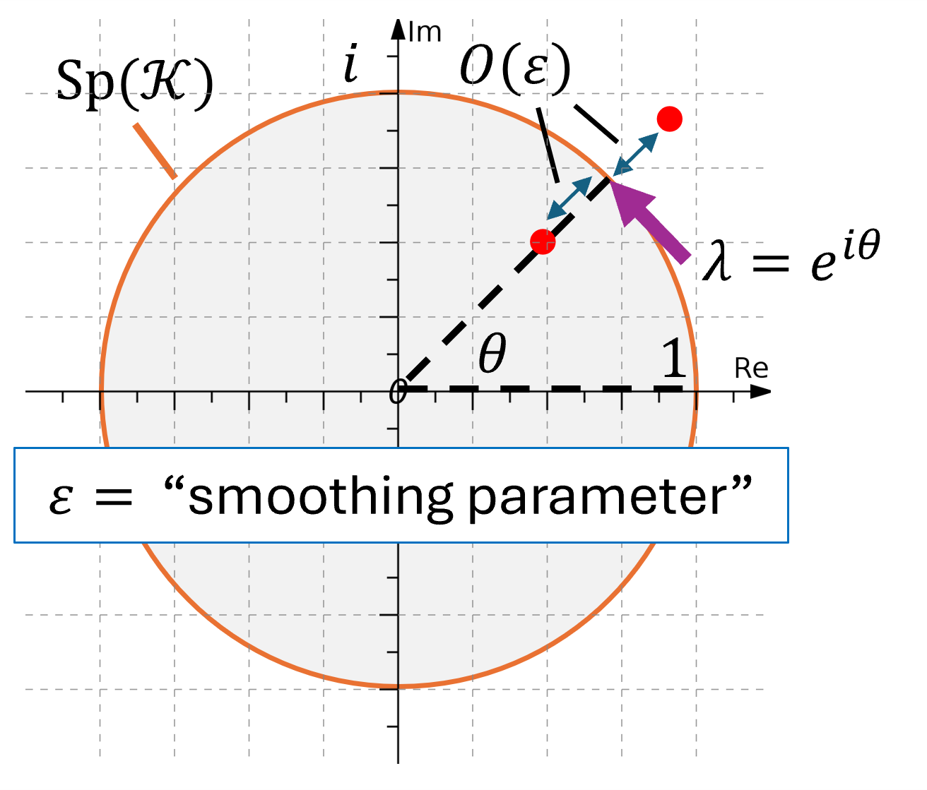
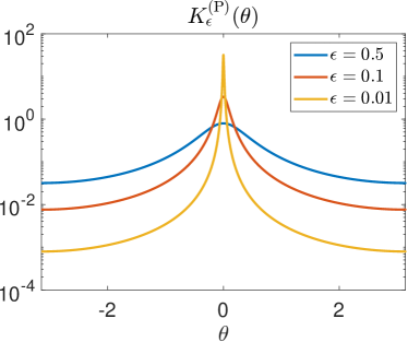
Figure 3: The essence of Stone’s formula. Left: The points $z$ marked with $\bullet$ are where we evaluate $(\mathcal{K}-zI)^{-1}$, at a distance $\epsilon$ and $1-1/(1+\epsilon)$ from the unit circle. Right: The Poisson kernel for the unit disc. As $\epsilon\downarrow 0$, the Poisson kernel converges in the sense of distributions to a Dirac delta distribution.

In practice, the sublinear convergence rates associated with the Poisson kernel present a computational bottleneck. As noted in [28, Figure 10], as $\epsilon\downarrow 0$, the computational cost typically increases because a larger dictionary of observables is required to compute the resolvent $(\mathcal{K}-zI)^{-1}$ and, consequently, a larger collection of snapshot data is required. Therefore, keeping $\epsilon$ from becoming too small is crucial.

5.1 High-order kernels

To alleviate the computational burden associated with slow convergence in the smoothing parameter $\epsilon$, we can replace the Poisson kernel with generalizations that achieve faster convergence rates as $\epsilon\downarrow 0$. Building on [28], we now use Carathéodory functions to develop a general, streamlined framework for high-order convolution kernels on the unit circle. Our starting point is defining an $m$th order periodic kernel.

Definition 5.3 ($m$th order periodic kernel).

Let $m\in\mathbb{N}$ and $\left\{K_{\epsilon}^{\mathbb{T}}:0<\epsilon\leq 1\right\}=\{K_{\epsilon}^{\mathbb{T}}\}$ be a family of continuous functions on the periodic interval ${[{-}\pi,\pi]_{\mathrm{per}}}$. We say that $\{K_{\epsilon}^{\mathbb{T}}\}$ is an $m$th order kernel for ${[{-}\pi,\pi]_{\mathrm{per}}}$ if it satisfies the following three properties:

• Normalized: $\int_{-\pi}^{\pi}K_{\epsilon}^{\mathbb{T}}(\theta){\,\mathrm{d}}\theta=1$.

• Approximately constant Fourier coefficients: There exists a constant $C_{K}$ such that for any integer $n=1,\ldots,m-1$,

  (21) $$\left|\int_{-\pi}^{\pi}K_{\epsilon}^{\mathbb{T}}(-\theta)e^{in\theta}{\,\mathrm{d}}\theta-1\right|\leq C_{K}\epsilon^{m}{\log(1+\epsilon^{-1})}.$$

• Concentration around zero: For any $\theta\in{[{-}\pi,\pi]_{\mathrm{per}}}$ and $0<\epsilon\leq 1$,

  (22) $$\left|K_{\epsilon}^{\mathbb{T}}(\theta)\right|\leq\frac{C_{K}\epsilon^{m}}{(\epsilon+|\theta|)^{m+1}}.$$

The name of this class of kernels is justified in Section 5.2, where we provide high-order convergence theorems. We consider continuous kernels since this implies that for any complex Borel measure $\xi$ on ${[{-}\pi,\pi]_{\mathrm{per}}}$, the function

$${[{-}\pi,\pi]_{\mathrm{per}}}\ni\varphi\mapsto\int_{{[{-}\pi,\pi]_{\mathrm{per}}}}K_{\epsilon}^{\mathbb{T}}(\varphi-\theta){\,\mathrm{d}}\xi(\theta)=\int_{{[{-}\pi,\pi]_{\mathrm{per}}}}K_{\epsilon}^{\mathbb{T}}(\theta){\,\mathrm{d}}\xi(\varphi-\theta)$$

is continuous. While the Poisson kernel for the unit disc in Eq. 12 is a first-order kernel, our goal is to build high-order kernels that can be expressed in terms of the Carathéodory function. We construct these from high-order rational kernels designed for the real line $\mathbb{R}$ [19].

Definition 5.4 ($m$th order kernel for $\mathbb{R}$).

Let $m\in\mathbb{N}$. We say that a continuous bounded function $K$ on $\mathbb{R}$ is an $m$th order kernel (for $\mathbb{R}$) if it satisfies the following three properties:

• Normalized: $K$ is integrable and $\int_{\mathbb{R}}K(x){\,\mathrm{d}}x=1$.

• Zero moments: $K(x)x^{j}$ is integrable and $\int_{\mathbb{R}}K(x)x^{j}{\,\mathrm{d}}x=0$ for $j=1,\ldots,m-1$.

• Decay at $\pm\infty$: There is a constant $C_{K}$, independent of $x$, such that

  (23) $$\left|K(x)\right|\leq\frac{C_{K}}{(1+\left|x\right|)^{m+1}}\quad\forall x\in\mathbb{R}.$$

The connection between Definition 5.3 and Definition 5.4 is the following proposition.

Proposition 5.5 (Periodic summation of kernels).

Let $K$ be an $m$th order kernel for $\mathbb{R}$ and

$$K_{\epsilon}^{\mathbb{T}}(\theta)=\sum_{n\in\mathbb{Z}}K_{\epsilon}(\theta+2\pi n)=\frac{1}{\epsilon}\sum_{n\in\mathbb{Z}}K\left(\frac{\theta+2\pi n}{\epsilon}\right),\quad 0<\epsilon\leq 1,$$

be its periodic summation. Then $\{K_{\epsilon}^{\mathbb{T}}\}$ is an $m$th order kernel for ${[{-}\pi,\pi]_{\mathrm{per}}}$.

Proof 5.6.

See Appendix B.

Suppose now that $K$ is an $m$th order kernel for $\mathbb{R}$ of the form

(24) $$K(x)=\frac{1}{2\pi i}\sum_{j=1}^{m}\left(\frac{\alpha_{j}}{x-a_{j}}-\frac{\beta_{j}}{x-b_{j}}\right),$$

where $a_{1},\ldots,a_{m}$ are any distinct points in the upper half-plane and $b_{1},\ldots,b_{m}$ are any distinct points in the lower half-plane. In [19], it is shown that $K$ is an $m$th order kernel for $\mathbb{R}$ if

(25) $$\begin{pmatrix}1&\dots&1\\ a_{1}&\dots&a_{m}\\ \vdots&\ddots&\vdots\\ a_{1}^{m-1}&\dots&a_{m}^{m-1}\end{pmatrix}\begin{pmatrix}\alpha_{1}\\ \alpha_{2}\\ \vdots\\ \alpha_{m}\end{pmatrix}\!=\begin{pmatrix}1&\dots&1\\ b_{1}&\dots&b_{m}\\ \vdots&\ddots&\vdots\\ b_{1}^{m-1}&\dots&b_{m}^{m-1}\end{pmatrix}\begin{pmatrix}\beta_{1}\\ \beta_{2}\\ \vdots\\ \beta_{m}\end{pmatrix}=\begin{pmatrix}1\\ 0\\ \vdots\\ 0\end{pmatrix}.$$

The following proposition expresses the periodic summation of these kernels in terms of the Carathéodory function. This result provides the basis for stage B in Algorithm 1.

Proposition 5.7.

Let $\{K_{\epsilon}^{\mathbb{T}}\}$ be the periodic summation (Proposition 5.5) of the $m$th order kernel for $\mathbb{R}$ in Eq. 24, where the residues $\{\alpha_{j},\beta_{j}\}$ satisfy Eq. 25. Then

(26) $$\left[K_{\epsilon}^{\mathbb{T}}\ast\mathcal{E}\right](\theta)=\frac{-1}{4\pi}\sum_{j=1}^{m}\left(\alpha_{j}F_{\mathcal{E}}(e^{i\theta-i\epsilon a_{j}})-\beta_{j}F_{\mathcal{E}}(e^{i\theta-i\epsilon b_{j}})\right).$$

Moreover, if $b_{j}=\overline{a_{j}}$ and $\beta_{j}=\overline{\alpha_{j}}$, then

$$\left[K_{\epsilon}^{\mathbb{T}}\ast\xi_{g}\right](\theta_{0}) =\frac{-1}{2\pi}\sum_{j=1}^{m}{\rm Re}\left(\alpha_{j}\left\langle(\mathcal{K}-e^{i\theta-i\epsilon a_{j}}I)^{-1}g,(\mathcal{K}+e^{i\theta-i\epsilon a_{j}}I)^{*}g\right\rangle\right).$$

Proof 5.8.

See Appendix B.

For computations, we use equally spaced poles in $[-1,1]$ with

(27) $$a_{j}=\frac{2j}{m+1}-1+i,\quad b_{j}=\overline{a_{j}},\quad 1\leq j\leq m.$$

We determine $\alpha_{j}=\overline{\beta_{j}}$ by solving Eq. 25. Fig. 4 shows these kernels for $m=1,\ldots,6$.

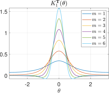
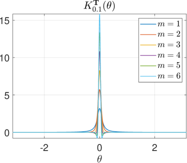
Figure 4: The $m$th order kernels on ${[{-}\pi,\pi]_{\mathrm{per}}}$ constructed via periodic summation of rational kernels with equispaced poles in $[-1,1]$. They localize around the origin as $\epsilon\downarrow 0$, approximating Dirac’s delta measure.

5.2 Convergence theorems

Returning to the generalized eigenfunction expansion in Eq. 10, the $m$th-order kernel $K_{\epsilon}^{\mathbb{T}}$ induces a smoothed approximation of the KMD:

(28) $$\begin{split}g_{\theta}^{\epsilon}=\left[K_{\epsilon}^{\mathbb{T}}\ast\mathcal{E}\right](\theta)g&=\sum_{k\in\mathcal{I}}\int_{[{-}\pi,\pi]_{\mathrm{per}}}\underbrace{K_{\epsilon}^{\mathbb{T}}(\theta-\varphi)}_{\text{sharp peak at $\theta$}}\,\,\underbrace{{\langle g_{\varphi,k}^{*}|g\rangle}}_{\text{K. mode}}\,\,\underbrace{g_{\varphi,k}}_{\text{gen. efun.}}{\,\mathrm{d}}\xi_{g_{k}}(\varphi)\quad\forall g\in\mathcal{S}.\end{split}$$

The observable on the left-hand side is a wave-packet approximation of a generalized eigenfunction corresponding to the spectral parameter $\lambda=\exp(i\theta)$, as outlined in Eq. 11. Unlike Poisson wave packets, these wave packets are capable of exploiting smoothness in the spectral measures of $\mathcal{K}$ to provide high-order accurate approximations to the Koopman modes and generalized eigenfunctions associated with the continuous spectrum of $\mathcal{K}$.

Throughout this subsection, we assume that $\mathcal{K}$ is unitary on a rigged Hilbert space $\mathcal{S}\subset L^{2}(\Omega,\omega)\subset\mathcal{S}^{*}$ with $\mathcal{K}\mathcal{S}\subset\mathcal{S}$. We use the notation $a\lesssim b$ to mean that $a\leq Cb$, where $C$ is a constant that can be made explicit and depends only on the constant $C_{K}$ in Definition 5.3, the order of the kernel $m$, and parameters $n+\alpha$ when considering the Hölder space $\mathcal{C}^{n,\alpha}(\mathcal{I})$.

5.2.1 Convergence of generalized eigenfunctions

The wave-packet approximations converge to generalized eigenfunctions of the Koopman operator in the sense of distributions on $\mathcal{S}$. This means that the approximate Koopman modes converge. When the associated spectral measures are smooth, we can also characterize the rate of convergence. Given a complex Borel measure $\xi$ with finite variation, we let $\|\xi\|$ denote its total variation norm.

Theorem 5.9 (Convergence of Koopman modes).

Let $\{K_{\epsilon}^{\mathbb{T}}\}$ be an $m$th order kernel for ${[{-}\pi,\pi]_{\mathrm{per}}}$. Suppose that for some $\theta_{0}\in{[{-}\pi,\pi]_{\mathrm{per}}}$ and $\eta\in(0,\pi)$, the spectrum of $\mathcal{K}$ is absolutely continuous on the closed interval $\mathcal{I}=[\theta_{0}-\eta,\theta_{0}+\eta]$. Given $g,\phi\in\mathcal{S}$, let $\rho_{g,\phi}$ be the Radon–Nikodym derivative of the absolutely continuous component of $\xi_{g,\phi}$, and suppose that $\rho_{g,\phi}\in\mathcal{C}^{n,\alpha}(\mathcal{I})$ with $n\in\mathbb{N}\cup\{0\}$ and $\alpha\in[0,1]$. Denoting $g_{\theta}^{\epsilon}=\smash{\left[K_{\epsilon}^{\mathbb{T}}\ast\mathcal{E}\right](\theta)g}$, it holds that

$$\left|\langle g_{\theta_{0}}^{\epsilon}|\overline{\phi}\rangle{-}\rho_{g}(\theta_{0})\langle u_{\theta_{0}}|\overline{\phi}\rangle\right|\!\lesssim\!\frac{\epsilon^{m}\|\xi_{g,\phi}\|}{(\epsilon+\eta)^{m+1}}{+}\begin{cases}\|\rho_{g,\phi}\|_{\mathcal{C}^{n,\alpha}(\mathcal{I})}(1+\eta^{-(n+\alpha)})\epsilon^{n+\alpha},\quad&\text{if }n+\alpha<m,\\ \|\rho_{g,\phi}\|_{\mathcal{C}^{m}(\mathcal{I})}(1+\eta^{-m})\epsilon^{m}{\log(1+\epsilon^{-1})},\quad&\text{if }n+\alpha\geq m.\end{cases}$$

Here, $u_{\theta}\in\mathcal{S}^{*}$ is a generalized eigenfunction of $\mathcal{K}$ satisfying Eq. 8 with $\lambda=\exp(i\theta)$.

Proof 5.10.

See Appendix C.

The generalized eigenfunctions of $\mathcal{K}$ can often be identified with genuine functions on $\Omega$ that are smooth apart from certain singular features that prevent them from being in $L^{2}(\Omega,\omega)$. We now provide sufficient conditions for locally uniform convergence and convergence rates for wave packets computed with an $m$th order kernel. Given a measure $\xi$ on an interval $\mathcal{I}\subset{[{-}\pi,\pi]_{\mathrm{per}}}$ and a compact set $\mathcal{A}\subset\Omega$, we say that a function $u:\mathcal{A}\times\mathcal{I}\rightarrow\mathbb{C}$ is $\mathcal{A}$-uniformly $\xi$-integrable if $\int_{\mathcal{I}}|u(\mathbf{x},\theta)|{\,\mathrm{d}}\xi(\theta)$ is uniformly bounded on $\mathcal{A}$. Similarly, we say that $u(\mathbf{x},\cdot)\in\mathcal{C}^{n,\alpha}(\mathcal{I})$ is $\mathcal{A}$-uniformly $(n,\alpha)$-Hölder if $\|u(\mathbf{x},\cdot)\|_{\mathcal{C}^{n,\alpha}(\mathcal{I})}$ is uniformly bounded on $\mathcal{A}$.

Theorem 5.11 (Pointwise convergence of generalized eigenfunctions).

Suppose that the hypotheses of Theorem 5.9 hold and let $\mathcal{A}\subset\Omega$ be compact. If $\rho_{g}u_{\theta}(\mathbf{x})$ is $\mathcal{A}$-uniformly $\xi_{g}$-integrable and $\rho_{g}(\theta)u_{\theta}(\mathbf{x})$ is continuous on $\mathcal{A}\times\mathcal{I}$, then

$$\sup_{\mathbf{x}\in\mathcal{A}}\left|g_{\theta_{0}}^{\epsilon}(\mathbf{x})-\rho_{g}(\theta_{0})u_{\theta_{0}}(\mathbf{x})\right|\rightarrow 0\qquad\text{as}\qquad\epsilon\downarrow 0.$$

Moreover, if $\rho_{g}u_{\theta}(\mathbf{x})$ is $\mathcal{A}$-uniformly $(n,\alpha)$-Hölder with $n\in\mathbb{N}\cup\{0\}$ and $\alpha\in[0,1]$, then

$$\sup_{\mathbf{x}\in\mathcal{A}}\left|g_{\theta_{0}}^{\epsilon}(\mathbf{x})-\rho_{g}(\theta_{0})u_{\theta_{0}}(\mathbf{x})\right|=\mathcal{O}(\epsilon^{m}{\log(1+\epsilon^{-1})})+\mathcal{O}(\epsilon^{n+\alpha})\qquad\text{as}\qquad\epsilon\downarrow 0.$$

Proof 5.12.

See Appendix C.

Convergence results without the rigged Hilbert space structure

Even without the rigged Hilbert space structure, two convergence theorems are of interest. The functions $([K_{\epsilon}^{\mathbb{T}}\ast\mathcal{E}](\theta_{0}))g$ form an approximate eigenvector sequence. This means that in the limit $\epsilon\downarrow 0$, the approximate coherency in Eq. 6 is satisfied for arbitrarily small $\delta>0$.

Theorem 5.13 (Approximate eigenfunction convergence).

Let $\{K_{\epsilon}^{\mathbb{T}}\}$ be an $m$th order kernel for ${[{-}\pi,\pi]_{\mathrm{per}}}$, $\theta_{0}\in{[{-}\pi,\pi]_{\mathrm{per}}}$ and $g\in L^{2}(\Omega,\omega)$. Let $g_{\theta}^{\epsilon}=\smash{\left[K_{\epsilon}^{\mathbb{T}}\ast\mathcal{E}\right](\theta)g}$ and suppose that

(29) $$\liminf_{\epsilon\downarrow 0}\inf_{|\theta|<\eta\epsilon}{\epsilon|K_{\epsilon}^{\mathbb{T}}(\theta)|}>0\text{ for some $\eta>0$}\quad\text{and}\quad\liminf_{c\downarrow 0}\frac{\xi_{g}([\theta_{0}-c,\theta_{0}+c])}{c^{2}}>0.$$

Then $\lim_{\epsilon\downarrow 0}{\|(\mathcal{K}\!-\!e^{i\theta_{0}}I)g_{\theta_{0}}^{\epsilon}\|}/{\|g_{\theta_{0}}^{\epsilon}\|}\!=\!0,$ i.e., $g_{\theta_{0}}^{\epsilon}/\|g_{\theta_{0}}^{\epsilon}\|$ is an approximate eigenvector sequence.

Proof 5.14.

See Appendix C.

The two conditions in Eq. 29 are natural. The first condition ensures that the kernel is uniformly concentrated around $\theta=0$ and is satisfied by any kernel constructed from periodic summation in the manner of Proposition 5.5. The second condition guarantees that $\xi_{g}$ maintains a suitable non-vanishing concentration near $\theta_{0}$. In particular, this is satisfied if $\xi_{g}$ is absolutely continuous at $\theta_{0}$ with a continuous, non-zero Radon–Nikodym derivative there.

The following result establishes that if $\lambda=e^{i\theta}$ is an eigenvalue of $\mathcal{K}$, the wave-packet approximations converge to an appropriate eigenfunction after rescaling.

Theorem 5.15 (Eigenfunction convergence).

Let $\{K_{\epsilon}^{\mathbb{T}}\}$ be an $m$th order kernel for ${[{-}\pi,\pi]_{\mathrm{per}}}$ with $\liminf_{\epsilon\downarrow 0}{\epsilon|K_{\epsilon}^{\mathbb{T}}(0)|}>0.$ Let $\theta_{0}\in{[{-}\pi,\pi]_{\mathrm{per}}}$ and $g\in L^{2}(\Omega,\omega)$. Then

$$\lim_{\epsilon\downarrow 0}\frac{1}{K_{\epsilon}^{\mathbb{T}}(0)}[K_{\epsilon}^{\mathbb{T}}\ast\mathcal{E}](\theta_{0})g=\begin{cases}\mathcal{P}_{e^{i\theta_{0}}}g,\quad&\text{if }e^{i\theta_{0}}\text{ is an eigenvalue of }\mathcal{K},\\ 0,\quad&\text{otherwise},\end{cases}$$

where the convergence is in $L^{2}(\Omega,\omega)$.

Proof 5.16.

See Appendix C.

5.2.2 Convergence of spectral measures

For completeness, we restate two theorems from [28] concerning the convergence of smoothed spectral measures. The first result, stated for a general, complex-valued Borel measure with finite variation, demonstrates that the spectral measures computed via Rigged DMD converge at the expected rates.

Theorem 5.17 (Pointwise convergence).

Let $\{K_{\epsilon}^{\mathbb{T}}\}$ be an $m$th order kernel for ${[{-}\pi,\pi]_{\mathrm{per}}}$ and $\xi$ be a (possibly complex-valued) Borel measure on ${[{-}\pi,\pi]_{\mathrm{per}}}$ with total variation $\|\xi\|$. Suppose that for some $\theta_{0}\in{[{-}\pi,\pi]_{\mathrm{per}}}$ and $\eta\in(0,\pi)$, $\xi$ is absolutely continuous on the closed interval $\mathcal{I}=[\theta_{0}-\eta,\theta_{0}+\eta]$. Let $\rho$ be the Radon–Nikodym derivative of the absolutely continuous component of $\xi$, and suppose that $\rho\in\mathcal{C}^{n,\alpha}(\mathcal{I})$ with $n\in\mathbb{N}\cup\{0\}$ and $\alpha\in[0,1]$. Then,

$$\left|\rho(\theta_{0})-[K_{\epsilon}^{\mathbb{T}}\ast\xi](\theta_{0})\right|\lesssim\frac{\epsilon^{m}\|\xi\|}{(\epsilon+\eta)^{m+1}}+\begin{cases}\|\rho\|_{\mathcal{C}^{n,\alpha}(\mathcal{I})}(1+\eta^{-(n+\alpha)})\epsilon^{n+\alpha},\quad&\text{if }n+\alpha<m,\\ \|\rho\|_{\mathcal{C}^{m}(\mathcal{I})}(1+\eta^{-m})\epsilon^{m}{\log(1+\epsilon^{-1})},\quad&\text{if }n+\alpha\geq m.\end{cases}$$

To understand the next theorem, recall that if $\Phi:\mathbb{T}\rightarrow\mathbb{C}$ is a continuous function and $\mathcal{K}$ is unitary, then one can define a normal operator $\Phi(\mathcal{K})$ via

$$\Phi(\mathcal{K})=\int_{{[{-}\pi,\pi]_{\mathrm{per}}}}\Phi(e^{i\varphi}){\,\mathrm{d}}\mathcal{E}(\varphi)=\int_{\mathbb{T}}\Phi(\lambda){\,\mathrm{d}}\mathcal{E}(\lambda).$$

The following theorem says that integration against $K_{\epsilon}^{\mathbb{T}}\ast\mathcal{E}$ approximates the functional calculus of $\mathcal{K}$. For example, the choice $\Phi(\lambda)=\lambda^{n}$ (with associated function $\phi(\theta)=\exp(in\theta)$ in angle coordinates) recovers $\mathcal{K}^{n}$ and implies convergence of the smoothed KMD in Eq. 28.

Theorem 5.18 (Convergence to the functional calculus).

Let $\{K_{\epsilon}^{\mathbb{T}}\}$ be an $m$th order kernel for ${[{-}\pi,\pi]_{\mathrm{per}}}$ and $\phi\in\mathcal{C}^{n,\alpha}({[{-}\pi,\pi]_{\mathrm{per}}})$ with $n\in\mathbb{N}\cup\{0\}$ and $\alpha\in[0,1]$. Then

$$\left\|\int_{{[{-}\pi,\pi]_{\mathrm{per}}}}\phi(\varphi)\left({\,\mathrm{d}}\mathcal{E}(\varphi){-}[K_{\epsilon}^{\mathbb{T}}\ast\mathcal{E}](\varphi){\,\mathrm{d}}\varphi\right)\right\|{\lesssim}\begin{cases}\|\phi\|_{\mathcal{C}^{n,\alpha}({[{-}\pi,\pi]_{\mathrm{per}}})}\epsilon^{n+\alpha},\quad&\text{if }n+\alpha<m,\\ \|\phi\|_{\mathcal{C}^{m}({[{-}\pi,\pi]_{\mathrm{per}}})}\epsilon^{m}{\log(1+\epsilon^{-1})},\quad&\text{if }n+\alpha\geq m.\end{cases}$$

Theorem 5.18 implies similar bounds for the weak convergence of $K_{\epsilon}^{\mathbb{T}}\ast\xi_{v}$ to $\xi_{v}$, because

$$\left|\int_{{[{-}\pi,\pi]_{\mathrm{per}}}}\!\!\phi(\varphi)\left(\!{\,\mathrm{d}}\xi_{v}(\varphi)-[K_{\epsilon}^{\mathbb{T}}\ast\xi_{v}](\varphi){\,\mathrm{d}}\varphi\!\right)\right|\leq\left\|\int_{{[{-}\pi,\pi]_{\mathrm{per}}}}\!\!\phi(\varphi)\left(\!{\,\mathrm{d}}\mathcal{E}(\varphi)-[K_{\epsilon}^{\mathbb{T}}\ast\mathcal{E}](\varphi){\,\mathrm{d}}\varphi\!\right)\right\|\!\|v\|^{2}.$$

6 A general and natural method to construct nuclear spaces

To apply the nuclear spectral theorem and Rigged DMD, we do not need to explicitly know what $\mathcal{S}$ is; it suffices to know it exists with $g\in\mathcal{S}$. We now show that a natural nuclear space exists for Koopman operators. Suppose that $\{q_{n}:n\in\mathbb{N}\}$ is an orthonormal basis of $L^{2}(\Omega,\omega)$. This basis could be constructed using the Gram–Schmidt process, but we do not need it explicitly. For example, in Section 7.3, we implicitly use such a basis obtained via delay-embedding.

Associated with $\mathcal{K}$ is a unitary matrix $A$ acting on $l^{2}(\mathbb{N})$, where the canonical basis of $l^{2}(\mathbb{N})$ is identified with $\{q_{n}:n\in\mathbb{N}\}$. To construct $\mathcal{S}$, we consider weighted $l^{2}$ spaces

$$l^{2}_{\tau}(\mathbb{N})=\left\{(x_{j})_{j\in\mathbb{N}}:\sum_{j=1}^{\infty}|x_{j}|^{2}\tau(j)<\infty\right\}\qquad\text{where $\tau:\mathbb{N}\rightarrow\mathbb{R}_{>0}$ is a positive weight function.}$$

The space $l^{2}_{\tau}(\mathbb{N})$ has an associated inner product and norm

$$\langle u,v\rangle_{\tau}=\sum_{j=1}^{\infty}u_{j}\overline{v_{j}}\tau(j),\qquad\|u\|_{\tau}=\sqrt{\sum_{j=1}^{\infty}|u_{j}|^{2}\tau(j)}.$$

The following lemma will allow us to choose an appropriate sequence of weighted $l^{2}$ spaces.

Lemma 6.1.

Suppose that the unitary matrix $A$ is sparse, meaning that for any $q_{n}$, $\mathcal{K}q_{n}$ can be written as a finite linear combination of basis vectors in $\{q_{n}:n\in\mathbb{N}\}$. Given a weight function $\tau:\mathbb{N}\rightarrow\mathbb{R}_{>0}$, there exists a weight function $\tau^{\prime}:\mathbb{N}\rightarrow\mathbb{R}_{>0}$ with $\tau^{\prime}\geq\tau$ such that:

• The inclusion map $\iota:l^{2}_{\tau^{\prime}}(\mathbb{N})\hookrightarrow l^{2}_{\tau}(\mathbb{N})$ is nuclear;

• If $u\in l^{2}_{\tau^{\prime}}(\mathbb{N})$, then $Au\in l^{2}_{\tau}(\mathbb{N})$ with $\|Au\|_{\tau}\leq\|u\|_{\tau^{\prime}}$.

Proof 6.2.

See Appendix D.

We repeatedly apply Lemma 6.1 to construct a nuclear space. We begin with

$$\mathcal{S}_{0}=L^{2}(\Omega,\omega)=\left\{u=\sum_{j=1}^{\infty}u_{j}q_{j}:(u_{j})\in l^{2}(\mathbb{N})\right\}.$$

Given

$$\mathcal{S}_{n}=\left\{u=\sum_{j=1}^{\infty}u_{j}q_{j}:(u_{j})\in l^{2}_{\tau_{n}}(\mathbb{N})\right\}\subset L^{2}(\Omega,\omega),$$

we apply Lemma 6.1 to obtain $\tau_{n+1}=\tau_{n}^{\prime}$ and set

$$\mathcal{S}_{n+1}=\left\{u=\sum_{j=1}^{\infty}u_{j}q_{j}:(u_{j})\in l^{2}_{\tau_{n+1}}(\mathbb{N})\right\}\subset\mathcal{S}_{n}.$$

By part (i) of Lemma 6.1, each inclusion map $\mathcal{S}_{n+1}\hookrightarrow\mathcal{S}_{n}$ is nuclear. Setting $\mathcal{S}=\cap_{n=1}^{\infty}\mathcal{S}_{n},$ we have $\mathrm{span}\{q_{n}:n\in\mathbb{N}\}\subset\mathcal{S}.$ Moreover, $\mathcal{K}:\mathcal{S}\rightarrow\mathcal{S}$ is continuous due to part (ii) of Lemma 6.1.

6.1 Example: Time-delay embedding

Lemma 6.1 holds when we use time-delay embedding. Time-delay embedding is a popular method for DMD algorithms [5, 15, 31, 47, 67] and corresponds to using a Krylov subspace. The technique is justified through Takens’ embedding theorem [78], which says that under certain conditions, delay embedding a signal coordinate of the system can reconstruct the attractor of the original system up to a diffeomorphism.

For example, let $g_{1},g_{2},\ldots,g_{k}\in L^{2}(\Omega,\omega)$ and assume that $\mathcal{K}^{n}g_{j}$ are linearly independent for $n\in\mathbb{Z}_{\geq 0}$ and $j=1,\ldots,k$. We order the observables $g_{1},\ldots,g_{k},\mathcal{K}g,\ldots,\mathcal{K}g_{k},\ldots$ as $\hat{q}_{1},\hat{q}_{2},\ldots$ and consider the subspace of $L^{2}(\Omega,\omega)$ generated by these observables. Let $q_{1},q_{2},\ldots$ be an orthonormal sequence such that

$$\mathrm{span}\{q_{1},\ldots,q_{N}\}=\mathrm{span}\{\hat{q}_{1},\ldots,\hat{q}_{N}\}\quad\forall N\in\mathbb{N}.$$

For example, if we consider time delays of a single variable, then the corresponding matrix $A$ is upper Hessenberg. For time-delays of $k$ variables, the matrix representation $A$ of $\mathcal{K}$ is sparse with $A_{ij}=\langle\mathcal{K}q_{j},q_{i}\rangle=0$ if $i>j+k$. The proof of Lemma 6.1 shows that given a weight function $\tau_{n}$, we must select $\tau_{n+1}$ such that

$$\sum_{j=1}^{\infty}\sqrt{\frac{\tau_{n}(j)}{\tau_{n+1}(j)}}<\infty,\qquad\text{and}\qquad\sum_{j=1}^{l+k}\tau_{n}(j)\leq\tau_{n+1}(l).$$

Beginning with $\tau_{0}\equiv 1$, we may select $\tau_{n}(j)=c_{n}j^{3n}$ for some constants $c_{n}$. It follows that

$$\mathcal{S}=\left\{f=\sum_{j=1}^{\infty}f_{j}q_{j}:\lim_{j\rightarrow\infty}j^{m}f_{j}=0\,\,\forall m\in\mathbb{N}\right\}.$$

In particular, $\mathcal{K}^{n}g_{j}\in\mathcal{S}$ for $n\in\mathbb{Z}_{\geq 0}$ and $j=1,\ldots,k$. It follows that $\mathcal{S}$ corresponds to observables that can be expanded in our Krylov subspace with sufficiently rapidly decaying expansion coefficients according to the powers of $\mathcal{K}$.

7 Examples

We consider four examples of Rigged DMD:

• Systems with Lebesgue spectrum. These systems decompose into a direct sum of shift operators, the canonical unitary operators, an example where we can write down the generalized eigenfunctions analytically. The spectrum is absolutely continuous on $\mathbb{T}\backslash\{1\}$. We consider the cat map as an example, where the smoothed generalized eigenfunctions become increasingly oscillatory as $\epsilon\downarrow 0$, and we demonstrate the convergence of Rigged DMD.

• Integrable Hamiltonian systems. The associated Koopman operators decompose with a Kronecker structure. The spectrum is continuous on $\mathbb{T}\backslash\{1\}$. Again, we provide an explicit generalized eigenfunction expansion, where the generalized eigenfunctions are plane waves with singular support along hyperplanes of constant energy. As an example, we treat the nonlinear pendulum.

• The Lorenz system. The spectrum is continuous on $\mathbb{T}\backslash\{1\}$ but the generalized eigenfunction expansion for this example is unknown. We utilize the method outlined in Section 6.1 to construct a rigged Hilbert space via time-delay embedding and also demonstrate the increased coherency provided by high-order kernels.

• A high-Reynolds-number flow where a discrete DMD expansion presents significant challenges. This system also illustrates the application of Rigged DMD to noisy datasets with large state-space dimensions.

7.1 Systems with Lebesgue spectrum

As our first example, we consider systems with Lebesgue spectrum. These systems generalize the bilateral shift in Example 3.1. Just as differential operators such as the Schrödinger operator are canonical self-adjoint operators, the bilateral shift operator can be considered the canonical example of a unitary operator.

Definition 7.1.

The dynamical system $(\Omega,\omega,\mathbf{F})$ with $\omega(\Omega)=1$ has Lebesgue spectrum if there exists an orthonormal basis $\{1,f_{i,j}:i\in\mathcal{I},j\in\mathbb{Z}\}$ of $L^{2}(\Omega,\omega)$ such that

$$\mathcal{K}f_{i,j}=f_{i,j-1},\quad i\in\mathcal{I},j\in\mathbb{Z}.$$

Here, $\mathcal{I}$ is an index set whose cardinality is called the multiplicity of the Lebesgue spectrum.

Many dynamical systems have Lebesgue spectrum, such as geodesic flows on manifolds of constant negative curvature [39] and K-automorphisms (e.g., Bernoulli schemes) [30]. Having a Lebesgue spectrum implies that the system is mixing [9, Theorem 10.4].

If the system $(\Omega,\omega,\mathbf{F})$ has Lebesgue spectrum, $\mathcal{K}$ acts as a direct sum of bilateral shift operators on the space $\mathrm{span}\{1\}^{\perp}$. Hence, to compute the decomposition in Eq. 10, it is enough to study $\mathcal{K}$ restricted to each of the invariant subspaces $\mathcal{H}_{i}=\mathrm{Cl}(\mathrm{span}\{f_{i,j}:j\in\mathbb{Z}\})$. Hence, it is enough to study the bilateral shift operator on $l^{2}(\mathbb{Z})$.

7.1.1 Generalized eigenfunctions of the bilateral shift operator

We can give an explicit rigged Hilbert space for the bilateral shift and, hence, for systems with Lebesgue spectrum. Consider $\mathcal{H}=l^{2}(\mathbb{Z})$ and the bilateral shift operator $\mathcal{L}$ defined by its action on the canonical basis vectors $\mathcal{L}e_{j}=e_{j-1}$, for each $j\in\mathbb{Z}$. As our nuclear space, we take the space of rapidly decreasing sequences [41, p. 85]

$$\mathcal{S}=\left\{a=\sum_{n\in\mathbb{Z}}a_{n}e_{n}:\lim_{|n|\rightarrow\infty}|n|^{m}a_{n}=0\,\,\forall m\in\mathbb{N}\right\}.$$

Given $\lambda=e^{i\theta}\in\mathbb{T}$, the corresponding generalized eigenfunction is $u_{\theta}=\sum_{j\in\mathbb{Z}}e^{ij\theta}e_{j}$. Note that the generalized eigenfunctions are non-normalizable with expansion coefficients of constant amplitude.

The rigged Koopman mode decomposition in Eq. 10 takes the explicit form

$$a=\frac{1}{2\pi}\int_{{[{-}\pi,\pi]_{\mathrm{per}}}}\left\langle\sum_{n\in\mathbb{Z}}a_{n}e_{n},u_{\varphi}\right\rangle\sum_{j\in\mathbb{Z}}e^{ij\varphi}e_{j}{\,\mathrm{d}}\varphi=\frac{1}{2\pi}\int_{{[{-}\pi,\pi]_{\mathrm{per}}}}\sum_{n\in\mathbb{Z}}a_{n}e^{-in\varphi}\sum_{j\in\mathbb{Z}}e^{ij\varphi}e_{j}{\,\mathrm{d}}\varphi.$$

For example, for $a=e_{n}$, Rigged DMD computes the smoothed generalized eigenfunction

$$\sum_{j\in\mathbb{Z}}e_{j}\frac{1}{2\pi}\int_{[{-}\pi,\pi]_{\mathrm{per}}}K_{\epsilon}^{\mathbb{T}}(\theta-\varphi)e^{i(j-n)\varphi}{\,\mathrm{d}}\varphi.$$

As $\epsilon\downarrow 0$, we recover $e^{-in\theta}u_{\theta}$, with the $j$th coefficient in the sum converging as follows:

$$\frac{1}{2\pi}\int_{[{-}\pi,\pi]_{\mathrm{per}}}K_{\epsilon}^{\mathbb{T}}(\theta-\varphi)e^{i(j-n)\varphi}{\,\mathrm{d}}\varphi\rightarrow e^{i(j-n)\theta}.$$

Notice that, in the limit $\epsilon\downarrow 0$, the expansion of the smoothed generalized eigenfunction in the canonical basis decays more slowly, approximating the non-normalizable discrete Fourier modes that characterize the generalized eigenfunctions of the bilateral shift operator.

7.1.2 Example: Arnold’s cat map

As an example of a system with Lebesgue spectrum, let $\Omega=[-\pi,\pi]_{\mathrm{per}}^{2}$, $\omega$ be the uniform measure and consider Arnold’s cat map [9]

$$\mathbf{F}(\mathbf{x})=(2x+y,x+y)=\begin{pmatrix}2&1\\ 1&1\end{pmatrix}\mathbf{x}.$$

The functions $\{\phi_{m,n}(\mathbf{x})=\exp(imx+iny):m,n\in\mathbb{Z}\}$ form an orthonormal basis of $L^{2}(\Omega,\omega)$. The constant function is left invariant under $\mathcal{K}$, whereas in general,

$$\mathcal{K}\phi_{m,n}=\phi_{2m+n,m+n}.$$

Since the matrix $(2,1;1,1)$ is invertible over $\mathbb{Z}$, we can partition $\{\phi_{m,n}:(m,n)\neq(0,0)\}$ into distinct orbits, which one can show are infinite. Consider $\phi_{p,0}$ with $p$ prime, then any basis function $\phi_{m,n}$ in the orbit $\{\mathcal{K}^{j}\phi_{p,0}:j\in\mathbb{Z}\}$ must have indices $m$ and $n$ divisible by $p$. It follows that there must be a countable infinity of orbits. Therefore, the cat map has a countably infinite Lebesgue spectrum. Moreover, as the basis $\smash{\{\phi_{m,n}(\mathbf{x})\}}$ consists of Fourier modes on $\Omega$, the analysis of the bilateral shift operator in Section 7.1.1 shows that the smoothed generalized eigenfunctions computed by Rigged DMD become more oscillatory as $\epsilon\downarrow 0$.

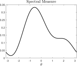
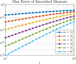
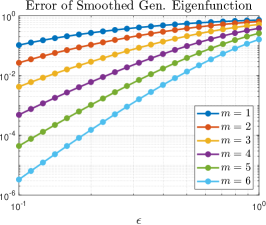
Figure 5: Left: The density of the spectral measure $\xi_{g}$ for the cat map example. Middle: The $L^{\infty}({[{-}\pi,\pi]_{\mathrm{per}}})$ error of the smoothed approximation computed using the kernels in Fig. 4. Right: The error of the smoothed generalized eigenfunctions of the cat map computed using Algorithm 1.

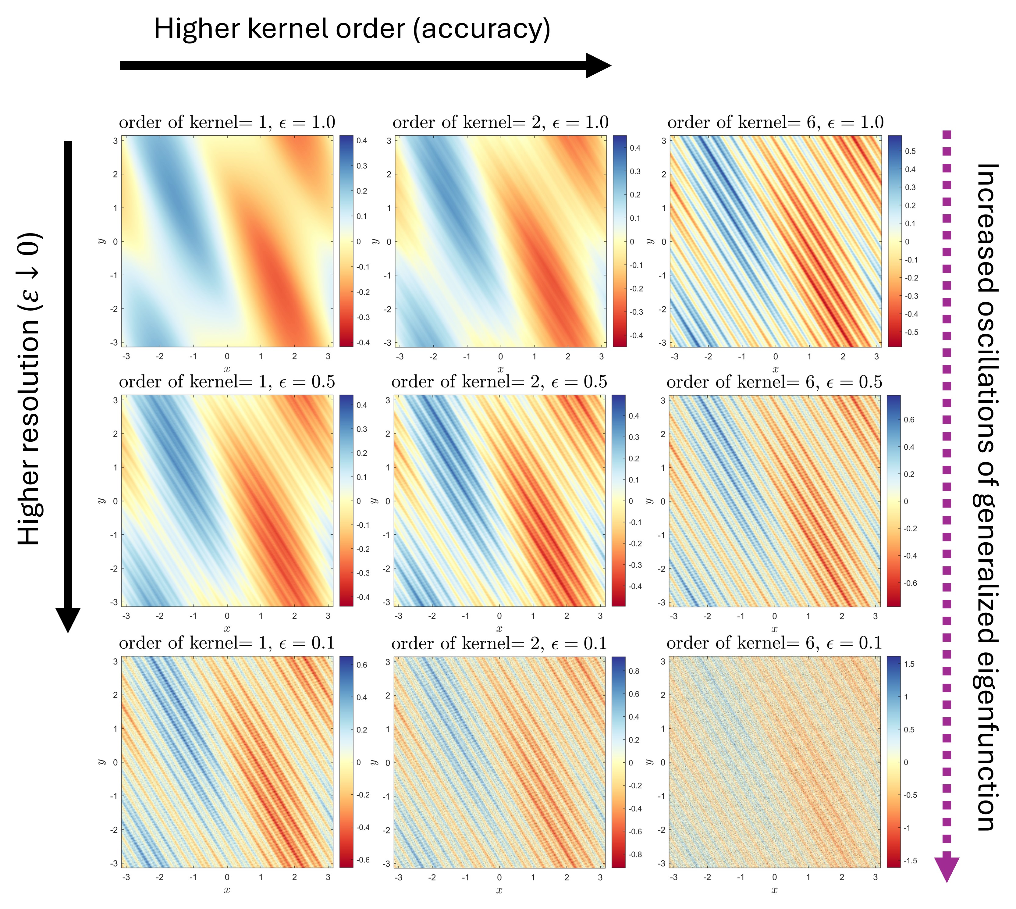
Figure 6: The smoothed generalized eigenfunctions of the cat map computed using Algorithm 1.

We collect data $\{\mathbf{x}^{(m)},\mathbf{y}^{(m)}\}$ along an equispaced $50\times 50$ grid for $\mathbf{x}^{(m)}$ over $\Omega$, corresponding to $M=2500$. As a dictionary, we employ time-delay embedding with the function

$$g=\sin(x)+\frac{1}{2}\sin(2x+y)+\frac{i}{4}\sin(5x+3y).$$

This function is chosen because we can analytically compute the spectral measure and generalized eigenfunctions. Fig. 5 shows the spectral measure and the maximum errors of the smoothed approximations computed using Algorithm 1. We see the convergence rates $\mathcal{O}(\epsilon^{m}{\log(1+\epsilon^{-1})})$ predicted by the theorems in Section 5.2. To demonstrate the convergence of the smoothed generalized eigenfunctions, we represent the eigenfunction at $\theta=1$ in the basis $\{g,\mathcal{K}g,\mathcal{K}^{2}g,\ldots\}$ and consider the relative $l^{2}$ norm error of the first five coefficients. These are also shown in Fig. 5 and again demonstrate the high-order convergence. Fig. 6 shows the corresponding smoothed generalized eigenfunctions. As $\epsilon\downarrow 0$, these functions become more oscillatory (as predicted by the above analysis). For the higher-order kernels, we see an increased resolution of the approximation for a given $\epsilon$.

7.2 Integrable Hamiltonian systems

The nonlinear pendulum has continuous spectra and is a well-known challenge for DMD methods [57]. We consider general integrable Hamiltonian systems, before specializing to this example. The Arnold–Liouville theorem states that if a Hamiltonian system with $n$ degrees of freedom has $n$ independent, Poisson commuting first integrals of motion, and if the constant energy manifolds are compact, then there exists a transformation to local action-angle coordinates in which (a) the transformed Hamiltonian is dependent only upon the action coordinates and (b) the angle coordinates evolve linearly in time [8]. Suppose that our system can be transformed to global action-angle coordinates $\mathbf{x}=(\mathbf{I},\bm{\theta})\in\mathbb{R}^{n}\times[-\pi,\pi]_{\mathrm{per}}^{n}=\Omega$ such that $\dot{\mathbf{I}}=0,\dot{\bm{\theta}}=\mathbf{I}$. We sample the continuous dynamical system at discrete time steps of $\Delta t>0$. The associated discrete dynamical system has the map $\mathbf{F}(\mathbf{I},\bm{\theta})=(\mathbf{I},\bm{\theta}+\Delta t\mathbf{I})$ and the Koopman operator is

$$[\mathcal{K}g](\mathbf{I},\bm{\theta})=g(\mathbf{I},\bm{\theta}+\Delta t\mathbf{I}),\qquad\text{where}\qquad g\in L^{2}(\Omega,\omega),$$

and $\omega$ is the Lebesgue measure normalized by $(2\pi)^{-n}$. We equip $L^{2}(\Omega,\omega)$ with the nuclear space $\mathcal{S}=S(\mathbb{R}^{n})\times C^{\infty}([-\pi,\pi]_{\mathrm{per}}^{n})$, where $S(\mathbb{R}^{n})$ denotes the Schwartz space on $\mathbb{R}^{n}$.

Given $g\in\mathcal{S}$, we denote the $n$-dimensional Fourier series in the angle coordinates of $g$ by

$$g(\mathbf{I},\bm{\theta})=\sum_{\mathbf{k}\in\mathbb{Z}^{n}}\hat{g}_{\mathbf{k}}(\mathbf{I})e^{i\mathbf{k}\cdot\bm{\theta}},\qquad\text{where}\qquad\hat{g}_{\mathbf{k}}(\mathbf{I})=\frac{1}{(2\pi)^{n}}\int_{[-\pi,\pi]_{\mathrm{per}}^{n}}g(\mathbf{I},\bm{\theta})e^{-i\mathbf{k}\cdot\bm{\theta}}{\,\mathrm{d}}{\bm{\theta}}.$$

In the Fourier basis for the angle coordinates, $\mathcal{K}$ acts as a multiplication operator, because

(30) $$\widehat{[\mathcal{K}g]}_{\mathbf{k}}(\mathbf{I})=\exp(-i\Delta t\mathbf{k}\cdot\mathbf{I})\hat{g}_{\mathbf{k}}(\mathbf{I}),\qquad\text{for each}\qquad\mathbf{k}\in\mathbb{Z}^{n}.$$

Examining the resolvent of this multiplication operator, it is straightforward to see that the spectrum of $\mathcal{K}$ is continuous for all $\lambda\in\mathbb{T}$ except for an eigenvalue of (countably) infinite multiplicity at $\lambda=1$, corresponding to observables with no angular dependence. We, therefore, study each Fourier mode separately.

When $\mathbf{k}=0$, the Koopman operators acts as the identity and, consequently, every angle-independent observable is an eigenfunction. Let $\{\phi_{j}\}_{j=1}^{\infty}\subset S(\mathbb{R}^{n})$ be an orthonormal basis of $L^{2}(\mathbb{R}^{n})$. The zeroth mode can be recovered by the generalized eigenfunction expansion

$$g_{0}(\mathbf{I})=\sum_{j=1}^{\infty}\underbrace{\int_{\mathbb{R}^{n}}g_{0}(\mathbf{I}^{\prime})\overline{\phi_{j}(\mathbf{I}^{\prime})}{\,\mathrm{d}}\mathbf{I}^{\prime}}_{=\langle\phi_{j}^{*}|g\rangle}\phi_{j}(\mathbf{I})=\sum_{j=1}^{\infty}\int_{[{-}\pi,\pi]_{\mathrm{per}}}\langle\phi_{j}^{*}|g\rangle\phi_{j}(\mathbf{I})\delta(\varphi){\,\mathrm{d}}\varphi.$$

When $\mathbf{k}\neq 0$ and $\tau\in\mathbb{R}$, we define the $(n-1)$-dimensional hyperplane

$$H_{\mathbf{k}}(\tau)=\{\mathbf{I}\in\mathbb{R}^{n}:\Delta t\mathbf{I}\cdot\mathbf{k}=\tau\},$$

and $Q_{\mathbf{k}}(\mathbf{I})$ the projection of $\mathbf{I}$ onto its component perpendicular to $\mathbf{k}$. The Koopman operator acts as multiplication by a constant along each hyperplane $H_{\mathbf{k}}(\tau)$ but is a nontrivial multiplication operator along their orthogonal complements. Let $\{\psi_{j}^{(\mathbf{k})}\}_{j=1}^{\infty}\subset S(H_{\mathbf{k}}(0))$ be an orthonormal basis of the space $L^{2}(H_{\mathbf{k}}(0))$ equipped with the standard surface measure $\sigma$. For $\lambda=e^{i\theta}\in\mathbb{T}$, $m\in\mathbb{Z}$ and $j\in\mathbb{N}$, we define the distribution $u_{\theta}^{(\mathbf{k},m,j)}$ via

(31) $$\left\langle{u_{\theta}^{(\mathbf{k},m,j)}}^{*}|g\right\rangle=\int_{H_{\mathbf{k}}(\theta+2\pi m)}\hat{g}_{\mathbf{k}}(\mathbf{I})\overline{\psi_{j}^{(\mathbf{k})}(Q_{\mathbf{k}}(\mathbf{I}))}{\,\mathrm{d}}\sigma(\mathbf{I}).$$

Using the relation (30), we see that $u_{\theta}^{(\mathbf{k},m,j)}$ is a generalized eigenfunction corresponding to $\lambda=e^{i\theta}$. Formally, we have

(32) $$u_{\theta}^{(\mathbf{k},m,j)}(\mathbf{I},\bm{\theta})=\frac{1}{(2\pi)^{n}}\delta(\theta+2\pi m-\Delta t\mathbf{k}\cdot\mathbf{I})\psi_{j}^{(\mathbf{k})}(Q_{\mathbf{k}}(\mathbf{I}))e^{i\mathbf{k}\cdot\bm{\theta}},$$

where the Dirac-delta distribution should be understood in terms of the integration along hyperplanes in Eq. 31. It is straightforward to show that

$$\hat{g}_{\mathbf{k}}(\mathbf{I})e^{i\mathbf{k}\cdot\bm{\theta}}=\sum_{m=-\infty}^{\infty}\sum_{j=1}^{\infty}\int_{[{-}\pi,\pi]_{\mathrm{per}}}\langle u_{\varphi}^{(\mathbf{k},m,j)*}|g\rangle u_{\varphi}^{(\mathbf{k},m,j)}(\mathbf{I},\bm{\theta}){\,\mathrm{d}}\varphi.$$

Hence, the Koopman mode decomposition of $g\in\mathcal{S}$ is

$$g(\mathbf{I},\bm{\theta})\!=\!\sum_{j=1}^{\infty}\!\int_{[{-}\pi,\pi]_{\mathrm{per}}}\!\!\!\langle\phi_{j}^{*}|g\rangle\phi_{j}(\mathbf{I})\delta(\varphi){\,\mathrm{d}}\varphi+\!\!\!\sum_{\mathbf{k}\in\mathbb{Z}^{n}\backslash\{0\}}\sum_{m=-\infty}^{\infty}\sum_{j=1}^{\infty}\int_{[{-}\pi,\pi]_{\mathrm{per}}}\!\!\!\langle u_{\varphi}^{(\mathbf{k},m,j)*}|g\rangle u_{\varphi}^{(\mathbf{k},m,j)}(\mathbf{I},\bm{\theta}){\,\mathrm{d}}\varphi.$$

In particular, the generalized eigenfunctions consist of eigenfunctions in the usual sense (in $L^{2}(\Omega,\omega)$) corresponding to $\lambda=1$ that depend only on $\mathbf{I}$, and generalized eigenfunctions of the form in Eq. 32 corresponding to any $\lambda\in\mathbb{T}$. These latter generalized eigenfunctions are plane waves with singular support along hyperplanes of constant directions of action.

7.2.1 Nonlinear pendulum

We consider the dynamical system of the nonlinear pendulum. The state variables $\mathbf{x}=(x_{1},x_{2})$ are governed by the following coupled ODEs:

$$\dot{x_{1}}=x_{2},\quad\dot{x_{2}}=-\sin(x_{1}),\quad\text{ with}\quad\Omega=[-\pi,\pi]_{\mathrm{per}}\times\mathbb{R},$$

where $\omega$ is the standard Lebesgue measure on $\Omega$. We consider the corresponding discrete-time dynamical system by sampling with a time-step $\Delta_{t}=1$. This system is Hamiltonian with one degree of freedom. A special case of the spectral decomposition we derived in Section 7.2 was derived in [64] for this system.

We employ time-delay embedding $\{g,\mathcal{K}g,\ldots,\mathcal{K}^{299}g\}$ with $g(x_{1},x_{2})=\exp(ix_{1})/\cosh(x_{2})$, and collect data on a 500-point equispaced grid in both $x_{1}$ and $x_{2}$ directions. Trajectory data is generated using MATLAB’s ode45, based on initial conditions from this grid. We apply a trapezoidal quadrature rule with super-algebraic convergence in mpEDMD [82, 80]. Figure 7 shows the spectral measure and generalized eigenfunctions computed using Rigged DMD with smoothing parameter $\epsilon=0.05$ and the $6$th order kernel from Fig. 4. The singular support and plane wave structure of the generalized eigenfunctions for $\lambda\neq 0$ are clearly visible.

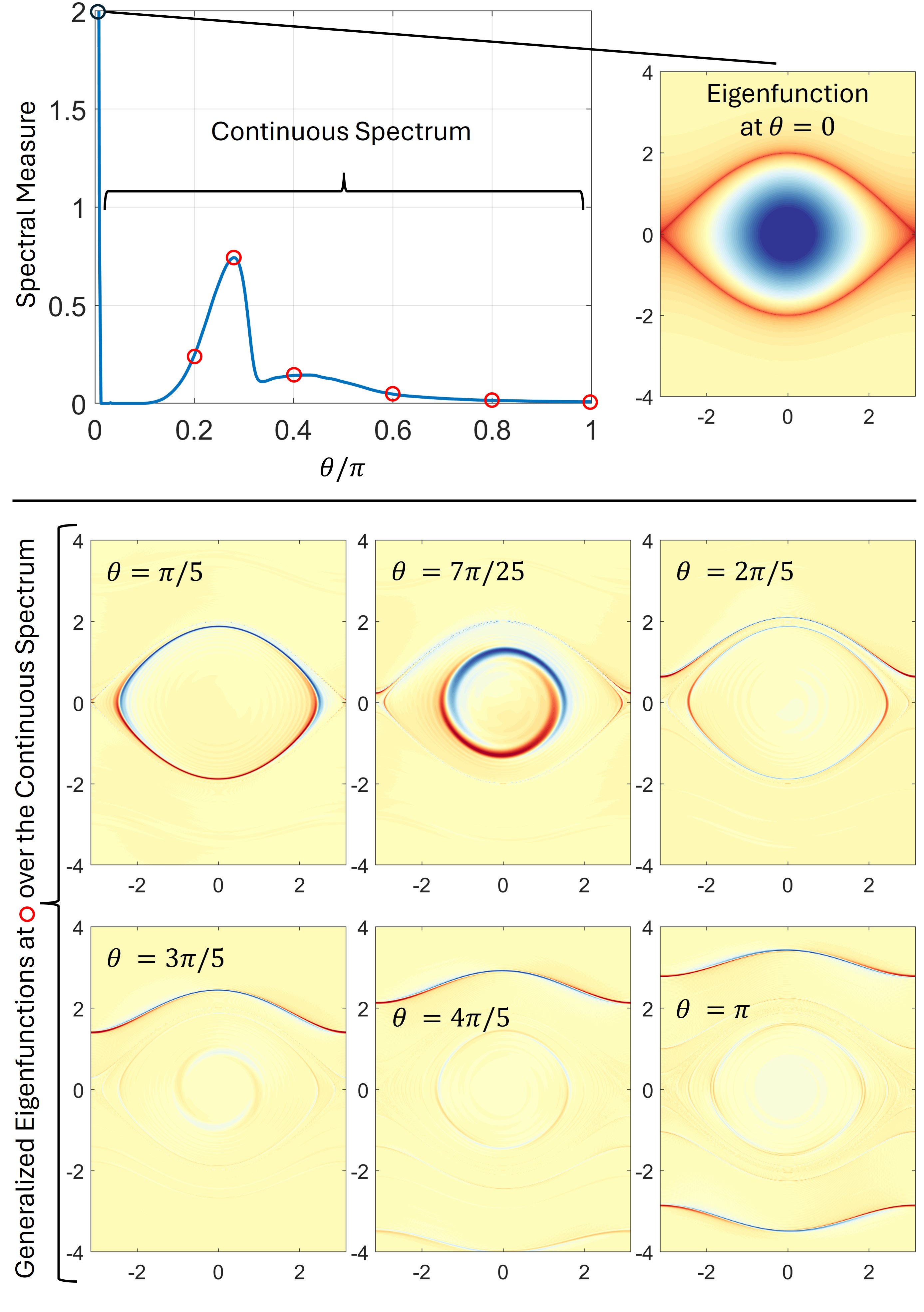
Figure 7: The smoothed generalized eigenfunctions of the nonlinear pendulum computed using Algorithm 1.

7.3 The Lorenz system

The Lorenz (63) system with classical parameter values [56] is the following three coupled ODEs:

$$\dot{x}=10\left(y-x\right),\quad\dot{y}=x\left(28-z\right)-y,\quad\dot{z}=xy-8z/3.$$

We consider the dynamics of $\mathbf{x}=(x,y,z)$ on the Lorenz attractor $\Omega$. This system has a unique SRB measure $\omega$ on $\Omega$ [84], meaning that for Lebesgue-almost every initial condition $\mathbf{x}_{0}$ in the basin of attraction of $\Omega$ and compactly supported function $g:\mathbb{R}^{3}\rightarrow\mathbb{C}$,

(33) $$\lim_{M\rightarrow\infty}\frac{1}{M}\sum_{m=0}^{M-1}[\mathcal{K}^{m}g](\mathbf{x}_{0})=\int_{\Omega}g(\mathbf{x}){\,\mathrm{d}}\omega(\mathbf{x}).$$

The system is chaotic and strong mixing [58]. It follows that $\lambda=1$ is the only eigenvalue of $\mathcal{K}$, corresponding to a constant eigenfunction, and that this eigenvalue is simple.

We consider a discrete-time dynamical system by sampling with a time-step $\Delta t=0.05$ and collecting $M=10^{4}$ snapshot pairs over a single trajectory. This quadrature rule is justified by Eq. 33. We use the ode45 command in MATLAB to collect the data after an initial burn-in time to ensure that the initial point $\mathbf{x}(0)$ is (approximately) on the Lorenz attractor. The system is chaotic, so we cannot hope to accurately numerically integrate for long periods. However, convergence is still obtained in the large data limit $M\rightarrow\infty$ due to an effect known as shadowing. As our dictionary, we use time delays of the function

$$\psi_{1}(\mathbf{x})=g(\mathbf{x})=\tanh((xy-5z)/10)-c,\quad\psi_{j}=\mathcal{K}^{j-1}g,\quad j=2,\ldots,N,$$

where $c$ is a constant chosen so that $g$ is orthogonal to the one-dimensional space spanned by constant functions. The value of $c\approx-0.5382$ is computed by taking the average of $\tanh((xy-5z)/10)$ over our trajectory. Shifting by $c$ ensures that the spectral measure $\xi_{g}$ is purely continuous. Fig. 2 shows the spectral measure computed using $N=1000$, the $6$th order kernel in Fig. 4 and a smoothing parameter $\epsilon=0.05$. There are four noticeable peaks at $\theta\approx 0.414,0.497,0.828,$ and $0.994$. Since the spectral measure is continuous, these do not correspond to eigenvalues. Instead, we can compute generalized eigenfunctions corresponding to these values to obtain approximately coherent structures. These are also shown in Fig. 2. The function labeled (a) is similar to the local spectral projections in [53, Figure 13] (see also [24, Figure 4]), which the authors attributed to an almost-periodic motion of the $z$ component during the time that the state resides in either of the two lobes of the Lorenz attractor. The function labeled (c) corresponds to double the angle $\theta$ of that of (a) and roughly the square of the corresponding function. The structures in (b) and (d) are different and include oscillations within each lobe.

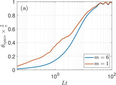
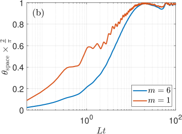
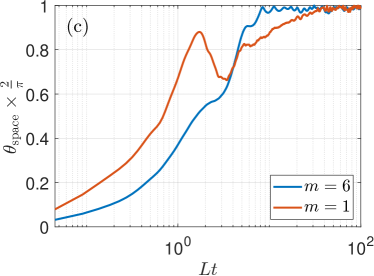
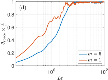
Figure 8: The subspace angle between $g_{\theta}^{\epsilon}$ and $\mathcal{K}^{n}g_{\theta}^{\epsilon}$, plotted against $Lt$ with $L$ the maximal Lyapunov exponent of the Lorenz system. The labels (a), (b), (c) and (d) correspond to Fig. 2. The angle $\theta_{\mathrm{space}}\in[0,\pi/2]$ measures the angle between subspaces, with a value of zero corresponding to perfect coherency and a value of $\pi/2$ corresponding to perfect incoherency.

To measure the coherency of each approximate generalized eigenfunction $g_{\theta}^{\epsilon}$, we measure the subspace angle between $g_{\theta}^{\epsilon}$ and $\mathcal{K}^{n}g_{\theta}^{\epsilon}$. We do this over a larger data set of $10^{5}$ trajectory points to ensure that the subspace angle is accurate and does not correspond to fitting our original snapshot data. Fig. 8 shows these angles, where we have plotted against $Lt$ with $L$ the maximal Lyapunov exponent of the Lorenz system. In agreement with Eq. 6 and Theorem 5.13, we see that our computed generalized eigenfunctions are highly coherent over several Lyapunov time scales. Moreover, higher-order kernels lead to larger levels of coherency.

7.4 Lid-driven cavity flow

As our final example, we consider a 2D lid-driven cavity flow at various Reynolds numbers. The flow is a simple model of an incompressible viscous fluid confined to a rectangular box with a moving lid and is a standard benchmark [83, 18, 54]. As the Reynolds number increases, the Koopman spectrum undergoes a series of bifurcations from pure point to mixed to pure continuous spectrum [73, 6]. It was also shown in [6, e.g., Figure 7] that for high Reynolds number, it is challenging to capture the flow with discrete DMD expansions. We use the data from [6], namely, the vorticity field within the cavity at $Re=13000$, $16000$, $19000$ and $30000$ collected over 10000 snapshots. We have also added 20% Gaussian random noise (SNR of 14) to demonstrate the robustness of Rigged DMD.

Fig. 9 shows the spectral measures of the total kinetic energy, computed using Algorithm 1 with a 10th order kernel, $\epsilon=0.001$ and a dictionary formed by time delays. At $Re=13000$, we see pure point spectrum built from a base frequency. As the Reynolds number increases, the spectrum becomes mixed and then continuous. Figs. 10, 11, 12 and 13 show the generalized Koopman modes computed using Algorithm 2 with a 6th order kernel and $\epsilon=0.01$ and a dictionary of $10$, $100$, $200$ and $500$ POD modes for $Re=13000$, $16000$, $19000$ and $30000$, respectively. As our values of $\theta$, we pick the Strouhal numbers corresponding to the four peaks visible in the spectral measure at $Re=13000$. We have shown the results with the noisy data and the noise-free data. As expected, larger frequencies are more affected by noise. Nevertheless, we are able to compute these modes over the continuous spectrum in the presence of large noise. There are three reasons for robustness of Rigged DMD. The first is that mpEDMD is equivalent to a constrained total least squares problem (see the discussion in [23, Section 6.2]). The second is the smoothing parameter (high-order kernels help, see the discussion in [28, Section 5.1.2]). The third is the averaging procedure in Algorithm 2.

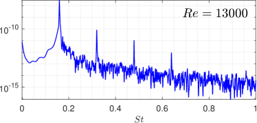
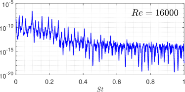
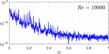
Figure 9: Spectral measures of the kinetic energy of the lid-driven cavity flow.

Figure 10: Generalized Koopman modes for the cavity flow at $Re=13000$.

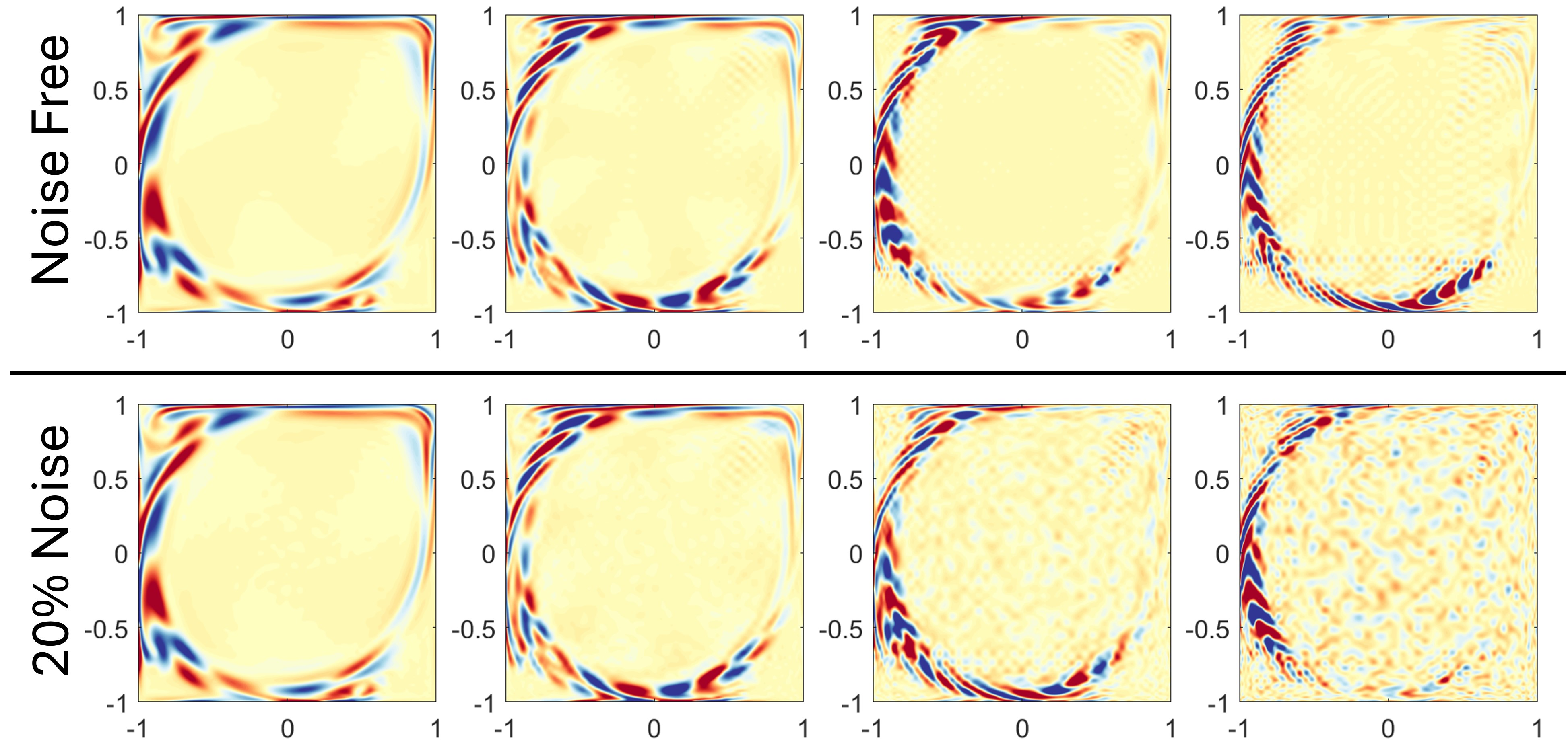
Figure 11: Generalized Koopman modes for the cavity flow at $Re=16000$.

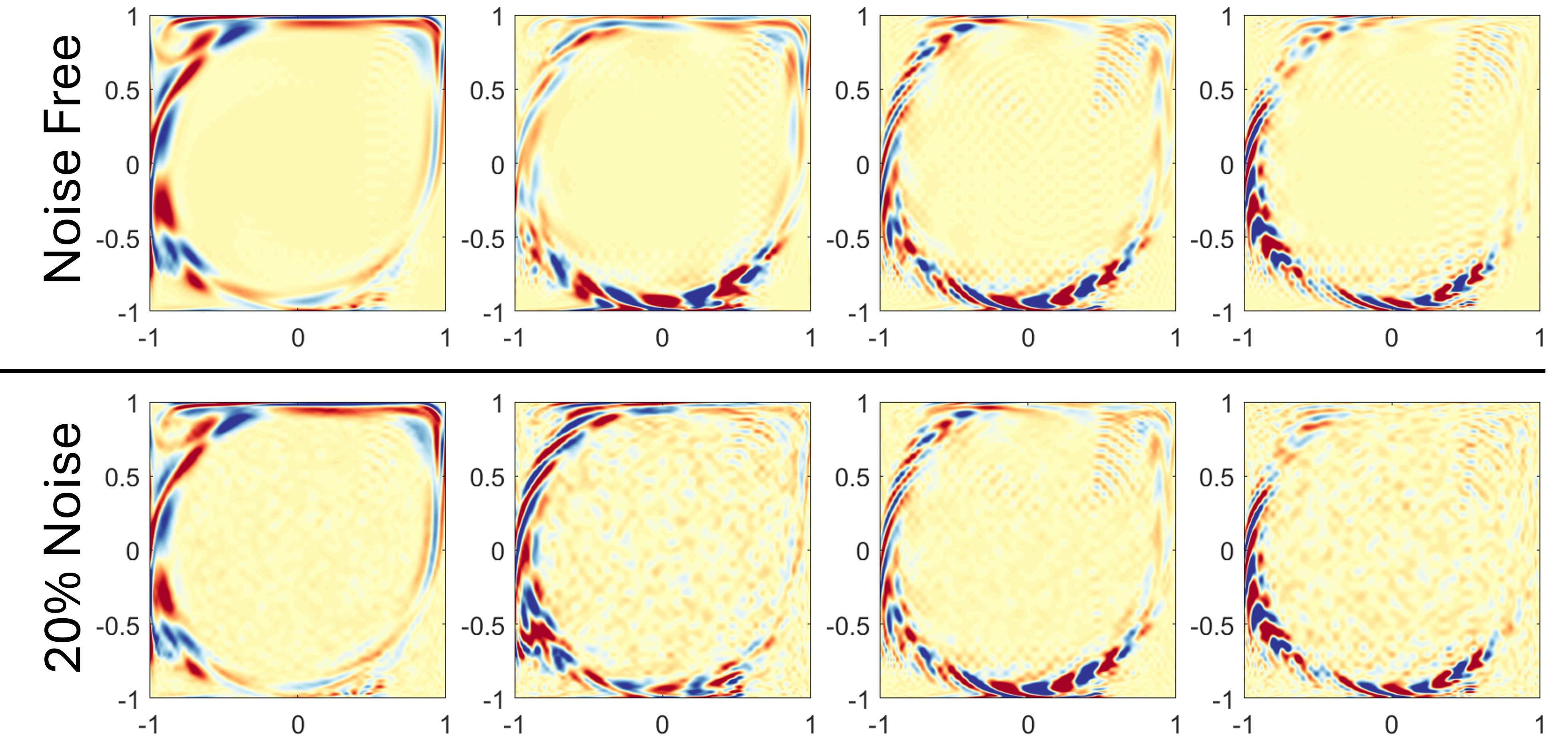
Figure 12: Generalized Koopman modes for the cavity flow at $Re=19000$.

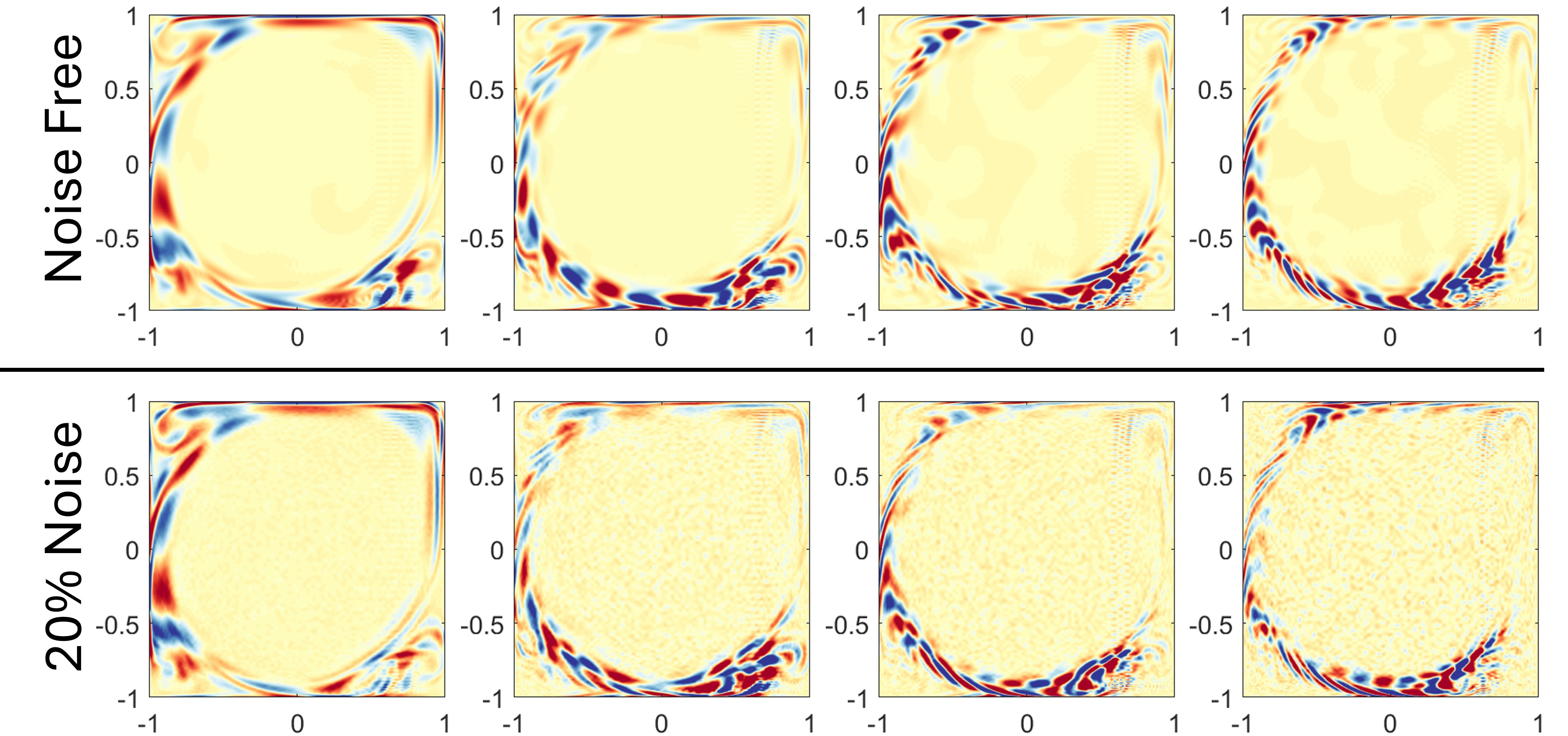
Figure 13: Generalized Koopman modes for the cavity flow at $Re=30000$.

8 Conclusions

We have developed an algorithm that computes generalized eigenfunction expansions (mode decompositions) of Koopman operators, even in the presence of continuous spectra. Named Rigged DMD, the algorithm leverages Gelfand’s theorem, which asserts that a complete set of generalized eigenfunctions exists within a rigged Hilbert space. Rigged DMD employs unitary approximations of Koopman operators, computed using mpEDMD, to determine the Koopman resolvent. This resolvent is then used to compute smoothed approximations of generalized eigenfunctions for any spectral parameter. We have not only shown examples of rigged Hilbert spaces but also demonstrated how to realize this assumption for general unitary Koopman operators using appropriately weighted vectors derived from delay embedding. In addition to proving convergence theorems for generalized eigenfunctions and spectral measures, we have demonstrated the algorithm’s applicability and robustness through several examples. There is considerable potential for future work, and we briefly discuss two avenues. The first involves applying Rigged DMD to reduced order models and control problems involving continuous spectra. Specifically, Rigged DMD opens the door to control over the interactions between modes corresponding to the continuous and discrete spectra. Second, we relied on the Koopman operator being unitary (i.e., the system is measure-preserving and invertible). We aim to extend Rigged DMD to non-unitary and non-normal Koopman operators, a development that would require adapting these techniques to scenarios where the nuclear spectral theorem does not apply.

Appendix A Strong convergence of the mpEDMD resolvent

To prove Theorem 4.1, we use the following lemma from [23]. We stress that the second part of the lemma need not hold for methods such as EDMD. In particular, convergence in the strong operator topology (the convergence of EDMD) need not imply convergence of adjoints in the strong operator topology, even if the desired limit is unitary. The polar decomposition in mpEDMD is crucial for strong convergence of the adjoint of the Koopman operator.

Lemma A.1.

Suppose that $\lim_{N\rightarrow\infty}\!\mathrm{dist}(h,V_{N})=0$ for all $h\in L^{2}(\Omega,\omega)$ and Eq. 15 holds. Then for any $g\in L^{2}(\Omega,\omega)$ and $\mathbf{g}_{N}\in\mathbb{C}^{N}$ with $\lim_{N\rightarrow\infty}\|g-\mathbf{\Psi}\mathbf{g}_{N}\|=0$,

(34) $$\lim_{N\rightarrow\infty}\limsup_{M\rightarrow\infty}\|\mathcal{K}^{l}g-\mathbf{\Psi}\mathbf{K}^{l}\mathbf{g}_{N}\| =0\quad\forall l\in\mathbb{N}\cup\{0\},$$

(35) $$\lim_{N\rightarrow\infty}\limsup_{M\rightarrow\infty}\|(\mathcal{K}^{*})^{l}g-\mathbf{\Psi}\mathbf{K}^{-l}\mathbf{g}_{N}\| =0\quad\forall l\in\mathbb{N}\cup\{0\}.$$

Proof A.2 (Proof of Theorem 4.1).

Suppose first that $|z|>1$. Since $\|\mathcal{K}\|=1$ and $\|\mathbf{G}^{1/2}\mathbf{K}\mathbf{G}^{-1/2}\|=1$,

$$(\mathcal{K}-zI)^{-1}g =\frac{-1}{z}(I-\mathcal{K}/z)^{-1}g=\frac{-1}{z}\sum_{l=0}^{\infty}\frac{1}{z^{l}}\mathcal{K}^{l}g$$

$$(\mathbf{K}-z\mathbf{I})^{-1}g =\frac{-1}{z}(\mathbf{I}-\mathbf{K}/z)^{-1}\mathbf{g}_{N}=\frac{-1}{z}\sum_{l=0}^{\infty}\frac{1}{z^{l}}\mathbf{K}^{l}\mathbf{g}_{N}.$$

The tails of these series can be uniformly bounded, and for any $l\in\mathbb{N}\cup\{0\}$, Eq. 34 implies that

$$\lim_{N\rightarrow\infty}\limsup_{M\rightarrow\infty}\left\|\frac{1}{z^{l}}\mathcal{K}^{l}g-\mathbf{\Psi}\frac{1}{z^{l}}\mathbf{K}^{l}\mathbf{g}_{N}\right\|=0.$$

The convergence in Eq. 17 now follows. Similarly, if $|z|<1$, we may write

$$(\mathcal{K}-zI)^{-1}g =(I-z\mathcal{K}^{*})^{-1}\mathcal{K}^{*}g=\sum_{l=0}^{\infty}z^{l}(\mathcal{K}^{*})^{l+1}g$$

$$(\mathbf{K}-z\mathbf{I})^{-1}g =(\mathbf{I}-z\mathbf{K}^{-1})^{-1}\mathbf{K}^{-1}\mathbf{g}_{N}=\sum_{l=0}^{\infty}{z^{l}}\mathbf{K}^{-l-1}\mathbf{g}_{N}.$$

We argue similarly using Eq. 35 to see that Eq. 17 holds.

Appendix B Construction of high-order periodic kernels

Proof B.1 (Proof of Proposition 5.5).

The decay condition Eq. 23 in Definition 5.4 ensures that the series defining $K_{\epsilon}^{\mathbb{T}}$ is absolutely convergent and hence that $K_{\epsilon}^{\mathbb{T}}$ is continuous. Similarly,

$$\int_{-\pi}^{\pi}K_{\epsilon}^{\mathbb{T}}(\theta){\,\mathrm{d}}\theta=\int_{\mathbb{R}}K_{\epsilon}(x){\,\mathrm{d}}x=1.$$

We may write

$$\int_{-\pi}^{\pi}K_{\epsilon}^{\mathbb{T}}(-\theta)e^{in\theta}{\,\mathrm{d}}\theta-1=\int_{\mathbb{R}}K_{\epsilon}(x)\left[e^{-inx}-1\right]{\,\mathrm{d}}x=[K_{\epsilon}\ast\rho](0),$$

where $\rho(x)=e^{inx}-1$. Since $\rho$ is a bounded, smooth function, and $\rho(0)=0$, we may apply [19, Theorem 5.2] to deduce that Eq. 21 holds.

We are left with proving the concentration bound Eq. 22. By directly plugging Eq. 23 into the definition of $K_{\epsilon}^{\mathbb{T}}$, we see that

(36) $$|K_{\epsilon}^{\mathbb{T}}(\theta)|\lesssim\frac{1}{\epsilon}\sum_{n\in\mathbb{Z}}\frac{1}{(1+\left|\theta+2\pi n\right|/\epsilon)^{m+1}}=\sum_{n\in\mathbb{Z}}\frac{\epsilon^{m}}{(\epsilon+|\theta+2\pi n|)^{m+1}}.$$

For any non-zero integer $n$, we have $|\theta+2\pi n|\geq\pi|n|$ and hence

$$\sum_{n\in\mathbb{Z}\backslash{\{0\}}}\frac{1}{(\epsilon+|\theta+2\pi n|)^{m+1}}\leq\sum_{n\in\mathbb{Z}\backslash{\{0\}}}\frac{1}{|\theta+2\pi n|^{m+1}}<\infty.$$

It follows that

$$|K_{\epsilon}^{\mathbb{T}}(\theta)|\lesssim\epsilon^{m}+\frac{\epsilon^{m}}{(\epsilon+|\theta|)^{m+1}},$$

where the second term on the right-hand side comes from the $n=0$ term in the series in Eq. 36. The decay condition Eq. 22 now follows.

Proof B.2 (Proof of Proposition 5.7).

The corresponding periodic kernel is given by

$$K_{\epsilon}^{\mathbb{T}}(\theta)=\frac{1}{2\pi i}\sum_{j=1}^{m}\sum_{n\in\mathbb{Z}}\left(\frac{\alpha_{j}}{\theta+2\pi n-\epsilon a_{j}}-\frac{\beta_{j}}{\theta+2\pi n-\epsilon b_{j}}\right),$$

where the rearrangement of the sum is justified by its absolute convergence. Since

$$\sum_{n\in\mathbb{Z}}\frac{1}{z+2\pi n}=\frac{1}{2}\cot\left(\frac{z}{2}\right)=\frac{-i}{2}\frac{1+e^{iz}}{1-e^{iz}},$$

the kernel can be re-written as

$$K_{\epsilon}^{\mathbb{T}}(\theta) \!=\!\frac{1}{2\pi i}\!\sum_{j=1}^{m}\left(\!\alpha_{j}\frac{1}{2}\cot\left(\frac{\theta-\epsilon a_{j}}{2}\right)\!-\!\beta_{j}\frac{1}{2}\cot\left(\frac{\theta-\epsilon b_{j}}{2}\right)\!\right)$$

$$\!=\!\frac{-1}{4\pi}\!\sum_{j=1}^{m}\!\left(\!\alpha_{j}\frac{1+e^{i\theta-i\epsilon a_{j}}}{1-e^{i\theta-i\epsilon a_{j}}}\!-\!\beta_{j}\frac{1+e^{i\theta-i\epsilon b_{j}}}{1-e^{i\theta-i\epsilon b_{j}}}\!\right)\!=\!\frac{-1}{4\pi}\!\sum_{j=1}^{m}\!\left(\!\alpha_{j}\frac{e^{-i\theta}+e^{-i\epsilon a_{j}}}{e^{-i\theta}-e^{-i\epsilon a_{j}}}\!-\!\beta_{j}\frac{e^{-i\theta}+e^{-i\epsilon b_{j}}}{e^{-i\theta}-e^{-i\epsilon b_{j}}}\!\right)\!\!.$$

The formula in Eq. 26 follows. If $b_{j}=\overline{a_{j}}$ and $\beta_{j}=\overline{\alpha_{j}}$, since $\langle F_{\mathcal{E}}(z)g,g\rangle=-\overline{\langle F_{\mathcal{E}}(1/\overline{z})g,g\rangle}$,

$$\left[K_{\epsilon}^{\mathbb{T}}\ast\xi_{g}\right](\theta_{0}) =\frac{-1}{2\pi}\sum_{j=1}^{m}{\rm Re}\left(\alpha_{j}\left\langle F_{\mathcal{E}}(e^{i\theta-i\epsilon a_{j}})g,g\right\rangle\right)$$

$$=\frac{-1}{2\pi}\sum_{j=1}^{m}{\rm Re}\left(\alpha_{j}\left\langle(\mathcal{K}-e^{i\theta-i\epsilon a_{j}}I)^{-1}g,(\mathcal{K}+e^{i\theta-i\epsilon a_{j}}I)^{*}g\right\rangle\right).$$

Appendix C Convergence of wave-packet approximations

We use the following notation throughout this section. Given $m\in\mathbb{N}$, we let $\{K_{\epsilon}^{\mathbb{T}}\}$ be an $m$th order kernel for ${[{-}\pi,\pi]_{\mathrm{per}}}$. Let $\mathcal{K}:\mathcal{H}\rightarrow\mathcal{H}$ be a unitary operator on a rigged Hilbert space $\mathcal{S}\subset\mathcal{H}\subset\mathcal{S}^{*}$ with $\mathcal{K}\mathcal{S}\subset\mathcal{S}$. Denote the absolutely continuous component of ${\rm Sp}(\mathcal{K})$ by ${\rm Sp}_{\rm ac}(\mathcal{K})$ and, given $g,\phi\in\mathcal{S}$, let $\rho_{g,\phi}$ be the Radon–Nikodym derivative of the absolutely continuous component of the spectral measure $\xi_{g,\phi}=\langle\mathcal{E}g,\phi\rangle$, with $\xi_{g}=\xi_{g,g}$ for brevity.

Before proving the main results, we note that the smoothed Koopman mode expansion in Eq. 28 can be simplified with, essentially, a “change-of-basis” for the generalized eigenspace:

(37) $$g_{\theta}^{\epsilon}=\int_{[{-}\pi,\pi]_{\mathrm{per}}}K_{\epsilon}(\theta-\varphi)\,\langle u_{\varphi}^{*}|g\rangle u_{\varphi}{\,\mathrm{d}}\xi_{g}(\varphi)\qquad\text{for every}\qquad g\in\mathcal{S},$$

where $u_{\theta}$ depends on $g$ and satisfies $\langle\mathcal{K}u_{\theta}|\phi\rangle=\lambda\langle\psi|\phi\rangle$ for all $\phi\in\mathcal{S}$ with $\lambda=\exp(i\theta)$. The action of $g_{\theta}^{\epsilon}$ on a function $f\in\mathcal{S}$ is given by

(38) $$\langle g_{\theta}^{\epsilon}|f\rangle=\int_{[{-}\pi,\pi]_{\mathrm{per}}}K_{\epsilon}(\theta-\varphi)\,\langle u_{\varphi}^{*}|g\rangle\langle u_{\varphi}|f\rangle{\,\mathrm{d}}\xi_{g}(\varphi)\qquad\text{for every}\qquad g\in\mathcal{S}.$$

The corresponding expansion of the spectral measure in the rigged Hilbert space is

(39) $$[\mathcal{E}(S)]g=\int_{S}\langle u_{\varphi}^{*}|g\rangle u_{\varphi}{\,\mathrm{d}}\xi_{g}(\varphi)\qquad\forall g\in\mathcal{S}.$$

After taking an inner product with $g$, Eq. 39 implies that

$$\xi_{g}(S)=\langle[\mathcal{E}(S)]g,g\rangle=\langle[\mathcal{E}(S)]g|\overline{g}\rangle=\int_{S}\langle u_{\varphi}^{*}|g\rangle\langle u_{\varphi}|\overline{g}\rangle{\,\mathrm{d}}\xi_{g}(\varphi)=\int_{S}|\langle u_{\varphi}^{*}|g\rangle|^{2}{\,\mathrm{d}}\xi_{g}(\varphi).$$

It follows that $|\langle u_{\varphi}^{*}|g\rangle|^{2}=1$ $\xi_{g}$-almost everywhere. We can, without loss of generality, scale each generalized eigenfunction by a phase factor so that $\langle u_{\varphi}^{*}|g\rangle=1$. As a consequence of this convention, upon taking an inner product with $f\in\mathcal{S}$, we see that $\smash{{\,\mathrm{d}}\xi_{g,f}(\varphi)=\langle u_{\varphi}|\overline{f}\rangle{\,\mathrm{d}}\xi_{g}(\varphi)}$.

Proof C.1 (Proof of Theorem 5.9).

Since the spectrum of $\mathcal{K}$ is absolutely continuous on the interval $\mathcal{I}$, the arguments above show that $\rho_{g,\phi}(\varphi)=\rho_{g}(\varphi)\langle u_{\varphi}|\overline{\phi}\rangle$ for $\varphi\in\mathcal{I}$. Theorem 5.9 now follows by applying Theorem 5.17 to the complex Borel measure $\xi_{g,{\phi}}$ after substitution in Eq. 38.

Proof C.2 (Proof of Theorem 5.11).

Under the hypotheses of the theorem, the integrand of Eq. 37 is equivalent to convolution with a complex Borel measure (with finite total variation) on ${[{-}\pi,\pi]_{\mathrm{per}}}$ for each point $\mathbf{x}\in\mathcal{A}$. The uniform integrability and continuity assumptions ensure that the total variation and Hölder norms are bounded independently of $\mathbf{x}\in\mathcal{A}$. Theorem 5.11 now follows from Theorem 5.17.

We now prove the convergence of the approximate eigenvector sequence.

Proof C.3 (Proof of Theorem 5.13).

Using the functional calculus, we have.

$$(\mathcal{K}-e^{i\theta_{0}}I)g_{\theta_{0}}^{\epsilon}=\left[\int_{{[{-}\pi,\pi]_{\mathrm{per}}}}(e^{i\varphi}-e^{i\theta_{0}})K_{\epsilon}^{\mathbb{T}}(\theta_{0}-\varphi){\,\mathrm{d}}\mathcal{E}(\varphi)\right]g.$$

This implies that

$$\|(\mathcal{K}-e^{i\theta_{0}}I)g_{\theta_{0}}^{\epsilon}\|^{2}=\int_{{[{-}\pi,\pi]_{\mathrm{per}}}}|e^{i\varphi}-e^{i\theta_{0}}|^{2}|K_{\epsilon}^{\mathbb{T}}(\theta_{0}-\varphi)|^{2}{\,\mathrm{d}}\xi_{g}(\varphi).$$

Similarly, we have

$$\|g_{\theta_{0}}^{\epsilon}\|^{2}=\int_{{[{-}\pi,\pi]_{\mathrm{per}}}}|K_{\epsilon}^{\mathbb{T}}(\theta_{0}-\varphi)|^{2}{\,\mathrm{d}}\xi_{g}(\varphi).$$

Suppose that $\epsilon\eta<\delta$ and let

$$I_{\delta}=\int_{|\theta_{0}-\varphi|\leq\delta}|K_{\epsilon}^{\mathbb{T}}(\theta_{0}-\varphi)|^{2}{\,\mathrm{d}}\xi_{g}(\varphi)\geq\left(\inf_{|\theta|<\eta\epsilon}{\epsilon|K_{\epsilon}^{\mathbb{T}}(\theta)|}\right)^{2}\frac{1}{\epsilon^{2}}\int_{|\theta_{0}-\varphi|\leq\eta\epsilon}1{\,\mathrm{d}}\xi_{g}(\varphi).$$

The two bounds in Theorem 5.13 imply that $\liminf_{\epsilon\downarrow 0}I_{\delta}>0$. We have

$$\int_{{[{-}\pi,\pi]_{\mathrm{per}}}}|e^{i\varphi}-e^{i\theta_{0}}|^{2}|K_{\epsilon}^{\mathbb{T}}(\theta_{0}-\varphi)|^{2}{\,\mathrm{d}}\xi_{g}(\varphi)$$

$$\quad\quad\quad\leq\left(\sup_{|\theta|\leq\delta}|1-e^{i\theta}|^{2}\right)I_{\delta}+\int_{|\theta_{0}-\varphi|>\delta}|e^{i\varphi}-e^{i\theta_{0}}|^{2}|K_{\epsilon}^{\mathbb{T}}(\theta_{0}-\varphi)|^{2}{\,\mathrm{d}}\xi_{g}(\varphi)$$

$$\quad\quad\quad\lesssim\delta^{2}I_{\delta}+\int_{|\theta_{0}-\varphi|>\delta}|e^{i\varphi}-e^{i\theta_{0}}|^{2}|K_{\epsilon}^{\mathbb{T}}(\theta_{0}-\varphi)|^{2}{\,\mathrm{d}}\xi_{g}(\varphi).$$

Using the concentration condition in Eq. 22, we see that

$$\lim_{\epsilon\downarrow 0}\int_{|\theta_{0}-\varphi|>\delta}|e^{i\varphi}-e^{i\theta_{0}}|^{2}|K_{\epsilon}^{\mathbb{T}}(\theta_{0}-\varphi)|^{2}{\,\mathrm{d}}\xi_{g}(\varphi)=0.$$

Similarly, we have

$$\int_{{[{-}\pi,\pi]_{\mathrm{per}}}}|K_{\epsilon}^{\mathbb{T}}(\theta_{0}-\varphi)|^{2}{\,\mathrm{d}}\xi_{g}(\varphi)\geq I_{\delta}-\int_{|\theta_{0}-\varphi|>\delta}|K_{\epsilon}^{\mathbb{T}}(\theta_{0}-\varphi)|^{2}{\,\mathrm{d}}\xi_{g}(\varphi)$$

and

$$\lim_{\epsilon\downarrow 0}\int_{|\theta_{0}-\varphi|>\delta}|K_{\epsilon}^{\mathbb{T}}(\theta_{0}-\varphi)|^{2}{\,\mathrm{d}}\xi_{g}(\varphi)=0.$$

Hence,

$$\limsup_{\epsilon\downarrow 0}\frac{\|(\mathcal{K}-e^{i\theta_{0}}I)g_{\theta_{0}}^{\epsilon}\|^{2}}{\|g_{\theta_{0}}^{\epsilon}\|^{2}}\lesssim\limsup_{\epsilon\downarrow 0}\frac{\delta^{2}I_{\delta}+\int_{|\theta_{0}-\varphi|>\delta}|e^{i\varphi}-e^{i\theta_{0}}|^{2}|K_{\epsilon}^{\mathbb{T}}(\theta_{0}-\varphi)|^{2}{\,\mathrm{d}}\xi_{g}(\varphi)}{I_{\delta}-\int_{|\theta_{0}-\varphi|>\delta}|K_{\epsilon}^{\mathbb{T}}(\theta_{0}-\varphi)|^{2}{\,\mathrm{d}}\xi_{g}(\varphi)}=\delta^{2}.$$

Since $\delta>0$ was arbitrary, the result now follows.

Proof C.4 (Proof of Theorem 5.15).

Taking $\mathcal{P}_{e^{i\theta_{0}}}=0$ in the case that $e^{i\theta_{0}}$ is not an eigenvalue,

$$\frac{1}{K_{\epsilon}^{\mathbb{T}}(0)}[K_{\epsilon}^{\mathbb{T}}\ast\mathcal{E}](\theta_{0})\mathcal{P}_{e^{i\theta_{0}}}g=\frac{1}{K_{\epsilon}^{\mathbb{T}}(0)}\int_{{[{-}\pi,\pi]_{\mathrm{per}}}}K_{\epsilon}^{\mathbb{T}}(\theta_{0}-\varphi){\,\mathrm{d}}\mathcal{E}(\varphi)\mathcal{P}_{e^{i\theta_{0}}}g=\mathcal{P}_{e^{i\theta_{0}}}g.$$

It follows that we can define

$$g_{\epsilon}^{\prime}=\frac{1}{K_{\epsilon}^{\mathbb{T}}(0)}[K_{\epsilon}^{\mathbb{T}}\ast\mathcal{E}](\theta_{0})g-\mathcal{P}_{e^{i\theta_{0}}}g=\frac{1}{K_{\epsilon}^{\mathbb{T}}(0)}[K_{\epsilon}^{\mathbb{T}}\ast\mathcal{E}](\theta_{0})(g-\mathcal{P}_{e^{i\theta_{0}}}g).$$

From the functional calculus, we have

(40) $$\|g_{\epsilon}^{\prime}\|^{2}=\int_{{[{-}\pi,\pi]_{\mathrm{per}}}}\frac{|K_{\epsilon}^{\mathbb{T}}(\theta_{0}-\varphi)|^{2}}{|K_{\epsilon}^{\mathbb{T}}(0)|^{2}}{\,\mathrm{d}}\xi_{g-\mathcal{P}_{e^{i\theta_{0}}}g}(\varphi).$$

The concentration bound in Eq. 22 and the condition $\liminf_{\epsilon\downarrow 0}{\epsilon|K_{\epsilon}^{\mathbb{T}}(0)|}>0.$ imply that

$$\frac{|K_{\epsilon}^{\mathbb{T}}(\theta_{0}-\varphi)|^{2}}{|K_{\epsilon}^{\mathbb{T}}(0)|^{2}}\lesssim\frac{1}{\epsilon^{2}|K_{\epsilon}^{\mathbb{T}}(0)|^{2}}\frac{1}{(1+|\theta_{0}-\varphi|/\epsilon|)^{2m+2}}.$$

is uniformly bounded and converges to zero as $\epsilon\downarrow 0$ whenever $\varphi\neq\theta_{0}$. Since $\xi_{g-\mathcal{P}_{e^{i\theta_{0}}}g}(\{\theta_{0}\})=0$, we can apply the dominated convergence theorem to the right-hand side of (40) to see that $\lim_{\epsilon\downarrow}\|g_{\epsilon}^{\prime}\|^{2}=0$, which proves the result.

Appendix D Construction of a rigged Hilbert spaces for sparse unitary operators

Proof D.1 (Proof of Lemma 6.1).

Let $\{e_{n}:n\in\mathbb{N}\}$ denote the canonical basis for $\ell^{2}(\mathbb{N})$. Then, for any weight function $\rho$, the vectors $\{e_{n}/\sqrt{\rho(n)}:n\in\mathbb{N}\}$ form an orthonormal basis of $l^{2}_{\rho}(\mathbb{N})$. We may represent the inclusion map $\iota$ as

$$\iota u=\sum_{j=1}^{\infty}\sqrt{\frac{\tau(j)}{\tau^{\prime}(j)}}\left\langle u,\frac{e_{j}}{\sqrt{\tau^{\prime}(j)}}\right\rangle_{\tau^{\prime}}\frac{e_{j}}{\sqrt{\tau(j)}}.$$

It follows that if

(41) $$\sum_{j=1}^{\infty}\sqrt{\frac{\tau(j)}{\tau^{\prime}(j)}}<\infty,$$

then $\iota$ is nuclear. To achieve part (ii), it is enough to consider finite linear combinations of the basis vectors $\{e_{n}/\sqrt{\tau^{\prime}(n)}:n\in\mathbb{N}\}$ of $l^{2}_{\tau^{\prime}}(\mathbb{N})$. Let $u=\sum_{j=1}^{N}u_{j}e_{j}.$ Then

$$\|u\|_{\tau^{\prime}}^{2}=\sum_{j=1}^{N}|u_{j}|^{2}\tau^{\prime}(j),\qquad\|Au\|_{\tau}^{2}=\sum_{j=1}^{N}|(Au)_{j}|^{2}\tau(j).$$

The assumption that $A$ is sparse implies that there exists an increasing function $f:\mathbb{N}\rightarrow\mathbb{N}$ with $f(n)\geq n$ such that $A_{jk}=0$ if $j>f(k)$ and hence we can write

$$(Au)_{j}=\sum_{k\in\{1,\ldots,N\},f(k)\geq j}A_{jk}u_{k}.$$

Hence by Hölder’s inequality,

$$|(Au)_{j}|^{2}\leq\sum_{k\in\{1,\ldots,N\},f(k)\geq j}|A_{jk}|^{2}\sum_{k\in\{1,\ldots,N\},f(k)\geq j}|u_{k}|^{2}\leq\|A^{*}\|^{2}\sum_{k\in\{1,\ldots,N\},f(k)\geq j}|u_{k}|^{2}.$$

Since $A$ is unitary on $l^{2}(\mathbb{N})$, $\|A^{*}\|=1$. It follows that

$$\|Au\|_{\tau}^{2}\leq\sum_{j=1}^{N}\sum_{k\in\{1,\ldots,N\},f(k)\geq j}|u_{k}|^{2}\tau(j)=\sum_{k=1}^{N}|u_{k}|^{2}\sum_{j=1}^{f(k)}\tau(j).$$

It follows that if

(42) $$\sum_{j=1}^{f(k)}\tau(j)\leq\tau^{\prime}(k),$$

then $\|Au\|_{\tau}\leq\|u\|_{\tau^{\prime}}$. To finish the proof, we select $\tau^{\prime}$ so that both Eq. 41 and Eq. 42 hold.

References

- [1] I. Antoniou, L. Dmitrieva, Y. Kuperin, and Y. Melnikov, Resonances and the extension of dynamics to rigged Hilbert space, Computers & Mathematics with Applications, 34 (1997), pp. 399–425.
- [2] I. Antoniou, B. Qiao, and Z. Suchanecki, Generalized spectral decomposition and intrinsic irreversibility of the Arnold Cat Map, Chaos, Solitons & Fractals, 8 (1997), pp. 77–90.
- [3] I. Antoniou and S. Tasaki, Generalized spectral decompositions of mixing dynamical systems, International Journal of Quantum Chemistry, 46 (1993), pp. 425–474.
- [4] I. Antoniou and S. Tasaki, Spectral decomposition of the Renyi map, Journal of Physics A: Mathematical and General, 26 (1993), p. 73.
- [5] H. Arbabi and I. Mezić, Ergodic theory, dynamic mode decomposition, and computation of spectral properties of the Koopman operator, SIAM Journal on Applied Dynamical Systems, 16 (2017), pp. 2096–2126, https://doi.org/10.1137/17m1125236.
- [6] H. Arbabi and I. Mezić, Study of dynamics in post-transient flows using Koopman mode decomposition, Physical Review Fluids, 2 (2017), p. 124402, https://doi.org/10.1103/physrevfluids.2.124402.
- [7] V. I. Arnold, Mathematical Methods of Classical Mechanics, Springer New York, 1989, https://doi.org/10.1007/978-1-4757-2063-1.
- [8] V. I. Arnol’d, Mathematical methods of classical mechanics, vol. 60, Springer Science & Business Media, 2013.
- [9] V. I. Arnold and A. Avez, Ergodic problems of classical mechanics, (No Title), (1968).
- [10] O. F. Bandtlow, I. Antoniou, and Z. Suchanecki, Resonances of dynamical systems and Fredholm-Riesz operators on rigged Hilbert spaces, Computers & Mathematics with Applications, 34 (1997), pp. 95–102.
- [11] O. F. Bandtlow, W. Just, and J. Slipantschuk, EDMD for expanding circle maps and their complex perturbations, arXiv preprint arXiv:2308.01467, (2023), https://doi.org/10.48550/ARXIV.2308.01467, https://arxiv.org/abs/2308.01467.
- [12] Y. M. Berezanskii, Expansions in eigenfunctions of selfadjoint operators, transl. math, Monographs AMS, 17 (1968).
- [13] A. Bohm, J. D. Dollard, and M. Gadella, Dirac Kets, Gamow Vectors and Gel’fand Triplets: The Rigged Hilbert Space Formulation of Quantum Mechanics Lectures in Mathematical Physics at the University of Texas at Austin, Springer, 1989.
- [14] F. E. Browder, The eigenfunction expansion theorem for the general self-adjoint singular elliptic partial differential operator. i. the analytical foundation, Proceedings of the National Academy of Sciences, 40 (1954), pp. 454–459.
- [15] S. L. Brunton, B. W. Brunton, J. L. Proctor, E. Kaiser, and J. N. Kutz, Chaos as an intermittently forced linear system, Nature Communications, 8 (2017), pp. 1–9, https://doi.org/10.1038/s41467-017-00030-8.
- [16] S. L. Brunton, M. Budišić, E. Kaiser, and J. N. Kutz, Modern Koopman theory for dynamical systems, SIAM Review, 64 (2022), pp. 229–340, https://doi.org/10.1137/21m1401243.
- [17] M. Budišić, R. Mohr, and I. Mezić, Applied Koopmanism, Chaos: An Interdisciplinary Journal of Nonlinear Science, 22 (2012), p. 047510, https://doi.org/10.1063/1.4772195.
- [18] R. Chella and J. M. Ottino, Fluid mechanics of mixing in a single-screw extruder, Industrial & engineering chemistry fundamentals, 24 (1985), pp. 170–180.
- [19] M. Colbrook, A. Horning, and A. Townsend, Computing spectral measures of self-adjoint operators, SIAM Review, 63 (2021), pp. 489–524, https://doi.org/10.1137/20m1330944.
- [20] M. J. Colbrook, The Foundations of Infinite-Dimensional Spectral Computations, PhD thesis, University of Cambridge, 2020.
- [21] M. J. Colbrook, Computing spectral measures and spectral types, Communications in Mathematical Physics, 384 (2021), pp. 433–501, https://doi.org/10.1007/s00220-021-04072-4.
- [22] M. J. Colbrook, On the computation of geometric features of spectra of linear operators on Hilbert spaces, Foundations of Computational Mathematics, (2022), pp. 1–82, https://doi.org/10.1007/s10208-022-09598-0.
- [23] M. J. Colbrook, The mpEDMD algorithm for data-driven computations of measure-preserving dynamical systems, SIAM Journal on Numerical Analysis, 61 (2023), pp. 1585–1608, https://doi.org/10.1137/22m1521407.
- [24] M. J. Colbrook, The multiverse of dynamic mode decomposition algorithms, arXiv preprint arXiv:2312.00137, (2023).
- [25] M. J. Colbrook, L. J. Ayton, and M. Szőke, Residual dynamic mode decomposition: Robust and verified Koopmanism, Journal of Fluid Mechanics, 955 (2023), p. A21, https://doi.org/10.1017/jfm.2022.1052.
- [26] M. J. Colbrook and A. C. Hansen, The foundations of spectral computations via the solvability complexity index hierarchy, Journal of the European Mathematical Society, 25 (2022), pp. 4639–4728, https://doi.org/10.4171/jems/1289.
- [27] M. J. Colbrook, B. Roman, and A. C. Hansen, How to compute spectra with error control, Physical Review Letters, 122 (2019), p. 250201, https://doi.org/10.1103/physrevlett.122.250201.
- [28] M. J. Colbrook and A. Townsend, Rigorous data-driven computation of spectral properties of Koopman operators for dynamical systems, Communications on Pure and Applied Mathematics, 77 (2023), pp. 221–283, https://doi.org/10.1002/cpa.22125.
- [29] J. B. Conway, A course in functional analysis, vol. 96, Springer New York, 2 ed., 2007, https://doi.org/10.1007/978-1-4757-4383-8.
- [30] I. P. Cornfeld, S. V. Fomin, and Y. G. Sinai, Ergodic theory, vol. 245, Springer Science & Business Media, 2012.
- [31] S. Das and D. Giannakis, Delay-coordinate maps and the spectra of Koopman operators, Journal of Statistical Physics, 175 (2019), pp. 1107–1145, https://doi.org/10.1007/s10955-019-02272-w.
- [32] S. Das, D. Giannakis, and J. Slawinska, Reproducing kernel Hilbert space compactification of unitary evolution groups, Applied and Computational Harmonic Analysis, 54 (2021), pp. 75–136, https://doi.org/10.1016/j.acha.2021.02.004.
- [33] M. Dörfle, Spectrum and eigenfunctions of the Frobenius-Perron operator of the tent map, Journal of statistical physics, 40 (1985), pp. 93–132.
- [34] B. A. Dubrovin, A. T. Fomenko, and S. P. Novikov, Modern Geometry - Methods and Applications Part I. The Geometry of Surfaces, Transformation Groups, and Fields, vol. 104, Springer New York, 1984, https://doi.org/10.1007/978-1-4684-9946-9.
- [35] T. Eisner, B. Farkas, M. Haase, and R. Nagel, Operator theoretic aspects of ergodic theory, vol. 272, Springer International Publishing, 2015, https://doi.org/10.1007/978-3-319-16898-2.
- [36] M. Gadella and F. Gómez, A measure-theoretical approach to the nuclear and inductive spectral theorems, Bulletin des sciences mathematiques, 129 (2005), pp. 567–590.
- [37] P. Gaspard, Diffusion, effusion, and chaotic scattering: An exactly solvable liouvillian dynamics, Journal of statistical physics, 68 (1992), pp. 673–747.
- [38] P. Gaspard, r-adic one-dimensional maps and the Euler summation formula, Journal of Physics A: Mathematical and General, 25 (1992), p. L483.
- [39] I. M. Gelfand and S. V. Fomin, Geodesic flows on manifolds of constant negative curvature, Uspekhi Matematicheskikh Nauk, 7 (1952), pp. 118–137.
- [40] I. M. Gelfand and A. G. Kostyuchenko, Generalized eigenfunction decompositions of differential and other operators, Dokl. Akad. Nauk SSSR, 103 (1955), pp. 349–352.
- [41] I. M. Gelfand and N. Y. Vilenkin, Generalized Functions, Volume 4: Applications of Harmonic Analysis, Academic Press, 1964.
- [42] N. Govindarajan, R. Mohr, S. Chandrasekaran, and I. Mezić, On the approximation of Koopman spectra for measure preserving transformations, SIAM Journal on Applied Dynamical Systems, 18 (2019), pp. 1454–1497, https://doi.org/10.1137/18m1175094.
- [43] N. Govindarajan, R. Mohr, S. Chandrasekaran, and I. Mezic, On the approximation of Koopman spectra of measure-preserving flows, SIAM Journal on Applied Dynamical Systems, 20 (2021), pp. 232–261, https://doi.org/10.1137/19m1282908.
- [44] H. H. Hasegawa and D. J. Driebe, Spectral determination and physical conditions for a class of chaotic piecewise-linear maps, Physics Letters A, 176 (1993), pp. 193–201.
- [45] H. H. Hasegawa and W. C. Saphir, Decaying eigenstates for simple chaotic systems, Physics Letters A, 161 (1992), pp. 471–476.
- [46] T. L. Hill, An introduction to statistical thermodynamics, Courier Corporation, 1986.
- [47] M. Kamb, E. Kaiser, S. L. Brunton, and J. N. Kutz, Time-delay observables for Koopman: Theory and applications, SIAM Journal on Applied Dynamical Systems, 19 (2020), pp. 886–917, https://doi.org/10.1137/18m1216572.
- [48] H. Kantz and T. Schreiber, Nonlinear time series analysis, Cambridge nonlinear science series, Cambridge Univ. Press, Cambridge, second edition ed., 2006.
- [49] T. Kato and S. T. Kuroda, Theory of simple scattering and eigenfunction expansions, in Functional Analysis and Related Fields: Proceedings of a Conference in honor of Professor Marshall Stone, held at the University of Chicago, May 1968, Springer, 1970, pp. 99–131.
- [50] Y. Katznelson, An Introduction to Harmonic Analysis, Cambridge University Press, 2004, https://doi.org/10.1017/cbo9781139165372.
- [51] B. O. Koopman, Hamiltonian systems and transformation in Hilbert space, Proceedings of the National Academy of Sciences, 17 (1931), pp. 315–318, https://doi.org/10.1073/pnas.17.5.315.
- [52] B. O. Koopman and J. von Neumann, Dynamical systems of continuous spectra, Proceedings of the National Academy of Sciences, 18 (1932), pp. 255–263, https://doi.org/10.1073/pnas.18.3.255.
- [53] M. Korda, M. Putinar, and I. Mezić, Data-driven spectral analysis of the Koopman operator, Applied and Computational Harmonic Analysis, 48 (2020), pp. 599–629, https://doi.org/10.1016/j.acha.2018.08.002.
- [54] J. Koseff and R. Street, The lid-driven cavity flow: a synthesis of qualitative and quantitative observations, (1984).
- [55] N. Kryloff and N. Bogoliouboff, La théorie générale de la mesure dans son application à l’étude des systèmes dynamiques de la mécanique non linéaire, The Annals of Mathematics, 38 (1937), pp. 65–113, https://doi.org/10.2307/1968511.
- [56] E. N. Lorenz, Deterministic nonperiodic flow, Journal of the Atmospheric Sciences, 20 (1963), pp. 130–141, https://doi.org/10.1175/1520-0469(1963)020<0130:dnf>2.0.co;2.
- [57] B. Lusch, J. N. Kutz, and S. L. Brunton, Deep learning for universal linear embeddings of nonlinear dynamics, Nature Communications, 9 (2018), pp. 1–10, https://doi.org/10.1038/s41467-018-07210-0.
- [58] S. Luzzatto, I. Melbourne, and F. Paccaut, The Lorenz attractor is mixing, Communications in Mathematical Physics, 260 (2005), pp. 393–401, https://doi.org/10.1007/s00220-005-1411-9.
- [59] A. Mauroy and I. Mezić, Global stability analysis using the eigenfunctions of the Koopman operator, IEEE Transactions on Automatic Control, 61 (2016), pp. 3356–3369, https://doi.org/10.1109/tac.2016.2518918.
- [60] A. Mauroy, I. Mezić, and J. Moehlis, Isostables, isochrons, and Koopman spectrum for the action–angle representation of stable fixed point dynamics, Physica D: Nonlinear Phenomena, 261 (2013), pp. 19–30, https://doi.org/10.1016/j.physd.2013.06.004.
- [61] I. Mezić, Spectral properties of dynamical systems, model reduction and decompositions, Nonlinear Dynamics, 41 (2005), pp. 309–325, https://doi.org/10.1007/s11071-005-2824-x.
- [62] I. Mezić, Analysis of fluid flows via spectral properties of the Koopman operator, Annual Review of Fluid Mechanics, 45 (2013), pp. 357–378, https://doi.org/10.1146/annurev-fluid-011212-140652.
- [63] I. Mezić, On applications of the spectral theory of the Koopman operator in dynamical systems and control theory, in 2015 54th IEEE Conference on Decision and Control (CDC), IEEE, Dec. 2015, pp. 7034–7041, https://doi.org/10.1109/cdc.2015.7403328.
- [64] I. Mezić, Spectrum of the Koopman operator, spectral expansions in functional spaces, and state-space geometry, Journal of Nonlinear Science, 30 (2020), pp. 2091–2145, https://doi.org/10.1007/s00332-019-09598-5.
- [65] I. Mezić, Koopman operator, geometry, and learning of dynamical systems, Notices of the American Mathematical Society, 68 (2021), p. 1, https://doi.org/10.1090/noti2306.
- [66] R. Mohr, M. Fonoberova, and I. Mezic, Koopman reduced order modeling with confidence bounds, arXiv preprint arXiv:2209.13127, (2022).
- [67] S. Pan and K. Duraisamy, On the structure of time-delay embedding in linear models of non-linear dynamical systems, Chaos: An Interdisciplinary Journal of Nonlinear Science, 30 (2020), p. 073135, https://doi.org/10.1063/5.0010886.
- [68] M. Pollicott, On the rate of mixing of Axiom A flows, Inventiones mathematicae, 81 (1985), pp. 413–426.
- [69] C. W. Rowley, I. Mezić, S. Bagheri, P. Schlatter, and D. S. Henningson, Spectral analysis of nonlinear flows, Journal of Fluid Mechanics, 641 (2009), pp. 115–127, https://doi.org/10.1017/s0022112009992059.
- [70] C. W. Rowley, I. Mezić, S. Bagheri, P. Schlatter, and D. S. Henningson, Reduced-order models for flow control: balanced models and koopman modes, in Seventh IUTAM Symposium on Laminar-Turbulent Transition: Proceedings of the Seventh IUTAM Symposium on Laminar-Turbulent Transition, Stockholm, Sweden, 2009, Springer, 2010, pp. 43–50.
- [71] D. Ruelle, Resonances of chaotic dynamical systems, Physical review letters, 56 (1986), p. 405.
- [72] W. C. Saphir and H. H. Hasegawa, Spectral representations of the Bernoulli map, Physics Letters A, 171 (1992), pp. 317–322.
- [73] J. Shen, Hopf bifurcation of the unsteady regularized driven cavity flow, Journal of Computational Physics, 95 (1991), pp. 228–245.
- [74] P. C. Shields, The Theory of Bernoulli Shifts, University of Chicago Press, Chicago, 1973.
- [75] J. Slipantschuk, O. F. Bandtlow, and W. Just, Dynamic mode decomposition for analytic maps, Communications in Nonlinear Science and Numerical Simulation, 84 (2020), p. 105179, https://doi.org/10.1016/j.cnsns.2020.105179.
- [76] M. H. Stone, Linear Transformations in Hilbert Space and their Applications to Analysis, vol. 15 of Colloquium Publications, The American Mathematical Society, New York, 1932.
- [77] Z. Suchanecki, I. Antoniou, S. Tasaki, and O. F. Bandtlow, Rigged Hilbert spaces for chaotic dynamical systems, Journal of Mathematical Physics, 37 (1996), pp. 5837–5847.
- [78] F. Takens, Detecting strange attractors in turbulence, in Dynamical Systems and Turbulence, Warwick 1980: proceedings of a symposium held at the University of Warwick 1979/80, Springer, 2006, pp. 366–381.
- [79] S. Tasaki, I. Antoniou, and Z. Suchanecki, Deterministic diffusion, de Rham equation and fractal eigenvectors, Physics Letters A, 179 (1993), pp. 97–102.
- [80] L. N. Trefethen, Exactness of quadrature formulas, SIAM Review, 64 (2022), pp. 132–150.
- [81] L. N. Trefethen and M. Embree, Spectra and Pseudospectra: The Behavior of Nonnormal Matrices and Operators, Princeton University Press, Jan. 2005, https://doi.org/10.1515/9780691213101.
- [82] L. N. Trefethen and J. Weideman, The exponentially convergent trapezoidal rule, SIAM Rev., 56 (2014), pp. 385–458.
- [83] Y.-h. Tseng and J. H. Ferziger, Mixing and available potential energy in stratified flows, Physics of Fluids, 13 (2001), pp. 1281–1293.
- [84] W. Tucker, A rigorous ODE solver and Smale’s 14th problem, Foundations of Computational Mathematics, 2 (2002), pp. 53–117, https://doi.org/10.1007/s002080010018.
- [85] C. Valva and D. Giannakis, Consistent spectral approximation of Koopman operators using resolvent compactification, arXiv preprint arXiv:2309.00732, (2023), https://doi.org/10.48550/ARXIV.2309.00732, https://arxiv.org/abs/2309.00732.
- [86] P. Walters, An introduction to ergodic theory, vol. 79 of Graduate texts in mathematics, Springer, New York, 1. softcover printing ed., 2000.
- [87] M. O. Williams, I. G. Kevrekidis, and C. W. Rowley, A data–driven approximation of the Koopman operator: Extending dynamic mode decomposition, Journal of Nonlinear Science, 25 (2015), pp. 1307–1346, https://doi.org/10.1007/s00332-015-9258-5.
- [88] C. L. Wormell, Orthogonal polynomial approximation and extended dynamic mode decomposition in chaos, arXiv preprint arXiv:2305.08074, (2023), https://doi.org/10.48550/ARXIV.2305.08074, https://arxiv.org/abs/2305.08074.
- [89] L.-S. Young, What are SRB measures, and which dynamical systems have them?, Journal of Statistical Physics, 108 (2002), pp. 733–754, https://doi.org/10.1023/a:1019762724717.
- [90] G. M. Zaslavsky, Chaos, fractional kinetics, and anomalous transport, Physics Reports, 371 (2002), pp. 461–580, https://doi.org/10.1016/s0370-1573(02)00331-9.