Quantum AI for Alzheimer’s disease early screening

Abstract

Quantum machine learning is a new research field combining quantum information science and machine learning. Quantum computing technologies seem to be particularly well suited to solving problems in the health sector in an efficient way, because they may deal with large datasets more efficiently than classical AI.

Alzheimer’s disease is a neurodegenerative brain disorder that mostly affects elderly people, causing important cognitive impairments. It is the most common cause of dementia and it has an effect on memory, thought, learning abilities and movement control. This type of disease has no cure, consequently an early diagnosis is fundamental for reducing its impact. The analysis of handwriting can be effective for diagnosing, as many researches have conjectured. The DARWIN (Diagnosis AlzheimeR WIth haNdwriting) dataset contains handwriting samples from people affected by Alzheimer’s disease and a group of healthy people. Here we apply quantum AI to this use-case. In particular, we use this dataset to test kernel methods for classification task and compare their performances with the ones obtained via quantum machine learning methods. We find that quantum and classical algorithms achieve similar performances and in some cases quantum methods perform even better.

Our results pave the way for future new quantum machine learning applications in early-screening diagnostics in the healthcare domain.

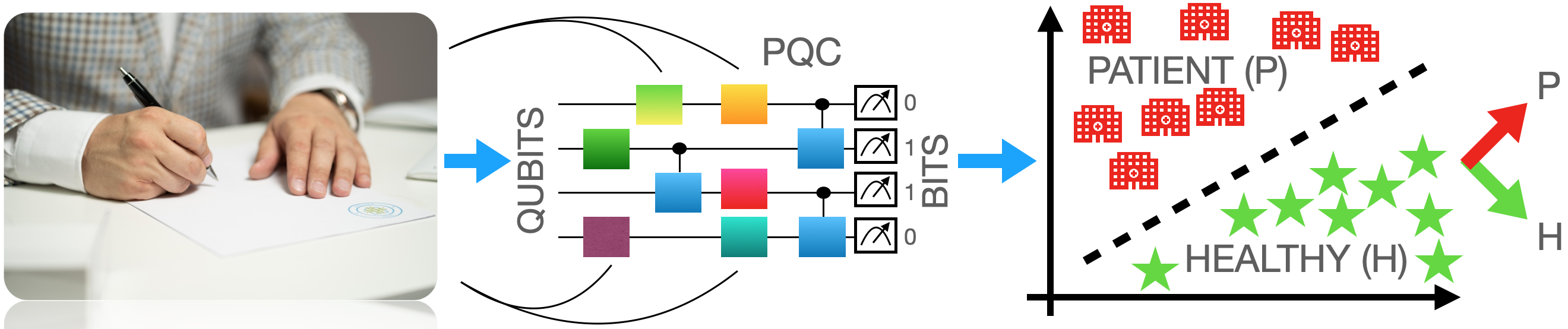
Figure 1: The data obtained from the handwriting tasks are processed and mapped into quantum states through a parametrized quantum circuit (PQC). Then a classification algorithm is applied to distinguish the samples between ‘patient’ (P) and ‘healthy’ (H).

1 Introduction

Neurodegenerative diseases are incurable conditions caused by the progressive degeneration of nerve cells [1]. Alzheimer’s disease (AD) is one of the most common amongst them [2]. The predominant symptom in the early phase of AD is episodic memory impairment followed by progressive amnesia, a result of widespread brain damage. Since there is no cure for AD, it is critical to improve the approaches now used for diagnosis [3]. Handwriting is a task that involves both cognitive and motor functions to plan and properly execute the movements that are required with high coordination [4]. The analysis of handwriting and drawing dynamics is a valid non-invasive way for evaluating AD progression. For this purpose a protocol of 25 tasks was defined in Ref. [5]. Each handwriting/drawing task is described by 18 features and the data collected amongst a group of healthy people and patients made up the DARWIN (Diagnosis AlzheimeR WIth haNdwriting) dataset. In Ref. [6] it is described how this dataset can be exploited by machine learning models to discriminate between AD patients and healthy people.

Machine learning (ML) is the field of artificial intelligence (AI) that studies the development of learning models to recognize, for example, patterns in large sets of data [7]. These models can learn how to attribute outputs to unseen inputs for classification or regression tasks (supervised learning), or find a structure in the inputs (unsupervised learning) for clustering or dimensionality reduction [8]. A lot of work has been done in the past years to improve the performance of ML algorithms and make them capable of handling efficiently big datasets. One more recent and promising solution could be to use quantum machine learning (QML) techniques. In QML inputs are encoded in quantum states and computation is done on a quantum computer [9, 10]. Although quantum processing units (QPUs) are still subjected to relatively large noise rates, it seems that applications in ML can lead to remarkable results. For example, in Ref. [11] it is shown how variational quantum models, namely models based on updating parameters in a quantum circuit through classical optimization, can exhibit a significant learning advantage in solving a regression task with input data from the fashion-MNIST dataset. A review of the contributions of QML in medical image analysis is given in Ref. [12]. A previous study [13] approaches via a so-called variational quantum classifier (VQC) the problem of classification defined by the same dataset we consider in our work.

Here we focus in particular on quantum kernel methods, i.e. kernel methods in which the feature space is a space of quantum states. We use these algorithms to classify the samples and compare their performances with the ones achieved by classical algorithms. The paper is organized as follows. In Section 2 we describe how the DARWIN dataset was created and we define the classical and quantum kernel methods for classification. Then in Section 3 and 4 we report their performances, we discuss the results and draw our conclusions.

2 Methods

2.1 Dataset

The DARWIN dataset is composed of handwriting data collected according to the protocol defined in Ref. [5]. It includes 25 tasks that can be divided in the following categories: graphic tasks, like joining points and drawing geometrical figures; copy tasks, testing the ability of repeating more complex gestures to write letters, numbers and words; memory tasks, involving writing previously memorized words; and dictation tasks. The protocol was submitted to 174 participants: 89 AD patients and 85 healthy people, recruited so that the two groups would match in terms of age, education and gender. None of the participants was taking medications that influenced their cognitive abilities. The tasks were performed on paper sheets put on top of a tablet equipped with a pen that could both write in ink and sample coordinates of the tip and pressure exerted. The tablet was connected to a PC that recorded movements and displayed them in real-time. A software was used to extract 18 features for each task. Features and tasks are described in details in Appendix A. The dataset includes also a feature for identification of participants and another one that indicates whether the sample is associated to an AD patient (P) or an healthy person (H). This feature is used as label in the classification problem via a (classical or quantum) supervised learning model.

2.2 Support vector classification (SVC)

2.2.1 Classical SVC

Support vector machines (SVMs) are indeed supervised learning models for classification and regression [14]. Considering a binary classification problem in which the aim is to decide whether a set of samples belongs to one of two classes, each data point is viewed as a $d$-dimensional vector. The goal is to separate the points with a $(d-1)$-dimensional hyperplane such that the distance from the hyperplane to the nearest data points on each side, called support vectors, is maximized. A graphic representation of this is given in Fig. 2. In the original space this problem has often no solution, i.e. the sets of point are not linearly separable. A SVM uses the kernel trick, the technique of mapping inputs into high-dimensional feature spaces, to solve this problem [15]. The dot products of input pairs in the feature space are called kernels. Defining a map $\varphi:\mathcal{X}\rightarrow\mathcal{F}$ from the original input space to the feature space is equivalent to defining a kernel function $k:\mathcal{X}\times\mathcal{X}\rightarrow\mathbb{C}$ that maps couples of inputs into their dot products in the feature space.

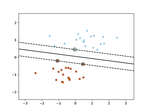
Figure 2: Graphic representation of a classification model in dimension $d=2$. The hyperplane is a straight line. Support vectors are circled.

For our classification task we consider 3 different kernel functions [16]. The radial basis function (RBF) kernel maps a pair of inputs $(x,x^{\prime})$ into $k_{rbf}(x,x^{\prime})=\exp\left(-\gamma|x-x^{\prime}|^{2}\right).$ This is one of the most common choices amongst kernel functions and it is used by default in the standard version of SVC implemented in the Scikit library in Python [17]. The linear kernel function is a simple dot product, $k_{lin}(x,x^{\prime})=\langle x,x^{\prime}\rangle.$ Lastly, the sigmoid kernel is given by $k_{sig}(x,x^{\prime})=\tanh(\gamma\langle x,x^{\prime}\rangle+r)$.

2.2.2 Quantum SVC

In the quantum version of SVMs, inputs are mapped into the space of quantum states [18]. The feature map is defined by a parametrized quantum circuit (PQC), whose parameters are given by the features of the inputs. A PQC is a sequence of parametrized unitary operators, called quantum logical gates, acting on a set of qubits, or quantum bits, which are two-state quantum systems [19]. To introduce the representation of qubit states, we need to define Dirac’s notation for unit vectors in $\mathbb{C}^{2}$. The standard basis of $\mathbb{C}^{2}$ is given by the vectors $\{|0\rangle,|1\rangle\},$ where $|0\rangle=\begin{pmatrix}1\\ 0\end{pmatrix}$, and $|1\rangle=\begin{pmatrix}0\\ 1\end{pmatrix}$. A generic unit vector in $\mathbb{C}^{2}$ is $|\phi\rangle=\alpha|0\rangle+\beta|1\rangle$, where $\alpha,\beta\in\mathbb{C}$ are such that $|\alpha|^{2}+|\beta|^{2}=1.$ The inner product of two unit vectors $|\phi\rangle,|\psi\rangle\in\mathbb{C}^{2}$ is denoted by $\langle\phi|\psi\rangle,$ while their outer product is $|\phi\rangle\langle\psi|.$ The state of a qubit is defined by a hermitian, positive semi-definite matrix $\rho\in\mathbb{C}^{2\times 2}$, such that its trace is equal to 1. The state is pure when there exists a $|\phi\rangle\in\mathbb{C}^{2}$ such that $\rho=|\phi\rangle\langle\phi|$, otherwise it is mixed.

To compute kernels we measure the fidelity of pairs of quantum states. Fidelity evaluates the degree of similarity of a pair of quantum states [20]. Given a pair of pure quantum states $\rho=|\phi\rangle\langle\phi|$ and $\sigma=|\psi\rangle\langle\psi|,$ their fidelity is defined by $\mathcal{F}(\rho,\sigma)=|\langle\phi|\psi\rangle|^{2}$. The most used generalization of this definition for a generic pair of mixed states $\rho$ and $\sigma$ is $\mathcal{F}(\rho,\sigma)=\left(\mathrm{tr}\sqrt{\sqrt{\rho}\sigma\sqrt{\rho}}\right)^{2}$. The calculation of fidelities is the only computation requiring a quantum hardware. All other computations in quantum SVCs are handled by a classical hardware.

Quantum SVC is implemented using the standard version in Scikit library with precomputed kernels. We use different PQCs, scaling the number of qubits with similar ansatze. The ansatze are chosen considering the following aspects. The number of quantum gates needs to be small enough to make the time needed to perform the calculations as small as possible. Time of execution is a critical point in quantum computation, since it is often limited on real QPUs. Given a kernel function $k$, the Gram matrix associated to it is the matrix whose entries are $G_{ij}=k(x_{i},x_{j}),$ where $x_{i}$ and $x_{j}$ are two inputs. The eigenvalue curve of the matrix $G$ is flat when the problem is difficult to learn, whereas a desirable situation is found when the eigenvalue curve is non-flat and decays, either polynomially or exponentially fast [21]. An ansatz is expressive when it explores the space of unitaries as fully and uniformally as possible. Expressive ansatze are desirable when facing a problem with no prior knowledge of it, because of their ability to adapt to the task. However it is proved that expressive anstatze are difficult to train [22], while an ansatz with low expressibility is easier to train and can achieve a better performance on the task it is specialized to solve [23]. One possible solution to reduce expressibility is introducing a bandwidth factor, a scaling hyperparameter that multiplies the parameters in the PQC. The bandwidth parameter limits the reach of the feature map [24].

The PQCs we use are composed of $R_{x}$ and $R_{y}$ rotation gates, coontrolled-z and controlled-x gates. The gates $R_{x}$ and $R_{y}$ are 1-qubit parametrized unitaries that perform a rotation of an angle given by its parameter about the x-axis and the y-axis of the Bloch sphere, respectively. The Bloch sphere is a 3-dimensional geometrical representation of the states of a qubit. The matrix representations of the rotation gates are the following:

$$R_{x}(\theta)=\begin{pmatrix}\cos\left(\frac{\theta}{2}\right)&-i\sin\left(\frac{\theta}{2}\right)\\ -i\sin\left(\frac{\theta}{2}\right)&\cos\left(\frac{\theta}{2}\right)\end{pmatrix},\quad R_{y}(\theta)=\begin{pmatrix}\cos\left(\frac{\theta}{2}\right)&-\sin\left(\frac{\theta}{2}\right)\\ \sin\left(\frac{\theta}{2}\right)&\cos\left(\frac{\theta}{2}\right)\end{pmatrix}.$$

A controlled gate is a quantum operation acting on multiple qubits. One or more qubits act as controls, i.e. based on their configuration, a certain gate is applied or not to the remaining qubit, called target. The controlled-x gate is a 2-qubits controlled gate. When the control is in the state $|1\rangle$ an $X$ gate is applied to the target, where $X=\begin{pmatrix}0&1\\ 1&0\end{pmatrix}.$ The controlled-z is also a 2-qubits controlled gate. It is symmetric, meaning that both qubits act as control, activated by the state $|1\rangle$, and target. The matrix representations of controlled-x and controlled-z gates are

$$CX=\begin{pmatrix}1&0&0&0\\ 0&1&0&0\\ 0&0&0&1\\ 0&0&1&0\end{pmatrix},\quad CZ=\begin{pmatrix}1&0&0&0\\ 0&1&0&0\\ 0&0&1&0\\ 0&0&0&-1\end{pmatrix}.$$

A control qubit activated by the state $|1\rangle$ is represented in a circuit as $\bullet.$ A target qubit to which an $X$ gate is applied is denoted by $\oplus$. Therefore the graphic representations of controlled-x and controlled-z in the circuits are, respectively, the following.

& 1 1

In Fig. 3 we show the graphic representation of our 6-qubits circuit, composed by layers of $R_{x}$ and $R_{y}$ gates alternating with layers of controlled-z and controlled-x gates. On the right-hand side are symbols representing measurements applied to the qubits, converting the quantum states in a sequence of classical bits. The number of circuit parameters is 24.

Figure 3: Graphic representation of the 6-qubits PQC that maps a sample $s=(s[0],s[1],...,s[23])$ into a quantum state. The parameters in the rotation gates are given by a bandwidth factor $b=0.4$, chosen in order to maximize mean accuracy, times the components of $s$.

A similar structure with the same number of parameters is used to define also an 8-qubits and a 12-qubits circuit. The number of parameters must be equal to the number of features of the samples, so that each input feature corresponds to a parameter. Therefore the dataset needs to be processed through a principal component analysis (PCA) prior to applying the methods [25]. In order to reduce expressibility, the parameters in the rotation gates are multiplied by a bandwidth hyperparameter, chosen so as to maximize the accuracy reached by the classification. These circuits produce kernel matrices whose eigenvalue curve are plotted in Fig. 4. The curves are not flat but decay, hence the problem can be solved in this way.

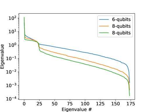
Figure 4: Plot (in logarithmic scale) of the eigenvalue curves associated with the kernel matrices defined by the 6-qubits, 8-qubits and 12-qubits circuit described in the main text.

2.3 Implementation

Our algorithms are implemented in Python, using the functionalities of Scikit and Qiskit libraries [26]. First we perform some preprocessing on the dataset. In particular we drop the identification feature, while keeping the feature healthy/AD’s patient (H/P) as a label. We standardize the samples, by subtracting the mean and scaling to unit variance. Then we perform a PCA with 24 components. Finally we standardize the set of samples derived from the PCA. In fact, from our analysis it emerges that this second normalization improves the performance of both classical and quantum methods. To reduce the bias introduced by selecting the samples for training and test, we select randomly 20 different splittings of the dataset in training and test set, keeping for the latter 21% of the samples, so that 137 samples are used for training and 37 for test. We use the same splittings for all methods.

After that we run classical SVCs using 3 different kernel functions: a radial basis function, a linear function and a sigmoid function. Subsequently we run the quantum SVCs for each of the 3 PQCs. Besides imposing the choice of the kernel function in the classical SVCs and the option of precomputing the kernels in the quantum SVCs, we keep the default setting for the other options of command ‘SVC’. For each run we compute the accuracy score, i.e. the number of test samples labelled correctly divided by the total number of test samples, and finally we calculate and compare the obtained average accuracies.

Table 1: Accuracy (in percentage) of classical SVCs and quantum SVCs for 20 different splittings of the dataset in training and test set. The highest accuracy in each run is reported in red.

Classical SVC			Quantum SVC
Rbf	Linear	Sigmoid	6 qubits	8 qubits	12 qubits
81.08	86.49	86.49	86.49	83.78	89.19
83.78	81.08	86.49	83.78	81.08	81.08
75.68	67.57	83.78	78.38	75.68	75.68
94.59	89.19	81.08	91.89	91.89	91.89
83.78	81.08	81.08	81.08	86.49	83.78
89.19	83.78	91.89	94.59	89.19	91.89
91.89	78.38	89.19	91.89	94.59	91.89
91.89	83.78	89.19	89.19	91.89	89.19
89.19	89.19	86.49	83.78	91.89	89.19
94.59	97.30	91.89	89.19	94.59	94.59
86.49	86.49	86.49	89.19	83.78	86.49
94.59	91.89	86.49	91.89	94.59	91.89
86.49	83.78	78.38	81.08	86.49	86.49
78.38	83.78	83.78	81.08	86.49	89.19
86.49	75.68	75.68	81.08	81.08	81.08
86.49	89.19	89.19	89.19	94.59	89.19
86.49	86.49	81.08	81.08	89.19	86.49
83.78	86.49	81.08	86.49	91.89	86.49
86.49	83.78	83.78	83.78	89.19	86.49
83.78	83.78	89.19	83.78	91.89	91.89

3 Results and Discussion

In Table 1 and in Fig. 5 we show the accuracy reached by the methods for each of the 20 splittings of the dataset in training and test set. Amongst classical SVCs, the one defined by the RBF kernel achieves average accuracy of 86.76%. Linear kernel and sigmoid kernel obtain 84.46% and 85.14% respectively. The quantum SVC defined by the 6-qubits PQC gets to 85.95%, the one defined by the 8-qubits PQC reaches 88.51% and the one defined by the 12-qubits circuit achieves average accuracy of 87.70%. One of the classical methods performs better than any other quantum method for 5 splittings. In 3 other splittings the same best precision is achieved by a classical and a quantum method. In the other 12 cases the quantum methods perform better. In particular, the 6-qubits method performs best in 2 splittings, the 8-qubits method in 7 splittings, the 12-qubits method achieves the best precision in 2 cases, while it obtains the same best accuracy of the 8-qubits method in 1 other case.

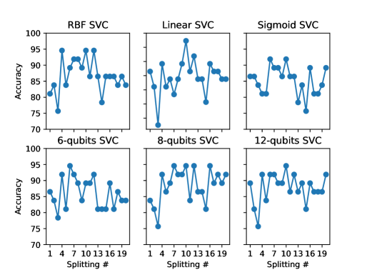
Figure 5: Accuracies (in percentage) vs. splittings of the dataset in classical and quantum SVC models.

3.1 Data subsampling

Now we repeat the analysis above when restricted to only one category of features, e.g. the features derived only from graphic tasks or only copy tasks or only memory and dictation tasks. We compare the performance of the classical and quantum SVCs that have achieved the highest average accuracies above, i.e. the classical SVC defined by the RBF kernel and the 8-qubits quantum SVC.

Table 2: Accuracies (in percentage) of RBF classical SVC and 8-qubits SVC achieved combining with the majority vote decision rule the predictions made considering all tasks individually (left) and considering only the best 5 tasks (right). The highest accuracy in each run is reported in red.

All tasks		Best 5 tasks
Classical	Quantum	Classical	Quantum
78.38	81.08	89.19	91.89
81.08	78.38	86.49	86.49
72.97	72.97	86.49	83.78
78.38	81.08	91.89	91.89
81.08	81.08	91.89	91.89
78.38	81.08	81.08	83.78
89.19	89.19	86.49	86.49
72.97	75.68	81.08	83.78
83.78	86.49	91.89	91.89
91.89	94.59	94.59	94.59
89.19	83.78	89.19	89.19
70.27	72.97	89.19	89.19
75.68	72.97	81.08	83.78
78.38	78.38	81.08	81.08
81.08	81.08	78.38	78.38
78.38	83.78	83.78	83.78
89.19	91.89	89.19	86.49
86.49	83.78	94.59	89.19
75.68	78.38	89.19	89.19
75.68	81.08	86.49	86.49

We use the same 20 splittings of the dataset in training and test set we have used above. First we take into account the features derived from the tasks in the category ‘graphic’. RBF and 8-qubits SVC achieve average accuracies of 79.19% and 79.86% respectively. After that we consider only the features derived from the tasks in the category ‘copy’. Both classical and quantum SVC achieve average accuracies of 83.11%. Finally, we focus on the features derived from the tasks in the category ‘memory and dictation’. Classical and quantum SVC achieve mean accuracies of 79.46% and 78.38%.

Subsequently we consider the features obtained from each of the 25 task individually. For each task we run RBF SVC, store the predictions made by the 25 models and use the majority vote decision rule [27] to select the outputs; namely for each sample we select the output predicted by most of the models. Likewise we run for each task a quantum SVC. Since each task is described by 18 features, we need to define a new PQC with 18 parameters. For this purpose we choose a 9-qubits circuit. No PCA is necessary in this case, since the number of parameters coincides with the number of features. We perform 20 runs with the same splittings in training and test set we have used above. The accuracies reached at each run are shown in Table 2. Classical and quantum SVC obtain mean accuracies of 80.41% and 81.49% respectively. Afterwards we select the best 5 tasks, namely the tasks that have achieved singularly the best accuracies in the previous runs. For both classical and quantum SVC the best tasks, although in a different order, are 23, 19, 17, 24 and 8. The tasks are described in Appendix A. As before we use the majority vote decision rule to select the predictions amongst those made by the 5 models associated with the tasks. In this case both classical and quantum SVC obtain average accuracies of 87.16%.

3.2 Noise robustness

Due to limited accessibility to real quantum hardware, computation of kernels is simulated without noise on a classical hardware, using tools from Qiskit library. To show how noise affects our results, we implement some models introducing depolarizing, bit-flip and amplitude damping errors [28].

First we consider the quantum SVC defined by the 6-qubits PQC. We select a splitting of the dataset in training and test set and we run the method without any noise. Then we add noise through the depolarizing error model, initially with error rate $p=0.01$, and after that we progressively increase $p$ by 0.01. For each run we compute the achieved accuracy. We repeat it also for bit-flip error and amplitude damping error, and subsequently we perform the same analysis for the 8-qubits and the 12-qubits methods. For the latter methods, excessive computational cost makes it necessary to reduce the number of samples before running the methods. In particular we consider 20 samples per label for the 8-qubits method, and 15 samples per label for the 12-qubits method.

In Fig. 6 we show how the accuracies of the 6-qubits SVC vary as the noise rate $p$ increases in the 3 different noise models. The accuracy curves stop at the $p$ value where the methods collapse, namely at $p^{*}$ such that for all $p\in[p^{*},1]$ the accuracy is the same as the one obtained at $p^{*}$. In the 8-qubits and 12-qubits SVCs, since the amount of noise injected grows with the number of qubits, the collapse happens for smaller $p^{*}$. All methods seems to be more robust to amplitude damping error than to depolarizing and bit-flip errors.

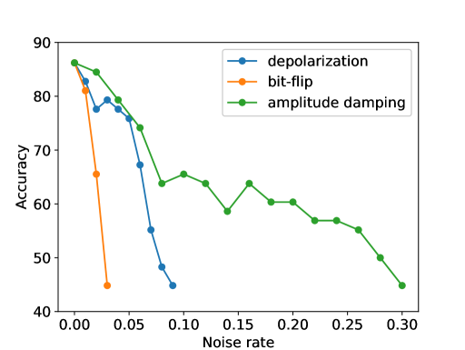
Figure 6: Accuracies (in percentage) of 6-qubits SVC as noise rate increases in the depolarizing, bit-flip and amplitude damping noise models.

4 Conclusion

The aim of this work is comparing the performances of classical and quantum kernel methods for classifying samples of AD patients and healthy people subjected to handwriting tests. To achieve this, we have used first some classical approaches and then we have compared their performances with the ones achieved by quantum methods defined by various PQCs. Amongst classical SVCs, the one defined by the radial basis function kernel achieves average accuracy of 86.76%, while linear kernel and sigmoid kernel obtain 84.46% and 85.14% respectively. The quantum SVC defined by the 6-qubits PQC gets to 85.95%, the one defined by the 8-qubits PQC reaches 88.51% and the one defined by the 12-qubits circuit achieves average accuracy of 87.70%. The fact that the latter does not outperform the model defined by the 8-qubits circuit seems to indicate that performance does not automatically improve by increasing the number of qubits, and some ansatze are better suited for smaller PQCs, hence more feasible with the currently available quantum processors.

In addition to running the methods considering all features together we have also defined methods based on data subsampling. We have considered separately the features associated with the 3 categories of tasks, namely features derived from graphic tasks, copy tasks or memory and dictation tasks. With graphic features, RBF and 8-qubits SVC achieve average accuracies of 79.19% and 79.86% respectively. When considering copy features, both RBF and 8-qubits SVC achieve average accuracy of 83.11%. Using the features derived from the tasks in the category ‘memory and dictation’, RBF and 8-qubits SVC achieve average accuracies of 73.65% and 71.89% respectively. Then we have examined the features obtained from each of the 25 task individually, defining a model for each task, and we have used the majority vote decision rule to combine the predictions made by the 25 models. Classical and quantum SVC obtain mean accuracies of 80.41% and 81.49% respectively. When restricted to only the best 5 tasks, i.e. the tasks that have achieved singularly the best accuracies in the previous runs, both classical and quantum SVC obtain average accuracies of 87.16%.

Kernels in quantum methods have been calculated simulating quantum computation without noise. We have also investigated how different types of noise affect the performance of quantum methods. From our analysis it appears that the methods show good robustness to the error introduced by amplitude damping, which is associated to energy dissipation. In fact, quantum SVCs tend to perform poorly only for high value of the noise rate related to the damping probability. Both depolarization and bit flip error instead cause the methods to perform worse for smaller values of noise rate. However, on real quantum computers different sources of noise act simultaneously, due to interaction with the environment and interaction between qubits, or imperfect application of quantum gates [29]. Therefore quantum noise models, without in-depth physical experiments, can only partially tackle the complexity of this problem.

Our study shows that quantum methods can achieve better performances in classification tasks even involving big datasets, as for the case of medical data analysis. Nowadays only QPUs with a limited number of noisy qubits are available. However this does not seem to affect too much the capability of quantum kernel methods. Moreover the constant improvement of quantum technologies suggests that there is a lot of room for enhancements to make quantum methods achieve even better results.

The techniques used in our work may have a wide range of applications in QML algorithms for classification and regression, and can be implemented to enhance classical ML models for similar problems of early screening, e.g. detection of autism in children [30], or identification of various types of cancer [31, 32].

Data availability

The DARWIN dataset is available at https://archive.ics.uci.edu/dataset/732/darwin.

Code availability

The code used is available at request.

Appendix A Dataset details

The 25 handwriting/drawing tasks can be grouped in 3 categories: memory and dictation, graphic, copy. The tasks are described in Table 3.

Table 3: List of tasks performed. The tasks are divided in the categories memory and dictation (M), graphic (G), and copy (C).

#	Description	Category
1	Signature drawing	M
2	Join two points with a horizontal line, continuously for four times	G
3	Join two points with a vertical line, continuously for four times	G
4	Retrace a circle (6 cm of diameter) continuously for four times	G
5	Retrace a circle (3 cm of diameter) continuously for four times	G
6	Copy the letters ‘l’, ‘m’ and ‘p’	C
7	Copy the letters on the adjacent rows	C
8	Write cursively a sequence of four lowercase letter ‘l’, in a single smooth movement	C
9	Write cursively a sequence of four lowercase cursive bigram ‘le’, in a single smooth movement	C
10	Copy the word “sheet”	C
11	Copy the word “sheet” above a line	C
12	Copy the word “mum”	C
13	Copy the word “mum” above a line	C
14	Memorize the words “telephone”, “dog”, and “shop” and rewrite them	M
15	Copy in reverse the word “bottle”	C
16	Copy in reverse the word “house”	C
17	Copy six words (regular, non regular, non words) in the appropriate boxes	C
18	Write the name of the object shown in a picture (a chair)	M
19	Copy the fields of a postal order	C
20	Write a simple sentence under dictation	M
21	Retrace a complex form	G
22	Copy a telephone number	C
23	Write a telephone number under dictation	M
24	Draw a clock, with all hours and put hands at 11:05 (Clock Drawing Test)	G
25	Copy a paragraph	C

Each task is performed on a different paper sheet and the pile of 25 sheets is put on top of a Wacom’s Bamboo tablet equipped with a pen that can both write in ink on paper and allow the tablet to sample x-y coordinate on paper and on air within a maximum distance of 3cm. The tablet is connected to a PC that processes the raw data to obtain for each task the following features:

1. Total Time (TT): Total time spent to perform the entire task.

2. Air Time (AT): Time spent to perform in-air movements.

3. Paper Time (PT): Time spent to perform on-paper movements.

4. Mean Speed on-paper (MSP): Average speed of on-paper movements.

5. Mean Speed in-air (MSA): Average speed of in-air movements.

6. Mean Acceleration on-paper (MAP): Average acceleration of on-paper movements.

7. Mean Acceleration in-air (MAA): Average acceleration of in-air movements.

8. Mean Jerk on-paper (MJP): Average jerk of on-paper movements. Jerk is the variation of acceleration with respect to time.

9. Mean Jerk in-air (MJA): Average jerk of in-air movements.

10. Pressure Mean (PM): Average of the pressure levels exerted by the pen tip.

11. Pressure Var (PV): Variance of the pressure levels exerted by the pen tip.

12. GMRT on-paper (GMRTP): Generalization of the Mean Relative Tremor (MRT) as defined by Pereira et al. (2015). MRT measures the amount of tremor in drawing spirals and meanders.

13. GMRT in-air (GMRTA): Generalization of the Mean Relative Tremor computed on in air movements.

14. Mean GMRT (GMRT): Average of GMRTP and GMRTA.

15. Pendowns Number (PWN): Counts the total number of pendowns recorded during the execution of the entire task.

16. Max X Extension (XE): Maximum extension recorded along the X axis.

17. Max Y Extension (YE): Maximum extension recorded along the Y axis.

18. Dispersion Index (DI): The Dispersion Index measures how the handwritten trace is “dispersed” on the entire piece of paper. To calculate the index the sheet is ideally divided into TB boxes of 3 × 3 pixels, then the number CB of boxes containing a fragment of handwriting/drawing is computed. DI is given by the ratio between CB and TB.

References

- \bibcommenthead
- Dugger and Dickson [2017] Dugger, B.N., Dickson, D.W.: Pathology of neurodegenerative diseases. Cold Spring Harbor perspectives in biology 9(7), 028035 (2017) https://doi.org/10.1101/cshperspect.a028035
- Honig and Mayeux [2001] Honig, L.S., Mayeux, R.: Natural history of alzheimer’s disease. Aging Clinical and Experimental Research 13(3), 171–182 (2001) https://doi.org/10.1007/BF03351476
- Jellinger [1998] Jellinger, K.: The neuropathological diagnosis of alzheimer disease. Ageing and Dementia, 97–118 (1998) https://doi.org/10.1007/978-3-7091-6467-9_9
- Dooijes [1983] Dooijes, E.H.: Analysis of handwriting movements. Acta Psychologica 54(1-3), 99–114 (1983) https://doi.org/10.1016/0001-6918(83)90026-4
- Cilia et al. [2018] Cilia, N.D., Stefano, C.D., Fontanella, F., Di Freca, A.S.: An experimental protocol to support cognitive impairment diagnosis by using handwriting analysis. Procedia Computer Science 141, 466–471 (2018) https://doi.org/10.1016/j.procs.2018.10.141 . The 9th International Conference on Emerging Ubiquitous Systems and Pervasive Networks (EUSPN-2018) / The 8th International Conference on Current and Future Trends of Information and Communication Technologies in Healthcare (ICTH-2018) / Affiliated Workshops
- Cilia et al. [2022] Cilia, N.D., De Gregorio, G., De Stefano, C., Fontanella, F., Marcelli, A., Parziale, A.: Diagnosing alzheimer’s disease from on-line handwriting: A novel dataset and performance benchmarking. Engineering Applications of Artificial Intelligence 111, 104822 (2022) https://doi.org/10.1016/j.engappai.2022.104822
- Helm et al. [2020] Helm, J.M., Swiergosz, A.M., Haeberle, H.S., Karnuta, J.M., Schaffer, J.L., Krebs, V.E., Spitzer, A.I., Ramkumar, P.N.: Machine learning and artificial intelligence: Definitions, applications, and future directions. Current Reviews in Musculoskeletal Medicine 13, 69–76 (2020) https://doi.org/%****␣sn-article.bbl␣Line␣150␣****10.1007/s12178-020-09600-8
- Love [2002] Love, B.C.: Comparing supervised and unsupervised category learning. Psychonomic Bulletin & Review 9(4), 829–835 (2002) https://doi.org/10.3758/BF03196342
- Schuld et al. [2015] Schuld, M., Sinayskiy, I., Petruccione, F.: An introduction to quantum machine learning. Contemporary Physics 56(2), 172–185 (2015) https://doi.org/10.1080/00107514.2014.964942
- Schuld and Petruccione [2021] Schuld, M., Petruccione, F.: Machine Learning with Quantum Computers, 2nd edn. Quantum Science and Technology, p. 312. Springer, 978-3-030-83097-7 (2021). https://doi.org/10.1007/978-3-030-83098-4
- Jerbi et al. [2023] Jerbi, S., Fiderer, L.J., Poulsen Nautrup, H., Kübler, J.M., Briegel, H.J., Dunjko, V.: Quantum machine learning beyond kernel methods. Nature Communications 14(1), 517 (2023) https://doi.org/10.1038/s41467-023-36159-y
- Wei et al. [2023] Wei, L., Liu, H., Xu, J., Shi, L., Shan, Z., Zhao, B., Gao, Y.: Quantum machine learning in medical image analysis: A survey. Neurocomputing 525, 42–53 (2023) https://doi.org/10.1016/j.neucom.2023.01.049
- Akpinar [2023] Akpinar, E.: Quantum machine learning in the cognitive domain: Alzheimer’s disease study. arXiv preprint arXiv:2401.06697 (2023) https://doi.org/10.48550/arXiv.2401.06697
- Jakkula [2006] Jakkula, V.: Tutorial on support vector machine (svm). School of EECS, Washington State University 37(2.5), 3 (2006)
- Hofmann et al. [2008] Hofmann, T., Schölkopf, B., Smola, A.J.: Kernel methods in machine learning. The Annals of Statistics 36(3), 1171–1220 (2008) https://doi.org/10.1214/009053607000000677
- Kavzoglu and Colkesen [2009] Kavzoglu, T., Colkesen, I.: A kernel functions analysis for support vector machines for land cover classification. International Journal of Applied Earth Observation and Geoinformation 11(5), 352–359 (2009) https://doi.org/10.1016/j.jag.2009.06.002
- Pedregosa et al. [2011] Pedregosa, F., Varoquaux, G., Gramfort, A., Michel, V., Thirion, B., Grisel, O., Blondel, M., Prettenhofer, P., Weiss, R., Dubourg, V., Vanderplas, J., Passos, A., Cournapeau, D., Brucher, M., Perrot, M., Duchesnay, E.: Scikit-learn: Machine learning in Python. Journal of Machine Learning Research 12, 2825–2830 (2011) https://doi.org/10.48550/arXiv.1201.0490
- Schuld [2021] Schuld, M.: Supervised quantum machine learning models are kernel methods. arXiv preprint arXiv:2101.11020 (2021) https://doi.org/10.48550/arXiv.2101.11020
- Nielsen and Chuang [2010] Nielsen, M.A., Chuang, I.L.: Quantum Computation and Quantum Information: 10th Anniversary Edition. Cambridge University Press, 9781107002173 (2010). https://doi.org/10.1017/CBO9780511976667
- Liang et al. [2019] Liang, Y.-C., Yeh, Y.-H., Mendonça, P.E., Teh, R.Y., Reid, M.D., Drummond, P.D.: Quantum fidelity measures for mixed states. Reports on Progress in Physics 82(7), 076001 (2019) https://doi.org/10.1088/1361-6633/ab1ca4
- Goel and Klivans [2017] Goel, S., Klivans, A.: Eigenvalue decay implies polynomial-time learnability for neural networks. Advances in Neural Information Processing Systems 30 (2017) https://doi.org/10.48550/arXiv.1708.03708
- Holmes et al. [2022] Holmes, Z., Sharma, K., Cerezo, M., Coles, P.J.: Connecting ansatz expressibility to gradient magnitudes and barren plateaus. PRX Quantum 3(1), 010313 (2022) https://doi.org/10.1103/PRXQuantum.3.010313
- Kübler et al. [2021] Kübler, J., Buchholz, S., Schölkopf, B.: The inductive bias of quantum kernels. Advances in Neural Information Processing Systems 34, 12661–12673 (2021) https://doi.org/10.48550/arXiv.2106.03747
- Canatar et al. [2022] Canatar, A., Peters, E., Pehlevan, C., Wild, S.M., Shaydulin, R.: Bandwidth enables generalization in quantum kernel models. arXiv preprint arXiv:2206.06686 (2022) https://doi.org/10.48550/arXiv.2206.06686
- Howley et al. [2005] Howley, T., Madden, M.G., O’Connell, M.-L., Ryder, A.G.: The effect of principal component analysis on machine learning accuracy with high dimensional spectral data. In: International Conference on Innovative Techniques and Applications of Artificial Intelligence, pp. 209–222 (2005). https://doi.org/10.1007/1-84628-224-1_16 . Springer
- Qiskit contributors [2023] Qiskit contributors: Qiskit: An Open-source Framework for Quantum Computing (2023). https://doi.org/10.5281/zenodo.2573505
- Kittler et al. [1998] Kittler, J., Hatef, M., Duin, R.P., Matas, J.: On combining classifiers. IEEE transactions on pattern analysis and machine intelligence 20(3), 226–239 (1998) https://doi.org/10.1109/34.667881
- Caruso et al. [2014] Caruso, F., Giovannetti, V., Lupo, C., Mancini, S.: Quantum channels and memory effects. Reviews of Modern Physics 86(4), 1203 (2014) https://doi.org/10.1103/RevModPhys.86.1203
- Resch and Karpuzcu [2021] Resch, S., Karpuzcu, U.R.: Benchmarking quantum computers and the impact of quantum noise. ACM Computing Surveys (CSUR) 54(7), 1–35 (2021) https://doi.org/10.1145/3464420
- Abbas et al. [2018] Abbas, H., Garberson, F., Glover, E., Wall, D.P.: Machine learning approach for early detection of autism by combining questionnaire and home video screening. Journal of the American Medical Informatics Association 25(8), 1000–1007 (2018) https://doi.org/%****␣sn-article.bbl␣Line␣500␣****10.1093/jamia/ocy039
- Tahmooresi et al. [2018] Tahmooresi, M., Afshar, A., Rad, B.B., Nowshath, K., Bamiah, M.: Early detection of breast cancer using machine learning techniques (2018). https://jtec.utem.edu.my/jtec/article/view/4706
- Gould et al. [2021] Gould, M.K., Huang, B.Z., Tammemagi, M.C., Kinar, Y., Shiff, R.: Machine learning for early lung cancer identification using routine clinical and laboratory data. American Journal of Respiratory and Critical Care Medicine 204(4), 445–453 (2021) https://doi.org/10.1164/rccm.202007-2791OC
Acknowledgements
This work was supported by the European Commission’s Horizon Europe Framework Programme under the Research and Innovation Action GA n. 101070546–MUQUABIS, by the European Union’s Horizon 2020 research and innovation programme under FET-OPEN GA n. 828946–PATHOS, by the European Defence Agency under the project Q-LAMPS Contract No B PRJ- RT-989, and by the MUR Progetti di Ricerca di Rilevante Interesse Nazionale (PRIN) Bando 2022 - project n. 20227HSE83 – ThAI-MIA funded by the European Union - Next Generation EU.
G. C. is a member of INFM (INdAM).