F3low: Frame-to-Frame Coarse-grained Molecular Dynamics with SE(3) Guided Flow Matching
Abstract
Molecular dynamics (MD) is a crucial technique for simulating biological systems, enabling the exploration of their dynamic nature and fostering an understanding of their functions and properties. To address exploration inefficiency, emerging enhanced sampling approaches like coarse-graining (CG) and generative models have been employed. In this work, we propose a Frame-to-Frame generative model with guided Flow-matching (F3low) for enhanced sampling, which (a) extends the domain of CG modeling to the Riemannian manifold; (b) retreating CGMD simulations as autoregressively sampling guided by the former frame via flow-matching models; (c) targets the protein backbone, offering improved insights into secondary structure formation and intricate folding pathways. Compared to previous methods, F3low allows for broader exploration of conformational space. The ability to rapidly generate diverse conformations via force-free generative paradigm on paves the way toward efficient enhanced sampling methods.
1 Introduction
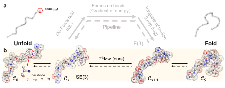
Molecular dynamics (MD) is a computational technique that simulates the motion and behavior of biological macromolecules systems without the need for wet lab experiments. By employing physics-based force fields and algorithms, MD provides valuable insights into the dynamic aspects of protein structures, such as protein folding event (Lindorff-Larsen et al. (2011), Fig. 1). This approach is instrumental in elucidating the functions and interactions of proteins at atomic level.
However, MD simulations faces challenges in efficiently exploring the conformation space due to the difficulty of crossing the high energy-barriers, which requires milliseconds of simulation steps and renders infeasible. To address this issue, enhanced sampling methods are developed to encourage the feasible exploration of conformation space via MD simulations. One of the enhanced sampling methods is coarse-grained molecular dynamics (CGMD) (Kmiecik et al. (2016)). It involves creating a coarse-grained representation by slicing out atoms from each residue up to its , termed as beads shown in Fig. 1(a). In this process, atomistic forces generated by potential functions or machine learning force fields are applied to beads on the CG space to perform simulations. This facilitates the smoothing of energy landscapes, preventing the occurrence of traps in local minima. Another emerging method utilizes probabilistic generative models to generate conformations targeting the Boltzmann distribution, without the dependency of empirical forces and motion integration (Fig. 1(b)). Klein et al. (2023) employs normalizing flow to map structures of small peptides from Gaussian noises for the next step, highlighting transferability between states with relatively larger timesteps.
In this paper, we leverage the advantages of both CGMD and generative models, presenting F3low, for enhanced sampling. Firstly, we extend the common modeling resolution of CGMD from level to backbone level (, Fig. 1(b)). In essence, the space of conformation poses is expanded from (or ) to , with denoting the number of residues. In such way, it preserves the structural geometry, enabling the direct observation of the secondary structure and folding pathway without the need for any reconstruction. Secondly, we leverage the guided flow on the SE(3) manifold (Lipman et al. (2022); Chen & Lipman (2023); Zheng et al. (2023)) to perform the simulation in a backbone-resolution. Concretely, as illustrated in Fig. 1(b), F3low samples the next frame from prior distribution (e.g., zero center of mass Gaussian) while being guided by the preceding frame at step . We term this sampling based on conditional probability as frame-to-frame simulation. This process can be repeated for steps to conduct complete simulations. Compared with Klein et al. (2023), F3low is not confined to small peptides (under 4AA) but can handle larger fast folding proteins (Lindorff-Larsen et al. (2011)) spanning from Chignolin (10AA) to Homeodomain (54AA) benefiting from the advantage of coarse-graining.
2 Methods
Given a conformation frame at step , we leverage a probabilistic generative model to sample the next frame guided by from a prior source distribution :
| (1) |
This iterative process, starting from an initial frame and repeated times, results in the generation of a complete trajectory . We refer to this procedure based on conditional probability as frame-to-frame simulation illustrated in Fig. 1(b). After the simulations, we can conduct various trajectory analysis of protein dynamics, including comparing free energy surfaces and calculating transition probabilities between meta-stable states.
2.1 SE(3) guided flow matching
In this context, we provide a brief introduction to the general concept of Riemannian flow matching, followed by its extension to the SE(3) space. Then we introduce the basic concept of guided flow.
From Riemannian to SE(3) flow matching. We consider complete connected, smooth Riemannian manifolds endowed with metric . At each point can attach to a Tangent space and the metric is defined as inner product over . The continuous normalizing flow (CNF) is defined as the solution of the following ordinary differential equation (ODE) along with a time-dependent vector field : , with initial conditions . Density distribution on Riemannian manifolds is continuous non-negative functions the integrate to . Given two distributions and on , we can define a probability path as their interpolation. In other word, is a sequence of probability distributions generated by vector field through pushing forward to . To learn a CNF, flow-matching (FM) is proposed (Albergo & Vanden-Eijnden (2022); Lipman et al. (2022)) as a simulation-free method by regressing vector field with a parametric one . Since computing is intractable and cannot be directly targeted, we always adopt conditional flow matching (CFM), attaching with a conditional probability path satisfying and . is the delta probability concentrating all its mass at . Subsequently, the unconditional can be recovered by calculating marginal distribution . The objective of training CFM is to minimize with conditional vector field . When plugging the conditional flow with initial condition into the CFM loss, we can reparameterize with , and rewrite the final CFM loss as:
| (2) |
where , and is the norm induced by Riemannian metric .
The basic structure of protein backbone is characterized by a rigid transformation (Jumper et al. (2021)), where this transformation can be decomposed into a rotation and translation vector . Following Yim et al. (2023b; a), the metric on is where is the vector in tangent space of , referring to , and denotes the trace of the matrix. The metric on is where . Combining these two metrics, we derive the metric on as . It allows us construct the conditional flow connecting source distribution and target distribution . Given and , is denoted as the geodesic interpolant path represented on and respectively:
| (3) | ||||
where is logarithm map converting elements in to , and is exponential map for inverting the logarithm map. Referring to Yim et al. (2023a), the objective can be written as directly predicting the target:
| (4) |
where and are the prediction of .
Guided flow. Guided flow is first introduced by Zheng et al. (2023), which is an adaptation of classifier-free guidance Ho & Salimans (2022) to FM models for conditional generation. Given the condition , we can extend the unconditional to and corresponding vector field . Following Zheng et al. (2023), the guided vector field can be derived from the combination of :
| (5) |
where is a manually selected weight. Zheng et al. (2023) also showcases that is related to score function by , with and as schedulers 111Zheng et al. (2023) only showcases the guided flow on . We will add the proof of its generalization on in the future work..
2.2 F3low for coarse-grained molecular dynamics
In this part, we introduce our methods, F3low, which provides a new perspective on coarse-grained molecular dynamics by iteratively generating conformation frames in a trajectory using a guided flow-matching model. We outline the basic concept, elaborate on integrating conformation guidance into the flow-matching models based on initial guesses, and provide an overview of the training and sampling procedures.
Basic concept. As defined in Eq. 1, we leverage a trained guided flow-matching model to sample the next frame. To be consistent with the aforementioned definitions, we denote , and . The conformation is modeled with coarse-graining at the protein backbone level, consisting of 4 heavy atoms . Let denote the number of residue within , the space of conformation poses is , where each residue is mapped by a rigid transformation with . And hence . To preserve the symmetries, all the translations are carried out within the zero center of mass (CoM) subspace. This ensures that the prior source distribution and the intermediate remain -invariant, and the vector field maintains -equivariance. Here we denote the prior distribution in Eq. 1 as where represents the Gaussian distribution on subtracted the CoM. Following Yim et al. (2023a); Watson et al. (2023), serves as the isotropic Gaussian distribution .
It is noteworthy that we cannot directly define a flow from to since they belong to the same trajectory and, therefore, are under the same Boltzmann distribution, rather than two separate distributions. Instead, we formulate the problem as a guided flow, where we sample guided by from a normal prior distribution. This aligns with the definition of flow in this context.
Integration of conformation guidance. As demonstrated in Eq. 3, and represent the linear interpolation of and . Then these values are utilized as the input for , which predicts the target and . In the context of classifier-free guidance, incorporating the condition (the former conformation ) into the FM model poses challenges in the case of protein structures. Unlike image or text labels, representing 3D protein structures is non-trivial. Various attempts have been proposed, including methods such as template embedding (Jumper et al. (2021)) or treating the structures as initial guesses before recycling (Bennett et al. (2023)). Motivated by Bennett et al. (2023), we also consider as a form of initial guess, and integrate it into as a weighted average in space:
| (6) | ||||
where is a hyperparameter termed as initial guess weight. During training, it is necessary to compute the optimal transport (OT) between and . And hence the derivation of can be re-written:
| (7) |
Then we subtract the CoM of to ensure equivariance. Such linear interpolation helps better preserve the structure information while keeping the model architecture unchanged. Detailed training and sampling procedures are provided in Appendix Algorithm 1 and Algorithm 2.
3 Experiment
3.1 Free Energy Surface
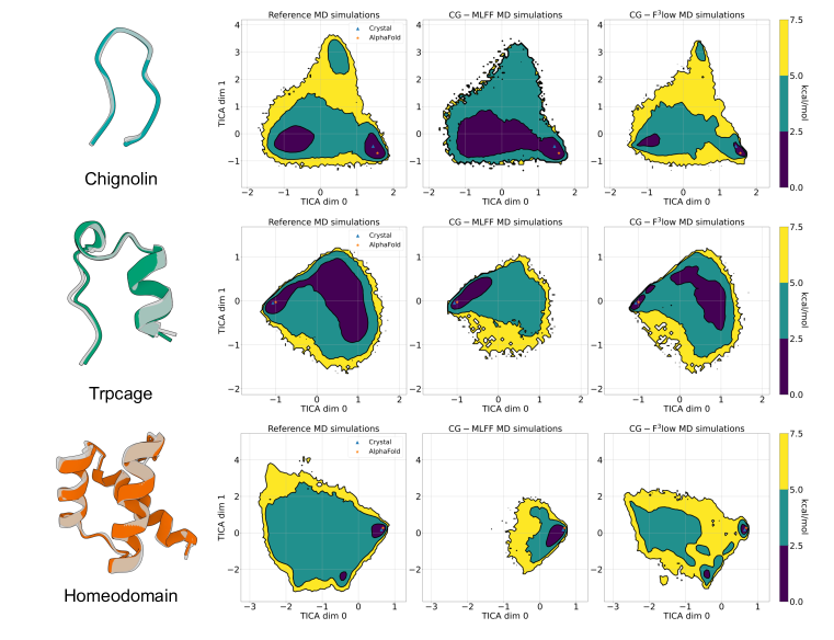
To validate the capabilities of the F3low model for conformational space exploration, we conducted training and sampling procedures (see details on Appendix D) on three representative fast-folding proteins: Chignolin, a -hairpin structure; Trpcage, dominated by its dominant -helix; and Homeodomain, a complex assembly of three helices. Further comparative analysis with the coarse-grained machine learning force field (CG-MLFF) simulations (Majewski et al. (2023)), which focus solely on the atom, has demonstrated the superior performance of our approach in accurately depicting secondary structures by considering all backbone atoms.
| Reference | CG-MLFF | CG-F3low | ||
|---|---|---|---|---|
| Chignolin | 0.15 | 0.17 | 0.14 | |
| Backbone | 0.27 | 0.89 | 0.36 | |
| Trpcage | 0.45 | 1.03 | 0.56 | |
| Backbone | 0.58 | 2.41 | 0.62 | |
| Homeodomain | 0.56 | 2.17 | 0.51 | |
| Backbone | 0.54 | 2.11 | 0.53 |
For the purpose of dimensionality reduction, we applied time-lagged independent component analysis (Pérez-Hernández et al. (2013), TICA) to both the CG-MLFF and CG-F3low simulation trajectories. This analysis projected the data onto the leading three or four components, utilizing covariance matrices derived from the reference MD simulations. Additionally, we constructed Markov state models (Husic & Pande (2018), MSMs) and applied a reweighting technique to the free energy surfaces, leveraging the stationary distribution of the MSMs. Comprehensive details regarding the TICA and MSM parameters for each protein are provided in the Appendix B.
As illustrated in Fig. 2, our evaluation of two relatively simple proteins, Chignolin and Trpcage, demonstrates that both models achieve commendable coverage of the free energy surface. Notably, F3low presented a more precise energy distribution in comparison to the reference data. In the case of the larger protein, Homeodomain, we observed that the CG-MLFF simulations rapidly converged to the native structure and did not sufficiently sample the unstructured conformations. In contrast, F3low effectively explored these less-defined regions, achieving this with a reduced number of starting points (8 as opposed to 32). A broader exploration of the conformational space allows us to go even further in our in-depth analysis of Homeodomain, see Appendix C for more details.
Furthermore, we have superimposed the crystal structure and the AlphaFold-predicted (Jumper et al. (2021)) structure onto the free energy surface plots. The AlphaFold predictions align remarkably well with the actual crystal structure. Nevertheless, it represents a singular structure. The generative models, on the other hand, are capable of exploring a vastly expanded conformational space, thereby offering more profound insights into the dynamic behavior of proteins.
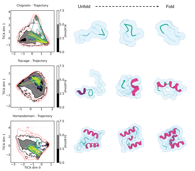
We also visualize an individual simulation trajectory for each protein in Fig. 3. The frames from diluted trajectories imply that our approach is capable of exploring a broader space of potential energy surfaces within a single trajectory, as opposed to solely depending on trajectory ensemble.
3.2 Comparison of simulated and crystal structures.
All simulations successfully identified the location of the global minimum on the free energy surface across all proteins. Subsequently, we conducted a comparative analysis of the minimum root-mean-square deviation (RMSD) values relative to the crystal structures, as detailed in Table 1. Our CG-F3low simulations consistently sampled structures with lower RMSD values than CG-MLFF simulations and showed comparable RMSD to the reference simulations. The efficacy of our algorithm is particularly pronounced when comparing in terms of the backbone. In contrast, CG-MLFF simulations require additional steps to reconstruct the backbone, highlighting the inherent advantages of our approach.
4 Conclusion
In this work, we present a novel enhanced sampling method named F3low, which is a frame-to-frame generative model with guided flow matching on . F3low extends the modeling domain to with a backbone level-resolution, providing improved insights into secondary structure information and intricate folding pathways. By analyzing the simulation trajectories of 3 representative proteins and comparing with traditional MLFF, we illustrate the F3low’s capacity for broadly exploring conformational spaces within a generative paradigm. In our future work, we intend to incorporate the physical analysis of the simulation trajectories, and conduct the remaining fast folding proteins. Additionally, the flow process on side-chain torsion angles would be included to perform all-atom protein molecule dynamics.
Acknowledgement
We thank the reviewers of GEM workshop for their valuable comments. We thank Adrià Pérez, the author of Majewski et al. (2023) for providing the detailed settings of free energy surface. We thank Le Zhuo for valuable discussions of flow matching methods.
This paper is supported by National Key Research and Development Program of China (2023YFF1205103), National Natural Science Foundation of China (81925034) and National Natural Science Foundation of China (62088102). This paper is also supported by the Natural Sciences and Engineering Research Council (NSERC) Discovery Grant, the Canada CIFAR AI Chair Program, collaboration grants between Microsoft Research and Mila, Samsung Electronics Co., Ltd., Amazon Faculty Research Award, Tencent AI Lab Rhino-Bird Gift Fund, a NRC Collaborative R&D Project (AI4D-CORE-06) as well as the IVADO Fundamental Research Project grant PRF-2019-3583139727.
References
- Albergo & Vanden-Eijnden (2022) Michael S Albergo and Eric Vanden-Eijnden. Building normalizing flows with stochastic interpolants. arXiv preprint arXiv:2209.15571, 2022.
- Bennett et al. (2023) Nathaniel R Bennett, Brian Coventry, Inna Goreshnik, Buwei Huang, Aza Allen, Dionne Vafeados, Ying Po Peng, Justas Dauparas, Minkyung Baek, Lance Stewart, et al. Improving de novo protein binder design with deep learning. Nature Communications, 14(1):2625, 2023.
- Chen & Lipman (2023) Ricky TQ Chen and Yaron Lipman. Riemannian flow matching on general geometries. arXiv preprint arXiv:2302.03660, 2023.
- DeMarco et al. (2004) Mari L DeMarco, Darwin OV Alonso, and Valerie Daggett. Diffusing and colliding: the atomic level folding/unfolding pathway of a small helical protein. Journal of molecular biology, 341(4):1109–1124, 2004.
- Ho & Salimans (2022) Jonathan Ho and Tim Salimans. Classifier-free diffusion guidance. arXiv preprint arXiv:2207.12598, 2022.
- Husic & Pande (2018) Brooke E Husic and Vijay S Pande. Markov state models: From an art to a science. Journal of the American Chemical Society, 140(7):2386–2396, 2018.
- Jumper et al. (2021) John Jumper, Richard Evans, Alexander Pritzel, Tim Green, Michael Figurnov, Olaf Ronneberger, Kathryn Tunyasuvunakool, Russ Bates, Augustin Žídek, Anna Potapenko, et al. Highly accurate protein structure prediction with alphafold. Nature, 596(7873):583–589, 2021.
- Klein et al. (2023) Leon Klein, Andrew YK Foong, Tor Erlend Fjelde, Bruno Mlodozeniec, Marc Brockschmidt, Sebastian Nowozin, Frank Noé, and Ryota Tomioka. Timewarp: Transferable acceleration of molecular dynamics by learning time-coarsened dynamics. arXiv preprint arXiv:2302.01170, 2023.
- Kmiecik et al. (2016) Sebastian Kmiecik, Dominik Gront, Michal Kolinski, Lukasz Wieteska, Aleksandra Elzbieta Dawid, and Andrzej Kolinski. Coarse-grained protein models and their applications. Chemical reviews, 116(14):7898–7936, 2016.
- Lindorff-Larsen et al. (2011) Kresten Lindorff-Larsen, Stefano Piana, Ron O Dror, and David E Shaw. How fast-folding proteins fold. Science, 334(6055):517–520, 2011.
- Lipman et al. (2022) Yaron Lipman, Ricky TQ Chen, Heli Ben-Hamu, Maximilian Nickel, and Matt Le. Flow matching for generative modeling. arXiv preprint arXiv:2210.02747, 2022.
- Majewski et al. (2023) Maciej Majewski, Adrià Pérez, Philipp Thölke, Stefan Doerr, Nicholas E Charron, Toni Giorgino, Brooke E Husic, Cecilia Clementi, Frank Noé, and Gianni De Fabritiis. Machine learning coarse-grained potentials of protein thermodynamics. Nature Communications, 14(1):5739, 2023.
- Mayor et al. (2000) Ugo Mayor, Christopher M Johnson, Valerie Daggett, and Alan R Fersht. Protein folding and unfolding in microseconds to nanoseconds by experiment and simulation. Proceedings of the National Academy of Sciences, 97(25):13518–13522, 2000.
- Pérez-Hernández et al. (2013) Guillermo Pérez-Hernández, Fabian Paul, Toni Giorgino, Gianni De Fabritiis, and Frank Noé. Identification of slow molecular order parameters for markov model construction. The Journal of chemical physics, 139(1), 2013.
- Watson et al. (2023) Joseph L Watson, David Juergens, Nathaniel R Bennett, Brian L Trippe, Jason Yim, Helen E Eisenach, Woody Ahern, Andrew J Borst, Robert J Ragotte, Lukas F Milles, et al. De novo design of protein structure and function with rfdiffusion. Nature, 620(7976):1089–1100, 2023.
- Yim et al. (2023a) Jason Yim, Andrew Campbell, Andrew YK Foong, Michael Gastegger, José Jiménez-Luna, Sarah Lewis, Victor Garcia Satorras, Bastiaan S Veeling, Regina Barzilay, Tommi Jaakkola, et al. Fast protein backbone generation with se (3) flow matching. arXiv preprint arXiv:2310.05297, 2023a.
- Yim et al. (2023b) Jason Yim, Brian L Trippe, Valentin De Bortoli, Emile Mathieu, Arnaud Doucet, Regina Barzilay, and Tommi Jaakkola. Se (3) diffusion model with application to protein backbone generation. arXiv preprint arXiv:2302.02277, 2023b.
- Zheng et al. (2023) Qinqing Zheng, Matt Le, Neta Shaul, Yaron Lipman, Aditya Grover, and Ricky TQ Chen. Guided flows for generative modeling and decision making. arXiv preprint arXiv:2311.13443, 2023.
Appendix A Training and Sampling
We describe the precise training and simulation process in Algorithm 1 and 2 over distribution in . Different from Yim et al. (2023b), frame in this paper is the snapshot within a trajectory, rather than the spatial structure of the protein backbone. In the training process line 7, when combining the initial guess, an alignment for to is performed before adding it to the transported . This step is implemented to maintain training stability. In the simulation process, the notation (line 10) refers to the Euler method.
Appendix B Markov state model estimation
Markov state models (MSMs) were constructed for the reference MD simulations, as well as for the CG-MLFF and CG-F3low simulations. For the reference simulations, in line with the methodologies outlined in previous research Majewski et al. (2023), simulation data were transformed into pairwise distances (excluding the terminal five residues of Trpcage). TICA was then employed to reduce the dimensionality of the featurized data, capturing the first 4, 3, and 3 principal components for Chignolin, Trpcage, and Homeodomain, respectively. The resulting components were clustered using the K-means algorithm, and this discretized data was utilized for MSM estimation. The CG-MLFF and CG-F3low simulations underwent an identical process. However, for these simulations, covariance matrices derived from the reference MD simulations were used during the TICA projection to ensure a consistent basis for comparison of the first 3 or 4 components. This step was crucial for assessing how accurately the coarse-grained simulations reproduce the free energy surfaces of proteins. To enhance the interpretability of the MSMs, the PCCA algorithm was applied to consolidate the microstates into macrostates. The comparative free energy surfaces were generated by partitioning the first two TICA components into an grid and adjusting them through reweighting using the MSM stationary distribution. The detailed parameters are listed in the table below.
| TICA lag time (steps) | # of TICA projection components | # of K-means clusters | MSM lag time (ns) | # of MSM macrostates | ||
|---|---|---|---|---|---|---|
| Reference | Chignolin | 20 | 4 | 1200 | 20 | 3 |
| Trpcage | 100 | 3 | 500 | 10 | 2 | |
| Homeodomain | 100 | 3 | 600 | 10 | 3 | |
| CG-MLFF | Chignolin | / | 3 | 200 | 0.001 | 3 |
| Trpcage | / | 3 | 200 | 0.01 | 2 | |
| Homeodomain | / | 3 | 200 | 0.01 | 3 | |
| CG-F3low | Chignolin | / | 4 | 1200 | 20 | 3 |
| Trpcage | / | 3 | 500 | 10 | 2 | |
| Homeodomain | / | 3 | 600 | 10 | 3 |
Appendix C Structural analysis of Homeodoamin simulations
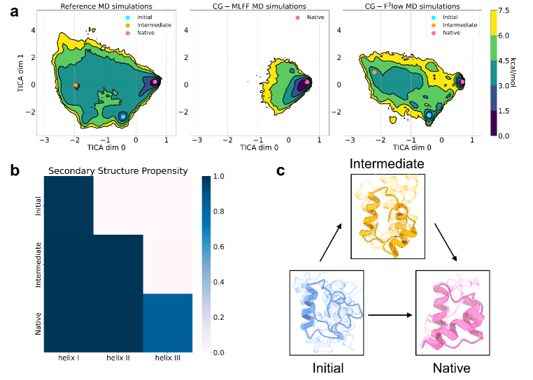
To demonstrate the capabilities of the F3low in exploring conformational space, we took the Homeodomain as a case study. The conformational landscape explored by the CG-F3low exhibited a similar feature as the reference all-atom MD simulations, successfully identifying three metastable states. On the contrary, the CG-MLFF was confined to a single metastable state (Figure 4(a)). Furthermore, the Homeodomain (54 AA in total) is structured into a three-helix bundle, specifically helix I (8-20 AA), helix II (26-36 AA), and helix III (40-53 AA). Notably, helices I and III together form a Helix-Turn-Helix (HTH) motif, a signature motif of DNA-binding proteins and known for its fast-folding properties. Experiment results showed that the HTH motif is more prone to instability than helix I, and the unfolding pathway preferentially disrupts the HTH motif before helix I (Mayor et al. (2000)). Our simulations corroborate these observations, further offering insights into its folding pathway (Figure 4(b) and (c)). From the representative conformational ensembles, it is inferred that helix I appears in all states, even in the unstructured initial microstate. Subsequently, it could transition to an intermediate state, wherein the secondary structures of helix I and helix II are nearly formed, and the tertiary interactions are partially established. Such findings support the hypothesis that the Homeodomain employs a diffusion-collision mechanism for folding. In the mechanism, the secondary structural elements first form independently and later assemble to the tertiary structure, aligning with prior studies of Homeodomain (Mayor et al. (2000); DeMarco et al. (2004)).
Appendix D Experiment details
D.1 Trajectory Dataset
We adopt the large-scale all-atom molecular dynamics dataset in Majewski et al. (2023), which contains twelve fast-folding proteins studied by Lindorff-Larsen et al. (2011). These proteins exhibit diverse secondary structural elements, including -helices and -strands, with lengths spanning from 10 to 80 amino acids. The evaluation of the proposed methods is conducted on three specific protein trajectories selected from the dataset, which are Chignolin (10AA), Trpcage (20AA), and Homeodomain (54AA). Other settings are shown in Table 3.
| Protein | Sequence length (#AA) | Aggregated time () | Min. RMSD (Å) |
|---|---|---|---|
| Chignolin | 10 | 186 | 0.15 |
| Trpcage | 20 | 195 | 0.45 |
| Homeodomain | 54 | 198 | 0.56 |
D.2 Training details
We employ the FramePred model architecture from Yim et al. (2023b), which stacks multiple Invariant Point Attention layers introduced by AlphaFold2 Jumper et al. (2021), which encodes the structural features and decodes the rigid postures in an equivariant way. Additionally, we augment the model with sequence embedding as single features for input. All other model hyperparameters follow Yim et al. (2023a). For guided flow, we set initial guess weight to , guidance weight to 1 and unconditional probability to , in order to conduct a fully guided frame-to-frame simulation. We would explore the effect of and in the future. The training configuration includes a maximum of training epoch, a learning rate of . For Chignolin and Trpcage, a batch size of is employed, while for Homeodomain, a batch size of is utilized. All training experiments are performed individually on a single NVIDIA GeForce RTX 4090 GPU.
D.3 Simulation details
After training, we executed 8 parallel coarse-grained simulations (sampling procedures) with 150,000 samples per protein. These simulations were initiated from conformational states that were randomly selected from the reference free energy surface within the test set. To remove the effect of the starting conformations, we removed the first 10% of sample points per trajectory when plotting the free energy surfaces. All simulation experiments are performed individually on a single NVIDIA GeForce RTX 4090 GPU. The simulation time per step is reported in Table 4.
| Chignolin | Trpcage | Homeodomain | |
|---|---|---|---|
| Simulation time per step (s) | 0.32 0.01 | 0.34 0.01 | 0.38 0.01 |