Soft Preference Optimization: Aligning Language Models to Expert Distributions

Abstract

We propose Soft Preference Optimization (SPO), a method for aligning generative models, such as Large Language Models (LLMs), with human preferences, without the need for a reward model. SPO optimizes model outputs directly over a preference dataset through a natural loss function that integrates preference loss with a regularization term across the model’s entire output distribution rather than limiting it to the preference dataset. Although SPO does not require the assumption of an existing underlying reward model, we demonstrate that, under the Bradley-Terry (BT) model assumption, it converges to a softmax of scaled rewards, with the distribution’s “softness" adjustable via the softmax exponent, an algorithm parameter. We showcase SPO’s methodology, its theoretical foundation, and its comparative advantages in simplicity, computational efficiency, and alignment precision.

1 Introduction

The alignment problem focuses on adjusting a generative model (e.g., Large Language Models (LLMs)) to align its outputs with human preferences and ethical standards or to tailor the model for specific tasks; and is especially important after supervised fine-tuning on datasets with mixed-quality samples. A widely embraced approach involves refining these models based on expert (i.e., human) preferences, typically expert-provided comparisons of pairs of model-generated outputs [1]. Given a preference dataset $\mathcal{D}$ and a pre-trained model $\pi_{\textrm{ref}}$, preference alignment seeks to train a new model, $\pi_{\theta}$, whose outputs are better aligned with the preference in $\mathcal{D}$ [2, 3]. A notable advancement in this field has been the application of Reinforcement Learning from Human Feedback (RLHF), which involves training a reward-model based of actions preferred by humans and then optimizing $\pi_{\theta}$ to maximize these learned rewards while ensuring closeness to the initial model behaviors [4]. Despite the effectiveness of RLHF in addressing the alignment problem, RLHF involves a relatively complex pipeline, susceptible to propagation of reward-model’s biases over to the policy optimization.

Recently, several studies have introduced methods for the direct optimization of preferences, including Direct Preference Optimization (DPO) among others [5, 6, 7, 8, 9, 10, 11]. These approaches eliminate the need for a separate reward model training phase, instead adjusting the model directly using preference data, and often outperform RLHF-based approaches. These reward-model-free methods enjoy advantages over RLHF-based approaches, such as simplified pipelines, reduced computational complexity, and avoidance of the bias transfer from the reward model to policy optimization. Indeed, the rationale for incorporating an additional component, the reward model, into a supervised learning context with a supervised dataset, is debatable.

In this work, we propose a simple and effective reward-model-free alignment method, termed Soft Preference Optimization (SPO). SPO seeks to align the model’s preference estimates (detailed in Section 3) with expert preferences $\mathcal{D}$, through minimizing a loss function of the form

$$\textrm{AlignmentLoss}(\pi_{\theta},\pi_{\textrm{ref}},\mathcal{D})=\textrm{PreferenceLoss}(\pi_{\theta},\mathcal{D})+\textrm{Regularizer}(\pi_{\theta},\pi_{\textrm{ref}}),$$ (1)

where the Regularizer may be chosen as the KL divergence. We discuss natural choices for the model’s preference estimates and the preference loss function in Sections 3 and 4.

Unlike RLHF and DPO, the development of SPO does not rely on assumptions regarding the existence of underlying rewards, such as the Bradley-Terry (BT) model [12]. Nevertheless, we demonstrate that if the BT model is applicable and given an asymptotically large preference dataset, SPO is theoretically guaranteed to converge to a softmax of the rewards, which inspires the designation “Soft Preference Optimization”. Unlike DPO, which tends toward a deterministic model even with an extremely large dataset if the regularization coefficient is nearly zero [13], SPO allows for the adjustment of the softmax’s exponent through an input parameter, thereby offering flexibility in modulating the “softness" of the output distribution.

SPO has two main distinctions from existing reward-model-free alignment methods. The first distinction involves the choice of a preference loss that aligns model’s preference estimates with expert’s preferences, resulting in a favorable fixed point as discussed in the previous paragraph. The other distinction of SPO with DPO and similar algorithms lies in the application of regularization. DPO restricts regularization to the preference dataset, which is counter-intuitive since the dataset already provides specific data points for the model to fit; thus, additional regularization within this limited scope is unnecessary. More critically, since the preference dataset represents a tiny subset of the potential outputs of the model, focusing regularization solely within this subset can lead to undesirable, extensive shift in the model’s distribution outside of the dataset, resulting in a non-coherent behaviours. Acknowledging this limitation, SPO applies regularization across the entire output distribution of the model, not just within the confines of the preference dataset.

2 Background

Consider a finite context (or query) space $\mathcal{X}$ and a finite action (or response) space $\mathcal{Y}$. For a given query $x\in\mathcal{X}$, a behavior policy (such as a pre-trained model) is employed to generate responses $y_{1},y_{2}\in\mathcal{Y}$. These responses are subsequently evaluated by expert raters (e.g., humans) to determine which of $y_{1}$ or $y_{2}$ constitutes a more appropriate response to the query $x$. We adopt the notation $y_{1}\succ y_{2}$ to denote that $y_{1}$ is preferred over $y_{2}$ in a specific context. The true expert preferences are typically represented by a probability, $p^{*}(y_{1}\succ y_{2}|x)$, reflecting the inherent randomness due to the variable nature of the experts, who may be a group of humans with slightly differing preferences. A preference dataset, $\mathcal{D}$, is compiled by collecting expert preferences for multiple $(x;y_{1},y_{2})$ tuples. In detail, $\mathcal{D}$ comprises tuples $(x;y_{w},y_{l})$, where $y_{w}\succ y_{l}$ indicates the preferred (winner) and less preferred (loser) responses based on expert evaluations.

RLHF comprises two main phases: reward modeling and reinforcement learning (RL) fine-tuning. The initial phase, reward modeling, operates under the assumption that there exist latent rewards $r(y|x)$ that form the basis of expert preferences. This phase aims to develop a model capable of closely approximating these underlying rewards. A widely accepted method for defining these latent rewards is through the Bradley-Terry (BT) model [12], alongside the Plackett-Luce (PL) ranking models [14, 15]. The BT model posits that the distribution of expert preferences, $p^{*}$, is characterized by

$$p^{\mathrm{BT}}(y_{1}\succ y_{2}|x)\overset{\text{\tiny def}}{=}\sigma\big{(}r(y_{1}|x)-r(y_{2}|x)\big{)}=\frac{\exp\big{(}r(y_{1}|x)\big{)}}{\exp\big{(}r(y_{1}|x)\big{)}+\exp\big{(}r(y_{2}|x)\big{)}},$$ (2)

where $\sigma(\cdot)$ represents the sigmoid function. Subsequently, the reward model $r_{\phi}(y|x)$ is trained to minimize the negative log-likelihood loss, $-\mathbb{E}_{(x;y_{w},y_{l})\sim\mathcal{D}}\big{[}\sigma\big{(}r(y_{w}|x)-r(y_{l}|x)\big{)}\big{]}$. The PL model generalizes the BT model for data involving rankings, modeling the expert distribution as

$$p^{\mathrm{PL}}(y_{1}\succ\cdots\succ y_{n}\,|\,x)\,\overset{\text{\tiny def}}{=}\,\prod_{k=1}^{n-1}\frac{\exp\big{(}r(y_{k}|x)\big{)}}{\sum_{i=k}^{n}\exp\big{(}r(y_{i}|x)\big{)}},$$ (3)

for all $(x;y_{1},\ldots,y_{n})\in\mathcal{X}\times\mathcal{Y}^{n}$.

The RL fine-tuning phase aims to train a model, $\pi_{\theta}$, to maximize a loss function of the form

$$\mathcal{L}_{\mathrm{RLHF}}\big{(}\pi_{\theta},\pi_{\textrm{ref}},r_{\phi}\big{)}=-\mathbb{E}_{x\sim\mathcal{D},y\sim\pi_{\theta}(\cdot|x)}\big{[}r_{\phi}(y|x)\big{]}+\beta\mathcal{D}_{\textrm{KL}}\big{(}\pi_{\theta}\parallel\pi_{\textrm{ref}}\big{)},$$ (4)

where $\beta$ is a non-negative constant, $r_{\phi}$ is the trained reward function, and $\pi_{\mathrm{ref}}$ is a reference policy often acquired through supervised fine-tuning on high-quality data and is typically identical to the behavior policy. The $D_{KL}$ term in the loss function acts as a regularizer, ensuring the model does not significantly deviate from the distribution where the reward model is most accurate. RL fine-tuning employs reinforcement learning algorithms, like PPO [16], to optimize the above loss function [4], introducing significant complexity into the RLHF pipeline. Additionally, the RLHF framework allows for the propagation of any generalization errors from the reward model to the RL fine-tuned model. The DPO framework [5] addresses these challenges by simplifying the problem into a single-phase supervised learning approach, thus avoiding the pitfalls associated with separate reward modeling and RL fine-tuning phases.

DPO circumvents the need for a reward model by directly optimizing the following loss function:

$$\mathcal{L}_{\mathrm{DPO}}\big{(}\pi_{\theta},\pi_{\textrm{ref}},\mathcal{D}\big{)}=-\mathbb{E}\left[\log\,\sigma\left(\beta\log\frac{\pi_{\theta}(y_{w}|x)}{\pi_{\textrm{ref}}(y_{w}|x)}-\beta\log\frac{\pi_{\theta}(y_{l}|x)}{\pi_{\textrm{ref}}(y_{l}|x)}\right)\right].$$ (5)

It was demonstrated in [5] that $\mathcal{L}_{\mathrm{DPO}}$ has the same minimizer as $\mathcal{L}_{\mathrm{RLHF}}$, under the conditions of the BT model, an asymptotically large dataset, and a sufficiently large model capacity (i.e., a tabular model that encodes the probability of $\pi_{\theta}(y|x)$ for all $x\in\mathcal{X}$ and $y\in\mathcal{Y}$ into a vector). The DPO framework was further extended in [13], aiming to directly maximize the win-rate of $\pi_{\theta}$ against $\pi_{\textrm{ref}}$.

3 SPO - Basic

Following (1), we consider a loss function of the form:

$$\mathcal{L}_{\mathrm{SPO}}(\pi_{\theta},\pi_{\textrm{ref}},\mathcal{D})\,=\,\mathcal{L}_{\mathrm{pref}}(\pi_{\theta},\mathcal{D})\,+\,\mathrm{Reg}(\pi_{\theta},\pi_{\textrm{ref}}),$$ (6)

where $\mathcal{L}_{\mathrm{pref}}$ and $\mathrm{Reg}$ stand for preference loss and regularizer, respectively. We proceed to further detail these components.

The regularization term, $\mathrm{Reg}(\pi_{\theta},\pi_{\textrm{ref}})$, aims to ensure that $\pi_{\theta}$ avoids producing outputs that are highly improbable under $\pi_{\textrm{ref}}$. A common and effective choice is the KL divergence, $\mathcal{D}_{\textrm{KL}}(\pi_{\theta}\parallel\pi_{\textrm{ref}})$, although other regularization options are viable [17]. Importantly, $\mathrm{Reg}(\pi_{\theta},\pi_{\textrm{ref}})$ does not incorporate the preference dataset $\mathcal{D}$ as an input. This is because within $\mathcal{D}$, the model aims to fit to the target preferences, making additional regularization within $\mathcal{D}$ unnecessary. In fact, the regularization term primarily aims to regularize $\pi_{\theta}$ outside $\mathcal{D}$. This approach diverges from the DPO and several other existing loss functions (detailed in Section 8), which only consider the divergence of $\pi_{\theta}$ from $\pi_{\textrm{ref}}$ within the preference dataset.

We now turn our attention to the preference loss. Given a query $x$, let $\pi_{\theta}(y|x)$ denote the probability that model $\pi_{\theta}$ generates output $y$. When presented with a query $x$ and two responses, $y_{1}$ and $y_{2}$, we define the probability that $\pi_{\theta}$ prefers $y_{1}$ over $y_{2}$ as

$$\begin{split}\mathcal{P}_{\pi_{\theta}}(y_{1}\succ y_{2}\mid x)&\overset{\text{\tiny def}}{=}\mathrm{P}\big{(}\textrm{output of }\pi_{\theta}(\cdot|x)\textrm{ is }y_{1}\,\,\big{|}\,\,\textrm{output of }\pi_{\theta}(\cdot|x)\textrm{ is in }\{y_{1},y_{2}\}\big{)}\\ &=\frac{\pi_{\theta}(y_{1}|x)}{\pi_{\theta}(y_{1}|x)+\pi_{\theta}(y_{2}|x)},\end{split}$$ (7)

where the last equality follows from the definition of conditional probability. We can then employ log-likelihood loss to measure the alignment of preference-probabilities’ with the preference-dataset labels,

$$-\mathbb{E}_{(x;y_{w},y_{l})\sim\mathcal{D}}\big{[}\log\,\mathcal{P}_{\pi_{\theta}}(y_{w}\succ y_{l}\mid x)\big{]}.$$ (8)

We consider a preference loss $\mathcal{L}_{\mathrm{pref}}^{\alpha}(\pi_{\theta},\mathcal{D})$ that extends the above cross entropy loss by employing arbitrary exponents for $\pi_{\theta}$. Specifically, we let for any $\alpha>0$,

$$\mathcal{L}_{\mathrm{pref}}^{\alpha}(\pi_{\theta},\mathcal{D})\overset{\text{\tiny def}}{=}-\frac{1}{\alpha}\mathbb{E}_{(x;y_{w},y_{l})\sim\mathcal{D}}\left[\log\,\frac{\pi_{\theta}(y_{w}\mid x)^{\alpha}}{\pi_{\theta}(y_{w}\mid x)^{\alpha}+\pi_{\theta}(y_{l}\mid x)^{\alpha}}\right],$$ (9)

and for $\alpha=0$,

$$\mathcal{L}_{\mathrm{pref}}^{0}(\pi_{\theta},\mathcal{D})\overset{\text{\tiny def}}{=}-\frac{1}{2}\mathbb{E}_{(x;y_{w},y_{l})\sim\mathcal{D}}\left[\log\,\frac{\pi_{\theta}(y_{w}\mid x)}{\pi_{\theta}(y_{l}\mid x)}\right].$$ (10)

This $\mathcal{L}_{\mathrm{pref}}^{\alpha}(\pi_{\theta},\mathcal{D})$ contains the cross-entropy loss in (8) as a special case when $\alpha=1$. The $\alpha$ parameter allows for tailoring the model to exhibit different entropies; models minimized under $\mathcal{L}_{\mathrm{pref}}^{\alpha}$ will display higher entropy for larger $\alpha$ values, gradually moving towards a deterministic model akin to DPO as $\alpha$ approaches zero; as established in the next theorem.

Although the SPO framework does not rely on existence of underlying reward functions, and in particular the BT assumption, it is insightful to study the preference loss $\mathcal{L}_{\mathrm{pref}}^{\alpha}$ under the conditions where the BT model assumption is valid. Intuitively, for a BT expert model, defined as $\pi(y|x)=\exp(r(y|x))/Z(x)$ with $Z(x)$ being the partition function, the preference probability in (7) would be identical to the BT preference formula (2). In the next theorem, we further study the landscape of $\mathcal{L}_{\mathrm{pref}}^{\alpha}$ under the BT model assumption. To eliminate local minima and saddle points that arise from nonlinear model spaces such as neural networks, in the theorems we consider a tabular model that encodes the probability of $\pi_{\theta}(y|x)$ for all $x\in\mathcal{X}$ and $y\in\mathcal{Y}$ into a large vector.

Theorem 1.

Suppose that the BT model holds with rewards $r(\cdot|x)$, and fix any probability distribution $\mathcal{D}$ over $\mathcal{X}\times\mathcal{Y}\times\mathcal{Y}$ that has full support and is consistent with the BT assumption. Then, for any $\alpha\geq 0$, in the tabular model, $\mathcal{L}_{\mathrm{pref}}^{\alpha}$ has a unique minimizer $\operatorname{Softmax}(r(\cdot|x)/\alpha)$ (reducing to $\operatorname{argmax}r(\cdot|x)$ for $\alpha=0$). Furthermore, this minimizer is globally absorbing, and the landscape of $\mathcal{L}_{\mathrm{pref}}^{\alpha}$ contains no other first-order stationary point (i.e., no other local minima, local maxima, or saddle points).

The proof is provided in Appendix A. According to Theorem 1, minimizer of $\mathcal{L}_{\mathrm{pref}}^{\alpha}$ is the softmax of BT rewards divided by $\alpha$, where $\alpha$ controls the entropy of the final model. Specifically, in the the asymptotically large dataset regime, when $\alpha=1$, the preference loss reaches its minimum at the hypothetical BT expert model that generates the preference dataset’s labels, defined as $\operatorname{Softmax}(r(\cdot|x))$.

The gradient of the preference loss $\mathcal{L}_{\mathrm{pref}}^{\alpha}$, for any $\alpha\geq 0$, is given by

$$-\nabla_{\theta}\mathcal{L}_{\mathrm{pref}}^{\alpha}(\pi_{\theta},\mathcal{D})=\mathbb{E}_{(x;y_{w},y_{l})\sim\mathcal{D}}\left[\frac{\pi_{\theta}(y_{l}|x)^{\alpha}}{\pi_{\theta}(y_{w}|x)^{\alpha}+\pi_{\theta}(y_{l}|x)^{\alpha}}\big{(}\nabla_{\theta}\log\pi_{\theta}(y_{w}|x)-\nabla_{\theta}\log\pi_{\theta}(y_{l}|x)\big{)}\right].$$

Here, $\pi_{\theta}(y_{l}|x)^{\alpha}/\big{(}\pi_{\theta}(y_{w}|x)^{\alpha}+\pi_{\theta}(y_{l}|x)^{\alpha}\big{)}$ serves as a measure of the model’s error in preferring $y_{w}$ over $y_{l}$. Consequently, the magnitude of this preference error proportionally scales the adjustment $\nabla_{\theta}\log\,\pi_{\theta}(y_{w}|x)-\nabla_{\theta}\log\,\pi_{\theta}(y_{l}|x)$, leading to larger updates when the error is large.

4 SPO - Weighted

We further expand the preference loss of SPO by considering a weighting over different samples, where the weights can depend on $\pi_{\theta}$. This weighting only affects (improves) the optimization process without changing the fixed point, as we show in this section.

We call a function $\mu:\mathcal{Y}\times\mathcal{Y}\times\mathcal{X}\to\mathbb{R}^{+}$ symmetric positive if $\mu(y_{1},y_{2}\mid x)=\mu(y_{2},y_{1}\mid x)>0$, for all $x\in\mathcal{X}$ and all $y_{1},y_{2}\in\mathcal{Y}$. Given a symmetric positive function $\mu$ and an $\alpha\geq 0$, we define weighted preference loss as

$$\mathcal{L}_{\mathrm{pref}}^{\alpha,\mu}(\pi_{\theta},\mathcal{D})\overset{\text{\tiny def}}{=}-\frac{1}{\alpha}\mathbb{E}_{(x;y_{w},y_{l})\sim\mathcal{D}}\left[\mu(y_{w},y_{l}\mid x)\,\log\,\frac{\pi_{\theta}(y_{w}\mid x)^{\alpha}}{\pi_{\theta}(y_{w}\mid x)^{\alpha}+\pi_{\theta}(y_{l}\mid x)^{\alpha}}\right]$$ (11)

if $\alpha>0$, and for $\alpha=0$ we let

$$\mathcal{L}_{\mathrm{pref}}^{0,\mu}(\pi_{\theta},\mathcal{D})\overset{\text{\tiny def}}{=}-\frac{1}{2}\mathbb{E}_{(x;y_{w},y_{l})\sim\mathcal{D}}\left[\mu(y_{w},y_{l}\mid x)\,\log\,\frac{\pi_{\theta}(y_{w}\mid x)}{\pi_{\theta}(y_{l}\mid x)}\right].$$ (12)

The weight-function $\mu$ controls the impact of individual samples within the loss calculation. The utility of $\mu$ emerges from the observation that not all sample pairs in the preference dataset hold equivalent significance. For instance, diminishing the weights of dataset samples $(x;y_{w},y_{l})$ where both responses $y_{w}$ and $y_{l}$ are of low quality (e.g., low probability) can be particularly advantageous. This can be achieved for example by setting $\mu(y_{w},y_{l}\mid x)\propto\big{(}\pi_{\theta}(y_{w}\mid x)+\pi_{\theta}(y_{l}\mid x)\big{)}^{\gamma}$, with $\gamma>0$.

While $\mu$ may depend on $\pi_{\theta}$, it is important to note that gradient propagation through $\mu$ is not permitted. Specifically, the gradient $\nabla_{\theta}\mathcal{L}_{\mathrm{pref}}^{\alpha,\mu}(\pi_{\theta},\mathcal{D})$ is given by

$$-\mathbb{E}_{(x;y_{w},y_{l})\sim\mathcal{D}}\left[\mu(y_{w},y_{l}|x)\,\frac{\pi_{\theta}(y_{l}|x)^{\alpha}}{\pi_{\theta}(y_{w}|x)^{\alpha}+\pi_{\theta}(y_{l}|x)^{\alpha}}\,\big{(}\nabla_{\theta}\log\,\pi_{\theta}(y_{w}|x)-\nabla_{\theta}\log\,\pi_{\theta}(y_{l}|x)\big{)}\right].$$ (13)

Interestingly, the weight function, $\mu$, mainly influences the optimization process, not the ultimate fixed point, in the tabular setting and under asymptotically large preference dataset, as we show in the next theorem.

Theorem 2.

Suppose that the conditions of Theorem 1 hold. Then for any $\alpha\geq 0$ and any symmetric positive function $\mu$, the softmax of the BT rewards divided by $\alpha$, $\operatorname{Softmax}(r(\cdot|x)/\alpha)$ (reducing to $\operatorname{argmax}r(\cdot|x)$ for $\alpha=0$), is the unique globally absorbing fixed point of the differential equation $\dot{\boldsymbol{\pi}}=\prod\big{(}-\nabla_{\theta}\mathcal{L}_{\mathrm{pref}}^{\alpha,\mu}(\pi_{\theta},\mathcal{D})\big{)}$, where $\prod(\cdot)$ stands for projection onto the probability simplex, and the gradient is given in (13).

The proof is given in Appendix A.

5 SPO for Other Data-Types: Best-of-$n$ Preference and Ranked Preference

In this section, we generalize the SPO algorithm for other types of preference data: best-of-$n$ preference data and ranked-data. We extend the definition of a symmetric function to $n$-responses by calling a function $\mu:\mathcal{Y}^{n}\times\mathcal{X}\to\mathbb{R}^{+}$ symmetric positive if $\mu(y_{\tau(1)},\ldots,y_{\tau(n)}\mid x)=\mu(y_{1},\ldots,y_{n}\mid x)>0$, for all $x\in\mathcal{X}$ all $y_{1},\ldots,y_{n}\in\mathcal{Y}$, and all permutations $\tau$ of $(1,\ldots,n)$.

Best-of-$n$ preference data: Given an $n\geq 2$, a sample $(x;y_{1},\ldots,y_{n};i^{*})$ of a best-of-$n$ preference dataset consists of a query $x$ along with $n$ responses $y_{1},\ldots,y_{n}$, one of which (i.e., $y_{i^{*}}$) is labeled by the expert as the best response. Given a symmetric positive function $\mu$ and an $\alpha>0$, we propose the following preference loss for a best-of-$n$ preference dataset $\mathcal{D}$:

$$\mathcal{L}_{\mathrm{pref}\textrm{-}n}^{\alpha,\mu}(\pi_{\theta},\mathcal{D})\overset{\text{\tiny def}}{=}-\frac{1}{\alpha}\mathbb{E}_{(x;y_{1},\ldots,y_{n};i^{*})\sim\mathcal{D}}\left[\mu(y_{1},\ldots,y_{n}\mid x)\,\log\,\frac{\pi_{\theta}(y_{i^{*}}\mid x)^{\alpha}}{\sum_{i=1}^{n}\pi_{\theta}(y_{i}\mid x)^{\alpha}}\right].$$ (14)

As before, we stop the gradient from propagating through $\mu$, even though $\mu$ may depend on $\pi_{\theta}$. Similar to the case of pairwise preferences, we show in the following theorem that the loss in (14) is minimized at the softmax of rewards, if we assume existence of an underlying reward function. In particular, given a reward function $r(\cdot|x):\mathcal{X}\to\mathcal{Y}$ and a distribution $\mathcal{D}$ over $\mathcal{X}\times\mathcal{Y}^{n}\times\{1,\ldots,n\}$, we say that $\mathcal{D}$ is consistent with $n$-ary BT model if for any $(x;y_{1},\ldots,y_{n})\in\mathcal{X}\times\mathcal{Y}^{n}$ and any $i,j\in\{1,\ldots,n\}$, $\mathcal{D}(x;y_{1},\ldots,y_{n};i)/\mathcal{D}(x;y_{1},\ldots,y_{n};j)=\exp\big{(}r(y_{i}\mid x)-r(y_{j}\mid x)\big{)}$. Note that this definition boils down to the definition of consistency with BT model for $n=2$ in Section 3. Proof of the following theorem is given in Appendix B.

Theorem 3.

Consider a reward function $r(\cdot\mid x)$ and a probability distribution $\mathcal{D}$ with full support over $\mathcal{X}\times\mathcal{Y}^{n}\times\{1,\ldots,n\}$ that is consistent with the $n$-ary BT model. Then, for any $\alpha>0$ and any symmetric positive function $\mu$, in the tabular model, $\operatorname{Softmax}(r(\cdot|x)/\alpha)$ is the unique globally absorbing fixed point of the differential equation $\dot{\boldsymbol{\pi}}=\prod\big{(}-\nabla_{\theta}\mathcal{L}_{\mathrm{pref}\textrm{-}n}^{\alpha,\mu}(\pi_{\theta},\mathcal{D})\big{)}$, where $\prod(\cdot)$ stands for projection onto the probability simplex.

Ranked Preference Data: A ranked preference dataset consists of samples of the form $(x;y_{1},\ldots,y_{n};\tau)$, where $x$ is a query, $y_{1},\ldots,y_{n}$ are $n$ responses, and $\tau$ is a permutation representing the relative preference $y_{\tau(1)}\succ\cdots\succ y_{\tau(n)}$ of the expert over these responses. Given an $\alpha>0$ and a sequence of symmetric positive function $\mu_{k}:\mathcal{X}\times\mathcal{Y}^{k}\to\mathbb{R}$ for $k=2,\ldots,n$, we propose the following preference loss for a ranked preference dataset $\mathcal{D}$:

$$\mathcal{L}_{\mathrm{rank}}^{\alpha,[\mu]}(\pi_{\theta},\mathcal{D})\overset{\text{\tiny def}}{=}-\frac{1}{\alpha}\mathbb{E}_{(x;y_{1},\ldots,y_{n};\tau)\sim\mathcal{D}}\left[\sum_{k=1}^{n-1}\mu_{k}(y_{\tau(k)},\ldots,y_{\tau(n)}|x)\,\log\,\frac{\pi_{\theta}(y_{\tau(k)}\,|\,x)^{\alpha}}{\sum_{j=k}^{n}\pi_{\theta}(y_{\tau(j)}\,|\,x)^{\alpha}}\right].$$ (15)

We can control the importance weight of responses in different ranks through appropriate adjustment of weight functions $\mu^{1},\ldots,\mu^{n-1}$. For example, by setting $\mu_{k}=0$ for $k=2,\ldots,n-1$, $\mathcal{L}_{\mathrm{rank}}^{\alpha,[\mu]}$ boils down to $\mathcal{L}_{\mathrm{pref}\textrm{-}n}^{\alpha,\mu^{1}}$. Here again, the gradient is not allowed to propagate through $\mu^{1},\ldots,\mu^{n-1}$, even though these functions may depend on $\pi_{\theta}$. The following theorem shows that, assuming existence of underlying rewards under the PL model (3), the softmax of these rewards is the unique minimizer of $\mathcal{L}_{\mathrm{rank}}^{\alpha,\mu}$. The proof relies on Theorem 3, and is given in Appendix C.

Theorem 4.

Suppose that the PL model holds with rewards $r(\cdot|x)$, and a probability distribution $\mathcal{D}$ with full support over $\mathcal{X}\times\mathcal{Y}^{n}\times\{\mathrm{Identity\,permutation}\}$ that is consistent with the PL model. Then, for any $\alpha>0$ and any sequence $[\mu]=\mu^{1},\ldots,\mu^{n-1}$ of symmetric positive functions, in the tabular model, $\operatorname{Softmax}(r(\cdot|x)/\alpha)$ is the unique globally absorbing fixed point of the differential equation $\dot{\boldsymbol{\pi}}=\prod\big{(}-\nabla_{\theta}\mathcal{L}_{\mathrm{rank}}^{\alpha,[\mu]}(\pi_{\theta},\mathcal{D})\big{)}$, where $\prod(\cdot)$ stands for projection onto the probability simplex.

6 Comparative Analysis: SPO Versus DPO

This section contrasts the SPO method with the DPO algorithm, at a conceptual level. A detailed empirical comparison with DPO will follow in Section 7.

A key distinction between SPO and DPO lies in the application of the regularization (or $\mathcal{D}_{\textrm{KL}}(\pi_{\theta}\parallel\pi_{\textrm{ref}})$). The DPO loss function (5) incorporates regularization over preference dataset samples only. This approach is suboptimal since the primary objective of alignment is to align with the preferences in the dataset, and regularization within the preference dataset undermines this objective. The inclusion of $\mathcal{D}_{\textrm{KL}}$ in RLHF originally aimed to mitigate the risk of $\pi_{\theta}$ diverging significantly from $\pi_{\textrm{ref}}$ in unexplored regions of the response space, which could lead to unexpected distribution shifts. In the same vein, SPO incorporates a global regularizer, acting across the entire response space rather than being confined to the preference dataset.

Another advantage of SPO over DPO and RLHF emerges from the tendency of DPO and RLHF models towards determinism. Consider a hypothetical scenario where the preference dataset is significantly larger compared to the data used for pre-training. In such a context, the preference dataset itself provides ample information for model alignment, rendering the regularization or $\mathcal{D}_{\textrm{KL}}$ unnecessary; equivalently $\beta$ can be set to a very small value or zero. In this case, under BT-model assumption, the minimizers of the RLHF and DPO loss functions are deterministic models that for each query $x$, deterministically return a response $y$ that maximizes $r(y|x)$. In general, the RLHF and DPO loss functions have an inherent tendency towards low entropy policies [13], which results in a constrained range of responses, leading to potential mode collapse, where the model’s outputs, although high-quality, are limited to a narrow set. In contrast, SPO, through its alignment loss in (6), allows for entropy control of the output solution via the $\alpha$ parameter in (9), even when $\beta=0$ (see Theorem 1). This capacity to preserve information diversity makes SPO more adaptable for continual learning scenarios, enabling the model to evolve over time and be applied to subsequent alignments without significant loss of potential sets of responses.

It is noteworthy that unlike RLHF and DPO, the SPO framework does not presuppose the existence of an underlying reward model nor relies on assumptions such as the BT model. Instead, SPO’s preference loss aims to directly align $\pi_{\theta}$ with the preferences in the preference dataset. This distinction potentially facilitates the adaptation of SPO to broader alignment contexts. Furthermore, the choice of regularization is not confined to $\mathcal{D}_{\textrm{KL}}$. This stands in contrast to the DPO and IPO frameworks, which fundamentally depend on employing $\mathcal{D}_{\textrm{KL}}$ for derivation of their loss functions.

We further observe that the DPO loss does not allow for separation into components like (6), namely as a sum of a preference loss that is independent of $\pi_{\textrm{ref}}$ and a regularizer such as $\mathcal{D}_{\textrm{KL}}$. To understand why, consider a scenario where $\pi_{\theta}(y_{w}|x)=\pi_{\theta}(y_{l}|x)$ for a given sample $(x;y_{w},y_{l})\in\mathcal{D}$. In this instance, the alignment loss remains symmetrical with respect to $\pi_{\textrm{ref}}(y_{w}|x)$ and $\pi_{\textrm{ref}}(y_{l}|x)$; because swapping the values of $\pi_{\textrm{ref}}(y_{w}|x)$ and $\pi_{\textrm{ref}}(y_{l}|x)$ would not alter either the preference loss or $\mathcal{D}_{\textrm{KL}}$. This symmetry is absent in the DPO framework, as evident from the DPO loss formulation in (5).

Despite the benefits of regularizing $\pi_{\theta}$ across the entire response space, as opposed to restricting $\mathcal{D}_{\textrm{KL}}$ solely to the preference dataset—a point highlighted earlier in this section—this approach can lead to significant computational overhead. This is particularly true for sequential generative models such as language models, where generating sequences is computationally more intensive than calculating the probability of a given sequence. In Appendix D, we discuss methods to resolve this and other practical concerns of SPO.

7 Experiments

We evaluated the performance of SPO in a story generation task, using pre-trained models on the TinyStories dataset [18] which is a synthetic collection of brief stories designed for children aged 3 to 4. This dataset proves effective for training and evaluating language models that are smaller than the current state-of-the-art, and capable of crafting stories that are not only fluent and coherent but also diverse. We created a preference dataset for aligning the stories to older age groups. The dataset consists of approximately 100,000 story-pairs labeled by GPT3.5 Turbo. Further details are provided in Appendix E.1.

Building on the implementation in [19], and initializing by the supervised fine tuned (SFT) model from [20], we aligned a 110M parameter model using SPO (in particular, the basic unweighted version of SPO presented in Section 3) and three state-of-the-art alignment methods: DPO [5], IPO [13], and SLiC-HF [21]. For all algorithms, the reference model was chosen identical to the SFT model. Refer to Appendix E.2 for further implementation details.

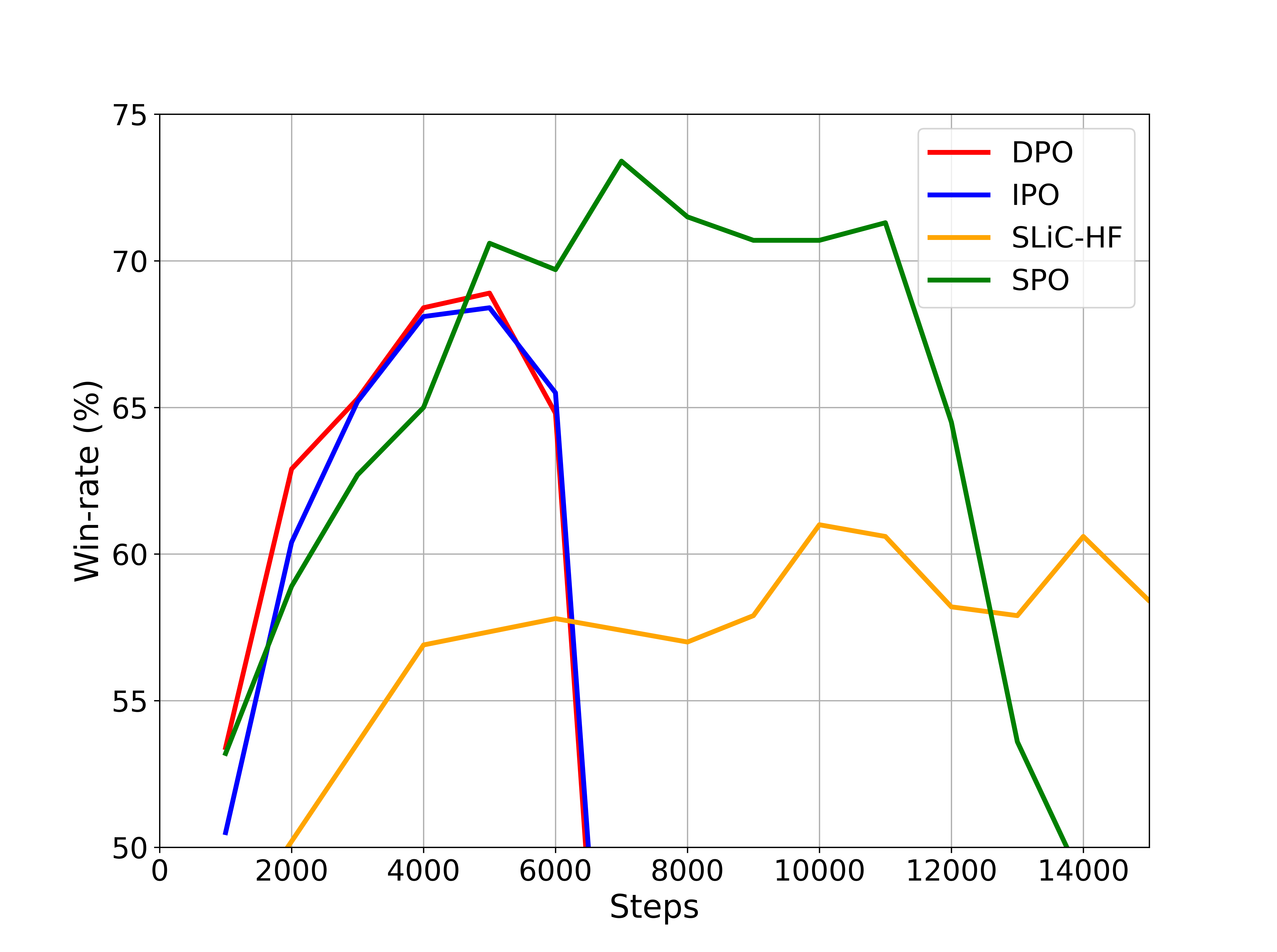
Figure 1: Win-rates of different alignment methods versus number of steps.

Table 1 shows peak win-rates against the SFT model, for different alignment algorithms. According to Table 1, the peak win-rate of SPO surpasses all baselines by a $4.5\%$ margin. Figure 1 illustrates the win rates versus training steps. SPO demonstrates a higher and wider peak, as well as much less sensitivity to over-training, compared to DPO and IPO. Specifically, the win-rate of DPO and IPO quickly drops below $30\%$ after a narrow peak, whereas the win-rate of SPO after over-training fluctuates around $50\%$ for a long time. Refer to Appendix E.3 for complementary demonstrations and details.

Table 1: Win-rate against the SFT model, for different alignment methods.

Alignment method	Win-rate (%)
DPO [5]	68.9
IPO [13]	68.4
SLiC-HF [21]	61
SPO (our work)	73.4

8 Related Works

RLHF aims to align AI systems with human preferences, relying on human judgments rather than manual rewards or demonstrations. This method has been successfully applied in fine-tuning large language models (LLMs) [22, 23, 4], but faces challenges including data quality issues, reward misgeneralization, and policy optimization complexities. Research to enhance RLHF includes methods such as rejection sampling for response generation [24, 23], where the highest-reward response from a fixed number is selected for fine-tuning. The reference [25] simplified instruction alignment with language models into a goal-oriented reinforcement learning task, utilizing a two-phase approach of high-temperature online sampling and supervised learning with relabeled data during offline training. A two-loop learning algorithm, Grow and Improve, has also been proposed for iterative model alignment and training on a fixed dataset [26]. The Grow loop leverages the existing model to create and sample a dataset while the Improve loop iteratively trains the model on a fixed dataset.

Given the challenges of RLHF, reward-model-free alignment methods emerged fairly recently and have gained a lot of popularity. Reward-model-free approach to alignment was popularized specifically after introduction of DPO in [5], which is breifly outlined in Section 2. Recently, several works have been proposed methods to improve DPO. In [13], the authors considered an objective called $\Psi$PO for learning from human preferences that is expressed in terms of pairwise preferences, with no need for assumption of the BT model. The authors focused on a specific instance, IPO, of $\Psi$PO by setting $\Psi$ as the identity, aiming to mitigate the overfitting and tendency-towards-deterministic-policies issues observed in DPO. In [27], the alignment problem is formulated as finding the Nash equilibrium (NE) of a maximin game with two policies $\pi$ and $\pi^{\prime}$ as two players where each policy receives pay off of probability of winning over the other policy. The author showed that the NE point can be approximated by running a mirror-descent-like algorithm. In [28, 29], other approaches have been proposed to approximate the NE point based on no-regret algorithms [30]. The work in [7] proposed a loss function which is an unbiased estimate of the original DPO loss, and aims to alleviate sensitivity to flipped labels due to labeling noise. It was proposed in [6] to add an offset term within the sigmoid function in the DPO loss. In this manner, the model puts more weight on the winning response. In order to reduce the memory usage of DPO, [8] approximated the DPO loss by replacing $\pi_{\textrm{ref}}$ with a uniform reference model, eliminating the need to store and evaluate the reference model. In [31], a token-level formulation of DPO has been proposed which enables a likelihood search over a DPO model by classical search-based algorithms, such as MCTS. Inspired by cringe loss previously proposed for binary feedback, [10] adapted cringe loss for the pairwise preference context. More specifically, cringe loss applies standard likelihood training to winning responses. For a losing response, it contrasts each token in the losing sequence against other likely tokens predicted by the model, aiming to discourage the losing sequence from being the top-ranked sequence.

In [17], the authors proposed a separable alignment technique, called SLiC, where, similar to SPO, the alignment loss is the sum of two terms: a calibration loss that contrasts a winner and loser responses encouraging the model $\pi_{\theta}$ to assign more probability to the winner, and a regularizer term. SLiC was further developed in [21] to be used in alignment to preference data, where they proposed the SLiC-HF algorithm. SLiC-HF involves a rectified contrastive-loss as its calibration loss and a log-likelihood term as the regularization. Other than a different choices for preference loss and regularization, SLiC-HF diverges from the SPO framework in that the regularization in SLiC-HF is limited to the preference or pre-training datasets, not using online samples from $\pi_{\theta}$ as in the $\mathcal{D}_{\textrm{KL}}$ regularizer.

In practice, the performance of an alignment technique highly depends on the quality of the human preference dataset. Noisy preference pairs could potentially limit the language models from capturing human intention. In [32], DPO was used in conjunction with an improved preference dataset via a rejection sampling technique, arguing that DPO suffers from a mismatch between the sampling distribution and the policy corresponding to true expert preferences. In [11], the authors formed a dataset of conservative pairs by collecting AI feedback through an ensemble of chat model completions, followed by GPT-4 scoring. Then, they employed DPO for alignment to this improved dataset. The work in [9] leveraged semantic correlations of prompts in the dataset to form more conservative response pairs. For a given prompt $(x;y_{w},y_{l})$, a prompt $x^{\prime}$ with a similar semantic to a tuple $(x^{\prime};y^{\prime}_{w},y^{\prime}_{l})$ is used to form more conservative pairs. In particular, they propose a weighted version of the DPO loss where for a given labeled data $(x;y_{w},y_{l})$, $y_{w}$ is approved while $y_{l}$ and any $y^{\prime}_{l}$ (from a similar prompt $x^{\prime}$) are penalized.

9 Limitations

This paper introduced SPO, a class of algorithms designed for alignment to the expert’s distribution, with controlled softness. The paper also presents theoretical results demonstrating favorable landscape and convergence properties of SPO. We find it quite surprising that despite the simplicity, natural formulation, and advantageous theoretical properties of SPO, it has not been proposed or studied before. Below, we discuss the limitations of this work from two perspectives.

Limitations of the SPO Algorithm: The primary limitation of the SPO framework is the computational complexity of the regularizer. Specifically, obtaining a low-variance approximation of $\mathcal{D}_{\textrm{KL}}(\pi_{\theta}\parallel\pi_{\textrm{ref}})$ requires sampling from the current model $\pi_{\theta}$. This process is costly in sequential models, including generative language transformers, where sequence generation necessitates sequential calls to the model. However, this complexity overhead can be mitigated through intermittent generation and large batch processing (discussed in detail in Appendix D), resulting in negligible computational overhead, as we observed in the experiments.

Limitations of the Current Study: In addition to the inherent limitations of the proposed method, this study faces several constraints primarily due to insufficient resources. The most significant limitation is the absence of large-scale experiments. It is important to investigate how these methods scale to larger models and how the performance of different methods varies with the size of the dataset.

Among other interesting problems not addressed in this work, the question of how to generalize to other forms of implicit preference information hidden in the data (e.g., in a chat), rather than labeled preference datasets, represents an intriguing research direction. Additionally, we did not investigate the robustness of the algorithm to noise in the dataset. Studying this aspect and developing methods to enhance the algorithm’s robustness to label noise warrants further research.

Appendices

Appendix A Proof of Theorems 1 and 2

In this appendix, we present the proof of Theorems 1 and 2. The high-level proof idea is to show that moving along the projected negative gradient of the preference loss (i.e., the ODE direction) results in an absolute reduction of the Euclidean distance of $\pi_{\theta}$ from $\operatorname{Softmax}\big{(}r(\cdot|x)/\alpha\big{)}$.

Without loss of generality, we prove the theorem for a single fixed $x\in\mathcal{X}$, and remove $x$ from the notations, for the sake of notation simplicity.

Given the rewards $r(\cdot)$ in the Bradley-Terry model, let

$$\pi^{*}(\cdot)\overset{\text{\tiny def}}{=}\operatorname{Softmax}\big{(}r(\cdot)\big{)}.$$ (16)

For any $\alpha\in[0,1)$, let

$$\pi^{*}_{\alpha}(\cdot)\overset{\text{\tiny def}}{=}\operatorname{Softmax}\big{(}r(\cdot)/\alpha\big{)},$$ (17)

and let $\boldsymbol{\pi}^{\alpha}$ be its vector representation. Therefore, for any $\alpha\in[0,1]$, and for any $y$,

$$\pi^{*}(y)=z_{\alpha}\,\times\,\big{(}\pi^{*}_{\alpha}(y)\big{)}^{\alpha},\qquad\textrm{where }z_{\alpha}\overset{\text{\tiny def}}{=}\frac{\Big{(}\sum_{y^{\prime}}e^{r(y^{\prime})/\alpha}\Big{)}^{\alpha}}{\sum_{y^{\prime}}e^{r(y^{\prime})}}.$$ (18)

Moreover, it follows from the consistency of distribution $\mathcal{D}$ with the Bradley-Terry model that for any pair $(y_{1},y_{2})$,

$$\frac{\mathcal{D}(y_{1},y_{2})}{\mathcal{D}(y_{1},y_{2})+\mathcal{D}(y_{2},y_{1})}=\mathcal{P}_{\mathcal{D}}\big{(}y_{1}\succ y_{2}\big{)}=\frac{\exp{r(y_{1})}}{\exp{r(y_{1})}+\exp{r(y_{2})}}=\frac{\pi^{*}(y_{1})}{\pi^{*}(y_{1})+\pi^{*}(y_{2})}.$$ (19)

For any $y_{1},y_{2}\in\mathcal{Y}$ let

$$\tilde{\mu}(y_{1},y_{2})\overset{\text{\tiny def}}{=}\mu(y_{1},y_{2})\big{(}\mathcal{D}(y_{1},y_{2})+\mathcal{D}(y_{2},y_{1})\big{)}.$$ (20)

Note that the symmetry of $\mu$ implies symmetry of $\tilde{\mu}$ with respect to its first and second arguments. Then,

$$\mu(y_{1},y_{2})\,\mathcal{D}(y_{1},y_{2})=\tilde{\mu}(y_{1},y_{2})\,\frac{\mathcal{D}(y_{1},y_{2})}{\mathcal{D}(y_{1},y_{2})+\mathcal{D}(y_{2},y_{1})}=\tilde{\mu}(y_{1},y_{2})\,\frac{\pi^{*}(y_{1})}{\pi^{*}(y_{1})+\pi^{*}(y_{2})},$$ (21)

where the last equality follows from (19).

Consider a $\boldsymbol{\pi}_{\theta}$ in the relative interior of the probability simplex and let $\mathbf{v}$ be the negative gradient of the preference loss

$$\mathbf{v}\overset{\text{\tiny def}}{=}-\nabla_{\pi_{\theta}}\,\mathcal{L}_{\mathrm{pref}}^{\alpha,\mu}(\pi_{\theta},\mathcal{D}),$$ (22)

where $\mathcal{L}_{\mathrm{pref}}^{\alpha,\mu}$ is defined in (13). For any $y\in\mathcal{Y}$, let $v(y)$ be the entry of $\mathbf{v}$ that corresponds to $y$. Then,

$$\begin{split}v(y)=&\sum_{y^{\prime}\in\mathcal{Y}}\mathcal{D}(y,y^{\prime})\mu(y,y^{\prime})\,\frac{\pi_{\theta}(y^{\prime})^{\alpha}}{\pi_{\theta}(y)^{\alpha}+\pi_{\theta}(y^{\prime})^{\alpha}}\,\left(\frac{d}{d\,\pi_{\theta}(y)}\log\,\pi_{\theta}(y)-\frac{d}{d\,\pi_{\theta}(y)}\log\,\pi_{\theta}(y^{\prime})\right)\\ &+\sum_{y^{\prime}\in\mathcal{Y}}\mathcal{D}(y^{\prime},y)\mu(y^{\prime},y)\,\frac{\pi_{\theta}(y)^{\alpha}}{\pi_{\theta}(y)^{\alpha}+\pi_{\theta}(y^{\prime})^{\alpha}}\,\left(\frac{d}{d\,\pi_{\theta}(y)}\log\,\pi_{\theta}(y^{\prime})-\frac{d}{d\,\pi_{\theta}(y)}\log\,\pi_{\theta}(y)\right)\\ =&\sum_{y^{\prime}\in\mathcal{Y}}\tilde{\mu}(y,y^{\prime})\,\frac{\pi^{*}(y)}{\pi^{*}(y)+\pi^{*}(y^{\prime})}\,\,\frac{\pi_{\theta}(y^{\prime})^{\alpha}}{\pi_{\theta}(y)^{\alpha}+\pi_{\theta}(y^{\prime})^{\alpha}}\,\,\frac{1}{\pi_{\theta}(y)}\\ &-\sum_{y^{\prime}\in\mathcal{Y}}\tilde{\mu}(y,y^{\prime})\,\frac{\pi^{*}(y^{\prime})}{\pi^{*}(y)+\pi^{*}(y^{\prime})}\,\,\frac{\pi_{\theta}(y)^{\alpha}}{\pi_{\theta}(y)^{\alpha}+\pi_{\theta}(y^{\prime})^{\alpha}}\,\,\frac{1}{\pi_{\theta}(y)}\\ =&\sum_{y^{\prime}\in\mathcal{Y}}\,\frac{\tilde{\mu}(y,y^{\prime})\,\big{(}\pi^{*}(y)\pi_{\theta}(y^{\prime})^{\alpha}-\pi^{*}(y^{\prime})\pi_{\theta}(y)^{\alpha}\big{)}}{\pi_{\theta}(y)\,\big{(}\pi^{*}(y)+\pi^{*}(y^{\prime})\big{)}\,\big{(}\pi_{\theta}(y)^{\alpha}+\pi_{\theta}(y^{\prime})^{\alpha}\big{)}},\end{split}$$ (23)

where the first equality follows from (13) and by considering all the terms that include $y$ either as winner (the first sum) or loser (the second sum); the second equality is due to (21) and the fact that $\tilde{\mu}$ is symmetric. To simplify the notation, for any $y$ and $y^{\prime}$, let

$$h(y,y^{\prime})\overset{\text{\tiny def}}{=}\frac{\tilde{\mu}(y,y^{\prime})}{\pi_{\theta}(y)\,\pi_{\theta}(y^{\prime})\,\big{(}\pi^{*}(y)+\pi^{*}(y^{\prime})\big{)}\,\big{(}\pi_{\theta}(y)^{\alpha}+\pi_{\theta}(y^{\prime})^{\alpha}\big{)}}.$$ (24)

Then, (23) simplifies to

$$v(y)=\sum_{y^{\prime}\in\mathcal{Y}}h(y,y^{\prime})\,\pi_{\theta}(y^{\prime})\,\big{(}\pi_{\theta}(y^{\prime})^{\alpha}\pi^{*}(y)-\pi_{\theta}(y)^{\alpha}\pi^{*}(y^{\prime})\big{)}.$$ (25)

Consequently,

$$\begin{split}\mathbf{v}^{T}&(\boldsymbol{\pi}_{\theta}-\boldsymbol{\pi}^{*}_{\alpha})=\sum_{y\in\mathcal{Y}}\,v(y)\,\big{(}\pi_{\theta}(y)-\pi^{*}_{\alpha}(y)\big{)}\\ =&\sum_{y,y^{\prime}\in\mathcal{Y}}\,h(y,y^{\prime})\,\big{(}\pi_{\theta}(y^{\prime})^{\alpha}\pi^{*}(y)-\pi_{\theta}(y)^{\alpha}\pi^{*}(y^{\prime})\big{)}\,\,\pi_{\theta}(y^{\prime})\,\big{(}\pi_{\theta}(y)-\pi^{*}_{\alpha}(y)\big{)}\\ =&\,\,\frac{1}{2}\sum_{y,y^{\prime}\in\mathcal{Y}}\,h(y,y^{\prime})\,\big{(}\pi_{\theta}(y^{\prime})^{\alpha}\pi^{*}(y)-\pi_{\theta}(y)^{\alpha}\pi^{*}(y^{\prime})\big{)}\,\,\pi_{\theta}(y^{\prime})\,\big{(}\pi_{\theta}(y)-\pi^{*}_{\alpha}(y)\big{)}\\ &+\frac{1}{2}\sum_{y^{\prime},y\in\mathcal{Y}}\,h(y^{\prime},y)\,\big{(}\pi_{\theta}(y)^{\alpha}\pi^{*}(y^{\prime})-\pi_{\theta}(y^{\prime})^{\alpha}\pi^{*}(y)\big{)}\,\,\pi_{\theta}(y)\,\big{(}\pi_{\theta}(y^{\prime})-\pi^{*}_{\alpha}(y^{\prime})\big{)}\\ =&\,\,\frac{1}{2}\sum_{y,y^{\prime}\in\mathcal{Y}}\,h(y,y^{\prime})\,\big{(}\pi_{\theta}(y^{\prime})^{\alpha}\pi^{*}(y)-\pi_{\theta}(y)^{\alpha}\pi^{*}(y^{\prime})\big{)}\,\,\,\big{(}\pi_{\theta}(y^{\prime})\pi_{\theta}(y)-\pi_{\theta}(y^{\prime})\pi^{*}_{\alpha}(y)\big{)}\\ &+\frac{1}{2}\sum_{y,y^{\prime}\in\mathcal{Y}}\,h(y,y^{\prime})\,\big{(}\pi_{\theta}(y^{\prime})^{\alpha}\pi^{*}(y)-\pi_{\theta}(y)^{\alpha}\pi^{*}(y^{\prime})\big{)}\,\,\,\big{(}\pi_{\theta}(y)\pi^{*}_{\alpha}(y^{\prime})-\pi_{\theta}(y)\pi_{\theta}(y^{\prime})\big{)}\\ =&\,\,\frac{1}{2}\sum_{y,y^{\prime}\in\mathcal{Y}}\,h(y,y^{\prime})\,\big{(}\pi_{\theta}(y^{\prime})^{\alpha}\pi^{*}(y)-\pi_{\theta}(y)^{\alpha}\pi^{*}(y^{\prime})\big{)}\,\,\,\big{(}\pi_{\theta}(y)\pi^{*}_{\alpha}(y^{\prime})-\pi_{\theta}(y^{\prime})\pi^{*}_{\alpha}(y)\big{)}\\ =&\,-\frac{z_{\alpha}}{2}\sum_{y,y^{\prime}\in\mathcal{Y}}\,h(y,y^{\prime})\,\Big{(}\big{(}\pi_{\theta}(y^{\prime})\pi^{*}_{\alpha}(y)\big{)}^{\alpha}-\big{(}\pi_{\theta}(y)\pi^{*}_{\alpha}(y^{\prime})\big{)}^{\alpha}\Big{)}\,\,\,\big{(}\pi_{\theta}(y^{\prime})\pi^{*}_{\alpha}(y)-\pi_{\theta}(y)\pi^{*}_{\alpha}(y^{\prime})\big{)}\\ =&\,-\frac{z_{\alpha}}{2}\sum_{y,y^{\prime}\in\mathcal{Y}}\,h(y,y^{\prime})\big{(}\pi_{\theta}(y)\pi_{\theta}(y^{\prime})\big{)}^{1+\alpha}\,\left(\left(\frac{\pi^{*}_{\alpha}(y)}{\pi_{\theta}(y)}\right)^{\alpha}-\left(\frac{\pi^{*}_{\alpha}(y^{\prime})}{\pi_{\theta}(y^{\prime})}\right)^{\alpha^{\vphantom{A}}}\right)\,\,\,\left(\frac{\pi^{*}_{\alpha}(y)}{\pi_{\theta}(y)}-\frac{\pi^{*}_{\alpha}(y^{\prime})}{\pi_{\theta}(y)}\right),\end{split}$$ (26)

where the second equality follows from (25), the fourth equality is due to the symmetry of $h(y,y^{\prime})$ with respect to $y$ and $y^{\prime}$, i.e., $h(y,y^{\prime})=h(y^{\prime},y)$, and the sixth equality is from (18). It is easy to see that all terms in the sum in the last line are non-negative, and the sum contains at least one non-zero term if $\boldsymbol{\pi}_{\theta}\neq\boldsymbol{\pi}^{*}_{\alpha}$. Therefore, $\mathbf{v}^{T}(\boldsymbol{\pi}_{\theta}-\boldsymbol{\pi}^{*}_{\alpha})<0$ if $\boldsymbol{\pi}_{\theta}\neq\boldsymbol{\pi}^{*}_{\alpha}$. Consequently, $\lVert\boldsymbol{\pi}_{\theta}-\boldsymbol{\pi}^{*}_{\alpha}\rVert$ is strictly decreasing when moving along $\mathbf{v}$. Since both $\boldsymbol{\pi}_{\theta}$ and $\boldsymbol{\pi}^{*}_{\alpha}$ lie on the probability simplex, we have $\prod(\mathbf{v})^{T}(\boldsymbol{\pi}_{\theta}-\boldsymbol{\pi}^{*}_{\alpha})\leq\mathbf{v}^{T}(\boldsymbol{\pi}_{\theta}-\boldsymbol{\pi}^{*}_{\alpha})<0$. It follows that for any $\boldsymbol{\pi}_{\theta}$ in the relative interior of the probability simplex, projection of $\mathbf{v}$ on the probability simplex is a strictly decent direction for $\lVert\boldsymbol{\pi}_{\theta}-\boldsymbol{\pi}^{*}_{\alpha}\rVert$.

As a result, $\pi^{*}_{\alpha}$ is the globally absorbing unique fixed point of the ODE. Furthermore, when $\mu$ is not a function of $\pi_{\theta}$, then $\pi^{*}_{\alpha}$ is the unique first order stationary point of the preference loss $\mathcal{L}_{\mathrm{pref}}^{\alpha,\mu}$. In other words, $\mathcal{L}_{\mathrm{pref}}^{\alpha,\mu}$ contains no other local mininum, local maximum, or saddle-point in the probability simplex.

Appendix B Proof of Theorem 3

This appendix presents the proof of Theorem 3. The high-level idea, akin to Appendix A, is to show that moving along the ODE direction results in an absolute reduction of the Euclidean distance of $\pi_{\theta}$ from $\operatorname{Softmax}\big{(}r(\cdot|x)/\alpha\big{)}$. The details are however substantially different from Appendix A.

We begin with the following lemma.

Lemma 1.

For any $\eta>0$ and any pair of $n$-dimensional vectors $\boldsymbol{a}$ and $\boldsymbol{b}$ with positive entries, we have

$$\sum_{i=1}^{n}\left(\frac{a_{i}}{b_{i}}\right)^{\eta}\left(\frac{b_{i}}{\sum_{j=1}^{n}b_{j}}-\frac{a_{i}}{\sum_{j=1}^{n}a_{j}}\right)\leq 0,$$ (27)

and the equality holds only if $\boldsymbol{a}=c\boldsymbol{b}$ for some scalar $c$.

Proof of Lemma 1.

Fix an arbitrary vector $\boldsymbol{a}$ with positive entries, and consider the following function

$$f(\mathbf{x})\overset{\text{\tiny def}}{=}\sum_{i=1}^{n}\left(\frac{a_{i}}{x_{i}}\right)^{\eta}\left(\frac{x_{i}}{\sum_{j=1}^{n}x_{j}}-\frac{a_{i}}{\sum_{j=1}^{n}a_{j}}\right),\qquad\textrm{for}\quad\mathbf{x}\in\mathbb{R}_{+}^{n},$$ (28)

defined on the positive quadrant. We will show that $f(\mathbf{x})\leq 0$, for all $x\in\mathbb{R}^{n}_{+}$. Note that if $f(\mathbf{x})>0$ for some $x$, then $f(c\mathbf{x})=f(\mathbf{x})/c^{\eta}>0$, for all $c>0$. Therefore, without loss of generality, we confine the domain to a compact set, say to the probability simplex $\mathcal{S}\overset{\text{\tiny def}}{=}\{\mathbf{x}\in\mathbb{R}_{+}^{*}:\,\,\sum_{i=1}^{n}x_{i}=1\}$, and show that $f(\mathbf{x})\leq 0$ for all $\mathbf{x}\in\mathcal{S}$. In the same vein, without loss of generality we also assume that

$$\sum_{i=1}^{n}a_{i}=1.$$ (29)

Note that $f(\mathbf{x})=-\infty$ on the boundary of the probability simplex, that is if $x_{i}=0$ for some $i$. Therefore, the maximizer $\mathbf{x}^{*}$ of $f$ over $\mathcal{S}$, lies in the relative interior of $\mathcal{S}$. Consequently, the gradient of the Lagrangian of $f$ at $\mathbf{x}^{*}$ is zero. The Lagrangian $L$ of $f$ is as follows:

$$L(\mathbf{x},\lambda)\overset{\text{\tiny def}}{=}f(\mathbf{x})+\lambda\left(\sum_{i=1}^{n}x_{i}-1\right),\qquad\textrm{for}\,\,\mathbf{x}\in\mathcal{S},\,\lambda\in\mathbb{R}.$$ (30)

Then,

$$\begin{split}\frac{d}{d\,x_{k}}L(\mathbf{x},\lambda)&=\frac{d}{d\,x_{k}}f(\mathbf{x})+\lambda\\ &=\frac{d}{d\,x_{k}}\sum_{i=1}^{n}\left(\frac{a_{i}}{x_{i}}\right)^{\eta}\left(\frac{x_{i}}{\sum_{j=1}^{n}x_{j}}-\frac{a_{i}}{\sum_{j=1}^{n}a_{j}}\right)+\lambda\\ &=\frac{d}{d\,x_{k}}\sum_{i=1}^{n}\left(\frac{a_{i}^{\eta}x_{i}^{1-\eta}}{\sum_{j=1}^{n}x_{j}}-a_{i}^{1+\eta}x_{i}^{-\eta}\right)+\lambda\\ &=\frac{(1-\eta)a_{k}^{\eta}x_{k}^{-\eta}}{\sum_{j=1}^{n}x_{j}}-\frac{\sum_{i=1}^{n}a_{i}^{\eta}x_{i}^{1-\eta}}{\left(\sum_{j=1}^{n}x_{j}\right)^{2}}+\eta a_{k}^{1+\eta}x_{k}^{-\eta-1}+\lambda\\ &=(1-\eta)\left(\frac{a_{k}}{x_{k}}\right)^{\eta}+\eta\left(\frac{a_{k}}{x_{k}}\right)^{1+\eta}+\left[\lambda-\sum_{i=1}^{n}a_{i}^{\eta}x_{i}^{1-\eta}\right]\end{split}$$ (31)

where the third equality is due to (29), and the last equality is because $\sum_{j}x_{j}=1$. Consider a scalar function $h:\mathbb{R}_{+}\to\mathbb{R}_{+}$ as follows

$$h(y)\overset{\text{\tiny def}}{=}(1-\eta)\,y^{\eta}\,+\,\eta\,y^{1+\eta}\qquad\textrm{for}\quad y\geq 0.$$ (32)

Then, (31) simplifies to

$$\frac{d}{d\,x_{k}}L(\mathbf{x},\lambda)=h\left(\frac{a_{k}}{x_{k}}\right)+C(\lambda,\mathbf{x},\boldsymbol{a}),$$ (33)

where $C(\lambda,\mathbf{x},\boldsymbol{a})=\lambda-\sum_{i=1}^{n}a_{i}^{\eta}x_{i}^{1-\eta}$ is independent of $k$. Therefore, letting $\nabla_{\mathbf{x}}L(\mathbf{x},\lambda)=0$ at $\mathbf{x}=\mathbf{x}^{*}$, it follows that for any $1\leq i<j\leq n$,

$$h\left(\frac{a_{i}}{x_{i}^{*}}\right)=h\bigg{(}\frac{a_{j}}{x_{j}^{*}}\bigg{)}.$$ (34)

We now consider two cases for $\eta$.

Case 1 ($\eta\leq 1$). In this case, $h$ defined in (32) is an strictly increasing function. Therefore, (34) implies that $a_{i}/x_{i}^{*}=a_{j}/x_{j}^{*}$, for all $i,j\leq n$. Equivalently, $\mathbf{x}^{*}=c\boldsymbol{a}$ for some scalar $c>0$. In this case, from (28), $f(\mathbf{x}^{*})=0$. The lemma then follows from the fact that $\mathbf{x}^{*}$ is the maximizer of $f$.

Case 2 ($\eta>1$). In this case, $h$ is no longer increasing. In this case, $h$ is unimodal. Specifically, $h$ is strictly decreasing over $\big{[}0,(\eta-1)/(\eta+1)\big{]}$ and is strictly increasing over $\big{[}(\eta-1)/(\eta+1),\infty\big{]}$. This unimodality implies that the pre-image of any $y\in\mathbb{R}_{+}$ (i.e., $h^{-1}(y)$) is a set of at most two points. Consequently, (34) implies that we can partition the indices $1,\ldots,n$ into two groups $S_{1}$ and $S_{2}$ such that within each group, we have $a_{i}/x_{i}^{*}=a_{j}/x_{j}^{*}$. In other words, $a_{i}/x_{i}^{*}=a_{j}/x_{j}^{*}$ for all $(i,j)\in S_{1}\times S_{1}$ and all $(i,j)\in S_{2}\times S_{2}$. Equivalently, the maximum point, $\mathbf{x}^{*}$, belongs to the set

$$X^{*}\overset{\text{\tiny def}}{=}\big{\{}\mathbf{x}\in\mathbb{R}_{+}^{n}:\,\,x_{i}=c_{1}a_{i}\textrm{ for }i\leq k,\textrm{ and }x_{i}=c_{2}a_{i}\textrm{ for }i>k,\textrm{ for some }c_{1},c_{2}>0\textrm{ and }k<n\big{\}},$$ (35)

where we have assumed without loss of generality that $S_{1}=\{1,\ldots,k\}$ and $S_{2}=\{k+1,\ldots,n\}$ for some $k\leq n$. We will show that $f(\mathbf{x})\leq 0$ for all $\mathbf{x}\in X^{*}$.

Fix some $\mathbf{x}\in X^{*}$, and corresponding constants $c_{1}$, $c_{2}$, and $k$, as per (35). Let $A=\sum_{i=1}^{k}a_{i}$ and $B=\sum_{i=k+1}^{n}a_{i}$. Then,

$$\begin{split}f(\mathbf{x})&=\sum_{i=1}^{n}\left(\frac{a_{i}}{x_{i}}\right)^{\eta}\left(\frac{x_{i}}{\sum_{j=1}^{n}x_{j}}-\frac{a_{i}}{\sum_{j=1}^{n}a_{j}}\right)\\ &=\sum_{i=1}^{n}\left(\frac{a_{i}}{x_{i}}\right)^{\eta}\left(\frac{x_{i}}{c_{1}A+c_{2}B}-\frac{a_{i}}{A+B}\right)\\ &=\sum_{i=1}^{k}c_{1}^{-\eta}\left(\frac{c_{1}a_{i}}{c_{1}A+c_{2}B}-\frac{a_{i}}{A+B}\right)+\sum_{i=k+1}^{n}c_{2}^{-\eta}\left(\frac{c_{2}a_{i}}{c_{1}A+c_{2}B}-\frac{a_{i}}{A+B}\right)\\ &=\left(\frac{c_{1}^{1-\eta}A}{c_{1}A+c_{2}B}-\frac{c_{1}^{-\eta}A}{A+B}\right)+\left(\frac{c_{2}^{1-\eta}B}{c_{1}A+c_{2}B}-\frac{c_{2}^{-\eta}B}{A+B}\right)\\ &=\frac{c_{1}^{1-\eta}A+c_{2}^{1-\eta}B}{c_{1}A+c_{2}B}-\frac{c_{1}^{-\eta}A+c_{2}^{-\eta}B}{A+B}\\ &=\frac{(c_{1}^{1-\eta}A+c_{2}^{1-\eta}B)(A+B)-(c_{1}^{-\eta}A+c_{2}^{-\eta}B)(c_{1}A+c_{2}B)}{(c_{1}A+c_{2}B)(A+B)}\\ &=\frac{(c_{1}-c_{2})(c_{1}^{-\eta}-c_{2}^{-\eta})AB}{(c_{1}A+c_{2}B)(A+B)}\\ &\leq 0,\end{split}$$

and the inequality in the last line holds with equality iff either $A$ or $B$ are zero (note that $c_{1},c_{2},\eta>0$), which is the case only if $\mathbf{x}=c_{1}\boldsymbol{a}$ or $\mathbf{x}=c_{2}\boldsymbol{a}$. The lemma then follows from the fact that $\mathbf{x}^{*}$ is the maximizer of $f$.

This completes the proof of Lemma 1. ∎

We proceed with the proof of the theorem. Given the rewards $r(\cdot|\cdot)$ in the $n$-ary BT model (see Section 5), let

$$\pi^{*}(\cdot|\cdot)\overset{\text{\tiny def}}{=}\operatorname{Softmax}\big{(}r(\cdot|\cdot)\big{)}.$$ (36)

For any $(x;y_{1},\ldots,y_{n})\in\mathcal{X}\times\mathcal{Y}^{n}$, let

$$\bar{\mathcal{D}}(x;y_{1},\ldots,y_{n})\overset{\text{\tiny def}}{=}\frac{\sum_{i=1}^{n}\mathcal{D}(x;y_{1},\ldots,y_{n};i)}{\sum_{i=1}^{n}\pi^{*}(y_{i}|x)}.$$ (37)

It then follows from the consistency of $\mathcal{D}$ with the $n$-ary BT model that for any $(x;y_{1},\ldots,y_{n})\in\mathcal{X}\times\mathcal{Y}^{n}$ and $i=1,\ldots,n$

$$\mathcal{D}(x;y_{1},\ldots,y_{n};i)=\bar{\mathcal{D}}(x;y_{1},\ldots,y_{n})\,\pi^{*}(y_{i}|x).$$ (38)

We further define

$$\tilde{\mathcal{D}}(x;[y])\overset{\text{\tiny def}}{=}\bar{\mathcal{D}}(x;y_{1},\ldots,y_{n})\,\mu(x;y_{1},\ldots,y_{n}).$$ (39)

For brevity of notation, we denote $y_{1},\ldots,y_{n}$ by $[y]$ and denote $1,\ldots,n$ by $[n]$. The loss function $\mathcal{L}_{\mathrm{pref}\textrm{-}n}^{\alpha,\mu}(\pi,\mathcal{D})$ defined in (14) can then be simplified to

$$\begin{split}\mathcal{L}_{\mathrm{pref}\textrm{-}n}^{\alpha,\mu}(\pi,\mathcal{D})&=-\frac{1}{\alpha}\mathbb{E}_{(x;y_{1},\ldots,y_{n};i^{*})\sim\mathcal{D}}\left[\mu(y_{1},\ldots,y_{n}\mid x)\,\log\,\frac{\pi(y_{i^{*}}\mid x)^{\alpha}}{\sum_{i=1}^{n}\pi(y_{i}\mid x)^{\alpha}}\right]\\ &=-\frac{1}{\alpha}\sum_{(x;[y];i^{*})\in\mathcal{X}\times\mathcal{Y}^{n}\times[n]}\mathcal{D}(x;[y];i^{*})\,\mu([y]|x)\,\log\,\frac{\pi(y_{i^{*}}\mid x)^{\alpha}}{\sum_{i=1}^{n}\pi(y_{i}\mid x)^{\alpha}}\\ &=-\frac{1}{\alpha}\sum_{(x;[y];i^{*})\in\mathcal{X}\times\mathcal{Y}^{n}\times[n]}\tilde{D}(x;[y])\,\pi^{*}(y_{i^{*}}|x)\log\,\frac{\pi(y_{i^{*}}\mid x)^{\alpha}}{\sum_{i=1}^{n}\pi(y_{i}\mid x)^{\alpha}}\\ &=-\frac{1}{\alpha}\sum_{(x;[y])\in\mathcal{X}\times\mathcal{Y}^{n}}\tilde{D}(x;[y])\,\sum_{i=1}^{n}\pi^{*}(y_{i}|x)\log\,\frac{\pi(y_{i}\mid x)^{\alpha}}{\sum_{j=1}^{n}\pi(y_{j}\mid x)^{\alpha}},\end{split}$$

where the third equality is due to (38) and (39).

In the rest of the proof, without loss of generality, we consider a single fixed $x\in\mathcal{X}$, and remove $x$ from the notations for the sake of notation brevity. Let

$$\pi^{*}_{\alpha}(\cdot)\overset{\text{\tiny def}}{=}\operatorname{Softmax}\big{(}r(\cdot)/\alpha\big{)}.$$ (40)

It follows that for any $y\in\mathcal{Y}$,

$$\pi^{*}_{\alpha}(y)=\frac{\pi^{*}(y)^{1/\alpha}}{\sum_{\tilde{y}\in\mathcal{Y}}\pi^{*}(\tilde{y})^{1/\alpha}}.$$ (41)

Let $\boldsymbol{\pi}$ and $\boldsymbol{\pi}^{*}_{\alpha}$ be the vector representation of $\pi(y)$ and $\pi^{*}_{\alpha}(y)$ for all $y\in\mathcal{Y}$. Then, for $\mathbf{v}\overset{\text{\tiny def}}{=}-\nabla_{\pi}\mathcal{L}_{\mathrm{pref}\textrm{-}n}^{\alpha,\mu}(\pi,\mathcal{D})$ we have

$$\begin{split}\,\,\,\,\,\,\,&\!\!\!\!\!\!\!\left(\boldsymbol{\pi}-{\boldsymbol{\pi}^{*}}^{1/\alpha}\right)^{T}\,\mathbf{v}=-\left(\boldsymbol{\pi}-{\boldsymbol{\pi}^{*}_{\alpha}}\right)^{T}\,\nabla_{\pi}\mathcal{L}_{\mathrm{pref}\textrm{-}n}^{\alpha,\mu}(\pi,\mathcal{D})\\ &=\frac{1}{\alpha}\sum_{[y]\in\mathcal{Y}^{n}}\tilde{D}([y])\,\left(\boldsymbol{\pi}-{\boldsymbol{\pi}^{*}_{\alpha}}\right)^{T}\,\nabla_{\pi}\sum_{i=1}^{n}\pi^{*}(y_{i})\,\log\,\frac{\pi(y_{i}\mid x)^{\alpha}}{\sum_{j=1}^{n}\pi(y_{j}\mid x)^{\alpha}}\\ &=\frac{1}{\alpha}\sum_{[y]\in\mathcal{Y}^{n}}\tilde{D}([y])\,\sum_{\tilde{y}\in\mathcal{Y}}\left(\pi(\tilde{y})-{\pi^{*}_{\alpha}}(\tilde{y})\right)\,\frac{d}{d\,\tilde{y}}\sum_{i=1}^{n}\pi^{*}(y_{i})\,\log\,\frac{\pi(y_{i}\mid x)^{\alpha}}{\sum_{j=1}^{n}\pi(y_{j}\mid x)^{\alpha}}\\ &=\frac{1}{\alpha}\sum_{[y]\in\mathcal{Y}^{n}}\tilde{D}([y])\,\sum_{k=1}^{n}\left(\pi(y_{k})-{\pi^{*}_{\alpha}}(y_{k})\right)\,\frac{d}{d\,y_{k}}\sum_{i=1}^{n}\pi^{*}(y_{i})\,\log\,\frac{\pi(y_{i}\mid x)^{\alpha}}{\sum_{j=1}^{n}\pi(y_{j}\mid x)^{\alpha}}.\end{split}$$ (42)

For any $[y]=(y_{1},\ldots,\mathbf{y}_{n})\in\mathcal{Y}^{n}$, let

$$A\big{(}[y]\big{)}\overset{\text{\tiny def}}{=}\frac{1}{\alpha}\sum_{k=1}^{n}\left(\pi(y_{k})-{\pi^{*}_{\alpha}}(y_{k})\right)\,\frac{d}{d\,y_{k}}\sum_{i=1}^{n}\pi^{*}(y_{i})\,\log\,\frac{\pi(y_{i}\mid x)^{\alpha}}{\sum_{j=1}^{n}\pi(y_{j}\mid x)^{\alpha}}.$$ (43)

It then follows from (42) that:

$$\mathbf{v}^{T}\left(\boldsymbol{\pi}-{\boldsymbol{\pi}^{*}}^{1/\alpha}\right)=\sum_{[y]\in\mathcal{Y}^{n}}\tilde{D}([y])\,A\big{(}[y]\big{)}.$$ (44)

We proceed to compute $A\big{(}[y]\big{)}$. For $k=1,\ldots,n$,

$$\begin{split}\frac{d}{d\,y_{k}}\sum_{i=1}^{n}\frac{\pi(y_{i}\mid x)^{\alpha}}{\sum_{j=1}^{n}\pi(y_{j}\mid x)^{\alpha}}&=\frac{d}{d\,y_{k}}\sum_{i=1}^{n}\pi^{*}(y_{i})\left(\log\,\pi(y_{i})^{\alpha}\,-\,\log\,\sum_{j=1}^{n}\pi(y_{j})^{\alpha}\right)\\ &=\alpha\frac{\pi^{*}(y_{k})}{\pi(y_{k})}\,-\,\left(\sum_{i=1}^{n}\pi^{*}(y_{i})\right)\frac{d}{d\,y_{k}}\log\,\sum_{j=1}^{n}\pi(y_{j})^{\alpha}\\ &=\alpha\frac{\pi^{*}(y_{k})}{\pi(y_{k})}\,-\,\alpha\left(\sum_{i=1}^{n}\pi^{*}(y_{i})\right)\frac{\pi(y_{k})^{\alpha-1}}{\sum_{j=1}^{n}\pi(y_{j})^{\alpha}}\\ \end{split}$$ (45)

Plugging this into the definition of $A\big{(}[y]\big{)}$ in (43), we obtain

$$\begin{split}A\big{(}[y]\big{)}&=\sum_{k=1}^{n}\left(\pi(y_{k})-{\pi^{*}_{\alpha}}(y_{k})\right)\,\left(\frac{\pi^{*}(y_{k})}{\pi(y_{k})}\,-\,\left(\sum_{i=1}^{n}\pi^{*}(y_{i})\right)\frac{\pi(y_{k})^{\alpha-1}}{\sum_{j=1}^{n}\pi(y_{j})^{\alpha}}\right)\\ &=\sum_{k=1}^{n}\pi(y_{k})\,\left(\frac{\pi^{*}(y_{k})}{\pi(y_{k})}\,-\,\left(\sum_{i=1}^{n}\pi^{*}(y_{i})\right)\frac{\pi(y_{k})^{\alpha-1}}{\sum_{j=1}^{n}\pi(y_{j})^{\alpha}}\right)\\ &\quad+\sum_{k=1}^{n}{\pi^{*}_{\alpha}}(y_{k})\left(\left(\sum_{i=1}^{n}\pi^{*}(y_{i})\right)\frac{\pi(y_{k})^{\alpha-1}}{\sum_{j=1}^{n}\pi(y_{j})^{\alpha}}\,-\,\frac{\pi^{*}(y_{k})}{\pi(y_{k})}\right)\\ &=\sum_{k=1}^{n}\pi^{*}(y_{k})\,-\,\left(\sum_{i=1}^{n}\pi^{*}(y_{i})\right)\frac{\sum_{k=1}^{n}\pi(y_{k})^{\alpha}}{\sum_{j=1}^{n}\pi(y_{j})^{\alpha}}\\ &\quad+\sum_{k=1}^{n}{\pi^{*}_{\alpha}}(y_{k})\left(\left(\sum_{i=1}^{n}\pi^{*}(y_{i})\right)\frac{\pi(y_{k})^{\alpha-1}}{\sum_{j=1}^{n}\pi(y_{j})^{\alpha}}\,-\,\frac{\pi^{*}(y_{k})}{\pi(y_{k})}\right)\\ &=\sum_{k=1}^{n}{\pi^{*}_{\alpha}}(y_{k})\left(\left(\sum_{i=1}^{n}\pi^{*}(y_{i})\right)\frac{\pi(y_{k})^{\alpha-1}}{\sum_{j=1}^{n}\pi(y_{j})^{\alpha}}\,-\,\frac{\pi^{*}(y_{k})}{\pi(y_{k})}\right)\\ &=\frac{\sum_{i=1}^{n}\pi^{*}(y_{i})}{\sum_{i=1}^{n}\pi^{*}(y_{i})^{1/\alpha}}\,\,\sum_{k=1}^{n}\left(\frac{\pi^{*}(y_{k})}{\pi(y_{k})^{\alpha}}\right)^{1/\alpha}\left(\frac{\pi(y_{k})^{\alpha}}{\sum_{j=1}^{n}\pi(y_{j})^{\alpha}}\,-\,\frac{\pi^{*}(y_{k})}{\sum_{i=1}^{n}\pi^{*}(y_{i})}\right)\\ &\leq 0\qquad(\textrm{\tt``$=$'' only if }\boldsymbol{\pi}^{*}=c\boldsymbol{\pi}\textrm{\tt\,\,\,for some scalar }c>0),\end{split}$$ (46)

where the last equality is due to (41), and the inequality in the last line follows from Lemma 1 by letting $a_{k}=\pi^{*}(y_{k})$, $b_{k}=\pi(y_{k})^{\alpha}$, and $\eta=1/\alpha$. Plugging this into (44), it follows that

$$-\left(\nabla_{\pi}\mathcal{L}_{\mathrm{pref}\textrm{-}n}^{\alpha,\mu}(\pi,\mathcal{D})\right)^{T}\left(\boldsymbol{\pi}-{\boldsymbol{\pi}^{*}_{\alpha}}\right)=\mathbf{v}^{T}(\boldsymbol{\pi}-\boldsymbol{\pi}^{*}_{\alpha})<0$$ (47)

if $\boldsymbol{\pi}\neq\boldsymbol{\pi}^{*}_{\alpha}$. Consequently, $\lVert\boldsymbol{\pi}-\boldsymbol{\pi}^{*}_{\alpha}\rVert$ is strictly decreasing when moving along $\mathbf{v}$. Since both $\boldsymbol{\pi}$ and $\boldsymbol{\pi}^{*}_{\alpha}$ lie on the probability simplex, we have $\prod(\mathbf{v})^{T}(\boldsymbol{\pi}-\boldsymbol{\pi}^{*}_{\alpha})\leq\mathbf{v}^{T}(\boldsymbol{\pi}-\boldsymbol{\pi}^{*}_{\alpha})<0$. It follows that for any $\boldsymbol{\pi}$ in the relative interior of the probability simplex, projection of $\mathbf{v}$ on the probability simplex is a strictly decent direction for $\lVert\boldsymbol{\pi}-\boldsymbol{\pi}^{*}_{\alpha}\rVert$. As a result, $\boldsymbol{\pi}^{*}_{\alpha}$ is the globally absorbing unique fixed point of the ODE. This completes the proof of Theorem 3.

Appendix C Proof of Theorem 4

Here we present the proof of Theorem 4. The high level idea is to show that $\mathcal{L}_{\mathrm{rank}}^{\alpha,[\mu]}(\pi,\mathcal{D})$ can be equivalently written as the sum of $\mathcal{L}_{\mathrm{pref}\textrm{-}n}^{\alpha,\mu_{k}}(\pi,\mathcal{D}_{k})$ for appropriately defined $\mathcal{D}_{k}$, for $k=1,\ldots,n-1$; where each $\mathcal{D}_{k}$ is consistent with the $(n-k+1)$-ary BT model (defined in Section 5). We then use Theorem 3, and in particular (47) in the proof of Theorem 3, to conclude that the softmax distribution is a globally absorbing fixed point of $-\nabla\mathcal{L}_{\mathrm{pref}\textrm{-}n}^{\alpha,\mu_{k}}(\pi,\mathcal{D}_{k})$ for $k=1,\ldots,n-1$, and is therefore a globally absorbing fixed point of their sum, $-\nabla\mathcal{L}_{\mathrm{rank}}^{\alpha,[\mu]}(\pi,\mathcal{D})$.

As in the previous appendices, without loss of generality we prove the theorem for a single fixed $x\in\mathcal{X}$, and remove $x$ from the equations for notation brevity. To further simplify the notation, without loss of generality, we also remove the permutation $\tau$ from the equations, and represent the ranking by mere order of the indices, that is we assume that $y_{1}\succ y_{2}\succ\cdots\succ y_{n}$. With these new conventions, the ranking loss (15) simplifies to

$$\mathcal{L}_{\mathrm{rank}}^{\alpha,[\mu]}(\pi,\mathcal{D})\overset{\text{\tiny def}}{=}-\frac{1}{\alpha}\mathbb{E}_{(y_{1},\ldots,y_{n})\sim\mathcal{D}}\left[\sum_{k=1}^{n-1}\mu_{k}(y_{k},\ldots,y_{n})\,\log\,\frac{\pi(y_{k})^{\alpha}}{\sum_{j=k}^{n}\pi(y_{j})^{\alpha}}\right].$$ (48)

For $k=1,\ldots,n-1$, we define an $(n-k+1)$-ary preference distribution $\mathcal{D}_{k}$ as follows. For any $(y_{1},\ldots,y_{n-k+1})\in\mathcal{Y}^{n}$ and $i=1,\ldots,n-k+1$,

$$\mathcal{D}_{k}(y_{1},\ldots,y_{n-k+1};i)=\frac{1}{(n-k)!}\!\!\!\!\!\!\!\!\!\!\!\!\!\!\!\!\!\!\!\!\sum_{\begin{subarray}{c}(z_{1},\ldots,z_{k-1})\in\mathcal{Y}^{k-1}\\ \textrm{Permutation }\tau:(1,\ldots,n-k)\to(1,\ldots,\cancel{i},\ldots,n-k+1)\end{subarray}}\!\!\!\!\!\!\!\!\!\!\!\!\!\!\!\!\!\!\!\!\mathcal{D}(z_{1},\ldots,z_{k-1},y_{i},y_{\tau(1)},\ldots,y_{\tau(n-k)}).$$ (49)

From (48), we have

$$\begin{split}\,\,\,\,\,\,\,\,&\!\!\!\!\!\!\!\!\mathcal{L}_{\mathrm{rank}}^{\alpha,[\mu]}(\pi,\mathcal{D})=-\frac{1}{\alpha}\mathbb{E}_{(y_{1},\ldots,y_{n})\sim\mathcal{D}}\left[\sum_{k=1}^{n-1}\mu_{k}(y_{k},\ldots,y_{n})\,\log\,\frac{\pi(y_{k})^{\alpha}}{\sum_{j=k}^{n}\pi(y_{j})^{\alpha}}\right]\\ &=-\frac{1}{\alpha}\sum_{k=1}^{n-1}\mathbb{E}_{(y_{1},\ldots,y_{n})\sim\mathcal{D}}\left[\mu_{k}(y_{k},\ldots,y_{n})\,\log\,\frac{\pi(y_{k})^{\alpha}}{\sum_{j=k}^{n}\pi(y_{j})^{\alpha}}\right]\\ &=-\frac{1}{\alpha}\sum_{k=1}^{n-1}\sum_{(y_{1},\ldots,y_{n})\in\mathcal{Y}^{n}}\mathcal{D}(y_{1},\ldots,y_{n})\left[\mu_{k}(y_{k},\ldots,y_{n})\,\log\,\frac{\pi(y_{k})^{\alpha}}{\sum_{j=k}^{n}\pi(y_{j})^{\alpha}}\right]\\ &=-\frac{1}{\alpha}\sum_{k=1}^{n-1}\sum_{y_{k},\ldots,y_{n}}\sum_{(y_{1},\ldots,y_{k-1})\in\mathcal{Y}^{k-1}}\!\!\!\!\mathcal{D}(y_{1},\ldots,y_{n})\left[\mu_{k}(y_{k},\ldots,y_{n})\,\log\,\frac{\pi(y_{k})^{\alpha}}{\sum_{j=k}^{n}\pi(y_{j})^{\alpha}}\right]\\ &=-\frac{1}{\alpha}\sum_{k=1}^{n-1}\sum_{y_{k},\ldots,y_{n}}\frac{\mathcal{D}_{k}(y_{1},\ldots,y_{n-k+1};1)}{\big{(}(n-k)!\big{)}^{2}}\left[\mu_{k}(y_{k},\ldots,y_{n})\,\log\,\frac{\pi(y_{k})^{\alpha}}{\sum_{j=k}^{n}\pi(y_{j})^{\alpha}}\right]\\ &=-\frac{1}{\alpha}\sum_{k=1}^{n-1}\frac{1}{(n-k+1)!\,(n-k)!}\mathbb{E}_{(y_{k},\ldots,y_{n};i)\sim\mathcal{D}_{k}}\left[\mu_{k}(y_{k},\ldots,y_{n})\,\log\,\frac{\pi(y_{k})^{\alpha}}{\sum_{j=k}^{n}\pi(y_{j})^{\alpha}}\right]\\ &=\sum_{k=1}^{n-1}\frac{\mathcal{L}_{\mathrm{pref}\textrm{-}n}^{\alpha,\mu_{k}}(\pi,\mathcal{D}_{k})}{(n-k+1)!\,(n-k)!}.\end{split}$$

Let $\boldsymbol{\pi}$ and $\boldsymbol{\pi}^{*}_{\alpha}$ be the vector representations of $\pi$ and the softmax distribution $\pi^{*}_{\alpha}$ (defined in (41)), and $\mathbf{v}\overset{\text{\tiny def}}{=}-\nabla_{\pi}\mathcal{L}_{\mathrm{rank}}^{\alpha,[\mu]}(\pi,\mathcal{D})$. Then,

$$\begin{split}\left(\boldsymbol{\pi}-{\boldsymbol{\pi}^{*}_{\alpha}}\right)^{T}\mathbf{v}&=-\left(\boldsymbol{\pi}-{\boldsymbol{\pi}^{*}_{\alpha}}\right)^{T}\nabla\sum_{k=1}^{n-1}\frac{\mathcal{L}_{\mathrm{pref}\textrm{-}n}^{\alpha,\mu_{k}}(\pi,\mathcal{D}_{k})}{(n-k+1)!\,(n-k)!}\\ &=\sum_{k=1}^{n-1}\frac{-\left(\boldsymbol{\pi}-{\boldsymbol{\pi}^{*}_{\alpha}}\right)^{T}\nabla\mathcal{L}_{\mathrm{pref}\textrm{-}n}^{\alpha,\mu_{k}}(\pi,\mathcal{D}_{k})}{(n-k+1)!\,(n-k)!}\\ &\leq 0,\end{split}$$

where the last inequality follows from (47), and it holds with equality only if $\boldsymbol{\pi}\neq\boldsymbol{\pi}^{*}_{\alpha}$. Since both $\boldsymbol{\pi}$ and $\boldsymbol{\pi}^{*}_{\alpha}$ lie on the probability simplex, we have $\prod(\mathbf{v})^{T}(\boldsymbol{\pi}-\boldsymbol{\pi}^{*}_{\alpha})\leq\mathbf{v}^{T}(\boldsymbol{\pi}-\boldsymbol{\pi}^{*}_{\alpha})<0$. Then, following a similar argumnet as in the last paragraph of Appendix B, we conclude that $\boldsymbol{\pi}^{*}_{\alpha}$ is the globally absorbing unique fixed point of the ODE. This completes the proof of Theorem 4.

Appendix D Practical Details of SPO

In this section, we discuss some practical concerns for minimizing the loss functions proposed in Sections 3–5, and show how to resolve them.

The first problem concerns computational complexity of the regularizer, as briefly pointed at the end of Section 6. More specifically, in order to obtain a low-variance approximation of $\mathcal{D}_{\textrm{KL}}(\pi_{\theta}\lVert\pi_{\textrm{ref}})$, we require to take samples from the current model $\pi_{\theta}$. This is however costly in sequential models (including generative language transformers) where sequence generation necessitates sequential calls to the model. In other words, generating a sequence of tokens from $\pi_{\theta}$ requires a forward pass per token, whereas the probability $\pi_{\theta}$ of a given sequence of tokens can be computed at once via a single forward-pass, with much lower computations.

To reduce the cost of computing $\mathcal{D}_{\textrm{KL}}$, we generate a batch of samples sequences from $\pi_{\theta}$ intermittently, for example once every $k$ steps, and keep using samples from this batch for approximating $\mathcal{D}_{\textrm{KL}}$, until the next batch of samples is generated. In the experiments of Section 7, we generated a batch of 32 samples once every $k=8$ steps, for computing the $\mathcal{D}_{\textrm{KL}}$ regularization.

To reduce the variance of $\mathcal{D}_{\textrm{KL}}$ estimates, we employ the following token-wise approximation, which is a biased estimate of the sequence-$\mathcal{D}_{\textrm{KL}}$,

$$\begin{split}\widehat{\mathcal{D}_{\textrm{KL}}}(\pi_{\theta}\parallel\pi_{\textrm{ref}})\overset{\text{\tiny def}}{=}&\!\!\sum_{\begin{subarray}{c}(x;y)\in\textrm{batch}\\ y\sim\pi_{\theta}(\cdot|x)\end{subarray}}\,\sum_{\tau=1}^{\lvert y\rvert}\,\mathcal{D}_{\textrm{KL}}\Big{(}\pi_{\theta}(Y_{\tau}\mid x,y_{1},\ldots,y_{\tau-1})\parallel\pi_{\textrm{ref}}(Y_{\tau}\mid x,y_{1},\ldots,y_{\tau-1})\Big{)}\\ =&\!\!\sum_{\begin{subarray}{c}(x;y)\in\textrm{batch}\\ y\sim\pi_{\theta}(\cdot|x)\end{subarray}}\,\sum_{\tau=1}^{\lvert y\rvert}\,\sum_{s\in\mathcal{S}}\pi_{\theta}(Y_{\tau}=s\mid x,y_{1},\ldots,y_{\tau-1})\log\frac{\pi_{\theta}(Y_{\tau}=s\mid x,y_{1},\ldots,y_{\tau-1})}{\pi_{\textrm{ref}}(Y_{\tau}=s\mid x,y_{1},\ldots,y_{\tau-1})},\end{split}$$

where $\mathcal{S}$ is the set of all possible tokens. Note that $\pi(y_{\tau}=s\mid x,y_{1},\ldots,y_{\tau-1})$ is readily available from the softmax of the logits, in the network’s output. Therefore, the above sum can be computed with negligible computational overhead (excluding the initial forward path). The above $\widehat{\mathcal{D}_{\textrm{KL}}}$ is a sum of $\mathcal{D}_{\textrm{KL}}$ of token distributions, over all tokens in the sequence, and is a biased estimate of the sequence-$\mathcal{D}_{\textrm{KL}}$ since it does not take into account future-$\mathcal{D}_{\textrm{KL}}$ in updating the distribution of the current token. However, we empirically found that the benefit of reduced variance brought by the above token-wise approximation out-weights the potential negative impact of the resulting bias. Moreover, similar to sequence-$\mathcal{D}_{\textrm{KL}}$, the above token-wise $\mathcal{D}_{\textrm{KL}}$ is a proximity measure for the output-token distributions of $\pi_{\theta}$ and $\pi_{\textrm{ref}}$, and is therefore a legitimate regularizer in its own right.

Appendix E Experiment details

E.1 Preference Dataset

We created a preference dataset to align the stories with older age groups. Specifically, for each pair of stories generated by the reference model, we asked GPT-3.5 Turbo to evaluate them based on plot coherence, language proficiency, and whether they are interesting and engaging for a 16-year-old audience. Based on these criteria, the API was requested to assign each story a score between 0 and 10 and determine which story is better. The prompt used for generating the preference dataset is provided at the end of this subsection.

We generated a preference dataset of 500,000 story pairs, with each story independently generated using a 110M-parameter pre-trained model [20]. To enhance the quality of the preference data, we evaluated each story pair twice, reversing the order of the stories in the second evaluation. We retained pairs only if both evaluations showed a consistent preference and the score difference between story 1 and story 2 was at least two points in each evaluation (at least three points if story 2 was preferred, due to GPT-3.5’s statistically significant bias towards favoring story 2). After this filtration, approximately 100,000 pairs remained for use in the alignment phase.

Prompt for Dataset Generation: A high school teacher has asked two 16 year-old students to write a short story. Your task is to decide which story is better for publication in the high school newspaper, with absolutely no further editing. Story 1: “Once upon a time, there was a big balloon. It was red and round and made a funny noise. A little girl named Lily loved to watch it float in the sky. One day, Lily’s mom had a meeting and needed to go. She told Lily to stay inside and play with her toys. But Lily wanted to see the balloon so badly that she sneaked outside and followed it. As she followed the balloon, she noticed that the sky was getting darker and thicker. She started to feel scared. Suddenly, the balloon started to shrink and get smaller and smaller. Lily was so scared that she started to cry. But then, a kind police officer found her and took her back home. Lily learned that it’s important to listen to her mom and stay safe. And she also learned that balloons can be filled with air, but they can also be filled with heavy water.”
Story 2: “Once upon a time, there was a little girl named Lily. She loved animals and had a pet bunny named Fluffy. One day, she saw an amazing birdcage in the store. It was shiny and big, and had many colorful birds inside.Lily wanted the birdcage so much, but she didn’t have enough money to buy it. She felt sad and cried a little. But then, Fluffy came to her and started cuddling with her. Lily felt happy again, and she realized that having Fluffy was more than just a pet store. It was her favorite thing.From that day on, Lily and Fluffy would sit together and watch the birds in the amazing birdcage. They didn’t need to buy it, they just needed each other. And they lived happily ever after.” Please provide your general assessment about each story including whether it is interesting and engaging for the age group of 16 years (not being too childish), has a coherent plot, and has good language skills. Then, assign each story a score between 0 and 10. A story should get a higher score if it is better in all aspects considered in the general assessment. Story 1: The plot is a bit confusing and jumps around a bit with Lily following the balloon and then suddenly being rescued by a police officer. The lesson about listening to her mom and staying safe is good, but the addition of the balloon shrinking and being filled with heavy water feels a bit random and out of place. Language skills could be improved with more descriptive language and better flow.
Story 2: The plot is more coherent and focuses on a simple yet heartwarming relationship between Lily and her pet bunny, Fluffy. The message about appreciating what you have rather than always wanting more is clear and well-delivered. The language used is more engaging and suitable for the age group of 16 years. Final estimates:
Score of story 1: 5
Score of story 2: 8
Preference: Story 2 is better for publication in the highschool newspaper.

E.2 Experiment details and hyperparameters

We used a batch size of 128 samples (i.e., story-pairs) from the dataset. All alignment loss functions were optimized using AdamW with 5,000 warm-up iterations and 40,000 training iterations. The regularization coefficient $\beta$ was swept over $\{0.001,0.003,0.01,0.03,0.1,0.3,1\}$ for all algorithms. The reference model in all algorithms was identical to the SFT model. We implemented the direct version of the SLiC-Hf algorithm [21]. The $\delta$ parameter for the SLiC-HF algorithm was swept over $\{0,0.001,0.01,0.1,1,10\}$. The SLiC-HF loss function involves a regularization term that takes samples from the reference model in its arguments. To implement this regularization, we generated a dataset of 1,000,000 stories using the reference model. In each iteration of SLiC-HF training, the regularizer was computed using a batch of 128 random samples from this dataset.

For SPO, used uniform weighting (i.e., the basic unweighted version of SPO presented in Section 3) and swept the $\alpha$ parameter over $\{0.001,0.003,0.01,0.03,0.1\}$. To reduce the complexity of online sample generation, we employed intermittent batch generation of samples as discussed in Appendix D. Specifically, we generated a batch of 32 samples from $\pi_{\theta}$ once every 8 iterations and kept using the same batch of 32 samples to estimate $\mathcal{D}_{\textrm{KL}}$ over the next 8 iterations.

We computed the win rates of all methods against the reference model using GPT-3.5 Turbo at different stages of training. Since the dataset labels were also generated by GPT-3.5 Turbo, using the same model for evaluation aimed to increase consistency. Each win rate was averaged over 1,000 story-pair instances, resulting in an estimation error with a standard deviation of $0.015$.

E.3 Further experimental results

To analyze the sensitivity of alignment methods to over-training, in Figure 2, we provide win-rates for the same setup in Section 7. As can be seen, DPO and IPO have huge drops after a narrow peak while SPO has a higher and wider peak.

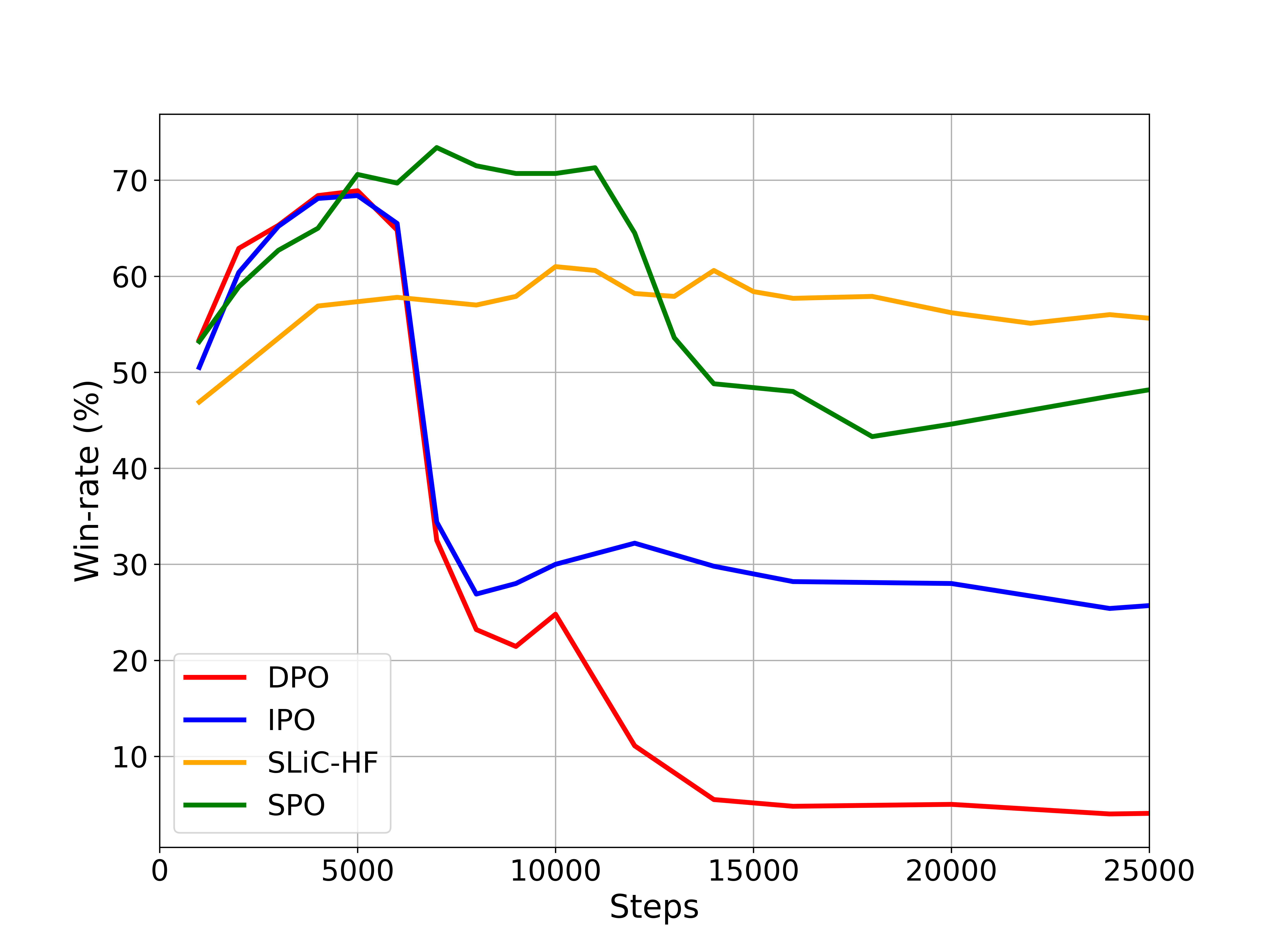
Figure 2: Win-rates of different alignment methods versus number of steps.

E.4 Compute resources

For the experiments of generating stories, we used a machine with four AMD Milan 7413 @ 2.65 GHz 128M cache L3 CPUs and a single NVidia A100SXM4 (40 GB memory) GPU. Training of each alignment algorithm was finished within 5 hours on the specified machine.

References

- [1] Paul F Christiano, Jan Leike, Tom Brown, Miljan Martic, Shane Legg, and Dario Amodei. Deep reinforcement learning from human preferences. Advances in neural information processing systems, 30, 2017.
- [2] Alec Radford, Karthik Narasimhan, Tim Salimans, Ilya Sutskever, et al. Improving language understanding by generative pre-training. 2018.
- [3] Prajit Ramachandran, Peter J Liu, and Quoc V Le. Unsupervised pretraining for sequence to sequence learning. arXiv preprint arXiv:1611.02683, 2016.
- [4] Long Ouyang, Jeffrey Wu, Xu Jiang, Diogo Almeida, Carroll Wainwright, Pamela Mishkin, Chong Zhang, Sandhini Agarwal, Katarina Slama, Alex Ray, et al. Training language models to follow instructions with human feedback. Advances in Neural Information Processing Systems, 35:27730–27744, 2022.
- [5] Rafael Rafailov, Archit Sharma, Eric Mitchell, Stefano Ermon, Christopher D Manning, and Chelsea Finn. Direct preference optimization: Your language model is secretly a reward model. arXiv preprint arXiv:2305.18290, 2023.
- [6] Afra Amini, Tim Vieira, and Ryan Cotterell. Direct preference optimization with an offset. arXiv e-prints, pages arXiv–2402, 2024.
- [7] Sayak Ray Chowdhury, Anush Kini, and Nagarajan Natarajan. Provably robust dpo: Aligning language models with noisy feedback. arXiv preprint arXiv:2403.00409, 2024.
- [8] Haoran Xu, Amr Sharaf, Yunmo Chen, Weiting Tan, Lingfeng Shen, Benjamin Van Durme, Kenton Murray, and Young Jin Kim. Contrastive preference optimization: Pushing the boundaries of llm performance in machine translation. arXiv preprint arXiv:2401.08417, 2024.
- [9] Yueqin Yin, Zhendong Wang, Yi Gu, Hai Huang, Weizhu Chen, and Mingyuan Zhou. Relative preference optimization: Enhancing llm alignment through contrasting responses across identical and diverse prompts. arXiv preprint arXiv:2402.10958, 2024.
- [10] Jing Xu, Andrew Lee, Sainbayar Sukhbaatar, and Jason Weston. Some things are more cringe than others: Preference optimization with the pairwise cringe loss. arXiv preprint arXiv:2312.16682, 2023.
- [11] Lewis Tunstall, Edward Beeching, Nathan Lambert, Nazneen Rajani, Kashif Rasul, Younes Belkada, Shengyi Huang, Leandro von Werra, Clémentine Fourrier, Nathan Habib, et al. Zephyr: Direct distillation of lm alignment. arXiv preprint arXiv:2310.16944, 2023.
- [12] Ralph Allan Bradley and Milton E Terry. Rank analysis of incomplete block designs: I. the method of paired comparisons. Biometrika, 39(3/4):324–345, 1952.
- [13] Mohammad Gheshlaghi Azar, Mark Rowland, Bilal Piot, Daniel Guo, Daniele Calandriello, Michal Valko, and Rémi Munos. A general theoretical paradigm to understand learning from human preferences. arXiv preprint arXiv:2310.12036, 2023.
- [14] R Duncan Luce. Individual choice behavior: A theoretical analysis. Courier Corporation, 2005.
- [15] Robin L Plackett. The analysis of permutations. Journal of the Royal Statistical Society Series C: Applied Statistics, 24(2):193–202, 1975.
- [16] John Schulman, Filip Wolski, Prafulla Dhariwal, Alec Radford, and Oleg Klimov. Proximal policy optimization algorithms. arXiv preprint arXiv:1707.06347, 2017.
- [17] Yao Zhao, Mikhail Khalman, Rishabh Joshi, Shashi Narayan, Mohammad Saleh, and Peter J Liu. Calibrating sequence likelihood improves conditional language generation. In The Eleventh International Conference on Learning Representations, 2022.
- [18] Ronen Eldan and Yuanzhi Li. Tinystories: How small can language models be and still speak coherent english? arXiv preprint arXiv:2305.07759, 2023.
- [19] Andrej Karpathy. llama2.c: Inference llama 2 in one file of pure c. https://github.com/karpathy/llama2.c, 2024. GitHub repository.
- [20] Karpathy. https://huggingface.co/karpathy/tinyllamas/commit/5c22d0a5f31b635f3e4bf8f2d4dd87363ae3a275, 2023.
- [21] Yao Zhao, Rishabh Joshi, Tianqi Liu, Misha Khalman, Mohammad Saleh, and Peter J Liu. Slic-hf: Sequence likelihood calibration with human feedback. arXiv preprint arXiv:2305.10425, 2023.
- [22] Josh Achiam, Steven Adler, Sandhini Agarwal, Lama Ahmad, Ilge Akkaya, Florencia Leoni Aleman, Diogo Almeida, Janko Altenschmidt, Sam Altman, Shyamal Anadkat, et al. Gpt-4 technical report. arXiv preprint arXiv:2303.08774, 2023.
- [23] Hugo Touvron, Louis Martin, Kevin Stone, Peter Albert, Amjad Almahairi, Yasmine Babaei, Nikolay Bashlykov, Soumya Batra, Prajjwal Bhargava, Shruti Bhosale, et al. Llama 2: Open foundation and fine-tuned chat models. arXiv preprint arXiv:2307.09288, 2023.
- [24] Hanze Dong, Wei Xiong, Deepanshu Goyal, Rui Pan, Shizhe Diao, Jipeng Zhang, Kashun Shum, and Tong Zhang. Raft: Reward ranked finetuning for generative foundation model alignment. arXiv preprint arXiv:2304.06767, 2023.
- [25] Tianjun Zhang, Fangchen Liu, Justin Wong, Pieter Abbeel, and Joseph E Gonzalez. The wisdom of hindsight makes language models better instruction followers. arXiv preprint arXiv:2302.05206, 2023.
- [26] Caglar Gulcehre, Tom Le Paine, Srivatsan Srinivasan, Ksenia Konyushkova, Lotte Weerts, Abhishek Sharma, Aditya Siddhant, Alex Ahern, Miaosen Wang, Chenjie Gu, et al. Reinforced self-training (rest) for language modeling. arXiv preprint arXiv:2308.08998, 2023.
- [27] Rémi Munos, Michal Valko, Daniele Calandriello, Mohammad Gheshlaghi Azar, Mark Rowland, Zhaohan Daniel Guo, Yunhao Tang, Matthieu Geist, Thomas Mesnard, Andrea Michi, et al. Nash learning from human feedback. arXiv preprint arXiv:2312.00886, 2023.
- [28] Corby Rosset, Ching-An Cheng, Arindam Mitra, Michael Santacroce, Ahmed Awadallah, and Tengyang Xie. Direct nash optimization: Teaching language models to self-improve with general preferences. arXiv preprint arXiv:2404.03715, 2024.
- [29] Gokul Swamy, Christoph Dann, Rahul Kidambi, Zhiwei Steven Wu, and Alekh Agarwal. A minimaximalist approach to reinforcement learning from human feedback. arXiv preprint arXiv:2401.04056, 2024.
- [30] Yoav Freund and Robert E Schapire. A decision-theoretic generalization of on-line learning and an application to boosting. Journal of computer and system sciences, 55(1):119–139, 1997.
- [31] Rafael Rafailov, Joey Hejna, Ryan Park, and Chelsea Finn. From r to q*: Your language model is secretly a q-function. arXiv preprint arXiv:2404.12358, 2024.
- [32] Tianqi Liu, Yao Zhao, Rishabh Joshi, Misha Khalman, Mohammad Saleh, Peter J Liu, and Jialu Liu. Statistical rejection sampling improves preference optimization. In The Twelfth International Conference on Learning Representations, 2023.