Federated Graph Learning for EV Charging Demand Forecasting with Personalization
Against Cyberattacks
Abstract
Mitigating cybersecurity risk in electric vehicle (EV) charging demand forecasting plays a crucial role in the safe operation of collective EV chargings, the stability of the power grid, and the cost-effective infrastructure expansion. However, existing methods either suffer from the data privacy issue and the susceptibility to cyberattacks or fail to consider the spatial correlation among different stations. To address these challenges, a federated graph learning approach involving multiple charging stations is proposed to collaboratively train a more generalized deep learning model for demand forecasting while capturing spatial correlations among various stations and enhancing robustness against potential attacks. Firstly, for better model performance, a Graph Neural Network (GNN) model is leveraged to characterize the geographic correlation among different charging stations in a federated manner. Secondly, to ensure robustness and deal with the data heterogeneity in a federated setting, a message passing that utilizes a global attention mechanism to aggregate personalized models for each client is proposed. Thirdly, by concerning cyberattacks, a special credit-based function is designed to mitigate potential threats from malicious clients or unwanted attacks. Extensive experiments on a public EV charging dataset are conducted using various deep learning techniques and federated learning methods to demonstrate the prediction accuracy and robustness of the proposed approach.
Index Terms:
EV Charging demand forecast, cybersecurity, personalized federated learning, graph neural networks, malicious attack.I Introduction
The growing adoption of electric vehicles (EVs) by both individuals and businesses has raised concerns about the potential strain on the grid and charging infrastructure. Accurate demand forecasts are essential for sustainable operations of the electric vehicle - charging station - power grid ecosystem, which, in turn, facilitates the electrification and decarbonization of the transportation sector [1]. There has been extensive research conducted on EV charging demand forecasting by collecting a large number of EV charging information to train a deep learning model for better prediction performance in a centralized way [2, 3, 4, 5]. However, training a deep model usually acquires IoT devices over a communication system embedded within an EV charging station for information exchange, which is susceptible to cyberattacks such as False Data Injection (FDI) [6]. Adversary robust methods or anomaly detection methods should be investigated against these cyberattacks [7][8]. Moreover, data collected from different stations have privacy concerns which may reveal consumers’ privacy, e.g., traveling routes, home and office addresses, payment information, individual preferences, etc., opening doors for exploiting the EV charging infrastructure through various vulnerable components in the cyber-layer if they are sent to a central server. Therefore, concerning privacy and cyberattack issues, it is essential to find a safe and privacy-preserving way to train the charging demand forecasting model that can leverage the charging data in different stations without violating data privacy.
It is widely acknowledged that Federated learning (FL) can harness the information among different clients by sharing the model rather than the data, which provides a secure and private way for different stations/operators to collaboratively train EV charging demand forecasting models [9]. FL can also protect privacy against several types of cyberattacks at the data level [10], including denial of service (DoS), structured query language (SQL), and man-in-the-middle. However, it still faces the risk of malicious attacks on the local models when transmitting to the server. In such a case, the commonly used “averaging” becomes susceptible to arbitrary manipulation even if just one local model is compromised [11]. Typical Byzantine robust methods classify the malicious by clustering, or geometric median, which is effective in malicious attacks [12]. Nevertheless, these methods train a shared model for all the clients, which can degrade the performance of some or all participants because the data in different stations are not independent and identically distributed (non-i.i.d). Therefore, proposing the personalized federated learning framework is of great importance to EV charging stations, considering their heterogeneous data distribution. Many personalized techniques have been proposed to address the data heterogeneity issue, including local tuning, model interpolation, clustering, and multi-task learning [13, 14, 15, 16]. However, most personalized methods incorporate “averaging” aggregation in the server, which is quite vulnerable to threat models.
In the EV demand forecasting area, few papers have adopted the federated learning technique to improve their forecasting performance. In [17], vanilla FedAvg is first applied to the energy demand forecasting for EV network, while federated cluster learning is further proposed to improve the training efficiency and personalized performance. Although clustering helps to improve personalized performance, the inter-cluster feature is not learned with the framework, which deteriorates the generalized performance of the global model in each cluster. Similarly, in [18], a blockchain-based hierarchical federated learning is proposed for EV charging demand forecasting, while the clustering method is used to get a personalized model for each cluster. Nevertheless, the cybersecurity and the correlated relationship between and inside the clusters are not considered. To protect data privacy against different kinds of cyberattacks for EV energy demanding forecasting, a secure FL is proposed in [19], where a double authentication process is designed to avoid the attacked model from the client or server. Despite being effective against the cyberattack, the global model is aggregated by ”averaging”, which fails to generate personalized models for each client.
Furthermore, unlike traditional fuel stations that typically adhere to uniform consumption patterns and demand trends, EV charging stations can exhibit substantial variations influenced by factors such as geographic location, infrastructure availability, charging speed, and user preferences. Given the multifaceted nature of these factors impacting the behavior of EV charging stations, it becomes increasingly imperative to consider not only the temporal aspects within an individual station but also the broader context of data interconnection and interoperability, as elucidated in references [20, 21, 22, 23, 24]. In terms of capturing spatial information, Graph neural networks (GNNs) are a promising paradigm that has been applied to capture deep patterns and handle dependencies among time series across different problems in different fields, including traffic forecasting [25], situation recognition [26]. Currently, few GNN-based methods have been applied to the EV charging demand forecasting. [21, 20] integrates different EV charging station data to improve the generalization using temporal GNN that incorporates both spatial and temporal features into the forecasting process. Recent research has generally revealed that many machine learning models suffer from security vulnerabilities; the same applies to GNNs. Therefore, it is critical to design an intrinsically secure message-passing mechanism for graph-structured data. In [27], AirGNN denoises the hidden features in neural network layers caused by the adversarial perturbation using the graph structural information. More importantly, robustness is another concern for federated learning, where malicious attacks could happen during the transmission or aggregation process. A federated spatio-temporal model CNFGNN is proposed in [28], which can effectively model the complex spatio-temporal dependencies. However, CNFGNN does not take into account malicious attacks and the robustness of the algorithm, leaving room for further exploration in this critical aspect of model security to ensure that the model can maintain the robustness under attack while protecting the privacy and security of user data.
Considering the challenges of data privacy, cybersecurity, and the correlations among stations, this paper proposes a robust federated graph learning method with personalization. The core idea is to leverage the correlated information among limited stations/operators while avoiding malicious attacks and alleviating the influence brought by data heterogeneity. Specifically, operators with similar data distribution are encouraged to collaborate more, while the Byzantine robustness for each operator is guaranteed based on an attention-inducing mechanism. In addition, the correlated information is captured by the GNN. Contributions to the paper are as follows:
-
1.
Propose a federated graph learning framework for EV charging demand forecasting with advanced deep learning methods. It enables the stations to collaboratively train models that capture the common spatial-temporal patterns as well as the correlations between the client’s model and thus enhance the overall forecasting performance while protecting the data privacy of the stations.
-
2.
Design a message passing aggregation method based on the similarity among the forecasting model of stations to encourage the stations with similar charging data distribution to collaborate more and train a personalized forecasting model tailored for each station. The convergence of the proposed method is provided mathematically.
-
3.
Propose a credit-based method to ensure the similarity among different stations can be captured with varied training models while guaranteeing robustness to unwanted threats models during federated aggregation. The proposed mechanism allows a quantitative description of the relationship between the different charging station operators, where the similarity can be tuned adaptively with the guiding of the credit that one station has put on the rest of the stations.
The rest of this paper is organized as follows: Section II formulates the problem to be studied; Section III provides the overall framework of the proposed personalized federated graph learning and analyzes the convergence and robustness of the method; Section IV conducts comparative experiments and analysis on the Palo Alto dataset; Section V draws the conclusions.
II Problem Formulation
II-A EV Charging Demand Forecasting
The goal is to predict the future EV charging demand of charging stations in an area. We use historical demand from charging stations and calendar variables as input features. Specifically, the calendar variables refer to hour of the day, day of the week, day of the month, day of the year, month of the year, and the year. The demand observation of -th charging station at time step is denoted as . The corresponding calendar variables of the charging station are denoted as . For convenience, we use denotes , and denotes . The demand observation series of time steps of -th station is denoted as . Similarly, the demand forecast series of time steps of -th station is denoted by . Notably, the quantile loss is used for training a probabilistic forecasting model. Quantile regression models estimate the conditional quantile of the target distribution , given the quantile ,i.e., minimizing the quantile loss or tilted loss:
| (1) |
where is the predicted value, and . In this paper, the multi-output quantile regression neural network (MQNN) is adopted to improve the computation efficiency by training a model that fits all the quantiles. Suppose is the number of quantiles, then the matrix will be the output of the MQNN of station ; MQNN will find the model that minimizes the summed quantile loss of different quantiles, i.e., .
Additionally, to simultaneously consider the spatial-temporal correlations and enhance the generalization of our model, we go a step further by incorporating the correlation between charging station demands. This is achieved through graph neural networks and attention-based message passing. Specifically, we have constructed two graphs to capture both spatial-temporal correlations and the model similarity among stations. The first spatial graph, , is designed to capture the spatial and temporal correlations, where represents the set of stations, denotes the edges, and serves as the weighted adjacency matrix, which is defined based on the distance. To be specifically, if the distance between stations , is below a certain threshold, , which means , otherwise , . The other graph is designed to capture the similarity of the forecasting model in different stations, which is denoted as the model similarity graph, . encompasses the set of station’s models, signifies the edges, and serves as the weighted adjacency matrix, which is calculated based on the similarity between the models. In this study, we leverage both spatial connections and similarities among station’s models to encapsulate the relationships between charging stations. Consequently, the EV charging demand forecasting can be further represented as:
| (2) |
| (3) |
II-B New FL for Charging Demand Forecasting
Due to privacy concerns, the historical charging data or model in different stations will not be shared with other stations directly. To realize (3) without sharing the embedding between stations, FL with a central server is applied. Commonly used FL, such as FedAvg, aims to find a common model for all the clients (refer to stations in this paper) by solving the following optimization problem:
| (4) |
where , are the loss function of the forecasting model and the dataset of client ; is the weight attributed to client based on clients’ dataset, and represents the total clients in the federated learning.
In FL framework, the server will first send a global model to all participated clients, and each client will update their model based on the local data; after that, clients will upload their model or gradient to the server, while the server will aggregate a new global model with the collected model/gradient and use it as the initial model of the next round [9].
Due to the difference between the habits of the EV owners and the spatial distribution of the charging stations, the charging demand data in different stations vary. In such a case, we argue that an identical model for all stations may not be suitable, and personalized models by which both the common features among stations and individual features can be learned are required. A typical way to obtain a personalized model is to update the local model with local data while using the global model as a penalized term to ensure the global information is learned by the local model [29], i.e.
| (5) |
where is the penalization coefficient. Such a method can get an effective personalized model, while the global model is obtained using ”averaging” aggregation, which is vulnerable to malicious attacks. Once one of the clients sends the false model information to the server, the aggregated global model will be poisoned, and thus lead to a worse performance of the local model. Therefore, to improve the robustness of the global model to work against malicious model attacks, a new aggregation rule is required, and (5) can be rewritten as:
| (6) |
where ; is the desired function to generate the weight for a more robust global aggregation. In this paper, we denote an attention-based function that is calculated based on the similarity between the and , and a credit parameter that represents the credit of station has put on the rest of the stations. In such an aggregation rule, the poisoned local model will be attributed to small weights, and thus cause a mere effect on the global model. As indicated in (6), the server will aggregate different global models for different clients to work against the malicious model attack. Additionally, each station/client will optimize:
| (7) |
which will force the client with similar data distribution to collaborate more, i.e., client will be closer to the one that is similar to it since more weight is attributed to these clients. Note that there is a credit parameter to control . In addition, the model aggregation (message passing) with specific weights is implemented in the server.
III Proposed Personalized Federated Graph Learning Method
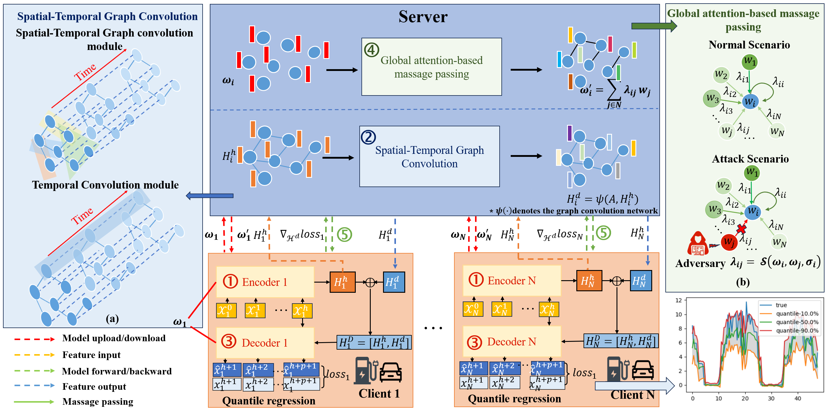
The framework of the proposed method is illustrated in Fig. 1, which involves the following steps, each marked with a corresponding stage number in the figure for clarity:
-
1.
Encoder Feature Extraction: Each EV charging station uses a 1D Conv Encoder for feature extraction. The extracted features are then sent to the central server.
-
2.
Spatial-Temporal Graph Convolution: The server employs spatial-temporal graph convolution networks to model spatial-temporal dependencies, creating the spatial-temporal feature (i.e., in Fig. 1).
-
3.
Decoder Forecasting: The output features of spatial-temporal graph convolution networks are downloaded by each client and then combined with the initial feature , forming as inputs to Forecasting module which consists of 1D Convs and Linear networks.
-
4.
Global Attention-based Message Passing: The local model parameters are uploaded to the server. The server will aggregate different global models for different clients based on the model similarities and spatial relationships among clients, which achieves message passing between different clients. After that, the server will seed the aggregated global models to corresponding clients for local training.
-
5.
Local training: Each client will update the local model with the received global model and local data by solving problem (7).
In the following, we will describe each of the above steps in detail, where 1, 2, and 3 correspond to subsection A, and 4 and 5 correspond to subsection B. Additionally, we analyzed the convergence and robustness of personalized federated learning.
III-A Spatial-Temporal Graph Convolution Networks
We first apply a 1D Conv layer to extract high-level features from the input EV charging time-series data. These features are then combined and processed using Spatial-temporal graph convolution networks. Spatial-temporal graph convolution networks are used to capture spatial and temporal dependencies [30], which consist of a spatial-temporal convolution module and a temporal convolution module, as described in Fig. 1(a). The former aggregates spatial information from the neighborhood, while the latter uses convolution neural networks along the temporal dimension. In this paper, multiple spatial-temporal graph convolution networks are stacked to extract dynamic spatial-temporal correlations. We now introduce the spatial-temporal attention mechanism and spatial-temporal graph convolution in the GNN layer.
Spatial-Temporal Attention Mechanism:
1) Spatial attention:
| (8) |
| (9) |
where is the input of the -th spatial-temporal graph convolution networks. and denote the input data embedding dimension and input feature dimension of the -th layer. When , . , , , are learnable parameters and sigmoid is used as the activation function. captures the spatial correlation strength between station and station . When conducting the graph convolutions, we will accompany the weighted adjacency matrix with the spatial attention matrix to dynamically adjust the impacting weights between stations.
2) Temporal attention:
| (10) |
| (11) |
where , , , are learnable parameters. represents the level of temporal dependencies between time and . We then apply the normalized temporal attention matrix directly to the input and get .
Spatial-Temporal Graph Convolution:
First, the input undergoes graph convolution[31] in the spatial dimension, aimed at capturing neighboring information for each station. After the graph convolution operations, we incorporate a standard convolution layer in the temporal dimension. The temporal convolution operations can update the station’s embedding by involving the information at the neighboring time slice, represented as:
| (12) |
In the graph convolution operation, denotes graph convolution, and denotes the graph kernel. The process of graph convolution can be represented as , where . stands for the normalized Laplace matrix, which can be calculated as follows, , where denotes the maximum eigenvalue of . , where denotes the graph degree matrix. To dynamically adjust the correlations between stations, we accompany with the spatial attention matrix , then obtain , where is the Hadamard product. Hence, In the temporal convolution operation, denotes a standard convolution, is the parameter of the temporal dimension convolution kernel, and the activation function is ReLU. Then the final output spatial-temporal feature and will be concatenated together and input to the Decoder to forecast the multi-quantiles output.
III-B Personalized Federated Learning
In the proposed federated graph learning framework, all clients solve the optimization problem (6) in a federated manner to protect data privacy while obtaining personalized models. Specifically, each client will update the local model for iterations to find an inexact solution of (7), and then send the local model to the server for aggregation. The server will aggregate different global models for different clients once it receives the local models from clients and then distributes the global models to corresponding clients for local training. To work against malicious model attacks from clients during the global model aggregation, the aggregation weights of the local models are calculated based on the similarity among models. Therefore, the malicious model will be considered not similar to the normal one and thus attribute small weights during aggregation. Such aggregation method is denoted as message passing, in which clients share messages that combine information from their neighboring clients’ models and their own model. The global model aggregation process for client can be modeled as:
| (13) | ||||
| (14) | ||||
| (15) |
where represents the model of -th client at communication rounds, and ; is an attention mechanism-based function that measures the difference/similarity level between and , which decrease monotonically and it satisfies: , and
| (16) |
Note that have the same function as in (6). In addition, when is below a threshold (the corresponding client can be considered as a malicious one), its value will be set to zero. There are many functions that can satisfy . In this paper, we chose , where is considered as a credit parameter that client put on other clients. Moreover, to leverage the spatial relationship among different stations, the similarity value is reweighted with the spatial graph weighted adjacency matrix , i.e.,
| (17) |
where is a constant to balance and , which is called channel weight. Note that the client with will be deleted during the aggregation to guarantee the robustness of the global model. For better understanding, the proposed personalized federated learning algorithm is summarized in Algorithm 1.
III-C Convergence Analysis
For convenience of convergence analysis, the following assumptions are made.
Assumption 1.
Function is L-smooth for , i.e., there exists a constant , for all , .
Assumption 2.
The gradient of is bounded, i.e., for every .
Assumption 3.
The difference between the global model and local model of the client is bounded for , i.e., there exists a constant such that for every , where is the local learning rate.
Theorem 1.
Proof.
See appendix A ∎
Theorem 1 indicates that the proposed algorithm will help the model in each client converge to a stable point, while the convergence speed is determined by the local epochs , communication rounds , and the , .
III-D Robust Analysis Against Cyberattacks
In this paper, the robustness of the personalized model is guaranteed by designing the attention-based function , and it is chosen as , where is considered as a credit parameter that client put on other clients. Intuitively, large means client gives high credit to the other clients and believes that the data distribution in other clients is similar to itself, whereas small means conversely. If one of the local model is poisoned, then its similarity value to model will be small. Thus, the effect of the poisoned model to the global model of client will be trivial. In this paper, we assume that there is at least one client that owns a similar data distribution to client , and we set the similarity value of client that is most similar to client as , such that is determined and will be determined adaptively, namely:
| (18) |
and therefore . Based on (18), the normalized vector helps to work against the scaling attack, and then the attention-based function could still work even when the dimension of , and are high, which is often the case for deep neural networks. Based on the above analysis, we argue that the robustness of the global model for different clients can be guaranteed with the designed function .
IV Case Studies
We conducted case studies on the Palo Alto dataset, which was collected from January 1, 2018, to January 1, 2020, from the city of Palo Alto [32]. It consists of 8 EV charging stations. For the data pre-processing, the EV charging transaction is recorded as events, which includes the electricity charging demand (kWh) and the charging start time and end time. Hence, considering the time-varying and periodicity of EV charging events, each day is divided into 48 periods. The original charging session records are then discretized into 25,9415 pieces of data, aggregated over 30-minute intervals for each specific station. Hence, each station has 34,993 data entries.
IV-A Baseline Approaches
We compare our Personalized Federated Graph Learning framework (denoted as PFGL) with the following 6 benchmark methods:
-
1.
Purely Local Framework (No_FL), where each client only applies its own historical charging demand data to train a model (CNN-based Encoder-Decoder) without communication and uses it for demand forecasting.
-
2.
LSTM-FedAvg[33], which is a federated model based on LSTM. LSTM is utilized to obtain the features, and FedAvg is used to obtain a global model.
-
3.
LSTM-PFL,which is a federated model based on LSTM. Personalized federated learning is used to obtain personalized models.
-
4.
LSTM-CNN-FedAvg, which is a federated model based on LSTM. CNN is utilized to convolution client features in the server, and FedAvg is used to obtain a global model.
-
5.
LSTM-CNN-PFL, which is a federated model based on LSTM. CNN is utilized to convolution client features in the server, personalized federated learning is used to obtain personalized models.
-
6.
CNFGNN [28], which is a federated spatio-temporal model based on GNNs. CNFGNN separates temporal and spatial dynamics during aggregation, and FedAvg is used to obtain a global model.
IV-B Experimental Setups
IV-B1 Implementation Details
In the experiment, the single step, as well as the multi-step technique, are used (prediction steps are set to 1 and 6) for comparisons. The batch size for all models is 32, and the learning rates of No_FL, LSTM-CNN-FedAvg, LSTM-CNN-PFL, CNFGNN, and PFGL are set to 0.0005, while LSTM-FedAvg, LSTM-PFL are set to 0.001. For time series prediction methods, we employ a sliding window of size 32. For No_FL, LSTM-CNN-FedAvg and LSTM-CNN-PFL, the kernel size of 1D Conv modules are both 64 and the Linear networks have 64 hidden units. There exists 2 layer LSTM module in LSTM-FedAvg, LSTM-CNN-FedAvg and LSTM-CNN-PFL, the hidden size of each layer are 32 and 64, respectively. PFGL employs Chebyshev polynomial terms () and has a temporal convolution module with a kernel size of 3. Additionally, its 1D Conv Encoder and Decoder have a kernel size of 64 to capture long temporal dependencies. PFGL includes 2 spatial-temporal graph convolution networks, where the hidden units of the graph convolution module and the temporal convolution module are set to 64. For and , in single-step prediction: =0.8, =0.8. In 6-step prediction: =0.9, =0.9. In addition, we set to to comprehensively assess the model’s capability in providing probabilistic predictions across different levels of confidence intervals. To ensure model generalization and mitigate overfitting, we divided the dataset into a training set (60%), a validation set (20%), and a testing set (20%). We perform 100 communication rounds and select the model with minimal global validation loss as the final model.
IV-B2 Evaluation Metrics
We evaluate the performance via the quantile loss (QS), as well as two common measures of Quantile Regression, Mean Interval Length (MIL) and Interval Coverage Percentage (ICP), as summarized in Table I, where, is the predicted quantile for observation at timestamp and , is a higher quantile than . For both measures, we define the prediction interval as the interval between the and the . And is the test dataset size and is the index value of the test instance. The ICP should be close to 0.9-0.1=0.8, while the MIL should be as small as possible. Among models with the same ICP, the one that yields the lowest MIL is preferred.
IV-C Performance without Malicious Attacks
The performance of the proposed method is compared with the result of the baseline. The QS, MIL, and ICP of different methods are shown in Table II, III, and IV respectively. The “improved rate” represents the percentage of nodes whose results are better than those of the No_FL.
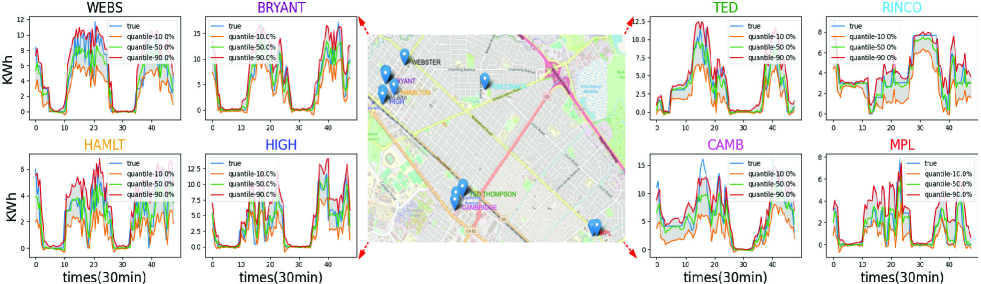
In steps 1 and 6, the forecasting results of QS loss show that PFGL outperforms other baselines in 5/8 and 6/8 stations respectively, with the average QS loss value being the best. For MIL, PFGL surpasses baselines for 6/8 stations in steps 6 forecasting results, with the mean MIL values also indicating superior performance. In the case of ICP, PFGL outperforms other baselines for step 1 forecasting results in 5/8 stations, with the mean ICP values of steps 1 and 6 indicating superior performance. These results illustrate the improvement offered by our proposed model, particularly evident in the long-term forecasting accuracy of QS loss. This highlights the effectiveness of employing a personal federated aggregation approach to improve prediction accuracy. For demonstration, the 6-step ahead prediction results of the PFGL for different stations are drawn, as shown in Fig. 2. Furthermore, the comparison between baseline LSTM-FedAvg and LSTM-CNN-FedAvg (LSTM-PFL with LSTM-CNN-PFL) reveals a decrease in QS loss, indicating that the convolution operation efficiently enhances forecasting accuracy. This also suggests that when information is aggregated after passing through a CNN or GNN, it is more effective than direct aggregation. Additionally, most of the results of LSTM-PFL outperform LSTM-FedAvg, highlighting the efficiency of the PFL framework. When comparing PFGL to CFNGNN, two federated learning frameworks based on graph neural networks, PFGL achieves mostly superior outcomes. This outcome highlights PFGL’s ability to model the temporal trajectory of multivariate time series. Furthermore, it demonstrates PFGL’s capacity to capture spatial and temporal correlations simultaneously, ultimately enhancing prediction accuracy.
| Method | WEBS | HIGH | TED | MPL | CAMB | BRYANT | HAMLT | RINCO | Avg | Improved rate | |
|---|---|---|---|---|---|---|---|---|---|---|---|
| Step 1 | No_FL | 0.9973 | 1.1415 | 0.8761 | 0.7271 | 1.1348 | 1.0764 | 0.7285 | 0.6035 | 0.9107 | 0% |
| LSTM-FedAvg | 0.9842 | 1.0976 | 0.9069 | 0.7268 | 1.1435 | 1.0472 | 0.7699 | 0.6603 | 0.9171 | 50% | |
| LSTM-CNN-FedAvg | 0.967 | 1.0862 | 0.8445 | 0.7131 | 1.1492 | 1.011 | 0.701 | 0.5859 | 0.8823 | 87.5% | |
| LSTM-PFL | 0.9706 | 1.0907 | 0.8604 | 0.7196 | 1.1055 | 1.033 | 0.7244 | 0.6117 | 0.8895 | 87.5% | |
| LSTM-CNN-PFL | 0.984 | 1.0697 | 0.844 | 0.7129 | 1.1502 | 1.0159 | 0.7044 | 0.5723 | 0.8817 | 87.5% | |
| CNFGNN | 0.9251 | 1.0634 | 0.8406 | 0.6934 | 1.1053 | 1.0228 | 0.6939 | 0.5736 | 0.8648 | 100% | |
| PFGL | 0.9289 | 1.0561 | 0.8445 | 0.6942 | 1.091 | 1.0083 | 0.6938 | 0.5531 | 0.8587 | 100% | |
| Step 6 | No_FL | 1.6377 | 1.8104 | 1.5343 | 1.2219 | 1.8841 | 1.8705 | 1.1031 | 1.1208 | 1.5228 | 0% |
| LSTM-FedAvg | 1.5075 | 1.6605 | 1.5281 | 1.214 | 1.8111 | 1.7175 | 1.1534 | 1.2843 | 1.4846 | 75% | |
| LSTM-CNN-FedAvg | 1.4921 | 1.6805 | 1.416 | 1.1844 | 1.861 | 1.6717 | 1.0111 | 1.0968 | 1.4267 | 100% | |
| LSTM-PFL | 1.5107 | 1.6504 | 1.4995 | 1.2037 | 1.7949 | 1.6674 | 1.1186 | 1.225 | 1.4588 | 75% | |
| LSTM-CNN-PFL | 1.4756 | 1.6808 | 1.4452 | 1.1794 | 1.839 | 1.6718 | 1.0113 | 1.0986 | 1.4252 | 100% | |
| CNFGNN | 1.3489 | 1.5789 | 1.3559 | 1.1612 | 1.7699 | 1.5729 | 0.9532 | 1.0793 | 1.3525 | 100% | |
| PFGL | 1.3813 | 1.6095 | 1.3248 | 1.1277 | 1.6425 | 1.561 | 0.9469 | 1.034 | 1.3285 | 100% |
| Method | WEBS | HIGH | TED | MPL | CAMB | BRYANT | HAMLT | RINCO | Avg | Improved rate | |
|---|---|---|---|---|---|---|---|---|---|---|---|
| Step 1 | No_FL | 3.2895 | 3.3887 | 2.6677 | 2.2182 | 3.4256 | 3.4951 | 2.5997 | 1.7068 | 2.8489 | 0% |
| LSTM-FedAvg | 3.3085 | 3.5621 | 2.8975 | 2.1461 | 3.6088 | 4.1508 | 1.9084 | 1.9912 | 2.9467 | 25% | |
| LSTM-CNN-FedAvg | 3.1142 | 3.1183 | 2.4359 | 2.0102 | 3.4061 | 3.353 | 2.426 | 1.719 | 2.6978 | 87.5% | |
| LSTM-PFL | 3.1057 | 3.5875 | 2.7625 | 2.0527 | 3.488 | 3.7674 | 2.0447 | 1.7433 | 2.819 | 37.5% | |
| LSTM-CNN-PFL | 2.955 | 3.2347 | 2.4363 | 2.0022 | 3.3019 | 3.3621 | 2.3433 | 1.6445 | 2.66 | 100% | |
| CNFGNN | 3.1372 | 3.1707 | 2.4386 | 2.0509 | 3.5784 | 3.3498 | 2.2508 | 1.7596 | 2.717 | 75% | |
| PFGL | 3.1147 | 3.0815 | 2.4979 | 2.0429 | 3.5923 | 3.3165 | 2.3058 | 1.6435 | 2.6999 | 87.5% | |
| Step 6 | No_FL | 4.8827 | 5.453 | 4.2709 | 4.1653 | 5.4922 | 6.2315 | 3.708 | 3.484 | 4.711 | 0% |
| LSTM-FedAvg | 5.014 | 5.3843 | 4.4358 | 3.4362 | 5.3279 | 6.7106 | 2.9766 | 3.1284 | 4.5517 | 63.3% | |
| LSTM-CNN-FedAvg | 4.2879 | 4.7923 | 4.1441 | 3.7645 | 4.8621 | 5.6288 | 3.1034 | 3.3035 | 4.2358 | 100% | |
| LSTM-PFL | 4.892 | 5.2963 | 4.3127 | 3.4221 | 5.1952 | 6.239 | 3.0354 | 3.092 | 4.4356 | 63.3% | |
| LSTM-CNN-PFL | 4.4348 | 4.7678 | 3.8686 | 3.6398 | 4.9492 | 5.3042 | 3.0571 | 3.1986 | 4.1525 | 100% | |
| CNFGNN | 4.2927 | 4.5791 | 3.7782 | 3.7633 | 4.5811 | 5.1661 | 3.0256 | 3.3389 | 4.0656 | 100% | |
| PFGL | 4.2209 | 4.5749 | 3.5493 | 3.6281 | 4.5568 | 5.0724 | 2.9645 | 3.1659 | 3.9666 | 100% |
| Model | Method | WEBS | HIGH | TED | MPL | CAMB | BRYANT | HAMLT | RINCO | Avg | Improved rate |
|---|---|---|---|---|---|---|---|---|---|---|---|
| Step 1 | No_FL | 0.8089 | 0.7804 | 0.7365 | 0.8007 | 0.7618 | 0.8219 | 0.8264 | 0.8066 | 0.7929 | 0% |
| LSTM-FedAvg | 0.8378 | 0.8468 | 0.8448 | 0.8218 | 0.8111 | 0.8995 | 0.464 | 0.8283 | 0.7942 | 25% | |
| LSTM-CNN-FedAvg | 0.8312 | 0.8145 | 0.6424 | 0.7203 | 0.7672 | 0.7335 | 0.8362 | 0.8111 | 0.7696 | 25% | |
| LSTM-PFL | 0.5825 | 0.8483 | 0.846 | 0.7287 | 0.8132 | 0.8807 | 0.804 | 0.8237 | 0.7909 | 37.5% | |
| LSTM-CNN-PFL | 0.8138 | 0.8035 | 0.8035 | 0.6792 | 0.7057 | 0.7452 | 0.8483 | 0.8019 | 0.779 | 37.5% | |
| CNFGNN | 0.803 | 0.7694 | 0.7515 | 0.7655 | 0.7846 | 0.7877 | 0.7886 | 0.7538 | 0.7755 | 62.5% | |
| PFGL | 0.7887 | 0.7962 | 0.8258 | 0.773 | 0.7976 | 0.798 | 0.8279 | 0.7977 | 0.8006 | 75% | |
| Step 6 | No_FL | 0.7353 | 0.7713 | 0.7488 | 0.7734 | 0.7419 | 0.7902 | 0.7481 | 0.7592 | 0.7585 | 0% |
| LSTM-FedAvg | 0.5818 | 0.789 | 0.7603 | 0.4764 | 0.7955 | 0.7921 | 0.4762 | 0.7095 | 0.6726 | 50% | |
| LSTM-CNN-FedAvg | 0.7194 | 0.7039 | 0.7642 | 0.7449 | 0.7372 | 0.7757 | 0.7631 | 0.7555 | 0.7455 | 25% | |
| LSTM-PFL | 0.5702 | 0.8309 | 0.7679 | 0.4802 | 0.7899 | 0.8676 | 0.4973 | 0.7269 | 0.691 | 25% | |
| LSTM-CNN-PFL | 0.7749 | 0.7466 | 0.7644 | 0.7616 | 0.743 | 0.8038 | 0.7376 | 0.7111 | 0.7554 | 50% | |
| CNFGNN | 0.7404 | 0.7411 | 0.7355 | 0.7563 | 0.7021 | 0.7206 | 0.764 | 0.7521 | 0.739 | 25% | |
| PFGL | 0.7634 | 0.7268 | 0.766 | 0.7965 | 0.7565 | 0.7878 | 0.77 | 0.7542 | 0.7652 | 62.5% |
IV-D Performance under Malicious Attacks
In the proposed PFL, each client will be given a personalized aggregated model by attributing different weights to the clients’ model, where the weights are calculated based on the similarity between the target client and other clients. In such a manner, clients with parameters that differ much from the target client will be attributed to less weight when performing aggregation. Naturally, when a malicious participant sends an arbitrary local model, the local model will be attributed to small or even near zero weight when it is used to aggregate the global model of another client. To testify the proposed method under false data injection attack, one of the clients is selected to send manipulated models, while three kinds of manipulating methods including parameter flipping, scaling, and Gaussian noise are carried out to generate the threat model, as indicated in (19);
| (19) |
| Model | Malicious nodes | LSTM-FedAvg | LSTM-CNN-FedAvg | LSTM-PFL | LSTM-CNN-PFL | CNFGNN | PFGL |
|---|---|---|---|---|---|---|---|
| Local | 0 | 1.4846 | 1.4267 | 1.4588 | 1.4252 | 1.3525 | 1.3285 |
| Flipping | 1 | 2.3646 | 1.4262 | 1.4351 | 1.4262 | 1.351 | 1.331 |
| 4 | 4.2189 | 1.4262 | 1.4775 | 1.4262 | 1.3562 | 1.3251 | |
| 8 | 4.4764 | 1.4262 | 1.4382 | 1.4262 | 1.3562 | 1.3281 | |
| Scaling | 1 | 1.4867 | 1.4275 | 1.437 | 1.451 | 1.3562 | 1.3405 |
| 4 | 1.5302 | 1.4275 | 1.4268 | 1.451 | 1.3561 | 1.3378 | |
| 8 | 1.5519 | 1.4275 | 1.4226 | 1.451 | 1.3378 | 1.3316 | |
| Gaussian noise | 1 | 1.4907 | 1.4225 | 1.4383 | 1.4225 | 1.3668 | 1.3405 |
| 4 | 1.5302 | 1.424 | 1.446 | 1.424 | 2.4749 | 1.3415 | |
| 8 | 1.5519 | 1.4263 | 1.4352 | 1.4263 | 1.3601 | 1.3292 |
Since the goal of the task is to forecast the demand for EV, we use the average QS loss as the metric to evaluate its effectiveness of the proposed model to counteract malicious clients. The attack results of the baselines and the proposed PFGL are shown in Table V. It is seen that the average quantile loss for 8 stations under three kinds of attack increased drastically when it is trained using averaging aggregation (LSTM-FedAvg case), indicating that LSTM-FedAvg cannot bear attacks from even a single client. The proposed PFGL, however, can work against three kinds of attacks and still get a lower quantile loss than that of the solely local training method. In order to demonstrate the robustness of the proposed PFL, the proportion of malicious clients is increased, specifically for 1/8 to 8/8. When the portion of the malicious increases, the average QS of baseline increases sharply, whereas that of the proposed PFL remains quite stable, with a quantile loss less than that of the Non-federated method. It is natural that the proposed PFL can achieve such a robust result since the normal client will attribute very small weight to the model of the malicious client based on the designed aggregation rule. Moreover, compared to the baseline, it appears that frameworks utilizing information aggregation through CNN or GNN, along with PFL, perform better than the FedAvg framework under false data injection attacks.
IV-E Influence of the Credict Parameter
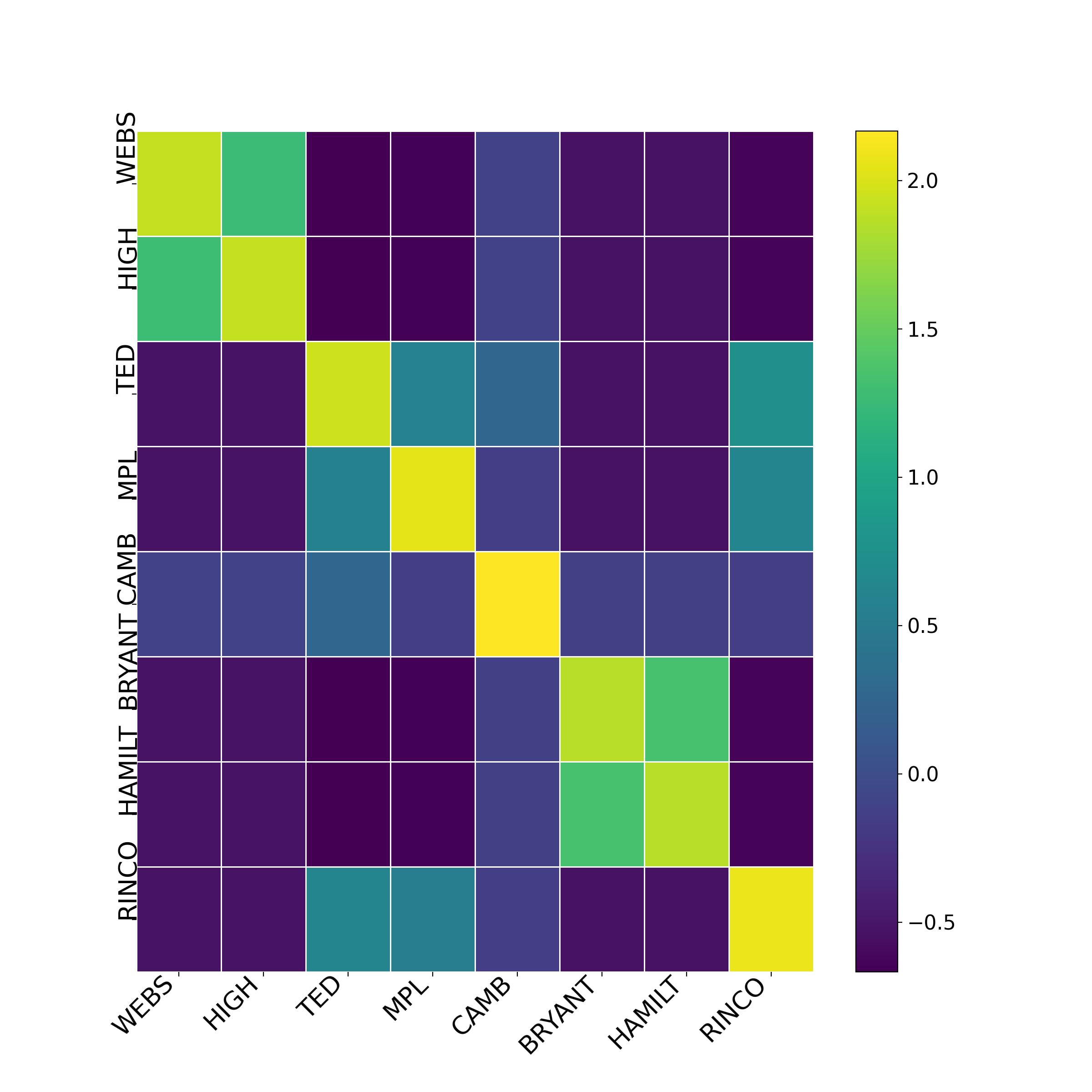
In this paper, is an important parameter that client can use to control the limit of similarity value with other clients. If is extremely small, i.e. , which means that client does not trust any other clients that participate in the FL, and thus it is the same as the local training scenario. On the other hand, If , it means that client totally trusts at least one client that owns the same data distribution as itself. To investigate the influence of , weight within 100 communication rounds are shown in Fig. 4. In this case, ’HIGH’ station is selected as client , and ’RINCO’ is set to be a malicious client that carries out a flipping attack. When is small, e.g. , there are only two clients that contribute to ’HIGH’. As the increases, more clients are assumed to be beneficial to station ’HIGH’, and when , all clients except the malicious one are considered as beneficial, with a different but close weight . It can be concluded that the credit-based method is quite effective, as it can always shut out the malicious clients while attributing different weights depending on their contribution/similarity to the selected client and a self-tuned parameter . In addition, we have visualized the global attention of the 8 stations as a heatmap, which can be seen in Fig.3.

IV-F Influence of the CNN
In the framework, we utilized 1D CNN encoders to extract temporal information and features and then upload them to a server. By employing CNNs, we no longer upload raw data but high-dimensional features, thus protecting data privacy. Addition- ally, to demonstrate the effectiveness of CNNs, we conducted a comparison with LSTM encoders as feature extractors for 6- step demand prediction. We employed a 2-layer LSTM as the LSTM encoder (see Table VI). It can be observed that using CNN encoders yielded superior results in both MIL and ICP compared to LSTM encoders, and CNN encoders are simpler than LSTM encoders. Thus, this validates the effectiveness of CNN encoders.
| Encoder | QS | MIL | ICP |
|---|---|---|---|
| CNN-encoder | 1.3285 | 3.9666 | 0.7651 |
| LSTM-encoder | 1.3267 | 4.0352 | 0.7619 |
IV-G Influence of the increasing number of EV charging stations
To consider the increasing number of EV charging stations, We show the forecasting results of the algorithm with varying numbers of nodes (see Fig. VII). As the number of charging stations increases, the QS loss as well as the MIL decreases, which can indicate the effectiveness of federal learning.
| WEBSTER | MPL | |||||
|---|---|---|---|---|---|---|
| QS | MIL | ICP | QS | MIL | ICP | |
| Num=2 | 1.4676 | 4.5097 | 0.7687 | 1.1729 | 3.7555 | 0.7858 |
| Num=8 | 1.3813 | 4.2209 | 0.7634 | 1.1277 | 3.6281 | 0.7965 |
V Conclusions
In this paper, a novel personalized federated graph learning framework is proposed for multi-horizon EV charging demand forecasting, where both the data privacy and security of different stations are guaranteed. To realize probabilistic forecasting while leveraging the correlation between stations, it is first constructed into a graph neural network, where each station trains a probabilistic forecasting model with quantile regression. Further, the GNN structure is integrated into the federated setting with a central server, in which the model of each station is transmitted to protect data privacy. Moreover, a message-passing aggregation method based on the model similarity among stations is provided in the server to get knowledge from the other stations. Meanwhile, a credit-based method is proposed where the similarity can be tuned adaptively with the guiding of the credit that one station has put on the rest of the participants. The convergence of the proposed federated graph learning framework is provided. Experiment on the public EV charging dataset is used to testify to the effectiveness, while the results demonstrate that the proposed method cannot only improve the test performance but also provide a personalized and robust model for each station against malicious attacks. In the future, we will consider the scalability as well as the methods of accelerate the algorithm of PFGL.
References
- [1] S. Acharya, R. Mieth, R. Karri, and Y. Dvorkin, “False data injection attacks on data markets for electric vehicle charging stations,” Advances in Applied Energy, vol. 7, p. 100098, 2022.
- [2] M. B. Arias and S. Bae, “Electric vehicle charging demand forecasting model based on big data technologies,” Applied energy, vol. 183, pp. 327–339, 2016.
- [3] I. Ullah, K. Liu, T. Yamamoto, M. Zahid, and A. Jamal, “Electric vehicle energy consumption prediction using stacked generalization: An ensemble learning approach,” International Journal of Green Energy, vol. 18, no. 9, pp. 896–909, 2021.
- [4] Z. Yi, X. C. Liu, R. Wei, X. Chen, and J. Dai, “Electric vehicle charging demand forecasting using deep learning model,” Journal of Intelligent Transportation Systems, vol. 26, no. 6, pp. 690–703, 2022.
- [5] T.-Y. Ma and S. Faye, “Multistep electric vehicle charging station occupancy prediction using hybrid lstm neural networks,” Energy, vol. 244, p. 123217, 2022.
- [6] J. Bi, F. Luo, S. He, G. Liang, W. Meng, and M. Sun, “False data injection- and propagation-aware game theoretical approach for microgrids,” IEEE Transactions on Smart Grid, vol. 13, no. 5, pp. 3342–3353, 2022.
- [7] M. Cui, J. Wang, and M. Yue, “Machine learning-based anomaly detection for load forecasting under cyberattacks,” IEEE Transactions on Smart Grid, vol. 10, no. 5, pp. 5724–5734, 2019.
- [8] M. Liu, C. Zhao, J. Xia, R. Deng, P. Cheng, and J. Chen, “Pddl: Proactive distributed detection and localization against stealthy deception attacks in dc microgrids,” IEEE Transactions on Smart Grid, vol. 14, no. 1, pp. 714–731, 2023.
- [9] H. B. McMahan, E. Moore, D. Ramage, S. Hampson, and B. A. y Arcas, “Communication-efficient learning of deep networks from decentralized data,” in AISTATS, 2017.
- [10] M. Alazab, S. P. RM, P. M, P. K. R. Maddikunta, T. R. Gadekallu, and Q.-V. Pham, “Federated learning for cybersecurity: Concepts, challenges, and future directions,” IEEE Transactions on Industrial Informatics, vol. 18, no. 5, pp. 3501–3509, 2022.
- [11] D. Yin, Y. Chen, R. Kannan, and P. Bartlett, “Byzantine-robust distributed learning: Towards optimal statistical rates,” in International Conference on Machine Learning. PMLR, 2018, pp. 5650–5659.
- [12] S. Li, E. C.-H. Ngai, and T. Voigt, “An experimental study of byzantine-robust aggregation schemes in federated learning,” IEEE Transactions on Big Data, pp. 1–13, 2023.
- [13] Z. Wang, H. Xu, J. Liu, Y. Xu, H. Huang, and Y. Zhao, “Accelerating federated learning with cluster construction and hierarchical aggregation,” IEEE Transactions on Mobile Computing, pp. 1–1, 2022.
- [14] Y. He, F. Luo, M. Sun, and G. Ranzi, “Privacy-preserving and hierarchically federated framework for short-term residential load forecasting,” IEEE Transactions on Smart Grid, pp. 1–1, 2023.
- [15] A. Z. Tan, H. Yu, L. Cui, and Q. Yang, “Towards personalized federated learning,” IEEE Transactions on Neural Networks and Learning Systems, pp. 1–17, 2022.
- [16] V. Smith, C.-K. Chiang, M. Sanjabi, and A. S. Talwalkar, “Federated multi-task learning,” in Advances in Neural Information Processing Systems, vol. 30. Curran Associates, Inc., 2017.
- [17] Y. M. Saputra, D. T. Hoang, D. N. Nguyen, E. Dutkiewicz, M. D. Mueck, and S. Srikanteswara, “Energy demand prediction with federated learning for electric vehicle networks,” in 2019 IEEE global communications conference (GLOBECOM). IEEE, 2019, pp. 1–6.
- [18] B. Li, Y. Guo, Q. Du, Z. Zhu, X. Li, and R. Lu, “: Privacy-preserving prediction of real-time energy demands in ev charging networks,” IEEE Transactions on Industrial Informatics, vol. 19, no. 3, pp. 3029–3038, 2023.
- [19] W. Wang, F. H. Memon, Z. Lian, Z. Yin, T. R. Gadekallu, Q.-V. Pham, K. Dev, and C. Su, “Secure-enhanced federated learning for ai-empowered electric vehicle energy prediction,” IEEE Consumer Electronics Magazine, vol. 12, no. 2, pp. 27–34, 2023.
- [20] C. Li, Z. Dong, G. Chen, B. Zhou, J. Zhang, and X. Yu, “Data-driven planning of electric vehicle charging infrastructure: a case study of sydney, australia,” IEEE Transactions on Smart Grid, vol. 12, no. 4, pp. 3289–3304, 2021.
- [21] F. Hüttel, I. Peled, F. Rodrigues, and F. C. Pereira, “Deep spatio-temporal forecasting of electrical vehicle charging demand,” 2021.
- [22] R. Luo, Y. Zhang, Y. Zhou, H. Chen, L. Yang, J. Yang, and R. Su, “Deep learning approach for long-term prediction of electric vehicle (ev) charging station availability,” in 2021 IEEE International Intelligent Transportation Systems Conference (ITSC). IEEE, 2021, pp. 3334–3339.
- [23] Y. Sheng, Q. Guo, M. Liu, J. Lan, H. Zeng, and F. Wang, “User charging behavior analysis and charging facility planning practice based on multi-source data fusion,” Power system automation, vol. 1, p. 24, 2022.
- [24] D. Tang and P. Wang, “Probabilistic modeling of nodal charging demand based on spatial-temporal dynamics of moving electric vehicles,” IEEE Transactions on Smart Grid, vol. 7, no. 2, pp. 627–636, 2015.
- [25] B. Yu, H. Yin, and Z. Zhu, “Spatio-temporal graph convolutional networks: A deep learning framework for traffic forecasting,” in Proceedings of the Twenty-Seventh International Joint Conference on Artificial Intelligence. International Joint Conferences on Artificial Intelligence Organization, jul 2018.
- [26] R. Li, M. Tapaswi, R. Liao, J. Jia, R. Urtasun, and S. Fidler, “Situation recognition with graph neural networks,” in Proceedings of the IEEE international conference on computer vision, 2017, pp. 4173–4182.
- [27] X. Liu, J. Ding, W. Jin, H. Xu, Y. Ma, Z. Liu, and J. Tang, “Graph neural networks with adaptive residual,” Advances in Neural Information Processing Systems, vol. 34, pp. 9720–9733, 2021.
- [28] C. Meng, S. Rambhatla, and Y. Liu, “Cross-node federated graph neural network for spatio-temporal data modeling,” in Proceedings of the 27th ACM SIGKDD conference on knowledge discovery & data mining, 2021, pp. 1202–1211.
- [29] C. T. Dinh, N. Tran, and J. Nguyen, “Personalized federated learning with moreau envelopes,” in Advances in Neural Information Processing Systems, H. Larochelle, M. Ranzato, R. Hadsell, M. Balcan, and H. Lin, Eds., vol. 33. Curran Associates, Inc., 2020, pp. 21 394–21 405. [Online]. Available: https://proceedings.neurips.cc/paper_files/paper/2020/file/f4f1f13c8289ac1b1ee0ff176b56fc60-Paper.pdf
- [30] S. Guo, Y. Lin, N. Feng, C. Song, and H. Wan, “Attention based spatial-temporal graph convolutional networks for traffic flow forecasting,” in Proceedings of the AAAI conference on artificial intelligence, vol. 33, no. 01, 2019, pp. 922–929.
- [31] T. N. Kipf and M. Welling, “Semi-supervised classification with graph convolutional networks,” arXiv preprint arXiv:1609.02907, 2016.
- [32] CityofPaloAlto, “Electric vehicle charging station usage (july 2011- dec 2020). open data. city of palo alto, 2021.” https://data.cityofpaloalto.org/dataviews/257812/electric-vehicle-charging-station-usage-july-2011-dec-2020/, 2021.
- [33] M. N. Fekri, K. Grolinger, and S. Mir, “Distributed load forecasting using smart meter data: Federated learning with recurrent neural networks,” International Journal of Electrical Power & Energy Systems, vol. 137, p. 107669, 2022.
Appendix A Proof of Theorem 1
Based on the L-smooth assumption,
| (20) |
where , and the last equality is obtained by using . Now we bound ,
| (21) |
where follows by the convexity of norm, is obtained by using and follows by Assumption 1, and 3. Denote , then
| (22) |
where follows by using , ; and follows by the convexity of norm; is obtained by using Assumption 2, 3; follows by unrolling and ; and follows by the fact that , . Therefore, we have,
| (23) |
Consequently, is bounded by substituting (23) to (A), . Denote , and ; Substitute to (A), and let , it yields:
| (24) |
Rearrange (A) and sum it over , we have
where is the optimal value of . Therefore, if , then we have :
Moreover, if satisfies , and , then we have .