Exterior stability of Minkowski spacetime with borderline decay
Abstract
In 1993, the global stability of Minkowski spacetime has been proven in the celebrated work of Christodoulou and Klainerman [5]. In 2003, Klainerman and Nicolò [13] revisited Minkowski stability in the exterior of an outgoing null cone. In [22], the author extended the results of [5] to minimal decay assumptions. In this paper, we prove that the exterior stability of Minkowski holds with decay which is borderline compared to the minimal decay considered in [22].
Keywords
Minkowski stability, double null foliation, borderline decay, –weighted estimates.
1 Introduction
1.1 Einstein vacuum equations and the Cauchy problem
A Lorentzian –manifold is called a vacuum spacetime if it solves the Einstein vacuum equations:
| (1.1) |
where denotes the Ricci tensor of the Lorentzian metric . The Einstein vacuum
equations are invariant under diffeomorphisms, and therefore one considers equivalence
classes of solutions. Expressed in general coordinates, (1.1) is a non-linear geometric coupled system of partial differential equations of order 2 for . In suitable coordinates, for example so-called wave coordinates, it can be shown that (1.1) is hyperbolic and hence admits an initial value formulation.
The corresponding initial data for the Einstein vacuum equations is given by specifying a
triplet where is a Riemannian –manifold and is the traceless symmetric –tensor on satisfying the constraint equations:
| (1.2) | ||||
where denotes the scalar curvature of , denotes the Levi-Civita connection of and
In the future development of such initial data , is a spacelike hypersurface with induced metric and second fundamental form .
The seminal well-posedness results for the Cauchy problem obtained in [3, 4] ensure that for any smooth Cauchy data, there exists a unique smooth maximal globally hyperbolic development solution of Einstein equations (1.1) such that and , are respectively the first and second fundamental forms of in .
The prime example of a vacuum spacetime is Minkowski spacetime:
for which Cauchy data are given by
In the present work, we consider the problem of the stability of Minkowski spacetime and start with reviewing the literature on this problem.
1.2 Previous works of the stability of Minkowski spacetime
In 1993, Christodoulou and Klainerman [5] proved the global stability of Minkowski for the Einstein-vacuum equations, a milestone in the domain of mathematical general relativity. In 2003, Klainerman and Nicolò [13] proved the Minkowski stability in the exterior of an outgoing cone using the double null foliation. Moreover, Klainerman and Nicolò [14] showed that under stronger asymptotic decay and regularity properties than those used in [5, 13], asymptotically flat initial data sets lead to solutions of the Einstein vacuum equations which have strong peeling properties. Given that the goal of this paper is to extend the result of [13], we will state the results of [5, 13] in Section 1.3.
We now mention other proofs of Minkowski stability. In 2007, Bieri [2] gave a new proof of global stability of Minkowski requiring one less derivative and less vectorfields compared to [5]. Lindblad and Rodnianski [18, 19] gave a new proof of the stability of the Minkowski spacetime using wave-coordinates and showing that the Einstein equations verify the so called weak null structure in that gauge. Huneau [11] proved the nonlinear stability of Minkowski spacetime with a translation Killing field using generalised wave-coordinates. Using the framework of Melrose’s b-analysis, Hintz and Vasy [9] reproved the stability of Minkowski space. Graf [7] proved the global nonlinear stability of Minkowski space in the context of the spacelike-characteristic Cauchy problem for Einstein vacuum equations, which together with [13] allows to reobtain [5]. Under the framework of [13] and using –weighted estimates of Dafermos and Rodnianski [6], the author [21] reproved the Minkowski stability in exterior regions. More recently, Hintz [8] reproved the Minkowski stability in exterior regions by using the framework of [9]. Using –weighted estimates, the author [22] extends the results of [2] to minimal decay assumption.
There are also stability results concerning Einstein’s equations coupled with non trivial matter fields, see for example the introduction of [21, 22].
1.3 Minkowski Stability in [5, 13]
We recall in this section the results in [5, 13]. First, we recall the definition of a maximal hypersurface, which plays an important role in the statements of the main theorems in [5, 13].
Definition 1.1.
An initial data is posed on a maximal hypersurface if it satisfies
| (1.3) |
In this case, we say that is a maximal initial data set, and the constraint equations (1.2) reduce to
| (1.4) |
We introduce the notion of –asymptotically flat initial data.
Definition 1.2.
Given and , we say that a data set is –asymptotically flat if there exists a coordinate system defined outside a sufficiently large compact set such that:
-
•
In the case of 222The notation means , .
(1.5) -
•
In the case of
(1.6)
We also introduce the following functional:
where is the geodesic distance from a fixed point , and is the Bach tensor, is the traceless part of . Now, we can state the main theorems of [5] and [13].
Theorem 1.3 (Global stability of Minkowski space [5]).
There exists an sufficiently small such that if , then the initial data set , –asymptotically flat (in the sense of Definition 1.2) and maximal, has a unique, globally hyperbolic, smooth, geodesically complete solution. This development is globally asymptotically flat, i.e. the Riemann curvature tensor tends to zero along any causal or spacelike geodesic. Moreover, there exists a global maximal time function and a optical function 333An optical function is a scalar function satisfying . defined everywhere in an external region.
Theorem 1.4 (Exterior stability of Minkowski [13]).
Consider an initial data set , –asymptotically flat and maximal, and assume is bounded. Then, given a sufficiently large compact set such that is diffeomorphic to , and under additional smallness assumptions, there exists a unique future development of with the following properties:
-
•
can be foliated by a double null foliation and whose outgoing leaves are complete.
-
•
We have detailed control of all the quantities associated with the double null foliations of the spacetime, see Theorem 3.7.1 in [13].
1.4 Rough version of the main theorem
In this section, we state a simple version of our main theorem. For the explicit statement, see Theorem 3.3.
Theorem 1.6 (Main Theorem (first version)).
Let an initial data set which is –asymptotically flat in the sense of Definition 1.2. Let a sufficiently large compact set such that is diffeomorphic to . Assume that we have a smallness condition on . Then, there exists a unique future development in its future domain of dependence with the following properties:
-
•
can be foliated by a double null foliation whose outgoing leaves are complete for all .
-
•
We have detailed control of all the quantities associated with the double null foliations of the spacetime, see Theorem 3.3.
1.5 Structure of the paper
-
•
In Section 2, we recall the fundamental notions and the basic equations.
-
•
In Section 3, we present the main theorem. We then state intermediate results, and prove the main theorem. The rest of the paper focuses on the proof of these intermediary results.
-
•
In Section 4, we make bootstrap assumptions and prove first consequences. These consequences will be used frequently in the rest of the paper.
-
•
In Section 5, we apply –weighted estimates to Bianchi equations to control the flux of curvature.
-
•
In Section 6, we estimate the –norms of curvature components and Ricci coefficients using the null structure equations and Bianchi equations.
1.6 Acknowledgements
The author would like to thank Sergiu Klainerman and Jérémie Szeftel for their support, discussions and encouragements.
2 Preliminaries
2.1 Geometry set-up
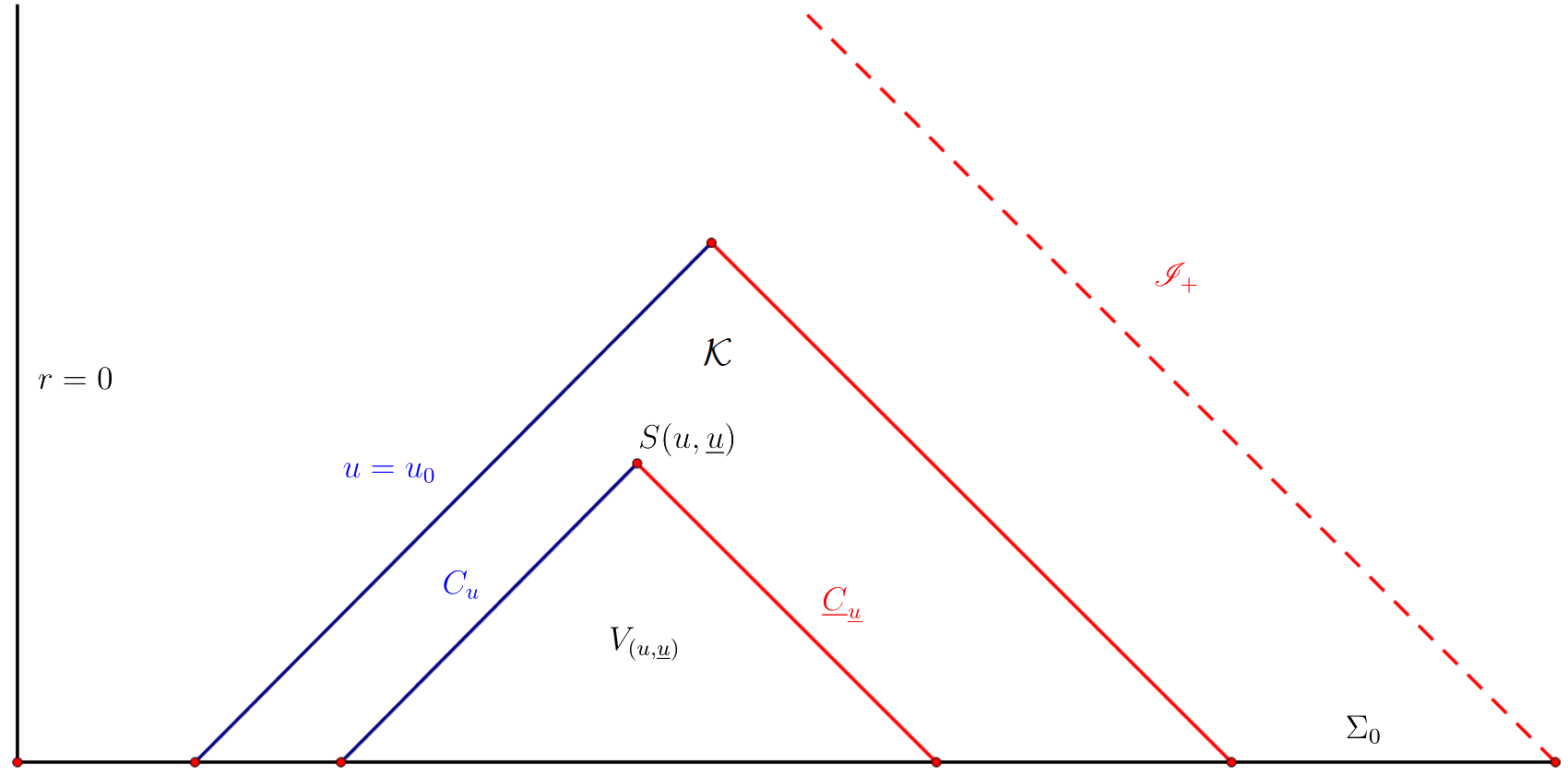
Let be a spacelike hypersurface. Let be a compact subset such that is diffeomorphic to where is the unit closed ball in . We fix a radial foliation on the initial hypersurface by the level sets of a scalar function . The leaves are denoted by
| (2.1) |
where . We assume that
| (2.2) |
where is the area radius of defined by
| (2.3) |
We now construct a double null foliation in the future of . For this, we denote the normal vectorfield of oriented towards the future and the unit vectorfield tangent to , oriented towards infinity and orthogonal to the leaves . We define two null vectors on by
| (2.4) |
We extend the definition of and to the future of by the geodesic equations:
| (2.5) |
We define a positive function by the formula
| (2.6) |
where is called the null lapse function. We then define two optical functions and in the future of by the Eikonal equations
and the initial conditions
We then define the normalized null pair by
| (2.7) |
The spacetime in the future of is then foliated by the level sets of and respectively. We use to denote the outgoing null hypersurfaces which are the level sets of and use to denote the incoming null hypersurfaces which are the level sets of . We also denote
which are spacelike –spheres. On a given two sphere , we choose a local frame , we call a null frame. As a convention, throughout the paper, we use capital Latin letters to denote an index from 1 to 2 and Greek letters to denote an index from 1 to 4, e.g. denotes either or .
For any sphere of the double null foliation , we denote its causal past by
Denoting and taking , we define the bootstrap region by:
By local existence theorem, the spacetime exists if is sufficiently close to . We now introduce a local coordinate system in with . In this coordinates system, the spacetime metric takes the following form:
| (2.8) |
where denotes the induced metric on and denotes the null shift. Note that
We recall the null decomposition of the Ricci coefficients and curvature components of the null frame as follows:
| (2.9) | ||||
and
| (2.10) | ||||
where denotes the Hodge dual of . The null second fundamental forms are further decomposed in their traces and , and traceless parts and :
We define the horizontal covariant operator as follows:
We also define and to be the horizontal projections:
A tensor field defined on is called tangent to if it is a priori defined on the spacetime and all the possible contractions of with either or are zero. We use and to denote the projection to of usual derivatives and . As a direct consequence of (2.9), we have the following Ricci formulae:
| (2.11) | ||||
The following identities hold for the null frame (2.7):
| (2.12) | ||||
see for example (6) in [16].
2.2 Integral formulae
Definition 2.1.
Given a scalar function on , we denote its average and its average free part by
Lemma 2.2.
For any scalar function , the following identities hold:
Taking , we obtain
where is the area radius defined by
2.3 Hodge systems
Definition 2.3.
For tensor fields defined on a –sphere , we denote by the set of pairs of scalar functions, the set of –forms and the set of symmetric traceless –tensors.
Definition 2.4.
Given and , we define their Hodge dual
Definition 2.5.
Given and , we denote
Definition 2.6.
For a given , we define the following differential operators:
Definition 2.7.
We define the following Hodge type operators, as introduced in section 2.2 in [5]:
-
•
takes into and is given by:
-
•
takes into and is given by:
-
•
takes into and is given by:
-
•
takes into and is given by:
We have the following identities:
| (2.13) | ||||
where denotes the Gauss curvature on . See for example (2.2.2) in [5] for a proof of (2.13).
Definition 2.8.
Let , and , we define the weighted angular derivatives :
We also denote for any tensor , ,
Definition 2.9.
For a tensor field on a –sphere , we denote its –norm:
We also introduce the following scale invariant –norm:
2.4 Null structure equations
Definition 2.10.
We define the following renormalized quantity:
| (2.14) | ||||
where is defined by the solution of
We also define the following renormalized curvature components:
| (2.15) |
The mass aspect functions are defined as follows:
| (2.16) |
We also define the following modified mass aspect functions:
| (2.17) |
Proposition 2.11.
We have the following null structure equations:
| (2.18) | ||||
the Codazzi equations:
| (2.19) | ||||
the torsion equation:
| (2.20) |
and the Gauss equation:
| (2.21) |
Proof.
See (3.1)–(3.5) in [16]. ∎
2.5 Bianchi equations
Proposition 2.12.
We have the following Bianchi equations:
Proof.
See (2.7) and (2.8) in [1]. ∎
3 Main theorem
In the sequel of this paper, we always denote
| (3.1) |
3.1 Fundamental norms
We proceed to define our main norms on a given bootstrap spacetime .
3.1.1 Schematic notation , and
Definition 3.1.
We divide the Ricci coefficients into three parts:
We then denote
and for
3.1.2 norms (flux of curvature)
In the remainder of this paper, we always denote and two fixed constants satisfying
For a tensor field defined on or , we denote its –flux by
| (3.2) | ||||
We define the norms of flux of curvature components in the bootstrap region . We denote
where for
It remains to define for
3.1.3 norms (–norms of geometric quantities)
We first define the –norms of , and in the bootstrap region . We define
with
We then define the –norms for the renormalized quantities introduced in Definition 2.10:
with
We also introduce the following auxiliary norm:
Moreover, we define
Finally, we denote
3.1.4 norm (Initial data)
We introduce the following norm on initial hypersurface :
where
3.2 Statement of the main theorem
The goal of this paper is to prove the following theorem.
Theorem 3.3 (Main Theorem).
Consider an initial data set which is –asymptotically flat in the sense of Definition 1.2. Assume that we have on :
| (3.3) |
where is a constant small enough. Then, has a unique development in its future domain of dependence with the following properties:
-
1.
can be foliated by a double null foliation . Moreover, the outgoing cones are complete for all .
-
2.
The norms and defined in Section 3.1 satisfy
(3.4)
3.3 Main intermediate results
Theorem 3.4.
Assume that
| (3.5) |
Then, we have
| (3.6) |
Theorem 3.4 is proved in Section 5. The proof is based on the –weighted method introduced by Dafermos and Rodnianski in [6].
Theorem 3.5.
Assume that
| (3.7) |
Then, we have
| (3.8) |
3.4 Proof of the main theorem
Definition 3.6.
Let the set of spacetimes associated with a double null foliation in which we have the following bounds:
| (3.9) |
Definition 3.7.
We denote the set of values such that .
The assumption and the local existence theorem imply that (3.9) holds if is sufficiently close to . So, we have .
Define to be the supremum of the set . We want to prove . We assume by contradiction that is finite. In particular we may assume . We consider the region . Recall that we have
according to the assumption of Theorem 3.3. Applying Theorem 3.4, we obtain
Then, we apply Theorem 3.5 to obtain
Applying local existence results,666See Theorem 10.2.1 in [5] and Theorem 1 in [20]. we can extend to for a sufficiently small. We denote and the norms in the extended region . We have
as a consequence of continuity. We deduce that satisfies all the properties in Definition 3.6, and so , which is a contradiction. Thus, we have , which implies property 1 of Theorem 3.3. Moreover, we have
in the whole exterior region, which implies property 2 of Theorem 3.3. This concludes the proof of Theorem 3.3.
Remark 3.8.
We have from (3.4)
which implies for small enough that . Hence, we deduce that there is no trapped surface in the exterior region .
4 Bootstrap assumptions and first consequences
In the rest of the paper, we always make the following bootstrap assumptions:
| (4.1) |
4.1 First consequences of bootstrap assumptions
In this section, we derive first consequences of (4.1) in the region . In the sequel, the results of this section will be used frequently without explicitly mentioning them.
Remark 4.1.
According to , we have in the bootstrap region
| (4.2) |
Combining with and , this yields
| (4.3) |
Lemma 4.2.
Under the assumption (4.1), we have the following bounds:
Lemma 4.3.
For two quantities and , we denote
if decays better than for . Then, the following hold:
-
1.
We have
-
2.
We also have
Remark 4.4.
In the sequel, we choose the following conventions:
-
•
Let , for a quantity satisfying the same or even better decay and regularity as , for , we write
-
•
For a sum of schematic notations, we write
if . For example, we write
4.2 Commutation identities
Proposition 4.5.
For any scalar function , we have:
Proposition 4.6.
We have the following schematic commutator identities
4.3 Main equations in schematic form
Proposition 4.7.
We have the following schematic null structure equations:
| (4.4) | ||||
We also have the following transport equations for the quantities defined in Definition 2.10:
| (4.5) | ||||
Proof.
Proposition 4.8.
We have the following schematic Bianchi equations:
4.4 Sobolev inequalities and –estimates
Proposition 4.9.
Let be a tensor field on . Then, we have777Recall that the –flux on and has been defined in (3.2).
Proposition 4.10.
Let be a tensor field on . Then, we have
Proof.
See Lemma 4.1.3 in [13]. ∎
Proposition 4.11.
The following hold for all :
-
1.
Let be a solution of . Then we have
-
2.
Let be a solution of . Then we have
-
3.
Let be a solution of . Then we have
Proof.
See Corollary 2.3.1.1 in [5]. ∎
5 Hyperbolic estimates (proof of Theorem 3.4)
In this section, we prove Theorem 3.4 by the –weighted estimate method introduced in [6] and applied to Bianchi equations in [10, 21, 22].
5.1 Schematic notation , and
We introduce the following schematic notations as in [22].
Definition 5.1.
For a quantity , we denote
if satisfies the following estimates:
Similarly, we denote
if satisfies the following estimates:
Moreover, we denote
if satisfies the following estimate:
For , we also denote , for , if satisfies the same or even better decay and regularity properties as .
Lemma 5.2.
Proof.
The following theorem provides a unified treatment of all the nonlinear error terms in curvature estimates.
Theorem 5.3.
Let , and . We define
| (5.4) |
Then, we have the following properties:
-
1.
In the case , we have
(5.5) -
2.
In the case , we have
(5.6)
5.2 Estimates for general Bianchi pairs
The following lemma provides the general structure of Bianchi pairs.
Lemma 5.4.
Let and , real numbers. Then, we have the following properties.
-
1.
If and satisfying
(5.7) Then, the pair satisfies for any real number
(5.8) -
2.
If and satisfying
(5.9) Then, the pair satisfies for any real number
(5.10)
Proof.
See Lemma 4.2 in [21]. ∎
Remark 5.5.
The following lemma allows us to obtain –decay of curvature flux along .
Lemma 5.6.
For any , we have the following estimate for :
Proof.
Proposition 5.7.
Proof.
We have from Stokes’ theorem
Thus, integrating (LABEL:div) or (LABEL:div2) in , we obtain
Applying Lemma 5.6, we deduce
Recalling from Lemma 5.2 that , we obtain from (5.5) in Theorem 5.3
Recalling from Lemma 4.2 that , we deduce
Combining the above estimates, we infer
Recalling that , we deduce that, for small enough, (LABEL:caseone) and (LABEL:casethree) hold in correspond cases. This concludes the proof of Proposition 5.7. ∎
5.3 Estimates for the Bianchi pair
Proposition 5.8.
We have the following estimate:
| (5.13) |
Proof.
We recall from Proposition 4.8 that
| (5.14) | ||||
Differentiating (5.14) by for and applying Proposition 4.6, we deduce101010The linear term comes from the fact that , see (2.13). We also use the convention .
where is defined by
Note that we have from Lemma 5.2
Hence, we obtain by ignoring the terms which decay better
Applying (LABEL:caseone) with , , , , and noticing that
| (5.15) |
we obtain from Lemma 5.2
| (5.16) | ||||
The linear term on the R.H.S of (LABEL:abestim0) can be easily absorbed by Cauchy-Schwarz and induction. Moreover, applying Theorem 5.3 in the case , , and , and noticing that
we obtain from (5.5)
Injecting it into (LABEL:abestim0), we obtain (5.13). This concludes the proof of Proposition 5.8. ∎
5.4 Estimates for the Bianchi pair
Proposition 5.9.
We have the following estimate:
| (5.17) | ||||
Proof.
We recall from Proposition 4.8
Differentiating it by and applying Proposition 4.6, we deduce
Applying Lemma 5.2, we obtain
Applying (LABEL:casethree) with , , , and , and noticing that
| (5.18) |
we infer from Lemma 5.2
Applying (5.5) in Theorem 5.3, we easily deduce
Combining with (5.13), we obtain
The estimates for and can be deduced similarly. This concludes the proof of Proposition 5.9. ∎
5.5 Estimates for the Bianchi pair
Proposition 5.10.
We have the following estimate:
| (5.19) |
Proof.
We recall from Proposition 4.8
Differentiating it by and applying Proposition 4.6, we deduce
Noticing that we have from Lemma 5.2 and (2.19)
Thus, we have
Applying (LABEL:casethree) with , , , and , we obtain
where we used (5.17), the fact that and Proposition 4.11 in the last step. Thus, we deduce for small enough
Applying (5.5) in Theorem 5.3, we easily deduce
Combining the above estimates, this concludes the proof of Proposition 5.10. ∎
5.6 Estimates for the Bianchi pair
Proposition 5.11.
We have the following estimate:
| (5.20) |
Proof.
We have from Proposition 4.8
Differentiating it by and applying Proposition 4.6, we infer
Note that we have from Lemma 5.2
We also have from Lemma 5.2
Hence, we deduce
Applying (LABEL:casethree) with , , , and , we obtain
where we used (5.19) at the last step. Applying (5.6) in Theorem 5.3, we easily deduce
Moreover, we have from and Proposition 4.11
Combining the above estimates, we obtain for small enough
Combining with Proposition 4.11, this concludes the proof of Proposition 5.11. ∎
6 Transport and –elliptic estimates (proof of Theorem 3.5)
The goal of this section is to prove Theorem 3.5. Throughout this section, we use the following shorthand notations:
6.1 Preliminaries
We recall the evolution lemma, which will be used repeatedly throughout this section.
Lemma 6.1.
Under the assumption , the following holds:
-
1.
Let be –covariant –tangent tensor fields satisfying the outgoing evolution equation
We have for
-
2.
Let be –covariant –tangent tensor fields satisfying the incoming evolution equation
We have for
The following lemma will be useful to estimate the –norms.
Lemma 6.2.
We have for
and for
We also have for
Proof.
6.2 Estimates for curvature
Proposition 6.3.
We have the following estimates:
Proposition 6.4.
We have the following estimates:
Proof.
Proposition 6.5.
We have the following estimates:
Proof.
We have from Proposition 4.8
Differentiating it by and applying Proposition 4.6, we obtain
Note that we have from Proposition 5.10
| (6.1) |
Applying Proposition 4.11 and Lemmas 6.1 and 6.2, we infer
Next, we have from Proposition 4.8
Differentiating it by and applying Proposition 4.6, we deduce
Note that we have from Proposition 5.11
Applying Lemmas 6.1 and 6.2, we infer
This concludes the proof of Proposition 6.5. ∎
6.3 Estimates for , and
Proposition 6.6.
We have the following estimates:
| (6.2) | ||||
Proof.
We have from Proposition 4.7
| (6.3) | ||||
Differentiating (6.3) by and applying Proposition 4.6, we obtain
| (6.4) |
Applying Lemma 6.1, we deduce
Next, differentiating (6.4) by and applying Proposition 4.6, we infer
Note that we have from Proposition 5.8 and Lemma 5.2
| (6.5) |
Applying Lemmas 6.1 and 6.2, we have
This concludes the proof of Proposition 6.6. ∎
Proposition 6.7.
We have the following estimates:
| (6.6) | ||||
Proof.
Proposition 6.8.
We have the following estimates:
| (6.8) | ||||
Proof.
We recall from (2.12) that
| (6.9) |
Applying Lemma 6.1 and Propositions 6.7 and 4.10, we infer
Next, differentiating (6.9) by and applying Proposition 4.5, we obtain
Applying Lemma 6.1 and Proposition 6.7, we deduce
Then, differentiating (6.9) by and applying Proposition 4.6, we have
| (6.10) |
Applying Lemma 6.1 and Proposition 6.7, we obtain
Finally, differentiating (6.10) by and applying Propositions 4.5 and 4.7, we have
Notice that we have from Proposition 5.9
Applying Lemma 6.1 and Proposition 6.6, we deduce
This concludes the proof of Proposition 6.8. ∎
6.4 Estimates for and
Proposition 6.9.
We have the following estimates:
| (6.11) | ||||
Proof.
We recall the following equation from Proposition 4.7:
| (6.12) |
Differentiating (6.12) by and applying Proposition 4.5, we obtain
| (6.13) | ||||
Applying Lemma 6.1 and Proposition 6.6, we obtain
Next, differentiating (6.13) by and applying Proposition 4.6, we infer
| (6.14) |
Applying Lemma 6.1 and Proposition 6.6, we easily obtain
Finally, differentiating (6.14) and applying Proposition 4.5 and Proposition 4.11, we deduce
Notice that we have from Proposition 5.9
Applying Lemmas 6.1 and 6.2, we infer
This concludes the proof of Proposition 6.9. ∎
Proposition 6.10.
We have the following estimates:
| (6.15) | ||||
Proof.
We have from Proposition 4.7:
| (6.16) |
Differentiating (6.16) by and applying Proposition 4.6, we obtain
| (6.17) | ||||
Applying Lemmas 6.1 and Proposition 6.8, we infer
Next, differentiating (6.17) by and applying Proposition 4.5, we deduce
Applying Lemmas 6.1 and 6.2, (6.5) and Proposition 6.8, we deduce
This concludes the proof of Proposition 6.10. ∎
6.5 Estimates for and
Proposition 6.11.
We have the following estimates:
Proof.
We recall from Proposition 4.7
| (6.18) | ||||
Applying Lemma 6.1 and Propositions 6.4, 6.9 and 4.10, we infer
Next, differentiating (6.18) by and applying Proposition 4.5, we deduce
| (6.19) |
Applying Lemma 6.1 and Propositions 6.4 and 6.9, we obtain
Finally, differentiating (6.19) by and applying Proposition 4.6, we obtain
Applying Lemmas 6.1 and 6.2, (6.1) and Propositions 5.10 and 6.9, we obtain
Recalling from (2.16) that
we easily deduce from Propositions 6.9 and 6.10 that
This concludes the proof of Proposition 6.11. ∎
Proposition 6.12.
We have the following estimates:
Proof.
We recall from Proposition 4.7
| (6.20) | ||||
Differentiating (6.20) by and applying Proposition 4.5, we deduce
| (6.21) |
Applying Lemma 6.1 and Propositions 6.3 and 6.10, we infer
Next, differentiating (6.21) by and applying Proposition 4.6, we have
Applying Lemmas 6.1 and 6.2 and Propositions 5.9 and 6.10, we obtain111111Recall that we have and .
Recalling that
we have from Propositions 6.9 and 6.10 that
This concludes the proof of Proposition 6.12. ∎
6.6 Estimates for , , and
Proposition 6.13.
We have the following estimates:
| (6.22) | ||||
We also have
| (6.23) |
Proof.
We recall from Proposition 4.7
Applying Propositions 4.11, we obtain for
Combining with Propositions 6.3, 6.4, 6.11 and 6.12, we obtain (6.22) as stated.
Next, we have from Proposition 2.11
| (6.24) |
Applying Lemma 6.1, (6.22) and Proposition 6.4, we obtain
which implies (6.23). This concludes the proof of Proposition 6.13. ∎
Proposition 6.14.
We have the following estimates:
6.7 End of the proof of Theorem 3.5
Proposition 6.15.
We have the following estimates:
| (6.25) |
Proof.
Proposition 6.16.
We have the following estimate:
Proof.
Proposition 6.17.
We have the following estimates:
Remark 6.18.
Proposition 6.17 implies that the spheres are only almost round at future null infinity .
Proof.
References
- [1] X. An and J. Luk, Trapped surfaces in vacuum arising dynamically from mild incoming radiation, Adv. Theor. Math. Phys. 21 (1), 1–120, 2017.
- [2] L. Bieri, An extension of the stability theorem of the Minkowski space in general relativity, J. Diff. Geom. Vol. 86 (1), 17–70, 2010.
- [3] Y. Choquet-Bruhat, Théorème d’existence pour certains systèmes d’équations aux dérivèes partielles non linéaires, Acta Math. 88, 141–225, 1952.
- [4] Y. Choquet-Bruhat and R. Geroch Global aspects of the Cauchy problem in general relativity, Comm. Math. Phys. 14, 329–335, 1969.
- [5] D. Christodoulou and S. Klainerman, The Global Nonlinear Stability of Minkowski Space, Princeton Mathematical Series 41, 1993.
- [6] M. Dafermos and I. Rodnianski, A new physical-space approach to decay for the wave equation with applications to black hole spacetimes, XVIth International Congress on Mathematical Physics, World Sci. Publ., Hackensack, NJ, 2010, 421–432.
- [7] O. Graf, Global nonlinear stability of Minkowski space for spacelike-characteristic initial data, arXiv:2010.12434.
- [8] P. Hintz, Exterior stability of Minkowski space in generalized harmonic gauge, Arch. Rational Mech. Anal. 247 (99), 2023.
- [9] P. Hintz and A. Vasy, Stability of Minkowski space and polyhomogeneity of the metric, Ann. PDE 6 (1): Art. 2, 146 pp, 2020.
- [10] G. Holzegel, Ultimately Schwarzschildean spacetimes and the black hole stability problem, arXiv:1010.3216.
- [11] C. Huneau, Stability of Minkowski spacetime with a translation space-like Killing field, Ann. PDE 4 (1): Art. 12, 147 pp, 2018.
- [12] A. D. Ionescu and B. Pausader, The Einstein-Klein-Gordon coupled system: global stability of the Minkowski solution, Annals of Mathematics Studies 406, Princeton University Press, 2022.
- [13] S. Klainerman and F. Nicolo, The Evolution Problem in General Relativity, Progress in Mathematical Physics, Vol. 25, 2003.
- [14] S. Klainerman and F. Nicolo, Peeling properties of asymptotic solutions to the Einstein vacuum equations, Classical Quant. Grav. 20, 3215–3257, 2003.
- [15] S. Klainerman and I. Rodnianski, Causal geometry of Einstein-Vacuum spacetimes with finite curvature flux, Invent. math. 159, 437–529, 2005.
- [16] S. Klainerman and I. Rodnianski, On the formation of trapped surfaces, Acta Math 208, 211–333, 2012.
- [17] P. G. LeFloch and Y. Ma, Nonlinear stability of self-gravitating massive fields, arXiv:1712.10045, Accepted in Ann. PDE.
- [18] H. Lindblad and I. Rodnianski, Global existence for the Einstein vacuum equations in wave coordinates, Comm. Math. Phys. 256 (1), 43–110, 2005.
- [19] H. Lindblad and I. Rodnianski, The global stability of Minkowski spacetime in harmonic gauge, Ann. of Math. (2), 171 (3), 1401–1477, 2010.
- [20] J. Luk, On the Local Existence for the Characteristic Initial Value Problem in General Relativity, Int. Math. Res. Not. no. 20, 4625–4678, 2018.
- [21] D. Shen, Stability of Minkowski spacetime in exterior regions, Pure Appl. Math. Q. 20 (2), 757–868, 2024.
- [22] D. Shen, Global stability of Minkowski spacetime with minimal decay, arXiv:2310.07483.