Euclid preparation

LensMC is a weak lensing shear measurement method developed for Euclid and Stage-IV surveys. It is based on forward modelling to deal with convolution by a point spread function with comparable size to many galaxies; sampling the posterior distribution of galaxy parameters via Markov Chain Monte Carlo; and marginalisation over nuisance parameters for each of the 1.5 billion galaxies observed by Euclid. The scientific performance is quantified through high-fidelity images based on the Euclid Flagship simulations and emulation of the Euclid VIS images; realistic clustering with a mean surface number density of $\qty{250}{arcmin^{-2}}$ ($I_{\scriptscriptstyle\rm E}<29.5$) for galaxies, and $\qty{6}{arcmin^{-2}}$ ($I_{\scriptscriptstyle\rm E}<26$) for stars; and a diffraction-limited chromatic point spread function with a full width at half maximum of $0.\mathrm{″}2$ and spatial variation across the field of view. Objects are measured with a density of $\qty{90}{arcmin^{-2}}$ ($I_{\scriptscriptstyle\rm E}<26.5$) in $4500\,\unit{deg^{2}}$. The total shear bias is broken down into measurement (our main focus here) and selection effects (which will be addressed elsewhere). We find: measurement multiplicative and additive biases of $m_{1}=(-3.6\pm 0.2)\times 10^{-3}$, $m_{2}=(-4.3\pm 0.2)\times 10^{-3}$, $c_{1}=(-1.78\pm 0.03)\times 10^{-4}$, $c_{2}=(0.09\pm 0.03)\times 10^{-4}$; a large detection bias with a multiplicative component of $1.2\times 10^{-2}$ and an additive component of $-3\times 10^{-4}$; and a measurement PSF leakage of $\alpha_{1}=(-9\pm 3)\times 10^{-4}$ and $\alpha_{2}=(2\pm 3)\times 10^{-4}$. When model bias is suppressed, the obtained measurement biases are close to Euclid requirement and largely dominated by undetected faint galaxies ($-5\times 10^{-3}$). Although significant, model bias will be straightforward to calibrate given the weak sensitivity.

1 Introduction

Weak gravitational lensing by large-scale structure is a mature cosmological tool to measure its distribution of dark matter and study dark energy through the evolution with redshift (Schneider, 2006; Kilbinger, 2015; Mandelbaum, 2018). Weak lensing is particularly sensitive to modifications of the theory of gravity or the emergence of physics beyond the concordance $\Lambda$-cold dark matter model, which affect the clustering of dark matter (Amendola et al., 2018).

Galaxies surveys from the ground, such as the Dark Energy Survey (DES, Abbott et al., 2018b), the Kilo Degree Survey (KiDS, Kuijken et al., 2015), and the Hyper Suprime-Cam survey (HSC, Aihara et al., 2017), are now achieving constraints on the dark matter sector (primarily in the $\Omega_{\text{m}}$–$\sigma_{8}$ parameter space and their combination $S_{8}$) to a few percent (Abbott et al., 2018a; Hildebrandt et al., 2017; Hikage et al., 2019). After extensive consistency checks and sensitivity studies, recent lensing measurements from galaxy surveys have been shown to be broadly in agreement with each other, but in mild tension with the Planck satellite at the $2\,\sigma$ level or greater (Aghanim et al., 2020; Joudaki et al., 2020; Amon et al., 2022; Heymans et al., 2021; Asgari et al., 2021; Loureiro et al., 2022), including the latest joint analysis of DES and KiDS (Abbott et al., 2023).

In the coming years, galaxy surveys will enter a new regime of area, depth, and image quality. The space-based Euclid telescope (survey area of $14\,000\,\unit{\deg^{2}}$, full width at half maximum resolution of $0.\mathrm{″}2$, depth of 24.5, $I_{\scriptscriptstyle\rm E}$+$Y_{\scriptscriptstyle\rm E}J_{\scriptscriptstyle\rm E}H_{\scriptscriptstyle\rm E}$ filters, see Laureijs et al., 2011; Cropper et al., 2016; Euclid Collaboration: Scaramella et al., 2022); the planned space-based Roman telescope ($1700\,\unit{\deg^{2}}$, $0.\mathrm{″}2$, 26.5, YJH+F184, see Spergel et al., 2015); and the ground-based Rubin Observatory Legacy Survey of Space and Time (LSST, $18\,000\,\unit{\deg^{2}}$, $0.\mathrm{″}7$, 27.5, $ugrizy$, see Ivezić et al., 2019) will substantially increase the number of observable galaxies compared to current surveys. The systematic observation of a billion galaxies or more across one third of the visible sky will then be possible for the first time. The combined effect of improved survey area and angular resolution will be an enhanced ability to probe both the large and small scales via weak lensing and galaxy clustering, allowing us to constrain cosmological models and dark energy to percent level precision (Mandelbaum et al., 2018; Euclid Collaboration: Blanchard et al., 2020), or even an order of magnitude better when combined with data from Planck (Euclid Collaboration: Ilić et al., 2022).

With such a dramatic improvement in precision that will be achieved in the coming years, experiments are now focussing on understanding the accuracy of their analyses (see, e.g., Euclid Collaboration: Paykari et al., 2020). Along with theory uncertainties, the cosmic shear measurement and redshift estimation are the most challenging aspects of any large-scale weak lensing surveys. The concern of this paper is on cosmic shear measurement, which provides the necessary data for the weak lensing cosmological analysis (Kilbinger, 2015). In order to achieve of order one percent precision on the dark energy equation of state, a billion galaxies or more with median redshift around $1$ need to be observed. This observation has to be carried out consistently so the same shape measurement procedure is applied to all objects. This measurement has to be conducted with outstanding accuracy to satisfy the stringent requirement of $2\times 10^{-3}$ and $3\times 10^{-4}$ on the measured multiplicative and additive shear biases that were set in the early development phase of weak lensing space telescopes (Massey et al., 2012; Cropper et al., 2013).

Throughout the years, a number of shear measurement methods have been developed, tested on data challenges, and applied to real data. These can be categorized in two main classes: non-parametric and parametric. Among the non-parametric is Kaiser-Squires-Broadhurst (KSB, Kaiser et al., 1995) based on weighted moments of image data. Because of its simplicity, these estimators were used for the very first attempts at measuring cosmic shear in the early 2000s. These methods are fast, so can be quickly calibrated, but sensitive to effects which need to be characterised. Later on, with better precision, it became clear that more effects needed to be factored in, particularly a realistic point spread function (PSF) and the sensitivity of bias on PSF ellipticity, known as leakage. Parametric methods, based on forward modelling and model fitting, soon appeared to be better suited to accurately incorporate such real data features building on solid statistical grounds. In recent years, a more systematic use of model fitting techniques has been observed across all major lensing surveys. The Bayesian-inspired shape method lensfit (Miller et al., 2007; Kitching et al., 2008; Miller et al., 2013) has been extremely successful, first in the Canada-France Hawaii Telescope Lensing Survey (CFHTLenS, Heymans et al., 2012), and then more recently also KiDS. This is based on forward modelling and marginalisation over galaxy nuisance parameters. A similar method is IM3SHAPE (Zuntz et al., 2013), a maximum likelihood estimator based again on analytic forward models that has been applied to DES. While lots of real-data effects, including the PSF, are accounted for and can directly be built in parametric methods, any in-built correction clearly introduces extra computational overhead as the parameter probability distribution needs to be sampled accurately.

While lensing measurements have become more precise over time, accuracy has also needed to be examined more carefully. Methods have been compared in data challenges and have run on common simulations with increasing realism, such as in the Shear TEsting Programme (STEP, Heymans et al., 2006; Massey et al., 2007) and the Gravitational LEnsing Accuracy Testing (GREAT, Bridle et al., 2010; Kitching et al., 2012; Mandelbaum et al., 2015). With no method outshining in absolute terms, and methods being better at some aspects of the measurement but worse at others, it has become evident that some form of calibration is still necessary. The field has become reliant on galaxy simulations more than ever. Sophisticated high-fidelity simulations now need to reproduce the realism of actual observations as close as possible, so all biases from detection, measurement, and selection can be fully captured (Fenech Conti et al., 2017; Kannawadi et al., 2019; Euclid Collaboration: Martinet et al., 2019; MacCrann et al., 2021; Li et al., 2023a, b). Calibration naturally raises the question about how sensitive our results are to the assumptions we make in our simulations (Hoekstra et al., 2017), or how large these simulations need to be to meet the desired precision (Pujol et al., 2019; Jansen et al., 2024). Other methods now rely on some form of calibration that is directly built in the measurement process. Galaxy images used in calibration are either simulated internally, inferred from real data, or a combination of the two. Metacalibration (Sheldon & Huff, 2017; Huff & Mandelbaum, 2017) derives internal estimates of the sensitivity of the ellipticity estimator to input shears and has been extremely successful on DES Year 3 (Gatti et al., 2021); Bayesian Fourier Domain (BFD, Bernstein & Armstrong, 2014; Bernstein et al., 2016) estimates the Taylor coefficients of the galaxy likelihood expanded over shear with information about moments measured from calibration fields; a similar implementation to BFD uses forward modelling (Sheldon, 2014); the KiDS self-calibration (Fenech Conti et al., 2017) derives internal estimates of the ellipticity bias from noise-free galaxy images; MomentsML relies on simulated images to train shear-predicting artificial neural networks (Tewes et al., 2019). Because many selection biases happen before the shear measurement introduces its own bias, the field has gradually become more aware that those will probably be the limiting factor in future lensing surveys. Further work around Metacalibration has led to Metadetection to address the issue (Sheldon et al., 2020). An application of the method to Euclid-like simulations has shown that while selection biases may exceed requirements, the outlook is still positive with demonstrated success at handling detection and blending biases (Hoekstra, 2021; Hoekstra et al., 2021; Melchior et al., 2021).

The impact of neighbours to lensing measurements has also become one of the most important issues that current and future surveys will need to address. In space, the large number density of detected galaxies of about $\qty{30}{arcmin^{-2}}$ ($I_{\scriptscriptstyle\rm E}<24.5$) is compensated by a good image resolution, so the impact of neighbours may not be as bad as on ground. In fact, due to the worse resolution on the ground, the impact of neighbours is serious, affecting $60\%$ of the sample (Bosch et al., 2017; Arcelin et al., 2020). DES Year 1 results (Samuroff et al., 2017) showed that the total neighbour bias can be as large as $9\%$ (reaching $80\%$ at a close distance to the neighbour, if uncorrected). Cuts to the catalogue to remove those objects can reduce the total bias to $1\%$ (reaching $30\%$ at a close distance to the neighbour), however at the cost of reducing the effective number density by $30\%$ and leaving a residual bias on $S_{8}$ of $2\,\sigma$. While Metacalibration has been extremely successful in a few idealised cases (e.g.  isolated galaxies) and Metadetection in the handling of blending and detection bias, a suite of advanced simulations have been required for the tomographic calibration of DES Year 3 (MacCrann et al., 2021). These have shown that an external calibration is still required, as the unresolved neighbour introduces correlation between the two galaxies at different redshift, plus the Metacalibration shear responses will be biased by the presence of the neighbour itself. Therefore calibration simulations have been made necessary to correctly capture neighbour bias and the interplay between shear and redshift. However, these simulations assume uniform random distributions of galaxies that have been reweighted to mimic clustering, which raises the question that the inferred bias may likely be underestimated. The most recent simulations by KiDS have realistic clustering of $N$-body simulations, mimic a number of measurement effects, and address the shear-redshift interplay (Li et al., 2023a). With a larger number density it is expected that the situation may be more serious in future surveys.

In this paper we present our advanced shear measurement method LensMC, specifically developed for Euclid, that builds upon the knowledge and success of ground-based measurement at handling real data effects. Similarly to lensfit, it adopts a mean estimator. Contrarily to lensfit, it does not marginalise over nuisance parameters with numerical approximations. With full flexibility in the choice of the prior, all the marginalisation in LensMC is performed by Markov Chain Monte Carlo (MCMC) sampling, for individual galaxies or jointly across groups of neighbouring galaxies. While IM3SHAPE returns the maximum of the likelihood estimated via the Levenberg-Marquardt algorithm, LensMC employs a combination of large-scale and small-scale algorithms, conjugate gradient and simplex methods, to estimate a suitable initial guess for the MCMC sampling, thus requiring no information about the model derivatives and dramatically reducing the sensitivity on the initial guess (which is assumed always the same for all galaxies). The galaxy models in LensMC are rendered directly in the Fourier space, hence only a single Fourier transform is required. A recent profile-fitting method, The Farmer, has also drawn attention recently (Weaver et al., 2023). This method is a maximum likelihood estimator, whose position and shape initial guesses are provided by the detection method. It includes a decision tree based on $\chi^{2}$ values to classify objects on their likely type and provides error estimates via Cramer-Rao bounds. Preliminary results are encouraging, however the method has not been tested to full space-based cosmic shear accuracy yet.

Accurate cosmic shear measurement requires controlling the bias from a number of sources. Key examples are: source clustering, faint objects, neighbours, PSF leakage, image artefacts, and cosmic rays. Additionally, any forward-modelling methods is plagued by potential model bias. One of the main sources of model bias is addressed here. In summary, LensMC employs: (i) forward modelling to deal with Euclid image undersampling and convolution by a PSF with comparable size to many galaxies; (ii) joint measurement of object groups to correctly handle bias due to neighbours; (iii) masking out objects belonging to different groups; (iv) MCMC sampling to sample the posterior in a multi-dimensional parameter space, calculate weights, and correctly marginalise ellipticity over nuisance parameters and other objects in the same group. We particularly focus on the realism of our simulations, including clustering, stars, object detection, the handling of neighbours due to the high number density, and the use of realistic undersampled chromatic PSF images with spatial variation across the field of view. We do not include further real data effects such as non-linearities or cosmic rays as these will be addressed separately. Also we assume the same broadband PSF as obtained from a spectral energy distribution (SED) of an SBc-type galaxy at redshift of 1 in both simulations and measurements.

Sect. 2 introduces our method and the practical advantages in addressing real data problems. Our forward-modelling method is sufficiently fast to analyse the typical data volume of Stage-IV surveys and can be applied to the complexity of Euclid measurements, including undersampled data and a complex PSF, while accounting for the full degrees of freedom in the galaxy modelling. Additionally, it allows the proper handling of resolved neighbours by joint measurement and masking of more distant galaxies, stars, and artefacts in the images. Sect. 3 describes the simulations used for our intensive testing of the method. The images are fiducial realisations of the Euclid VIS detector and galaxies are rendered based on $N$-body simulations with full variability of the morphological properties. All galaxies are convolved with a realistic pre-flight PSF model with full spatial variation, but ignoring the chromatic variability. Sect. 4 presents the main results of this testing. When model bias, chromaticity, and selection biases are suppressed, the obtained biases are close to Euclid requirement. This measurement bias is largely dominated by undetected faint galaxies in the images. The bias is also found to be stable and mostly insensitive to the many effects in the simulations. As the Euclid analysis will also need to correct for other artefacts in the images, the residual bias will be straightforward to calibrate through image simulations. Once we include the model bias by allowing the full variability in the galaxy models, the overall bias becomes significant. However, since the sensitivity is weak (the derivative of the bias with respect to the assumptions made in the simulations appears negligible), it will then be straightforward to also calibrate the model bias through image simulations. Sect. 5 discusses the main findings and draws the conclusions of our work.

2 Method

The main physical quantity of interest in weak lensing is the reduced cosmic shear (Kilbinger, 2015),

$$g=\frac{\gamma}{1-\kappa}\leavevmode\nobreak\ ,$$ (1)

where $\kappa$ and $\gamma$ are convergence and shear (both related to the gravitational potential), and $g\approx\gamma$ in the weak lensing regime. The related observable in weak lensing is the ellipticity of a galaxy,

$$\epsilon=\frac{a-b}{a+b}\mathrm{e}^{2\mathrm{i}\varphi}\leavevmode\nobreak\ ,$$ (2)

where $a$ and $b$ are, respectively, the semi-major and semi-minor axes, $\varphi\in\left[0,\pi\right)$ is the orientation angle of the galaxy, and $|\epsilon|\leq 1$. The effect of weak lensing is to distort the ellipticity of a source galaxy, $\epsilon_{\text{s}}$, by the canonical transformation (Seitz & Schneider, 1997),

$$\epsilon=\frac{\epsilon_{\text{s}}+g}{1+\epsilon_{\text{s}}\,g^{*}}\leavevmode\nobreak\ ,$$ (3)

where all spin-2 quantities are expressed in complex notation, e.g., $\epsilon=\epsilon_{1}+\mathrm{i}\,\epsilon_{2}$, where $\epsilon_{1}$ quantifies the distortion along $x$ and $y$, and $\epsilon_{2}$ along the coordinate axes rotated by $\pi/4$. As it is customary in weak lensing, we will refer to $\epsilon_{\text{s}}$ as the intrinsic ellipticity of the source galaxy, and $\epsilon$ as the lensed or observed ellipticity. The ellipticity in Eq. (3) is a point estimate for shear in that information on the underlying cosmic shear can be derived in a statistical sense as a sample average, $g=\langle\epsilon\rangle$, which holds whenever the distribution of orientation angles is uniform, e.g., when there are no astrophysical intrinsic alignments (Joachimi et al., 2015) or shear dependent selection effects.

In weak lensing measurements we infer the reduced shear through sample averages. In this work, we use the ellipticity as a point estimator for shear and the problem of measuring ellipticity can be formulated fully in Bayesian terms. Suppose we have a pixel data vector, $\boldsymbol{D}$, and a model for the galaxy brightness distribution, $\boldsymbol{I}=\boldsymbol{I}(\epsilon,\theta,\phi)$, as a function of ellipticity, $\epsilon$, intrinsic nuisance parameters, $\theta$, and linear nuisance parameters, $\phi$. Thanks to Bayes’ theorem, we can define a joint posterior as follows,

$$p(\epsilon,\theta,\phi|\boldsymbol{D})=\frac{p(\boldsymbol{D}|\epsilon,\theta,\phi)p(\epsilon,\theta,\phi)}{p(\boldsymbol{D})}\leavevmode\nobreak\ ,$$ (4)

where $p(\boldsymbol{D}|\epsilon,\theta,\phi)$ is the likelihood, $p(\epsilon,\theta,\phi)$ is the prior on ellipticity and nuisance parameters, and $p(\boldsymbol{D})$ is the evidence or marginal likelihood,

$$p(\boldsymbol{D})=\int p(\boldsymbol{D}|\epsilon,\theta,\phi)p(\epsilon,\theta,\phi)\,\text{d}\epsilon\,\text{d}\theta\,\text{d}\phi\leavevmode\nobreak\ .$$ (5)

We can then construct the ellipticity marginal posterior

$$p(\epsilon|\boldsymbol{D})=\frac{1}{p(\boldsymbol{D})}\int p(\boldsymbol{D}|\epsilon,\theta,\phi)p(\epsilon,\theta,\phi)\,\text{d}\theta\,\text{d}\phi\leavevmode\nobreak\ ,$$ (6)

marginalising out the nuisance parameters. Common choices of estimators are the maximum likelihood or maximum posterior probability, but these are usually biased if the distribution is not Gaussian. However, the bias can be predicted in simple cases of low dimensionality or when the probability function is fully analytic (Cox & Snell, 1968; Hall & Taylor, 2017). Another option that has been successful in ground-based surveys (Miller et al., 2013) is to set our estimator to the mean of the posterior distribution,

$$\hat{\epsilon}=\int\epsilon\,p(\epsilon|\boldsymbol{D})\,\text{d}\epsilon\leavevmode\nobreak\ .$$ (7)

We will adopt this definition as it has some useful properties:

1. as the nuisance parameters are marginalised out, their impact on the ellipticity estimator via their correlation is mitigated;

2. overfitting is inherently reduced as we pick an average representative of all possible realisations that are statistically equivalent;

3. following on from the previous point, we expect the mean estimator to be, in general, less biased than the maximum estimators;

4. the mean of the distribution can be estimated through MCMC sampling techniques (see Sect. 2.3); such estimators satisfy the central limit theorem and therefore converge to the true mean.

We will discuss more about those points later in this section. Whatever choice is made, any estimator can be seen as a non-linear mapping between $\boldsymbol{D}$ and $\epsilon$. Therefore even if $\boldsymbol{D}$ were to be Gaussian distributed, the estimator will not, hence leading to a fundamental bias in the measurement, which has been commonly referred to as noise bias (Melchior & Viola, 2012; Refregier et al., 2012; Viola et al., 2014). Moreover, as the shear is estimated through an sample average over a population of galaxies with varying morphological properties and complex selections, the properties of the shear bias will be different from that of galaxy ellipticity. Assuming shear is small, it is customary in the field to model the shear bias on each component with a linear model (Guzik & Bernstein, 2005; Huterer et al., 2006; Heymans et al., 2006),

$$\hat{g}_{i}=(1+m_{i})\,g_{i}+c_{i}+n_{i}\leavevmode\nobreak\ ,$$ (8)

where $m_{i}$ and $c_{i}$ are the multiplicative and additive biases for the $i$-th component, $g_{i}$ is the true shear, $\hat{g}_{i}$ is an estimate of it, and $n_{i}$ is the corresponding statistical noise. The transformation in Eq. (8) should in principle have $m_{i}$ replaced by a matrix $m_{ij}$ to model any potential cross-talk between shear components. Alternatively, it could be rewritten as a spin-2 equation (Kitching & Deshpande, 2022),

$$\hat{g}=(1+m_{0})\,g+m_{4}\,g^{*}+c+n\leavevmode\nobreak\ .$$ (9)

However, generalising upon previous work, $m_{0}$ and $m_{4}$ are now spin 0 and 4 complex operators, where $m_{0}=|m_{0}|\exp[2\,i\,\sigma_{0}]$, $m_{4}=|m_{4}|\exp[4\,i\,\sigma_{4}]$, and $\sigma_{0}$ and $\sigma_{4}$ are angles. Physically, this added flexibility allows for complete mode-mixing: $m_{0}$ models a dilation and rotation of the true shear, whereas $m_{4}$ models a reflection around the axis determined by its phase. We defer the application of this approach to future work. Multiplicative terms can be induced by, e.g., non-Gaussianities in the posterior (skewness at first order), caused by, e.g., pixel noise and a small galaxy size relative to the PSF. Additive terms are due to anisotropies induced by, e.g., the PSF and its spatial variability across the field of view. This effect is referred to as PSF leakage and is defined by the dependence of $c_{i}$ on the PSF ellipticity $\epsilon_{\text{PSF},i}$ (see, e.g., Gatti et al., 2021, and references therein),

$$\alpha_{i}=\frac{\,\text{d}c_{i}}{\,\text{d}\epsilon_{\text{PSF},i}}\leavevmode\nobreak\ .$$ (10)

We focus primarily on the $c$ dependence on $\epsilon_{\text{PSF}}$ as instead the $m$ dependence is negligible as long as the PSF is stable and its variation in size is within a percent levels. Earlier studies (Massey et al., 2012; Cropper et al., 2013) have set out requirements for space-based missions on $m$ and $c$ based on a top-down error breakdown from cosmology to two-point statistics. For Euclid, the requirement is on the statistical error on bias, $\sigma_{m}<2\times 10^{-3}$ and $\sigma_{c}<3\times 10^{-4}$. That is roughly equivalent to saying that a shear of $1\%$ should be measured with a fractional accuracy and precision of $0.2\%$. Note that the requirement is an order of magnitude more stringent than current ground-based experiments (Hildebrandt et al., 2017). The detailed breakdown of the total budget on $m$ and $c$ into various error terms (Cropper et al., 2013) suggests we can set the required statistical error on the bias due to the measurement alone to $\sigma_{m}<5\times 10^{-4}$ and $\sigma_{c}<5\times 10^{-5}$. Therefore, in order to measure $|g|\approx 0.03$ with a residual post-calibration multiplicative bias smaller than $\sigma_{m}$, one will need at least $n=\sigma_{\epsilon}^{2}\,|g|^{-2}\sigma_{m}^{-2}\approx 4\times 10^{8}$ galaxies, where $\sigma_{\epsilon}\approx 0.3$ is the ‘shape noise’, i.e., the standard deviation of the per-component intrinsic ellipticity distribution. Obviously measurement noise and intrinsic scatter in the morphological properties will also need to be factored in. A ballpark estimate for the Euclid requirement on PSF leakage that we will be using as benchmark in our analysis is $\sigma_{\alpha}\lesssim\sigma_{c}/\left|\delta\epsilon_{\text{PSF}}\right|$, where $|\delta\epsilon_{\text{PSF}}|\approx 0.1$ is the order of magnitude (absolute) variation in PSF ellipticity across the field of view, which yields $\sigma_{\alpha}<1\times 10^{-3}$ if we assume a budget of $\sigma_{c}<1\times 10^{-4}$. This derivation may be too conservative, as a full propagation of the errors and biases through to cosmological parameters has been demonstrated to be able to capture the spatial pattern imprinted by the PSF and other effects (Euclid Collaboration: Paykari et al., 2020). Other surveys have implemented other solutions such a first-order expansion on PSF ellipticity and PSF model residuals in KiDS (Heymans et al., 2006; Giblin et al., 2021) or the angular correlations between PSF ellipticity and size implemented in the rho statistics in DES (Jarvis et al., 2020).

In the next subsections we address the key elements of the LensMC measurement method: galaxy modelling, PSF convolution, likelihood, sampling, and a further discussion about handling real data effects. We emphasise the role of joint measurement of objects to address neighbour bias, which is a concern for current and upcoming surveys, and also our MCMC strategy to sample a multi-dimensional parameter space and marginalise each lensing target over all nuisance parameters and other objects.

2.1 PSF-convolved galaxy models

We assume 2D-projected galaxy models as a mixture of two circular Sérsic profiles (Sérsic, 1963), for disc,

$$I_{\text{d}}(r)\propto\exp\left(-\frac{r}{r_{\text{e}}}\right)\leavevmode\nobreak\ ,$$ (11)

and bulge,

$$I_{\text{b}}(r)\propto\exp\left[-a_{\text{b}}\left(\frac{r}{r_{\text{h}}}\right)^{\frac{1}{n_{\text{b}}}}\right]\leavevmode\nobreak\ ,$$ (12)

where $r$ is the distance from the centre, $r_{\text{e}}$ is the exponential scale length of the disc, $r_{\text{h}}$ is the bulge half-light radius, $n_{\text{b}}=1$, and $a_{\text{b}}\approx 2\,n_{\text{b}}-0.331$ (Peng et al., 2002). The bulge Sérsic index is fixed to $1$ based on recent multi-wavelength observations of the Hubble CANDELS/GOODS-South field (Welikala et al., in prep.), while bulge profiles with $n_{\text{b}}=4$ (de Vaucouleurs) are instead more typical for early-type galaxies at low redshift. Both profiles are normalised so that their integral is 1. In the measurement, $r_{\text{e}}$ plays the role of object size parameter, and we fix the bulge-to-disc scale length ratio to $r_{\text{h}}/r_{\text{e}}=0.15$ based on the same Hubble Space Telescope measurements (Welikala et al., in prep.). Finally, we impose a hard cut-off on the surface brightness profile at $r_{\max}/r_{\text{e}}=4.5$ since observations indicate that galaxies have truncated surface brightness distributions (Van der Kruit & Searle, 1981, 1982). The parameters $n_{\text{b}}$, $r_{\max}/r_{\text{e}}$, and $r_{\text{h}}/r_{\text{e}}$ are assumptions made in the modelling that can potentially lead to large biases in presence of a mismatch in the assumed Sérsic index compared to simulations (Simon & Schneider, 2017). We stress that our choice of fixed values are based on recent observations, and the model bias due to incorrect assumptions are often intertwined with the particular simulation setup and its complexity. A detailed investigation of sensitivity of the calibration to bulge parameters is presented later in this paper.

The Sérsic model introduced above is an isotropic profile with zero ellipticity. To make it anisotropic, i.e., elliptical with ellipticity $\epsilon=\epsilon_{1}+\mathrm{i}\,\epsilon_{2}$, we use the following distortion matrix

$$\mathsf{S}=\frac{\bar{r}_{0}}{q_{\epsilon}\,r_{0}}\begin{pmatrix}1-\epsilon_{1}&-\epsilon_{2}\\ -\epsilon_{2}&1+\epsilon_{1}\end{pmatrix}\leavevmode\nobreak\ ,$$ (13)

where $r_{0}/\bar{r}_{0}$ is the scale factor necessary to scale a model of size $\bar{r}_{0}$ to the desired size $r_{0}$. Because observed galaxy shapes are a 2D visual projection of an intrinsically 3D distribution, we introduce the additional scale factor, $q_{\epsilon}=1-|\epsilon|$, to make the profile semi-major axis invariant under ellipticity transformation. Discs and bulges typically show different intrinsic ellipticity. As discs will be observed more elliptical if edge-on, their ellipticity is primarily driven by inclination angle. In contrast, bulges are spheroids that are almost invariant under inclination, so they will appear more circular. In the measurement, we still apply the same ellipticity to both components as part of our 2D modelling, but we are aware that a positive ellipticity gradient from the intrinsically 3D distribution would induce a bias if not fully captured (Bernstein, 2010). Our ellipticity estimate will therefore be a proxy of the inclination angle, especially for disc-dominated galaxies. Any residual ellipticity gradient, if significant, will have to be addressed separately as part of the calibration.

The Euclid telescope, optical elements, and detector introduce distortions of the input galaxy brightness distribution, which must be corrected. The effect is mostly convolutive, which tends to blur the galaxy image further. An example of a typical PSF image for a space-based telescope like Euclid is given in Fig. 1. This is: (i) close to being diffraction limited; (ii) undersampled due to the half width being comparable with the pixel size; (iii) chromatic due to the integration over a wide range of wavelengths in the VIS filter; (iv) SED dependent due to integration being weighted by a combination of galaxy bulge and disc SEDs; (v) spatially variant across the field of view due to optical distortions at the exit pupil; and (vi) epoch variant due to varying Solar aspect angle throughout the mission inducing thermal distortion on the optics. A comprehensive study of the modelling will be presented elsewhere (Duncan et al., in prep.). A smaller contribution also comes from the CCD pixel response function, which models the response of the detector pixel as an integrated measure of the incoming flux illuminating individual pixels. In forward modelling, we include all the convolutive effects due to the telescope PSF and CCD, individually for bulge, disc, and for each image exposure. Colour gradients originate from incorrectly using the total galaxy SED when generating the PSF image, while the bulge and disc will have naturally different SEDs (Semboloni et al., 2013; Er et al., 2018). Using individually PSF-convolved model components may help to control colour gradients, if individual SEDs were available. However, the impact of colour dependence and gradients on our analysis is not addressed here since we assume the same broadband PSF as obtained from an SED of an SBc-type galaxy at redshift 1 in both simulations and measurements. Further non-linear distortions, such as in the case of charge transfer inefficiency (CTI, Rhodes et al., 2010) and the brighter-fatter effect (BFE, Antilogus et al., 2014), are typically corrected for at the image pre-processing stage, but residuals could still affect the shear measurement (Massey et al., 2014; Israel et al., 2015), which we do not include here.

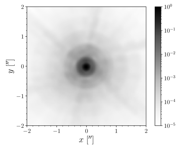
Figure 1: Example of a Euclid chromatic PSF for an assumed SED of a SBc-type galaxy at redshift 1. The flux in the image is rescaled to its maximum value, and oversampled by a factor 3 with respect to the native VIS pixel size of $0.\mathrm{″}1$. Diffraction spikes are clearly visible at a significant distance from the centre, despite the blurring due to the chromaticity. The full width at half maximum (FWHM), including its variation across the field of view, is $$$^{+0.0040}_{-0.0019}$, comparable with the Euclid pixel size, so images will be undersampled at the Nyquist limit. The ellipticity is $\epsilon_{1,\text{PSF}}=0.017^{+0.038}_{-0.024}$ and $\epsilon_{2,\text{PSF}}=0.001^{+0.042}_{-0.020}$, with the superscript and subscript denoting absolute ranges.

Galaxy modelling for large-volume surveys like Euclid requires fast and efficient rendering of the images. All operations described so far are best suited to work in the Fourier space. We adopt a similar approach to galsim (Rowe et al., 2015). Consider the generic profile $I(r)$, which could be either Eq. (11) or (12). Because of its isotropy, the 2D Fourier transform is the 1D Hankel transform,

$$\tilde{I}(k)=2\pi\int_{0}^{\infty}I(r)\,\text{J}_{0}(kr)\,r\,\text{d}r\leavevmode\nobreak\ ,$$ (14)

where $k$ is the Fourier frequency (sampled on an oversampled grid) and $\text{J}_{0}$ is the Bessel function of the first kind. We call $\tilde{I}(k)$ the template model which any profile with arbitrary choice of parameter values (ellipticity, size, and position offset) can be derived from. To render a galaxy profile with parameters $\epsilon_{1}$, $\epsilon_{2}$, and $r_{\text{e}}$, we apply the inverse distortion matrix $\mathsf{S}^{-1}$ to coordinates in Fourier space, so anisotropic coordinates are now defined by $\boldsymbol{k}^{\prime}=\mathsf{S}^{-1}\boldsymbol{k}$. A position shift by $\boldsymbol{\delta r}=(\delta x,\delta y)$ from the centre is equivalent to the phase $\boldsymbol{k}^{\prime}\cdot\boldsymbol{\delta r}$. The sheared-stretched-shifted model becomes

$$\tilde{I}^{\prime}(\boldsymbol{k^{\prime}})=\frac{1}{\det\mathsf{S}}\,\mathrm{e}^{-2\pi\mathrm{i}\,\boldsymbol{k}^{\prime}\cdot\,\boldsymbol{\delta r}}\,\tilde{I}(k^{\prime})\leavevmode\nobreak\ ,$$ (15)

where $\tilde{I}(k^{\prime})$ is the template calculated at the sheared-stretched Fourier mode $\boldsymbol{k^{\prime}}$. Since isotropy is lost through the operation above, $\tilde{I}^{\prime}(\boldsymbol{k^{\prime}})$ is no longer a Hankel transform but a full Fourier transform, which is a function of the vector $\boldsymbol{k^{\prime}}$. Note that if $\tilde{I}(k)$ is precomputed and stored in a cached array, then this step will also involve interpolating at the new coordinates. The interpolation error in the convolved model can be seen at a large radius from the centre, but is around the same level of the precision used to store the model itself. We alleviate the problem of undersampling by calculating the PSF and galaxy model on coordinates with a common oversampling factor of 3. It is worth noting that, contrarily to the analytic approach adopted by galsim, our template models are numerical arrays obtained by a Fourier transform of the isotropic model arrays. The main reason for this approach is that the theoretical definition of Hankel transform of Eq. (14) is invalidated by the finite limit of integration and the oversampling of the model, which make our models a bit more realistic. Finally, the oversampled models for PSF and galaxy are multiplied together, the convolved model is downsampled by the same factor to the actual pixel scale, and the downsampled convolved model is inverse fast Fourier transformed to real space.

We further optimise the calculation of the models for speed by drawing on square images of size proportional to the galaxy size being rendered, so larger galaxies require larger arrays. Given a cut-off at $r_{\max}=4.5\,r_{\text{e}}$ from the centre, a minimum image half-size of $2\,r_{\max}$ is required to avoid aliasing from the Fourier transform. Therefore the minimum image size will always be larger than $18\,r_{\text{e}}$. As galaxies are expected to have mean size of $0.\mathrm{″}3$, but spanning the whole range from just below resolution, $0.\mathrm{″}1$, to the largest (although rare) galaxies, $1\mathrm{″}$, we define a template bank of pre-calculated Hankel transforms of circular objects of different scale lengths $\bar{r}_{0}=\{0.2,0.4,0.8,1.6,3.2\}\,\unit{\arcsec}$ and model arrays of different sizes $\{3.2,4.8,6.4,9.6,12.8,19.2,25.6,38.4\}\,\unit{\arcsec}$. To avoid aliasing from the interpolation, the template scale length $\bar{r}_{0}$ is required to be slightly larger than the galaxy size being rendered; we require $\bar{r}_{0}>\sqrt{2}\,r_{\text{e}}$. We apply the operations of shear and stretch to this template bank to get any object of arbitrary ellipticity and size before the convolution with the PSF takes place as previously discussed.

The final galaxy model is a linear mixture of PSF-convolved co-centred components. Let us label the profiles with a subscript ‘d’ for disc and ‘b’ bulge,

$$I(r)=F_{\text{d}}\,I_{\text{d}}(r)+F_{\text{b}}\,I_{\text{b}}(r)\leavevmode\nobreak\ ,$$ (16)

where $F_{\text{d}}$ and $F_{\text{b}}$ are disc and bulge fluxes, and $F=F_{\text{d}}+F_{\text{b}}$ is the total flux. If B/T is the bulge fraction, then the fluxes are also defined by $F_{\text{d}}=F(1-\text{B/T})$ and $F_{\text{b}}=F\;\text{B/T}$.

To summarise, given pre-computed template models for disc and bulge, we can generate a galaxy model with a desired ellipticity, size, and position by carrying out all the operations with simple algebra in Fourier space on oversampled coordinates, and then take one Fourier transform each time at the end. This is sufficiently fast for an intensive, repeated calculation of the same model with varying realisations of galaxy parameters (ellipticity, size, position offset, and fluxes). However, we keep $n_{\text{b}}$, $r_{\max}/r_{\text{e}}$, and $r_{\text{h}}/r_{\text{e}}$ fixed in our modelling as allowing too much freedom would induce strong degeneracies between parameters and complicate the measurement substantially. We address the model bias sensitivity in Sect. 4.4.

2.2 Likelihood

Suppose we have multi-exposure image data vectors $\boldsymbol{D}=\{\boldsymbol{D}_{\text{exp}}\}$. We wish to estimate the model, $\boldsymbol{I}=\{\boldsymbol{I}_{\text{exp}}\}$, that best represents the available exposures. The model $\boldsymbol{I}=\boldsymbol{I}(\epsilon,\theta,\phi)$ is a function of ellipticity $\epsilon=(\epsilon_{1},\epsilon_{2})$, nuisance parameters $\theta=(r_{\text{e}},\delta x,\delta y)$, and linear flux nuisance parameters $\phi=(F_{\text{d}},F_{\text{b}})$.

Assuming Gaussian data, the likelihood can be written as

$$\ln p(\boldsymbol{D}|\epsilon,\theta,\phi)\propto-\frac{1}{2}\Big{[}\boldsymbol{D}-\boldsymbol{I}(\epsilon,\theta,\phi)\Big{]}^{\top}\mathsf{C}^{-1}\Big{[}\boldsymbol{D}-\boldsymbol{I}(\epsilon,\theta,\phi)\Big{]}\leavevmode\nobreak\ ,$$ (17)

where $\mathsf{C}$ is the noise covariance matrix usually estimated from the data as a block diagonal matrix, and the normalisation constant, $1/2\ln[(2\pi)^{\lambda}\det\mathsf{C}]$ ($\lambda$ is the dimensionality), has been ignored. The noise is intrinsically non-stationary since various noise sources (such as the Poisson noise from the objects in the image) vary spatially. Because the model is linear in the component fluxes, $\boldsymbol{I}=F_{\text{d}}\,\boldsymbol{I_{\text{d}}}+F_{\text{b}}\,\boldsymbol{I_{\text{b}}}$, it is straightforward to integrate over the fluxes, $\phi=(F_{\text{d}},F_{\text{b}})$, and we have the following marginalised likelihood,

$$\ln p(\boldsymbol{D}|\epsilon,\theta)\propto\frac{1}{2}\,\mathcal{F}^{-1}_{ij}(\epsilon,\theta)\,\rho_{i}(\epsilon,\theta)\,\rho_{j}(\epsilon,\theta)\leavevmode\nobreak\ ,$$ (18)

where $i$ indexes the model component, $\rho_{i}(\epsilon,\theta)=\boldsymbol{D}^{\top}\mathsf{C}^{-1}\boldsymbol{I}_{i}(\epsilon,\theta)$ is a $2\times 1$ vector, $\boldsymbol{I}_{i}=\partial\boldsymbol{I}/\partial F_{i}$ ($i=\text{d},\text{b})$, and $\mathcal{F}_{ij}$ is the $2\times 2$ Fisher matrix,

$$\mathcal{F}_{ij}(\epsilon,\theta)=\boldsymbol{I}_{i}(\epsilon,\theta)^{\top}\mathsf{C}^{-1}\boldsymbol{I}_{j}(\epsilon,\theta)\leavevmode\nobreak\ .$$ (19)

Note that because the right-hand side of Eq. (18) is quadratic in $\rho_{i}$ and $\mathcal{F}_{ij}$ is positive definite, we find $\ln p(\boldsymbol{D}|\epsilon,\theta)>0$. A full derivation of the marginalised likelihood, including edge cases and implementation, can be found in Appendix A. The dimensionality of the problem has now been reduced from 7 free parameters to 5: ellipticity, size, and position offsets.

Forward modelling provides solid grounds for a further generalisation to measuring multiple objects jointly, especially if they are observed within a short angular separation such as for neighbours. We label each likelihood with the index $\omega$ running through the objects being jointly measured, $\ln p_{\omega}(\boldsymbol{D}|\epsilon,\theta,\phi)$. The joint likelihood is then

$$\ln p(\boldsymbol{D}|\{\epsilon,\theta,\phi\}_{\omega})=\sum_{\omega}\ln p_{\omega}(\boldsymbol{D}|\epsilon,\theta,\phi)\leavevmode\nobreak\ ,$$ (20)

where $\{\epsilon,\theta,\phi\}_{\omega}$ is the set of all parameters for all the objects being measured. In the above equation we assume the independence of the individual likelihoods. This is a fair assumption since close neighbours will very often be so due to random visual alignment. Consequently, those galaxies will be at different redshift and have different shear. A much smaller fraction will include tidal interaction. In this case, the galaxies will be at the same redshift and have the same shear. It it then expected to have some degree of correlation between the individual likelihoods. In more extreme but much rarer cases, the galaxies will be tidally interacting and therefore our Sèrsic modelling would break down entirely as we do not include any extra correlation term. Despite affecting a very small fraction of objects, dedicated simulations would be required to assess the impact on shear bias. Also, it is worth noting that we need to be careful with the marginalisation of the individual likelihoods. The main issue lies in the marginalised likelihood of Eq. (18). This relies on calculating $\rho_{i}(\epsilon,\theta)$ for the various model components. However, when multiple objects are present in the same neighbourhood, this quantity will effectively introduce correlation between the likelihoods of the two objects. Therefore the statistical independence required to multiply likelihoods together will not be ensured. We have verified in testing that not marginalising individual likelihoods is indeed the correct approach to the problem. The joint likelihood is defined in a $7\times N$-dimensional parameter space, where $N$ is the number of objects being measured jointly, with $N=2$ being a typical number found in testing. For increased stability, we first optimise the likelihood for fluxes and positions offsets, and then also for ellipticity and sizes. This proves to be very robust as opposed to iterating over individual objects after masking neighbours to achieve a reliable initial guess (Drlica-Wagner et al., 2018). One key benefit of MCMC is that it marginalises the ellipticity of an object over all remaining nuisance parameters, which include object nuisance parameters as well as the parameters of the other objects included in the joint sampling (see Sect. 2.3).

Our prior is based on enforcing hard bounds on all parameters: $0\leq|\epsilon|<1$ given that the modulus of ellipticity in Eq. (2) cannot exceed 1; $0\leq r_{\text{e}}\leq$$$, where the upper bound is based on observations made in the Hubble Deep Fields; position offsets are restricted to $\pm\,$$$ since the accuracy to which detections are made is typically sub-pixel; and fluxes are positive. A more informative prior could be derived from real observations in the future. A summary of all parameters, being free, fixed or derived, is presented in Table 1.

Table 1: Summary of free, fixed and derived parameters in the modelling. The value should be interpreted as an initial guesses or constant depending on whether the parameter is allowed to vary or remain constant.

	Free	Fixed	Derived	Initial value	Bounds	Unit	Description
$\epsilon_{1}$	✓			0	$|\epsilon|<1$		first component of ellipticity in the tangent plane to $(-\alpha,\delta)$ as defined in Eq. (13)
$\epsilon_{2}$	✓			0	$|\epsilon|<1$		second component of ellipticity in the tangent plane to $(-\alpha,\delta)$ as defined in Eq. (13)
$r_{\text{e}}$	✓			0.3	$[0,2]$	arcsec	effective radius: disc scale length as defined in Eq. (13)
$\Delta\alpha$	✓			0	$[-0.3,0.3]$	arcsec	offset in right ascension as a phase prefactor in Eq. (15)
$\Delta\delta$	✓			0	$[-0.3,0.3]$	arcsec	offset in declination as a phase prefactor in Eq. (15)
$\alpha$			✓			degree	right ascension
$\delta$			✓			degree	declination
$F_{\text{d}}$	✓				$F_{\text{d}}\geq 0$		disc flux: marginalised over or free as defined in Eq. (16)
$F_{\text{b}}$	✓				$F_{\text{b}}\geq 0$		bulge flux: marginalised over or free as defined in Eq. (16)
$F$			✓		$F\geq 0$		total flux
B/T			✓		$[0,1]$		bulge fraction as defined in text after Eq. (16)
S/N			✓		$\text{S/N}\geq 0$		signal-to-noise ratio
$I_{\scriptscriptstyle\rm E}$			✓				magnitude: depends on the assumed zero-point, exposure gain and integration time
$n_{\text{b}}$		✓		1			Sérsic index of the bulge as defined in Eq. (12)
$a_{\text{b}}$		✓		depends on $n_{\text{b}}$			Sérsic coefficient of the bulge as defined in Eq. (12), see Peng et al. (2002)
$r_{\text{h}}/r_{\text{e}}$		✓		0.15			bulge half-light radius to effective radius ratio as defined in text after Eq. (12), see Welikala et al., in prep.
$r_{\text{max}}/r_{\text{e}}$		✓		4.5			truncation radius to effective radius ratio as defined in text after Eq. (12)

2.3 Massive Markov Chain Monte Carlo sampling

Shear measurement poses serious difficulties in identifying the best strategy to sample the posterior probability distribution of Eq. (4), assuming the likelihood of Eq. (18) or (20),

1. since the lensing sample is very broad in morphological properties, it will contain both low and high S/N objects, whose posterior probability distribution can be either very broad or very narrow; hence any sampling strategy must be robust to this variability;

2. the dimensionality of the problem is $7\times N$, where $N$ is the number of objects being measured jointly to mitigate neighbour bias; sampling must then be resilient to the large dimensionality, and provide marginalisation and error estimations with minimum overheads;

3. the shape of the distribution is a strong function of object parameters, such as ellipticity and size, and therefore it varies significantly across the sample; without prior knowledge of the physical properties of each galaxy, any sampling method must run in a consistent, robust way;

4. given the large sample size of order $10^{9}$ galaxies, sampling the posterior is a computational challenge, so a trade-off between method complexity, runtime, and access to computing resources must be identified;

5. the sampling must be completely automated, without human supervision, and no fine tuning of sampling parameters and options is allowed.

Considering all these challenges, our priority must be the average convergence property of the sampler. The best strategy identified is MCMC, which allows us to sample the posterior generated from the marginalised likelihood of Eq. (18) for an individual object, or the joint likelihood of Eq. (20) for a group of objects in an efficient and consistent way, for all $10^{9}$ objects in the sample (hence the adjective ‘massive’). More importantly, MCMC seems to be the best choice to tackle neighbours, particularly as an estimate can be found in a high dimensional parameter space. It is worth noting that another key benefit of MCMC sampling is that it is both a maximisation and sampling procedure. The maximisation happens during the burn-in phase where the sampler tries to reach the region of higher probability. The actual sampling happens in the later stage of the chain after the burn-in phase. The marginalisation over nuisance and error estimation are then natural by-products with no extra overhead. This implies that not only can ellipticity estimates be marginalised over object nuisance parameters, but also over other object parameters in the joint group, hence minimising the impact of neighbours in the final ellipticity estimate.

When searching for such an algorithm that could potentially suit our needs, we have considered a number of potential candidates that are widely used in cosmology and other fields (MacKay, 2002). The development of various sampling methods has primarily been driven by the quest to achieve lower auto-correlation and higher acceptance rate (Hastings, 1970; Swendsen & Wang, 1986; Skilling, 2006; Goodman & Weare, 2010; Foreman-Mackey et al., 2013; Betancourt, 2017; Karamanis & Beutler, 2021; Lemos et al., 2022). Although appealing, all these methods do suffer from increased complexity, which is the limiting factor in large-scale applications, where ‘large’ in this context implies runs repeated over a billion times. Even for the most sophisticated methods, it is often realised that a good initial guess is the key for good sampling of the posterior.

For shear measurement on the scale of large galaxy surveys, there is not much room for sampling complexity. The method has to be light enough and yet robust to all the posteriors that need to be sampled. Furthermore, the likelihood runtime limits the maximum number of samples that can be drawn for each galaxy without having an overall impact on the survey analysis runtime. The likelihood runtime is mostly dominated by the model component generation. The measurement is dominated by sampling the posterior, plus some additional pre-processing, therefore to limit the galaxy runtime to around few seconds per galaxy, the MCMC sampling must be sparse. This is considered acceptable as we are interested in accurate shear estimates, which are found by averaging over ellipticity measurements. We choose an improved version of the Metropolis-Hastings algorithm, which has been modified in two ways: (i) it incorporates some of the ideas of parallel tempering (Swendsen & Wang, 1986; Sambridge, 2013), so the parameter space can be sampled on a larger scale initially, and then on the smaller scale; (ii) it updates the proposal distribution during the burn-in phase, automatically tuning it to find a good match with the target distribution. Let $\vartheta$ be the generic vector of all parameters. As explained in Sect. 2.2, this is $\vartheta=(\epsilon,\theta)$ for individual galaxy measurement or $\vartheta=(\epsilon,\theta,\phi)$ when jointly measuring groups of galaxies. Taking the logarithm of Bayes’ theorem we have

$$\ln p(\vartheta|\boldsymbol{D})\propto\ln p(\boldsymbol{D}|\vartheta)+\ln p(\vartheta)\leavevmode\nobreak\ ,$$ (21)

where the evidence has been ignored since our method is invariant to it. The parameter vector at the current iteration step is denoted with $\vartheta_{t}$, where $t=0,\ldots$ is the MCMC sample index. We also define a tempering function, $T_{t}$, as a function of $t$. This acts as a Boltzmann temperature and its expression will be defined later in the text. When the temperature is high, $T_{t}\gg 1$, sampling from the posterior is equivalent to sampling globally from the prior. When the temperature is gradually reduced, as in annealing, $T_{t}\rightarrow 1$, we begin sampling directly from the posterior. We define such a tempering function for application during the burn-in phase only, and make sure $T_{t}=1$ for the final part of the chain where we will take sample from. The method goes as follows:

1. at $t$, draw a new sample $\vartheta^{\prime}_{t}$ from the proposal distribution $q(\vartheta^{\prime}_{t}|\vartheta_{t})$; here we assume a symmetric Gaussian proposal with mean $\vartheta_{t}$ and a pre-defined diagonal covariance of $10^{-4}$ on all parameters (in units of arcsec for size and position offsets);

2. calculate the logarithm of the acceptance ratio

   $$\ln A=\frac{\ln p(\boldsymbol{D}|\vartheta^{\prime}_{t})-\ln p(\boldsymbol{D}|\vartheta_{t})}{T_{t}}+\ln p(\vartheta^{\prime}_{t})-\ln p(\vartheta_{t})\leavevmode\nobreak\ ;$$ (22)

3. accept or reject $\vartheta^{\prime}_{t}$ with probability $A$, i.e., draw $u$ from the uniform distribution on $[0,1]$ and accept $\vartheta^{\prime}_{t}$ if $u<\min(1,A)$; to speed things up and avoid calculating the likelihood outside the prior, we immediately reject $\vartheta^{\prime}_{n}$ if $p(\vartheta^{\prime}_{n})=0$.

For consistency, all posteriors are sampled from an initial guess that is a circular galaxy of mean size, $r_{\text{e}}=$$$, and zero offset from the nominal position in the sky. If we were to run any MCMC method from this point onward we would end up with varying autocorrelation time depending on how far the actual galaxy is from the initial guess, therefore we would need to wait longer for very elliptical, small, or large galaxies. To improve the convergence of the chains within a smaller number of iterations, we get a better initial guess by running an initial maximisation of the posterior before the actual MCMC. We run the conjugate-gradient search method (Powell, 1964) restricted to only 100 function evaluations, and then a downhill simplex search (Nelder & Mead, 1965). The burn-in phase of the MCMC starts right afterwards. During this phase the temperature is gradually lowered to 1. We adopt the following power law cooling scheme (Cornish & Porter, 2007),

$$T_{t}=\begin{cases}10^{\,f_{\text{heat}}(1-t/t_{\text{cool}})},&\text{if}\leavevmode\nobreak\ t<t_{\text{cool}}\\ 1,&\text{otherwise}\end{cases}\leavevmode\nobreak\ ,$$ (23)

where $f_{\text{heat}}=10$ is the heat factor and $t_{\text{cool}}=100$ is cooling-down sample index. The parameter $t_{\text{cool}}$ represents the number of samples it takes for the tempering function to become 1. Note that $T_{0}=10^{\,f_{\text{heat}}}$ and $T_{t_{\text{cool}}}=1$. We begin with a diagonal Gaussian proposal of width 0.01 on all parameters, which is then recalculated from the chains every 100 samples and rescaled by the factor $2.4\,{\lambda}^{-1/2}$, with $\lambda$ being the number of parameters (Dunkley et al., 2005). The burn-in phase lasts for a total of 500 samples, which is long enough for the tempering function to become 1, the proposal covariance to be recalculated 5 times, and the chain to stabilise and reach the high probability region (well before we start accumulating the final chain samples). The final phase lasts for an additional $N_{\scriptscriptstyle\rm MC}=200$ samples. Again, this is plenty to estimate both the mean and covariance of the chains with enough precision, but we recognise that sampling noise may still be non-negligible.

A good quantitative way to test the convergence of the chains is to investigate their auto-correlation. We do so for a variety of galaxies and results are shown in Appendix B. A less quantitative way is to verify that the acceptance rate is within the expected range. We have also increased the final 200 samples up by a factor 5, without noticing any significant difference in the shear results. For further verification, we have compared the method with our implementation of affine invariant (Goodman & Weare, 2010) and parallel tempering (Swendsen & Wang, 1986; Sambridge, 2013). While these methods produce better ellipticity chains, they have not shown any significant advantage in recovering shear, but increased complexity and therefore runtime overhead.

Once the samples are drawn from the distribution function, calculating the mean and width of the marginalised distribution becomes straightforward. Our point estimate for ellipticity component marginalised over nuisance is the mean of the chain after the burn-in phase,

$$\hat{\epsilon}_{i}=\frac{1}{N_{\scriptscriptstyle\rm MC}}\sum_{t}\epsilon_{i,t}\leavevmode\nobreak\ ,$$ (24)

where $i=1,2$, and $\epsilon_{1,t}$ and $\epsilon_{2,t}$ are the two ellipticity chains. The marginalised ellipticity covariance matrix is

$$C_{ij}=\frac{1}{N_{\scriptscriptstyle\rm MC}-1}\sum_{t}(\epsilon_{i,t}-\hat{\epsilon}_{i})\,(\epsilon_{j,t}-\hat{\epsilon}_{j})\leavevmode\nobreak\ .$$ (25)

We calculate the averaged per-component variance (ignoring negligible covariance between components),

$$C_{\epsilon}=\frac{1}{2}(C_{11}+C_{22})\leavevmode\nobreak\ ,$$ (26)

and choose to define the galaxy shear weight by

$$w=\frac{1}{C_{\epsilon}+\sigma_{\epsilon}^{2}}\leavevmode\nobreak\ ,$$ (27)

where $\sigma_{\epsilon}$ is the assumed shape noise, i.e., the width of the 1D intrinsic ellipticity distribution, ideally estimated in tomographic bins from deeper measurements. We note the negligible sensitivity to the choice of the $1/2$ factor in $C_{\epsilon}$. The MCMC provides a convenient and efficient way to calculate both the mean and width of the ellipticity posterior at no extra computational cost. The weights can then be used to define sample averages, such as in 1-point estimates:

$$\hat{g}_{i}=\frac{1}{\sum_{k}w_{k}}\sum_{k}w_{k}\,\hat{e}_{i,k}\leavevmode\nobreak\ ,$$ (28)

where $k$ indexes the galaxies in the lensing catalogue. The generalisation to 2-point estimates is straightforward. Please note that any choice of weight leads to shear bias due to correlation with the measured ellipticity, and this is tested later in the paper.

We have also implemented the self-calibration of ellipticity proposed by Fenech Conti et al. (2017) via importance sampling and likelihood ratio while checking the quality of the sampling weights (Wraith et al., 2009), without finding strong evidence of improvement. As results will be dominated by other larger effects, we leave out further discussion from this paper.

2.4 Handling real data

Handling real data requires being careful with additional aspects of the measurement. For instance, throughout our discussion we have proposed that our sampling strategy is best suited to handle the presence of neighbours, i.e., resolved objects close to the lensing targets. However, the situation is complicated by the fact that there is more variety in real data as the brightness distribution of an object can be contaminated in different ways depending on the nature of the nearby objects:

1. neighbours (resolved galaxies or stars);

2. blends (unresolved galaxies or stars);

3. any other contamination (cosmic rays, transients, or ghosts).

Each case leads to a particular type of bias, and therefore we deal with close objects in two ways. First, neighbours are grouped with a friend-of-friend algorithm to a maximum angular separation of $r_{\text{friend}}=$$$. If the separation is too small, the objects will be mostly measured in isolation, therefore they will still be affected by the neighbours due to improper masking. If the separation is too large, the groups will begin to be unmanageable in size, but the benefit in controlling the neighbour bias will be negligible. We find that $1\mathrm{″}$ is a good trade-off between measuring $N$ close neighbours jointly within a default postage stamp size of $38.\mathrm{″}4$, and the non-negligible overhead in sampling a $7\times N$ dimensional posterior. The joint analysis of object groups also gives us a good control of neighbour bias, leading to a correction of $m\approx-7\times 10^{-4}$ as it will be shown later in the paper. Second, the segmentation maps and masks that are usually provided with the data (Bertin et al., 2020; Kümmel et al., 2020) are combined in a binary map and passed on to the likelihood to mask out objects in different groups. Detector artefacts or cosmic rays are also masked out in a similar way. In this case, to be even more conservative, we further dilate the masks by one pixel so most of contamination bias should be taken care of. But masking also helps partially with blends because objects that are false negatives by the detection strategy may sometimes be true positives by the masking procedure and therefore be masked out. Blending with faint galaxies has been demonstrated to be relevant when trying to calibrate methods that are particularly sensitive to the problem (Euclid Collaboration: Martinet et al., 2019). We demonstrate that, to some extent, this is also the case in our simulations where we measure objects deeper than the Euclid nominal survey depth, as we will show in the next section.

Real images have a background level that needs to be subtracted. LensMC uses the background estimates and noise maps that the Euclid processing provides, but residual local background variations are subtracted at the individual object group level. This is implemented by post-masking median subtraction. Likewise, the standard deviation of the background noise is estimated after masking. We measure galaxies and stars with the same model described earlier in this section. We find that good star-galaxy separation is based on selecting objects whose measured size is greater than the PSF size. This method fits well with joint measurement of groups, however at the price of rejecting faint galaxies that would anyway have negligible weight or be hard to distinguish from faint stars. More details will be given in Sect. 4.

A measurement is made in sky coordinates using the supplied world coordinate system (WCS) solution, which includes both linear and non-linear distortions (Greisen & Calabretta, 2002). We assume the default coordinate system $(-\alpha,\delta)$, where $\alpha$ is the right ascension and $\delta$ is the declination. We measure position offsets from the provided nominal position in arcsec. The resulting $\alpha$ and $\delta$ are reported in degrees, and $r_{\text{e}}$ in arcsec. Likewise, the measured ellipticity is defined in the tangent plane to the $(-\alpha,\delta)$ coordinate system centred at the object position. We use the WCS to estimate a local linear approximation of the mapping from sky coordinates to tangent plane coordinates at the nominal position. We define 9 points in a square grid of size $0.\mathrm{″}3$ in pixel coordinates centred at the nominal position, map them to sky coordinates, and finally map the sky coordinates back to the undistorted tangent plane. The Jacobian matrix, which models the local linear approximation of the mapping, is the least square solution to the mapping from sky coordinates to tangent coordinates. As part of this procedure, we also calculate the astrometric offsets due to the exposures being dithered differently. The brightness model is then correctly generated taking into account both the local distortion and astrometric offsets so all the observables are measured uniquely in tangent plane to sky coordinates.

When reporting our measurement we always compute $\chi^{2}=-2\ln p/\nu$, where $p$ is the likelihood of Eq. (18) or (20) calculated at the mean estimate and $\nu$ is the number of degrees of freedom. The $\chi^{2}$ will not in general follow the theoretical distribution for a number of reasons. The noise is only approximately Gaussian and non-Gaussianities will always be present in the data. For instance, key examples are the Poisson noise from the background and the object, digitalisation noise, non-linear artefacts, modelling mismatches, or failures in the sampling. Nonetheless, the $\chi^{2}$ metric defined in this way is still a good statistical measure of the quality of the measurement. We also compare the $\chi^{2}$ calculated above with the same quantity, which we call $\chi^{2}_{\text{bkg}}$, after having masked out all the objects, which is expected to be just noise. Objects will be flagged up if the $\chi^{2}$ is not consistent with the background. Following an F-test procedure, we calculate the test statistic $(\chi^{2}/\nu)\,(\chi^{2}_{\text{bkg}}/\nu_{bkg})^{-1}$ and reject the null hypothesis (the measured $\chi^{2}$ is consistent with the background) if the p-value is less than 0.01. Nonetheless we find that the impact of flagged objects is negligible, so we usually include them in our results. However, that may not be true for real data where the contamination from data artefacts will be more important.

The measurement includes estimation of the object magnitude based on the supplied zero-point, gain, and exposure time. Each exposure may come with its own values as these varies both spatially and temporally, therefore it is important to normalise the data to common units. As the data is measured in analogue-to-digital units (ADU), we multiply each exposure by $G\,10^{-(I_{\scriptscriptstyle\rm E,\,0}-\bar{I}_{\scriptscriptstyle\rm E,\,0})/2.5}/\tau$, where $G$ is the gain in $\unit{e^{-}/ADU}$, $I_{\scriptscriptstyle\rm E,\,0}$ is the magnitude zero-point, $\bar{I}_{\scriptscriptstyle\rm E,\,0}$ is the average magnitude zero-point across the exposures, $\tau$ is the exposure time, and the data is now in normalised photoelectron count rate of $\unit{e^{-}/s}$. The flux, F, is then measured in the same units, and we can estimate the magnitude as follows

$$I_{\scriptscriptstyle\rm E}=-2.5\operatorname{log_{10}}\frac{F}{\unit{e^{-}/s}}+\bar{I}_{\scriptscriptstyle\rm E,\,0}\leavevmode\nobreak\ .$$ (29)

The specific values for zero-point, gain and exposure time assumed in our simulations will be provided in Sect. 3.

Analysing a volume of about 1.5 billion galaxies for Euclid will be a massive computational challenge, especially if employing MCMC to sample the posterior. Our measurement on highly realistic images runs at about 5 seconds per galaxy per exposure per computing core, including joint measurement of groups. We have discussed the benefits of using a fast, efficient implementation of MCMC in the previous section. Here we want to highlight the fact that all the pre- and post-processing described above add very little overhead to the measurement. We find that the maximum posterior does suffer from a large bias of $m\approx-1\times 10^{-2}$, which is about twice the bias obtained when using the mean of the MCMC samples. Since the bias tends to increase with magnitude, we interpret it as the maximum posterior estimate of the ellipticity being more prone to noise bias. This is further evidence that the MCMC can mitigate noise bias by consistent sampling and marginalisation of a multi-dimensional posterior, in particular when jointly measuring groups of objects, with the full complexity of real data and at the modest cost of slightly more overhead.

3 Simulations

In order to validate our measurement method in a realistic setup, we design a suite of simulations that incorporate most of the real data effects that future lensing surveys like Euclid will need to account for. It is essential then to bring in as much realism as possible. One problem that all shear methods have to deal with is clustering that leads to close neighbours, which is a concern for Euclid, Rubin, and present surveys as well. Because the inferred bias depends on the details about the realism of clustering of faint galaxies, this has to be incorporated in simulations particularly for calibration purposes (Kannawadi et al., 2019; Euclid Collaboration: Martinet et al., 2019). To make our custom simulations realistic and bring in all those effects we are most concerned about, we utilise the exquisite, state-of-the-art Flagship simulation mock galaxy catalogue (Potter et al., 2017, Euclid Collaboration: Castander et al, in prep.), developed specifically for Euclid. The same Flagship simulation is also used for the Euclid Science Ground Segment simulations (Euclid Collaboration: Serrano et al., in prep.). Flagship provides, in particular, a realistic distribution of galaxy morphologies, and clustering of galaxies obtained through a full $N$-body dark matter simulation.

The morphological parameters and spatial distributions are provided over an octant of the full sky, which is just less than 40% of the Euclid Wide Survey. Here we use values for the provided disk ellipticity and orientation angle, disc scale length, VIS flux, bulge fraction, and position over a region defined by $150^{\circ}<\alpha<230^{\circ}$ and $15^{\circ}<\delta<85^{\circ}$. We also select all galaxies that are classified in the catalogue as being either central or satellite in the halo, and exclude quasars or high-redshift galaxies. Figure 2 shows the joint size-magnitude distribution of galaxies. A significant fraction of the galaxies have intrinsic effective radii similar to the PSF, which has a FWHM of $$$^{+0.0040}_{-0.0019}$, and therefore appear only marginally resolved in the PSF-convolved images. It is worth highlighting that because of the very faint magnitude limit ($I_{\scriptscriptstyle\rm E}<29.5$, but complete to $I_{\scriptscriptstyle\rm E}<27$) a significant fraction of the objects will be too faint to be detected, but these will be still included in the background noise. In addition to galaxies provided by Flagship, we also simulate a uniform spatial distribution of stars up to $I_{\scriptscriptstyle\rm E}<26$. Figure 3 shows the number count of galaxies and stars. The galaxy count is obtained from Flagship and compared against a polynomial model to VIS-corrected magnitudes in the GOODS-South field up to 26 (Giavalisco et al., 2004) and Ultra Deep Field beyond 26 (Beckwith et al., 2006). Stars are drawn from a polynomial model of $i$ magnitudes generated with the Besançon model (Czekaj et al., 2014) in an area of $\qty{10}{deg^{2}}$ around the North Ecliptic Pole. Overall, we obtain a number density of $\qty{250}{arcmin^{-2}}$ ($I_{\scriptscriptstyle\rm E}<29.5$) for galaxies and $\qty{6}{arcmin^{-2}}$ ($I_{\scriptscriptstyle\rm E}<26$) for stars.

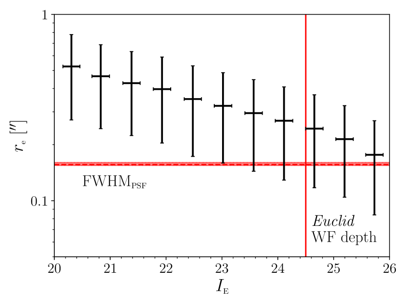
Figure 2: Input magnitude-size distribution of galaxies. The data points are the mean $r_{\text{e}}$ as a function of $I_{\scriptscriptstyle\rm E}$. Also shown are the standard deviation of $r_{\text{e}}$ and $I_{\scriptscriptstyle\rm E}$ in each bin. The horizontal band denotes the PSF FWHM and its variation across the field of view. A significant fraction of the galaxies have intrinsic effective radii similar to the PSF, especially at the Euclid wide field (WF) depth.

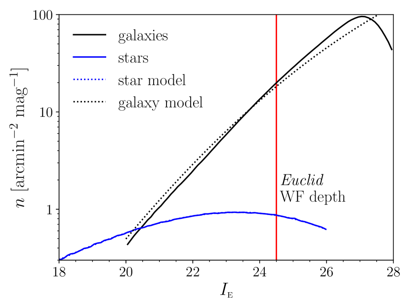
Figure 3: Input differential number count for galaxies and stars. Solid is the measured galaxy count from Flagship. Dashed is a polynomial model of VIS-corrected magnitudes in the GOODS South ($I_{\scriptscriptstyle\rm E}<26$) and Ultra Deep Field ($I_{\scriptscriptstyle\rm E}>26$). Stars are drawn from a polynomial model of $i$ magnitudes generated with the Besançon model in the North Ecliptic Pole. The cumulative number counts are $\qty{250}{arcmin^{-2}}$ ($I_{\scriptscriptstyle\rm E}<29.5$) for galaxies and $\qty{6}{arcmin^{-2}}$ ($I_{\scriptscriptstyle\rm E}<26$) for stars.

We define sky patches of size $380\mathrm{″}$ (about $\qty{40}{arcmin^{2}}$), broadly corresponding to the size of a single Euclid CCD, but also include an adjacent area of extra 10% (called buffer/guard region) all around the patch to draw objects in the image that will not be part of the measurement. When selecting the morphological properties from the Flagship catalogue (ellipticity, disc scale length, bulge fraction, position, and flux), their AB flux is first converted to AB magnitude, then further converted to VIS photoelectron count rate via the magnitude-flux relation of Eq. (29)). We assume a constant magnitude zero-point of $I_{\scriptscriptstyle\rm E,\,0}=25.719$, which has been calculated using Euclid as-designed system throughput data. Star positions are drawn from the count model uniformly in each patch.

All galaxies in each patch have ellipticity assigned by Flagship. In principle we could use the cosmic shear from Flagship, however in this work we apply the same constant shear to all galaxies in a patch, with the shear varying from one patch to another according to a uniform distribution on a circle of radius $|g|=0.02$ and random orientation. This choice mimics the typical shear expected for a real survey and also minimises the error on multiplicative bias. We assume an (infinitely thin) annular distribution as opposed to a disc distribution or an even more realistic log-normal distribution because we want to minimise the statistical error on multiplicative bias, and obviously be as cosmology agnostic as possible. On the other hand, a variable shear field might in principle introduce an additional correlation with neighbour bias, particularly if neighbours at different redshifts are considered (MacCrann et al., 2021). However, capturing realistic clustering is the most important aspect of the simulations, which is what we focus on in this work. Similarly to previous work (Bridle et al., 2010; Kannawadi et al., 2019), we apply shape noise mitigation by making, in total, 4 clones of each patch with all ellipticities rotated by $45^{\circ}$ while maintaining the same overall constant shear, which gives us significant leverage on the required simulation volume. It is worth noting, though, that a varying shear could also be dealt with in a shear response approach, leading to an increased effective sample size and reduce simulation volume in calibration (Pujol et al., 2019; Jansen et al., 2024).

We set up a suite of simulations for each of 9 realisations of the PSF image drawn at different positions in the field of view. While varying the PSF image, we keep the objects at the same positions. We assume a Euclid PSF model for a fixed SBc-type galaxy SED at $z=1$, the median of the distribution. The mean ellipticity and its variation across the field of view is: $\epsilon_{1,\text{PSF}}=0.017^{+0.038}_{-0.024}$ and $\epsilon_{2,\text{PSF}}=0.001^{+0.042}_{-0.020}$, with the superscript and subscript denoting absolute ranges. We note that this variation, if not included in the modelling, would be responsible for an error in the shear measurement that would far exceed science requirements. We do not include PSF mismodelling in our simulations as the current Euclid requirement on PSF ellipticity error is already quite stringent, but will be addressed elsewhere. The Euclid Wide Survey is designed to take 4 dithered exposures (pointings), plus two extra short exposures, of the same sky area. Most often these will be taken in the same observation. Hence the PSF model is not expected to vary too much across the exposures, but the images will be different because taken at different positions in the field of view.

We generate Euclid detector images containing galaxies rendered with the brightness model of Sect. 2.1 with varying ellipticity, $r_{\text{e}}$, position, and fluxes. In our initial tests, we make our results insensitive to model bias by construction, and therefore we fix $n_{\text{b}}$, $r_{\text{h}}/r_{\text{e}}$ and $r_{\max}/r_{\text{e}}$. Later on, we address model bias sensitivity by allowing $n_{\text{b}}$, and $r_{\text{h}}/r_{\text{e}}$ to vary. For stars, we use a restricted model with zero ellipticity and $r_{\text{e}}$, so we effectively render point-like PSF images. For the measurement, we will be using the same galaxy profile (with fixed bulge parameters) for all detected objects.

The pixel photoelectron noise is given by

$$\sigma_{\text{px}}^{2}(x,y)=\left(R_{\text{bkg}}+R_{\text{dark}}\right)\tau+\lambda_{\text{obj}}(x,y)+\sigma_{\text{read}}^{2}\leavevmode\nobreak\ .$$ (30)

The first term is Poisson noise from a constant zodiacal light background and dark current, with rates $R_{\text{bkg}}=\qty{0.225}{e^{-}/s}$ and $R_{\text{dark}}=\qty{0.001}{e^{-}/s}$, and exposure time $\tau=\qty{565}{s}$. The second term, $\lambda_{\text{obj}}(x,y)$, is spatially varying Poisson noise from all the objects in the image, which is non-negligible in the Euclid VIS images. The third term is Gaussian noise from the CCD readout with a constant $\sigma_{\text{read}}=\qty{4.5}{e^{-}}$. We assume that all noise sources are uncorrelated. In generating the images, we also apply a bias of $\qty{2000}{e^{-}}$ (about as expected for Euclid), and finally digitise the data. Digitalisation corresponds to dividing the image by a gain of $\qty{3.1}{e^{-}/ADU}$ and floor truncating it to nearest integer, which itself adds uniform noise of variance $1/12\,\unit{ADU}$. We set a tangent projection as our WCS at the centre of the patch, draw 4 undithered exposures and stack them up by taking their average. These images will be used by the object detection for the main results presented here, but we will also include a discussion about the dithering. An example of stacked CCD image is shown in Fig. 4.

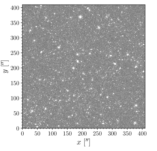
Figure 4: Example of LensMC-Flagship image. The input galaxy distribution is provided by Flagship and stars are drawn from a model. We emulate the VIS detector by including realistic image properties and noise, but we do not include non-linearities, CTI, BFE, or cosmic rays. To aid the visualisation of the faint objects, the image has been clipped between the 10th and 90th percentiles, illustrating the sheer number of objects and their clustering. The image size is 4096 pixels.

4 Results

To quantify the performance of LensMC on our realistic LensMC-Flagship simulations, we run the measurement on about $45\,000$ random patches, which is equivalent to an area of about $\qty{500}{deg^{2}}$, with mean number density, according to Fig. 3, of $\qty{250}{arcmin^{-2}}$ ($I_{\scriptscriptstyle\rm E}<29.5$) for galaxies and $\qty{6}{arcmin^{-2}}$ ($I_{\scriptscriptstyle\rm E}<26$) for stars. We measure the same area (with the objects at the same positions) 9 times for varying noise realisations and PSF across the field of view, totalling an equivalent, effective area of $4500\,\unit{deg^{2}}$. We run all our simulations across the GridPP UK network (Faulkner et al., 2005; Britton et al., 2009). A qualitative test of the measurement performance is shown in Fig. 5. After the galaxy models have been subtracted from the image data, the residuals look consistent with noise, for galaxies measured individually or jointly in groups, despite the presence of neighbours. More quantitative tests will be discussed as part of the validation presented in Appendix C.

	Data	Model(s)	Residuals
One galaxy
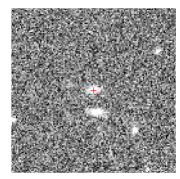
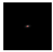
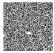
One galaxy
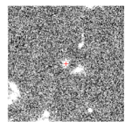
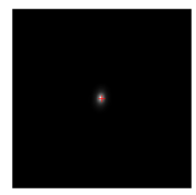
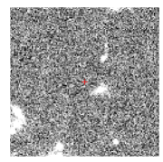
Two galaxies
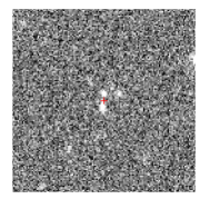
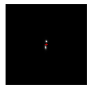
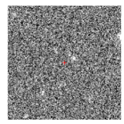
Two galaxies
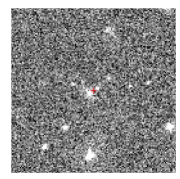
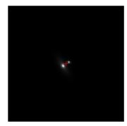
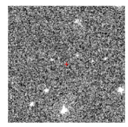
Three galaxies

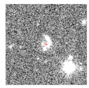
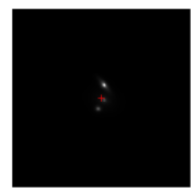
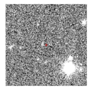
Figure 5: Examples of measurement performance. The target galaxies are denoted with a cross. The image residuals look consistent with noise, for galaxies measured individually or jointly in groups, despite the presence of neighbours. All images have a size of 128 pixels.

4.1 Selection

For our baseline test, we run SourceXtractor++ (Bertin et al., 2020; Kümmel et al., 2020) to detect galaxies and stars in each of the undithered stacked images. The code attempts to deblend detected objects and produces a detection catalogue with a total number density of $\qty{88}{arcmin^{-2}}$ ($I_{\scriptscriptstyle\rm E}<26.5$), and $\qty{34}{arcmin^{-2}}$ ($I_{\scriptscriptstyle\rm E}<24.5$). Figure 6 contains the galaxy magnitude selection applied by SourceXtractor++. This shows the number count of the objects in the simulation and after the detection by SourceXtractor++. The detection catalogue is complete to the magnitudes of interest, apart from false positives of about $\qty{6}{arcmin^{-2}}$ ($I_{\scriptscriptstyle\rm E}<24.5$), probably due to a combination of sub-optimal detection and mismatching with the true input catalogue in presence of neighbours at those magnitudes.

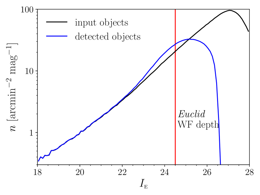
Figure 6: Differential number count for all objects in the simulation and after the detection by SourceXtractor++. The detection catalogue is mostly complete to $I_{\scriptscriptstyle\rm E}<24.5$, apart from false positives of about $\qty{6}{arcmin^{-2}}$ ($I_{\scriptscriptstyle\rm E}<24.5$). The distribution starts rolling off at 26, so a large fraction of faint objects is not detected.

The detections are grouped (with $r_{\text{friend}}=$$$) according to their reported SourceXtractor++ positions. LensMC goes through each object group and measures the object parameters starting from an initial guess at the provided SourceXtractor++ positions. If the size of the group is 1, LensMC will measure the object in isolation and masks out neighbours through the supplied segmentation maps. Instead, if it is greater than 1, LensMC will measure the objects jointly, while masking out neighbours belonging to other groups. We match the input catalogue with the measurement catalogue and within a maximum angular distance of $0.\mathrm{″}3$ from the measured object (which also corresponds to the LensMC maximum search region around the detected object). The few measured objects that do not get a useful match to within that distance are then flagged up and removed from the analysis. We test the sensitivity to the maximum match distance without noticing any appreciable change to the bias.

A key selection applied to the measurement catalogue is the star-galaxy separation. As found in applications to real data, the object size is an excellent statistic to discriminate between galaxies and stars (Sevilla-Noarbe et al., 2018). Therefore we classify objects according to measured $r_{\text{e}}>r_{\text{s/g}}$ where $r_{\text{s/g}}=$$$, which is slightly larger than the pixel size and image resolution. Note that we apply our star-galaxy separation to broadband data simulated with a fixed choice of SED representative of a typical galaxy at redshift 1. However, this does not test how well the star-galaxy separation works with a broad range of galaxy SEDs, and also with a clear distinction between galaxy and star SEDs. We quantify the performance of our separation by calculating: i) $N_{\text{g}}$, the number of true positives, i.e., galaxies correctly identified as such; ii) $N_{\text{s}}$, the number of true negatives, i.e., stars correctly identified as such; iii) $N_{\neg{\text{g}}}$, the number of false positives, i.e., stars wrongly identified as galaxies; iv) $N_{\neg{\text{s}}}$, the number of false negatives, i.e., galaxies wrongly identified as stars. The above numbers are always defined in the measurement catalogue. The true positive rate (TPR) and false positive rate (FPR) are

TPR $$=\frac{N_{\text{g}}}{N_{\text{g}}+N_{\neg{\text{s}}}}\leavevmode\nobreak\ ,$$ (31)

FPR $$=\frac{N_{\neg{\text{g}}}}{N_{\neg{\text{g}}}+N_{\text{s}}}\leavevmode\nobreak\ .$$ (32)

Realistic values of $\text{FPR}>0$ and $\text{TPR}<1$ are always linked to type I and II errors in the shear analysis. Type I is the inclusion of stars in the lensing sample, hence leading to potentially large negative multiplicative bias. Type II is the omission of galaxies (with potentially large shear signal) from the lensing sample which introduces selection bias and also a dilation in statistical error.

For the sample of detected objects to the detection limit ($I_{\scriptscriptstyle\rm E}<26.5$) we find $\text{TPR}=93.3\%$, $\text{FPR}=4.6\%$, purity of 99.8%, and a star fraction of 6.6%. The TPR gives us the frequentist probability of a positive being a galaxy, so $\text{TPR}=p(+|\text{g})$. Similarly, $\text{FPR}=p(+|\text{s})$. Bayesian posterior probabilities provide a more meaningful interpretation of those numbers. The prior probability of an object being a galaxy is $p(\text{g})$ and a star is $p(\text{s})=1-p(\text{g})$ (i.e., the star fraction). Applying Bayes’ theorem we get the probability of a galaxy given a positive detection,

$$p(\text{g}|+)=\frac{p(+|\text{g})\,p(\text{g})}{p(+|\text{g})\,p(\text{g})+p(+|\text{s})\,p(\text{s})}\leavevmode\nobreak\ ,$$ (33)

and similarly for $p(\text{s}|+)$. With the numbers above we obtain $p(\text{g}|+)=99.7\%$ and $p(\text{s}|+)=0.3\%$ for all objects in the detection catalogue. A more relaxed FPR of about $20\%$ would still give us $p(\text{g}|+)=99\%$ and $p(\text{s}|+)=1\%$, given the strong imbalance between the galaxy and star samples. These numbers give us reassurance that once an object has been classified as a galaxy, there is an average $3\,\sigma$ confidence that it will indeed be a galaxy for the entire sample up to the detection limit ($I_{\scriptscriptstyle\rm E}<26.5$).

Figure 7 shows the size distribution of true galaxies and true stars and the operating curve (true positive rate vs false positive rate for varying threshold) of our classification with either a horizontal line or a cross to denote the default threshold, $r_{\text{s/g}}=$$$. Both plots provide solid justification for our choice of $r_{\text{s/g}}$, but confusion is evident around $I_{\scriptscriptstyle\rm E}=24$, which might explain most of the false positives. The area under the operating curve at the bottom of Fig. 7 is large, and the curve itself is reasonably flat for a wide range of false positive rate suggesting excellent discrimination and weak sensitivity on the threshold (in that the shear bias does not appreciably change for a wide range of threshold values around the nominal one). However, in real measurements, an optimal value could be inferred from external data or simulations, hence allowing for a dramatic reduction of the false positives at the expense of a modest reduction in the true positives. Our TPR, FPR, and operating curve of Fig. 7 are consistent or better than the best estimators presented in Sevilla-Noarbe et al. (2018), although a key caveat in our work is likely to be that we have not included a full colour variation of galaxy and star SEDs, which would lead to variable PSFs and potentially harder separation. Moreover, we do not investigate any effect due to star density variation, which might well change by a factor 2 or 3 going from the high to the low latitudes.

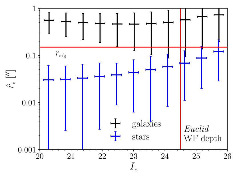
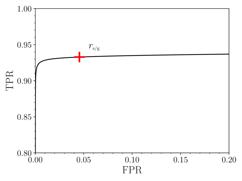
Figure 7: Star-galaxy separation of detected objects. (Top) Observed size-magnitude distribution of true galaxies and stars. The data points are the mean of $r_{\text{e}}$ as a function of $I_{\scriptscriptstyle\rm E}$. Also shown are the standard deviation of $r_{\text{e}}$ and $I_{\scriptscriptstyle\rm E}$ in each bin. $r_{\text{s/g}}=$$$ provides a good separation threshold working up to $I_{\scriptscriptstyle\rm E}<24$. (Bottom) Operating curve showing where our threshold (indicated with a cross) sits in terms of true positives (92.9%) and false positives (4.3%). The area under the operating curve is large, and the curve itself is reasonably flat for a wide range of false positive rate suggesting excellent discrimination and weak sensitivity on the threshold (the shear bias does not appreciably change). In real measurements this could be further optimised through access to external data or simulations.

We define our final shear weight by multiplying Eq. (27) by the step function, $\mathrm{H}(r_{\text{e}}-r_{\text{s/g}})$, and show this as a function of magnitude for detected true galaxies and stars in Fig. 8. As the star weight is systematically lower than the galaxy weight, this drastically reduces the impact of those residual stars (false positives) in the catalogue up to the faint magnitudes.

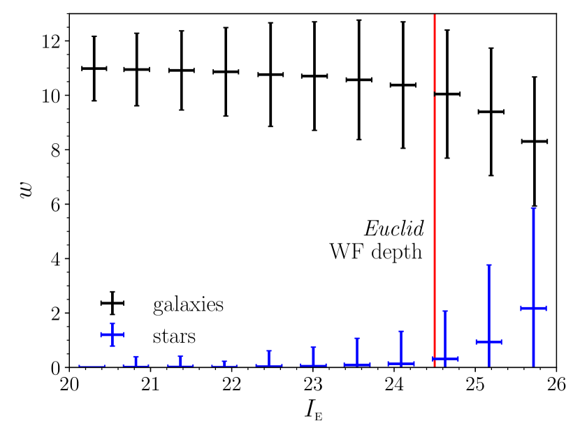
Figure 8: Shear weight after star-galaxy separation of detected objects, as a function of magnitude separately for true galaxies and stars. As the star weight is systematically lower than the galaxy weight, this drastically reduces the impact of those residual stars in the catalogue up to the faint magnitudes.

The quality of our star-galaxy separation can only be tested by fully propagating results through shear bias. We calculate the shear bias for perfect star-galaxy separation (where we enforce knowledge about the truth, i.e., we do not use our classification, but exclude true stars from the galaxy catalogue), and compare it with our nominal analysis. We do not see any statistically significant difference in shear bias between the two cases. Additionally, we vary the value of $r_{\text{s/g}}$ and again find that the bias does not change appreciably.

4.2 Shear bias

As a preliminary validation, Appendix C contains a few distributions and correlations. We test the bias as a function of input true magnitude to avoid large selection biases due to binning by observed quantities, such as S/N or $r_{\text{e}}$, which strongly correlate with shear (Fenech Conti et al., 2017). We define 12 bins in $20<I_{\scriptscriptstyle\rm E}<24.5$ and, in each bin, we regress the measured ellipticity against input true shear via weighted least square as described in detail in Appendix D. We also want to clearly separate measurement (shear measurement method) from purely selection (detection, catalogue matching, weights, and star-galaxy separation) effects. Let $g_{i}$ be the input true shear, $\hat{\epsilon}_{i}$ the measured ellipticity, and $\epsilon_{i,\text{sel}}$ the input true sheared ellipticity on the same selection. Similarly to Eq. (8) where we regress estimates of shear with input true shear, we can define the same regression of our estimate of shear, i.e., ellipticity,

$$\hat{\epsilon}_{i} =(1+m_{i})\,g_{i}+c_{i}+n_{i}\leavevmode\nobreak\ ,$$ (34)

$$\epsilon_{i,\text{sel}} =(1+m_{i,\text{sel}})\,g_{i}+c_{i,\text{sel}}+n_{i,\text{sel}}\leavevmode\nobreak\ ,$$ (35)

where $i=1,2$ indexes the ellipticity or shear component, $n_{i}$ and $n_{i,\text{sel}}$ are the statistical noise components for measurement and selection. The first equation estimates the total of measurement and selection bias, whereas the second one estimates the selection bias. Therefore if we take the difference between the two, and regress $\hat{\epsilon}_{i}-\epsilon_{i,\text{sel}}$ with $g_{i}$,

$$\hat{\epsilon}_{i}-\epsilon_{i,\text{sel}}=m_{i,\text{meas}}\,g_{i}+c_{i,\text{meas}}+n_{i}-n_{i,\text{sel}}\leavevmode\nobreak\ ,$$ (36)

we can then directly estimate the measurement bias, having coherently subtracted the selection bias, and we reduce the statistical noise thanks to the correlation between $n_{i}$ and $n_{i,\text{sel}}$. The measurement-only bias is then defined as $m_{i,\text{meas}}=m_{i}-m_{i,\text{sel}}$ and $c_{i,\text{meas}}=c_{i}-c_{i,\text{sel}}$.

The main performance metric that we present here is the total bias computed as a weighted average over magnitude bins and PSF variation across the field of view as shown in Fig. 9. The performance metric is defined in an $m$-$c$ plane for each of the two components fitted independently. We indicate the Euclid requirements $\sigma_{m}$ and $\sigma_{c}$ in the shaded areas, both the total one and the desired for measurement alone. From looking at the summary figures of Table 2, selection effects are dominating the error budget, with a pronounced asymmetry between the two components. We test that this is not due to the star-galaxy separation, weights, or the particular PSF used here by varying each parameter and checking that results remain consistent with the default analysis. To investigate if the origin of this asymmetry could be due to the input distributions, we estimate the bias of the input ellipticity (before detection) in exactly the same way as we do for our measurements, finding no bias up until the detection is run. We defer the investigation of sensitivity to the SourceXtractor++ configuration to future work. For the time being, we highlight that the multiplicative bias owing to measurement alone (i.e., the shear measurement method) is about $-4\times 10^{-3}$ with an uncertainty of $2\times 10^{-4}$, and a small residual asymmetry in additive bias. All statistical errors for selection and measurement have been estimated following the modelling of Eqs. (34) and the analytical solution presented in Appendix D. The modelling effectively uses the high correlation between measurement and selection estimates to reduce the error on bias. Once selection and measurement biases are calculated, the total bias is just the sum of the two individual values. The total error is then the sum in quadrature, given that the individual values have had their correlation removed.

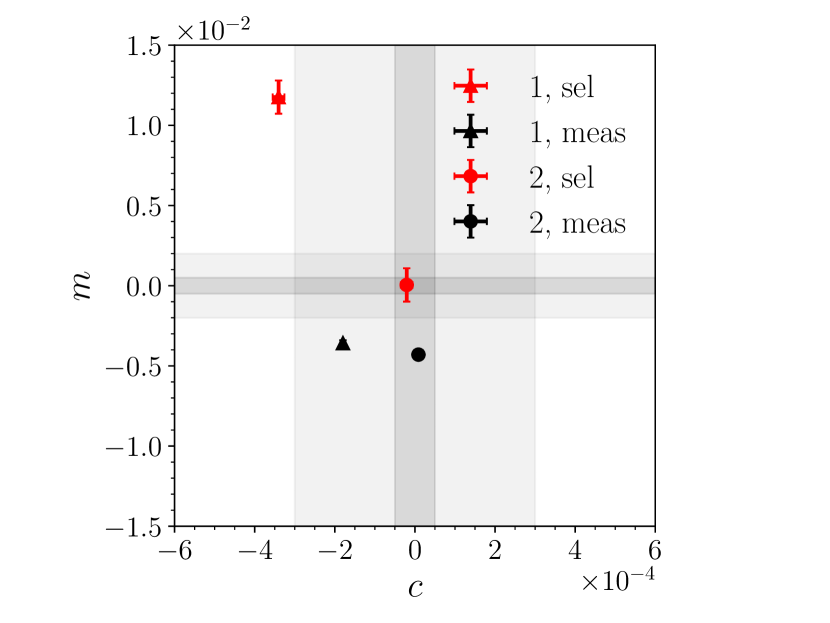
Figure 9: Multiplicative and additive biases averaged over the magnitude selection $20<I_{\scriptscriptstyle\rm E}<24.5$ and PSF variation across the field of view, for measurement and selection. Triangle or circle denote either of the two components. Light shaded area is the Euclid requirement on knowledge of $m$ and $c$, respectively $\sigma_{m}<2\times 10^{-3}$ and $\sigma_{c}<3\times 10^{-4}$. Dark shaded area is the ideal target for measurement alone, respectively $\sigma_{m}<5\times 10^{-4}$ and $\sigma_{c}<5\times 10^{-5}$. Reference values can be found in Table 2.

Table 2: Multiplicative and additive biases averaged over the magnitude selection $20<I_{\scriptscriptstyle\rm E}<24.5$ and PSF variation across the field of view, for measurement and selection (detection, catalogue matching, star-galaxy separation, and weights).

	Measurement	Selection
$m_{1}\,/\,10^{-3}$	$-3.58\,\pm\,0.18$	$11.8\,\pm\,1.0$
$c_{1}\,/\,10^{-4}$	$-1.797\,\pm\,0.025$	$-3.40\,\pm\,0.15$
$m_{2}\,/\,10^{-3}$	$-4.30\,\pm\,0.18$	$0.0\,\pm\,1.0$
$c_{2}\,/\,10^{-4}$	$0.088\,\pm\,0.025$	$-0.21\,\pm\,0.15$

A more in-depth investigation can be carried out when looking at bias as a function of true input magnitude as shown in Fig. 10. As already mentioned, not only is the correlation between magnitude (or flux) with shear negligible (apart from magnification, not included here), but defining true input bins is also essential to minimise the impact of selection bias and not to misinterpret results. Curves are averaged over the PSF variations across the field of view. We note that $m$ and $c$ show a negative trend at the faint magnitudes. This suggests that the total bias shown in Fig. 9 is mostly dominated by those bins, which happen to have the largest relative weight due to the number count increasing with magnitude. The requirement, $\sigma_{m}$ and $\sigma_{c}$, on each bin is derived from the total requirement by increasing the per-bin variance by the decrease in number count in each bin. The error bars are consistent with this.

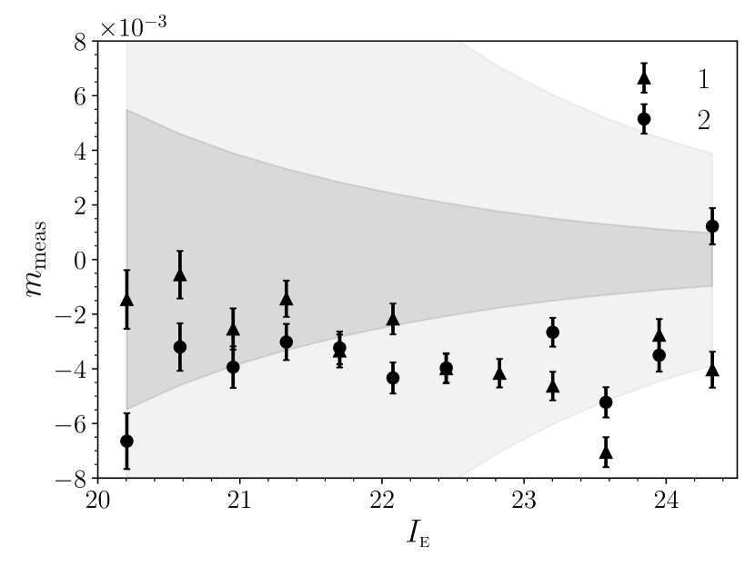
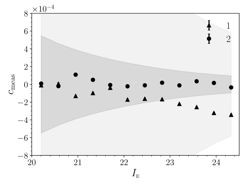
Figure 10: Measurement multiplicative and additive biases in bins of $I_{\scriptscriptstyle\rm E}$ and averaged over the PSF variations across the field of view. Triangle or circle denote either of the two components. Shaded areas are the Euclid requirements relaxed by the increase in variance in each bin. Except for $c_{1,\textrm{meas}}$, which is fully consistent with requirements, all other biases show a slight trend in the faintest bins.

We test the sensitivity to the faint undetected objects by calculating the total bias as a function of the intrinsic limiting magnitude in the simulations. For this we repeatedly render images excluding the faintest objects, with a varying magnitude limit. We expect that the brighter the magnitude limit in the simulation, the weaker the impact of faint objects on the measurement (as their relative fraction becomes small). Figure 11 shows different trends in bias with the magnitude limit. For multiplicative bias, the selection bias seems to be insensitive to the magnitude limit; instead, the measurement bias seems to be symmetric (components are consistent with one another) and shows a trend with the magnitude limit, with a slight hint of flattening out at the faintest end. This effect on the measurement bias indicates a circularisation bias due to the faint objects. Overall, we estimate $m_{\text{faint}}\approx-5\times 10^{-3}$ just due to the presence of faint undetected objects. This is fully consistent with earlier predictions of a few $10^{-3}$ up to $10^{-2}$ depending on the clustering of the faint objects (Euclid Collaboration: Martinet et al., 2019). We think the flattening of the measurement curves with the magnitude limit might be due to the faint galaxies having less impact the fainter they are, or perhaps a lack of an ultra-faint population. However, this indicates that any calibration strategy relying on external images should render galaxies with a magnitude limit of at least 27.5, which is 3 deeper than the Euclid Wide Survey, and the sensitivity to that limit should be investigated as well.

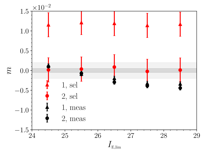
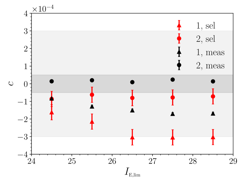
Figure 11: Multiplicative and additive biases for measurement and selection as a function of the intrinsic limiting magnitude in the simulations for a PSF chosen at the centre of the field of view. Triangle or circle denote either of the two components. Shaded areas are the Euclid requirements. The measurement bias shows varying trends with the limiting magnitude, and asymmetries between components in some cases. See text for discussion.

We estimate the bias due to close detected neighbours by comparing results from running the measurement in two modes: $r_{\text{friend}}=0$ or $r_{\text{friend}}=$$$. As discussed in Sect. 2.4, the first mode corresponds to no grouping of detections at all, so LensMC measures all the objects individually, hence relying on the supplied maps to implement the masking of neighbours. In fact, masking provide limited help when the objects are too close to each other: the final ellipticity estimate of the target object will be slightly biased towards the neighbour. Because of the random orientation around the target object, the net effect is a circularisation of the average ellipticity if not corrected for. Instead, the second mode makes groups of objects that are measured jointly. In total, almost 96% of the objects are still measured in isolation, 4% in pairs, and 0.2% in groups that include triplets, quadruplets, and some rare quintuplets. The measurement of the groups increases the robustness to neighbours and mitigates the reliance on the accuracy of the maps at short angular separations between objects. We find a differential multiplicative bias of $m_{\text{neighbour}}\approx-7\times 10^{-4}$ due to the masking of close neighbours (4.2% of the sample) when measuring objects individually ($r_{\text{friend}}=0$), and when joint measuring them in groups ($r_{\text{friend}}=$$$). As the neighbour bias predominantly effects the short separation between objects and the fraction of multiplets compared to the pairs is very small, we expect that increasing $r_{\text{friend}}$ further would provide little benefit to the bias, but at a much increased computational expense.

We also check the dependence of bias on the weight definition of Eq. (27) or the one employed by KiDS (Miller et al., 2013),

$$w_{\scriptscriptstyle\rm KiDS}=\left(\frac{C_{\epsilon}\,\epsilon^{2}_{\max}}{\epsilon^{2}_{\max}-2C_{\epsilon}}+\sigma^{2}_{\epsilon}\right)^{-1},$$ (37)

as a function of the assumed shape noise, $\sigma_{\epsilon}$. We estimate the first-order sensitivity as linear regression to the bias for varying $\sigma_{\epsilon}$. For either definition, we find weak sensitivity: $\text{d}m/\text{d}\sigma_{\epsilon}\approx 4\times 10^{-4}$ and $\text{d}c/\text{d}\sigma_{\epsilon}\lesssim 4\times 10^{-6}$. The implication is such that a change in the assumed $\sigma_{\epsilon}$ of, e.g., 20% would be responsible for an additional bias of order of $10^{-5}$.

Finally, we carry out a test on exposures dithered randomly between $[-0.05,0.05]\,\unit{$\mathrm{\SIUnitSymbolArcsecond}$}$. In reality, the dithering could be as large as a few arcmin, but sampling is always affected by the random sub-pixel shifts. In a real survey, any stacking procedure, even if applied to nominally undithered exposures, will be affected by the random shifts in the telescope pointing at the sub-pixel level. The combination of such exposures will inevitably introduce pixel correlations in the stacked images and PSFs, a problem that would be exacerbated by combining exposures at different epochs. The aim of this test is to verify that the results between dithered exposures and our perfectly undithered exposures (as presented throughout the text) are fully consistent, so to demonstrate that the method will perform well on dithered exposures on real data. However, we do not quantify the impact of stacking in our tests, nor directly assess any benefit from analysing dithered exposures over stacked exposures. For dithered exposures, we resample-coadd the images with SWarp (Bertin et al., 2002), run SourceXtractor++, and remap the segmentation maps back to individual exposures with SWarp. This data is then passed on to LensMC as usual, with the only difference that it now carries out the measurement jointly across exposures. We run the measurement on one of the PSF images at the centre of the field of view and process the catalogues as usual. We find no statistically significant difference in the estimated bias between the two cases of random dithering and perfectly undithered exposures (as used in the main simulations of this paper). This gives us reassurance that the joint measurement of individual exposures would perform well on real data, and also better than stacking because data interpolation would be avoided. However, it also suggests that any undersampling bias is probably below the statistical uncertainty to be seen in these simulations.

4.3 PSF leakage

Having multiple realisations for the spatially varying PSF model allows us to investigate the dependence of bias on the PSF. Figure 12 shows the calculated leakage terms, $\alpha_{1}$ and $\alpha_{2}$, obtained from a linear fit to measured $c$ against input PSF ellipticity. We find $\alpha_{1,\text{sel}}=(-2\,\pm\,3)\times 10^{-3}$ and $\alpha_{2,\text{sel}}=(-8\,\pm\,3)\times 10^{-3}$ for selection and $\alpha_{1,\text{meas}}=(-9\,\pm\,3)\times 10^{-4}$ and $\alpha_{2,\text{meas}}=(2\,\pm\,3)\times 10^{-4}$ for measurement, averaged over all magnitude bins. We note that the measurement leakage is within the empirical requirement derived in Sect. 2, but $\alpha_{2,\text{sel}}$ is clearly not. Combined with the results from the previous section, in particular Table 2, we can observe that the asymmetry in $c$ is most likely due to the PSF having a factor 10 larger first component of ellipticity in detector frame (which in our setup is anti-aligned with world coordinates along right ascension). It is worth adding that the negligible measurement leakage ensures that this residual additive bias is constant across the field of view and hence potentially straightforward to calibrate. However, the same statement would not entirely apply to the selection leakage where a residual term would still complicate the calibration.

Finally, we test the consistency between the measurement curves when assuming perfect star-galaxy separation or not. In fact, the more elliptical the PSF, the larger the residual additive bias, and the harder separating galaxies from stars will be. Due to the intertwining of chromaticity and variation across the field of view of the PSF, we would expect some leakage due to imperfect star-galaxy separation. Luckily, we do not see that the star-galaxy separation may be appreciably impacting our results in our simulations, but we realise this may not be the case with the full chromaticity of real data.

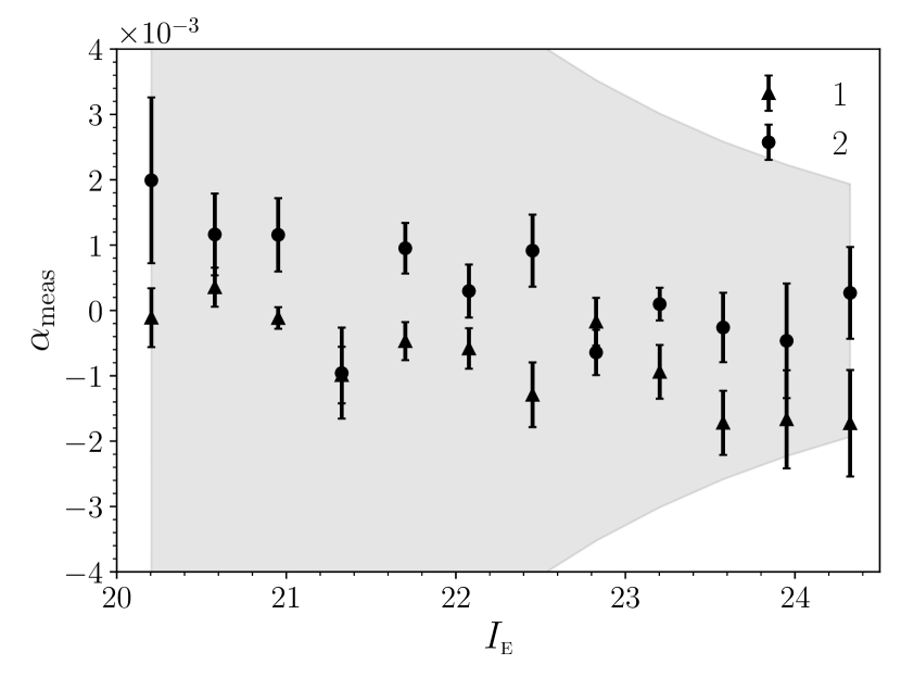
Figure 12: Measurement PSF leakage in bins of $I_{\scriptscriptstyle\rm E}$. Triangle or circle denote either of the two components. Shaded areas are the projected Euclid requirements forward propagated by the corresponding ones on $c$, relaxed by the increase in variance in each bin. The measurement terms are consistent with requirements, except for the first component in the faintest bins.

4.4 Model bias calibration

Having the same galaxy brightness model in both simulations and measurements allows us to isolate the various contributions to the total shear bias, while separating them from the issue of model bias. However, this raises the reasonable concern about whether model bias could be the dominant source of error. Bearing in mind that model bias is usually addressed as part of shear calibration (which is outside of the scope of this paper), we still want to provide reassurance by providing results after we relax some key assumptions made in the previous sections. Then the question of calibratability ties in closely with the sensitivity to the assumptions that are made in the calibration simulations. To address this, the KiDS calibration relies on applying the measurement method to reference simulations and new realisations of the same after having scaled key parameter distributions up and down, with residual biases present in some cases (Li et al., 2023a, b).

Here we choose a similar approach by relaxing some key assumptions in the simulations and then investigate the sensitivity of the calibration. By looking at the list of model parameters in Table 1, we can immediately recognise that the parameters that have been fixed and matched in measurement and simulations take priority. Key parameters are those of the bulges, namely $n_{\text{b}}$ (hence $a_{\text{b}}$) and $r_{\text{h}}$ (hence $r_{\text{h}}/r_{\text{e}}$). Investigating the impact of a distribution of variable bulges to shear bias also makes sense as these are more compact than the discs and not fully captured by LensMC, which always assumes a fixed $r_{\text{h}}/r_{\text{e}}$ in the measurement which could lead to bias. In these tests we allow a broad variation of bulge parameters, shift their distributions up and down as in the KiDS calibration, and see what the impact is on the calibrated shear bias. As part of this tests, we also make some changes to the reference dataset. We select the patches randomly within the available simulation area, simulate objects within a large model array size, and include bulge-only galaxies (accounting for an additional 1% of the galaxies). The last change is required because when allowing the full realism of the bulges, this sub-population of bulge-only galaxies could play a role in model bias. We therefore have the following datasets:

1. a revised reference dataset where the bulge parameters are still being fixed and bulge-only galaxies artificially rendered as two-component galaxies;

2. a new dataset where the bulge parameters are now allowed to vary following a broad distribution of $n_{\text{b}}$ and $r_{\text{h}}$;

3. calibration datasets where the bulge parameters are scaled up and down.

In all cases, during the measurement, LensMC is applied with the same assumptions described earlier in this paper, which allow us to study the differential bias from any assumptions made in the simulations.

While the revised dataset in 1 contains slightly more galaxies, the measurement bias is consistent with results presented in the previous sections. In particular, in this case we find $m_{1,\text{meas}}\approx m_{2,\text{meas}}\approx-3\times 10^{-3}$, $c_{1,\text{meas}}\approx-1\times 10^{-4}$, and $c_{2,\text{meas}}\approx-2\times 10^{-5}$ (cp. with Table 2). However, the selection bias now shows a less pronounced asymmetry between the two components: $m_{1,\text{sel}}\approx 7\times 10^{-3}$, and $m_{2,\text{sel}}\approx 1\times 10^{-2}$, suggesting a possible sensitivity to the changes introduces in the revised dataset in 1. We hypothesise that one of the three changes included in the revised dataset could be playing a role (random patches, larger model array size, and included sub-population), but we defer the study to a future work since the property of the selection bias seems to depend on the details of the image simulation. After running the measurement on dataset 2 and by comparing it with 1, we see the emergence of a model bias $m_{\text{model}}\approx-8\times 10^{-3}$ due to the sub-population of bulge-only galaxies and the full variability of bulges ($n_{\text{b}}$ and $r_{\text{h}}$), now included in the simulations but not captured in the measurement.

This additional bias would be corrected through direct calibration via realistic image simulations. However, it remains to be seen how sensitive the calibration would be to choices made about the bulges in the calibration datasets. This is the main idea behind setting up the new simulations in 3, with distributions that have been scaled up and down to quantify the sensitivity. The top row of Fig. 13 shows the distributions of simulations in 2 and scaled distributions of $n_{\text{b}}$ and $r_{\text{h}}$ in 3. As clarified above, the bulges are always allowed to vary in the simulations, but are not fully captured by the measurement (since LensMC fixes both parameters to their nominal values as in Table 1). These distributions have been scaled up and down by $\pm 20\%$, which is about $30\,\sigma$ away from the mean, comfortably outside the statistical uncertainty of the mean. The following rows of Fig. 13 show the sensitivity of the corrected multiplicative and additive biases to the variation in the scaled calibration dataset. These are shown separately for selection and measurement biases. While the evidence of sensitivity of selection bias is weak due to the large error bars, we do see some sensitivity particularly of measurement multiplicative bias on $r_{\text{h}}$. This is important as knowing the distribution of bulge sizes is essential for an accurate calibration of the bias. We estimate: $\text{d}m_{1,\text{meas}}/\text{d}[\Delta n_{\text{b}}/n_{\text{b}}]\approx-7\times 10^{-4}$, $\text{d}m_{2,\text{meas}}/\text{d}[\Delta n_{\text{b}}/n_{\text{b}}]\approx 4\times 10^{-6}$, $\text{d}m_{1,\text{meas}}/\text{d}[\Delta r_{\text{h}}/r_{\text{h}}]\approx-8\times 10^{-3}$, $\text{d}m_{2,\text{meas}}/\text{d}[\Delta r_{\text{h}}/r_{\text{h}}]\approx-9\times 10^{-3}$. For instance, that would imply a level of bias of $\approx-1\times 10^{-4}$ for every (positive) percent variation on $r_{h}$ assumed in the calibration dataset. Conversely, a bias requirement of, e.g., $1\times 10^{-3}$ would imply a calibration requirement on $r_{h}$ of 10%.

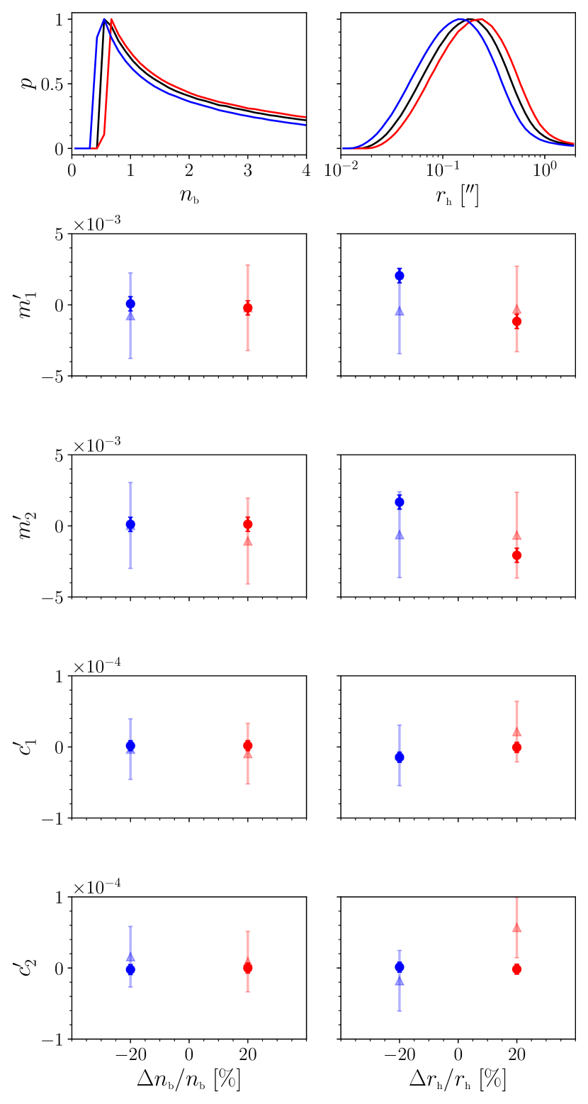
Figure 13: Bias calibration sensitivity. (Top row) Distributions of bulge parameters scaled up and down by $\pm 20\%$ relative to the nominal one at the centre. (Following rows) Calibrated bias using the simulations with scaled bulge parameters. Semi-transparent triangles are selection biases; circles are measurement biases.

While the results presented in this section provides some reassurance that the bias is stable and the sensitivity of the calibration is under control, it is worth mentioning that the variability in bulge distributions included here does not fully capture the variability observed in real data, with realistic morphologies of faint galaxies potentially playing a major role in the Euclid analysis (Csizi et al., in prep.).

5 Summary and discussion

LensMC is our advanced cosmic shear measurement method based on galaxy forward modelling and MCMC sampling that is being developed for Euclid and Stage-IV surveys. We have discussed the key components of the measurement and how to handle real data problems robustly. Its performance has been demonstrated on a suite of suitably complex images, our LensMC-Flagship simulations, which take the Flagship catalogue as input to produce full Euclid-like detector images, including realistic galaxy properties and clustering to $I_{\scriptscriptstyle\rm E}<29.5$, and stars to $I_{\scriptscriptstyle\rm E}<26$. Emulations of the VIS images have been made to include realistic pixel noise and a broadband, chromatic PSF model with spatial variation across the field of view. SourceXtractor++ has been run to detect objects down to $I_{\scriptscriptstyle\rm E}<26$, and LensMC has used segmentation maps to mask out objects, if not belonging to the same group, or jointly measured all objects within the same group.

The bias can be broken down into measurement (from running the method on the detected objects) and selection (detection, catalogue matching, star-galaxy separation, and weights). From Table 2, the selection accounts for a bias of $m_{1,\text{sel}}=(12\pm 1)\times 10^{-3}$, $m_{2,\text{sel}}=(0\pm 1)\times 10^{-3}$, $c_{1,\text{sel}}=(-3.4\pm 0.2)\times 10^{-4}$, and $c_{2,\text{sel}}=(-0.2\pm 0.2)\times 10^{-4}$. Instead, the measurement accounts for a bias of $m_{1,\text{meas}}=(-3.6\pm 0.2)\times 10^{-3}$, $m_{2,\text{meas}}=(-4.3\pm 0.2)\times 10^{-3}$, $c_{1,\text{meas}}=(-1.80\pm 0.03)\times 10^{-4}$, and $c_{2,\text{meas}}=(0.09\pm 0.03)\times 10^{-4}$. The measurement bias would be larger by an additional multiplicative bias of $-7\times 10^{-4}$ if detected objects were not measured jointly. This alleviates the need of having extremely accurate deblended segmentation maps that are usually needed for masking out detected neighbours at a close angular separation. Undetected faint objects remain buried in the noise, and we estimate their multiplicative bias to $-5\times 10^{-3}$. Therefore the measurement bias is dominated by the faint objects and to some extent by the measurement method. We test the sensitivity to other effects, including the star-galaxy separation or the weight definition, but do not find any statistical significance. The leakage due to the PSF variation across the field of view is found to be limited by selection, with the measurement contribution mostly consistent with requirements. Our total $m$ and $c$ biases are to large extent limited by selection and secondarily by the presence of faint objects. First, the detection bias might be improved with an optimisation of detection parameters, e.g.  by a better choice of the SourceXtractor++ convolution filter that should match the PSF size as closely as possible. Second, as the faint objects account for the other largest source of bias after selection, we aim to study the sensitivity on the choice of that distribution by adding an ultra-faint population. Since the bias can be measured from varying the magnitude limit in the input simulations, the differential bias between a shallow and deep limit yields the calibration coefficient required for the correction of the effect due to the faint objects, which is $m_{\text{faint}}=(-5.0\pm 0.2)\times 10^{-3}$. Once simulation complexity is increased after the inclusion of full variability in bulges parameters and bulge-only galaxies, we see the emergence of a model bias $m_{\text{model}}\approx-8\times 10^{-3}$. As this is not captured in the measurement, it is usually corrected as part of the shear bias calibration. In this case, we study the sensitivity of our calibration on assumptions made about the bulges in the calibration datasets, finding that it is modest overall (with a bias of $\approx 1\times 10^{-4}$ for every percent variation in bulge sizes assumed in the calibration dataset). As part of this investigation, we have revisited the datasets and have found a change in the selection bias with a less pronounced asymmetry and smaller magnitude suggesting that the details of the simulation setup may be playing a key role. We defer further study of the selection bias following a further upgrade of the simulations in future work. We find that breaking down the bias into leading effects as shown in this work proves itself as a useful tool when deriving the calibration corrections required for real data applications.

We recognise that our simulations will need further elements of realism. First, we have shown initial results for nominal simulation settings and have studied the sensitivity to some key parameters. This proves essential in order to break down the bias in its main contributions, but it does not give us an exhaustive answer to the full calibratability of our method. While we have tested the sensitivity to some key effects, we will need to carry out a more thorough study of the sensitivity to choices made in SourceXtractor++ (e.g., detection thresholds and convolution filter) and the distribution of faint galaxies. Furthermore, we have shown results for models that match those in the simulations for three parameters (see fixed ones in Table 1) and then also after relaxing assumptions made for bulges. The residual bias is still under control and its sensitivity is weak, but more parameters will need to be varied in a follow-up work. Another point of future work is the inclusion of cosmic rays, which are identified as one of the main causes of concern for space-base lensing surveys. In fact, while these are usually masked out at detector level, residuals and undetected cosmic rays may still impact the shear measurement significantly. Similarly, detector non-linearities, CTI, and BFE have not been included and while again there are already strategies to correct for those at detector level, residuals should still be fully propagated through. A complete study of redshift dependent biases is a further essential step, where it will also be necessary to account for the colour dependence (leading to an effective redshift dependence) of the PSF modelling. As the PSF modelling is a strong function of both colour and redshift, future realistic simulations that include tomographic binning will also have to include the full spatial and colour variability of the galaxies. Closely related, galaxy colour gradients might lead to additional redshift-dependent biases (Semboloni et al., 2013; Er et al., 2018).

Furthermore, our work has so far concentrated on weak lensing shear bias for the cosmic shear using $|g|=0.02$. Euclid will also provide lensing measurements for galaxy clusters, where very massive systems feature reduced shears $|g|>0.1$ even outside the core region (e.g., Schrabback et al., 2018). In this regime non-linear shear responses and increased blending can affect shear calibrations at the percent level (e.g., Hernández-Martín et al., 2020). This must be accounted for in order to reach the accuracy requirements of next-generation cluster cosmology analyses (e.g., Grandis et al., 2019). We therefore additionally plan to conduct dedicated analyses of LensMC using cluster field image simulations, anticipating that ongoing preliminary tests already demonstrate linearity of the method up to $|g|=0.1$.

While our simulations are already up to the standard of the most recent shear measurement simulations, the goal of this paper has been to set up suitably complex simulations that can prove the robustness and performance of LensMC to real-data scenarios, so we are confident about its application to real Euclid data. The added benefit of our simulations is the relative flexibility in the possibility to incorporate and study new effects individually, and the shear bias be broken down into individual effects. This is something that has not been possible with the fully-fledged simulations implemented in the Euclid science ground segment.

We have shown results that have been derived without resorting to external calibration and will demonstrate the full calibratability in a separate paper investigating further realism and sensitivity in much more detail. to summarise, key points of our measurement and why we think this is best for real data are: (i) forward modelling to deal with Euclid image undersampling and convolution by a PSF with comparable size to the many galaxies; (ii) joint measurement of object groups to correctly handle neighbour bias; (iii) masking out objects belonging to different groups; (iv) MCMC to sample the posterior in a multi-dimensional parameter space, which provides shear weights, and correct marginalisation of ellipticity over nuisance parameters and other objects in the same group.

The main findings and takeaways can be summarised as follows. When model bias, chromaticity, and selection biases are suppressed, the obtained biases are close to Euclid requirement. This measurement bias is largely dominated by undetected faint galaxies in the images. The bias is also found to be stable and mostly insensitive to the many effects in the simulations, which we have explored in detail. As the Euclid analysis will also need to correct for other artefacts in the images, because of its stability, the residual bias will be straightforward to calibrate through image simulations. Once we include the model bias in the simulations, the overall bias is found to be significant. However, since the sensitivity is weak, it will be straightforward to also calibrate the model bias through the same image simulations.

Appendix A Likelihood

We wish to linearly marginalise the likelihood in Eq. (17) over flux parameters, $\phi_{i}$. Taking the derivative and equating to zero, we have

$$\frac{\partial}{\partial\phi_{i}}\ln p(\boldsymbol{D}|\epsilon,\theta,\phi)\propto\boldsymbol{I}_{i}(\epsilon,\theta)^{\top}\mathsf{C}^{-1}\Big{[}\boldsymbol{D}-\phi_{j}\boldsymbol{I}_{j}(\epsilon,\theta)\Big{]}=0\leavevmode\nobreak\ ,$$ (38)

where $\boldsymbol{I}_{i}=\partial\boldsymbol{I}/\partial\phi_{i}$. For a linear model, marginalising is equivalent to solving the equation in a least square sense. The Fisher matrix of the problem is defined by the derivatives of the likelihood and is given by Eq. (19). The least square solution is therefore

$$\hat{\phi}_{i}(\epsilon,\theta)=\mathcal{F}^{-1}_{ij}(\epsilon,\theta)\,\rho_{j}(\epsilon,\theta)\leavevmode\nobreak\ .$$ (39)

where $\rho_{j}(\epsilon,\theta)=\boldsymbol{D}^{\top}\mathsf{C}^{-1}\boldsymbol{I}_{j}(\epsilon,\theta)$. The marginal likelihood is found by plugging the solution above into the original likelihood of Eq. (17). This partial marginalisation technique is customary in many fields including cosmology (Taylor & Kitching, 2010), and gravitational wave analysis (Congedo, 2015).

The problem is invertible whenever the Fisher matrix is full rank, $|\mathcal{F}_{ij}(\epsilon,\theta)|>0$. The following two conditions must be satisfied: (i) bulge and disc components must not be the same to avoid degeneracy built in the modelling; (ii) both components must not go to zero. If we were to naively apply the linear solution of Eq. (39) to very faint galaxies, we would often get negative fluxes. This is undesirable, hence we adopt the non-negative least square implementation of Lawson & Hanson (1995). Effectively this is equivalent to the standard least square while enforcing a hard constraint on fluxes, $\phi_{i}>0$. Whenever one of the two fluxes is zero, we make the likelihood collapse to single component modelling. The Fisher matrix of the $i$-th component is now a scalar,

$$\mathcal{F}_{ii}(\epsilon,\theta)=\boldsymbol{I}_{i}(\epsilon,\theta)^{\top}\mathsf{C}^{-1}\boldsymbol{I}_{i}(\epsilon,\theta)\leavevmode\nobreak\ .$$ (40)

The linear solution is

$$\hat{\phi}_{i}(\epsilon,\theta)=\frac{\rho_{i}(\epsilon,\theta)}{\mathcal{F}_{ii}(\epsilon,\theta)}\leavevmode\nobreak\ ,$$ (41)

and the marginalised likelihood is given by

$$\ln p(\boldsymbol{D}|\epsilon,\theta)\propto\frac{1}{2}\frac{\rho_{i}^{2}(\epsilon,\theta)}{\mathcal{F}_{ii}(\epsilon,\theta)}\leavevmode\nobreak\ .$$ (42)

Note that this is just a particular case of the more general Eq. (18), which is valid for more than one model component.

Appendix B MCMC convergence

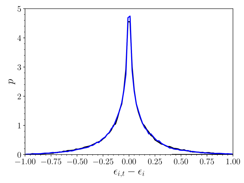
Figure 14: Distribution of shifts of ellipticity components from the truth, marginalised over nuisance for a variety of galaxies. $\epsilon_{i,t}$ is a chain for an ellipticity component with $i=1,2$ and MCMC sample $t$; $\epsilon_{i}$ is the corresponding true value. The distribution peaks at zero, but shows large random values that are usually washed out by taking averages over large samples.

We quantify the average convergence property by calculating the shifts of every MCMC sample from the truth. Fig. 14 shows the distribution of ellipticity component shifts, marginalised over nuisance, for a variety of galaxies of broad morphological properties as described in Sect. 3. This distribution peaks at zero but also shows some large random shifts from the truth. Any such large shift is usually washed out by taking averages over large samples, as it is the case for cosmic shear analyses.

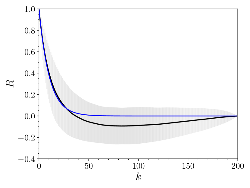
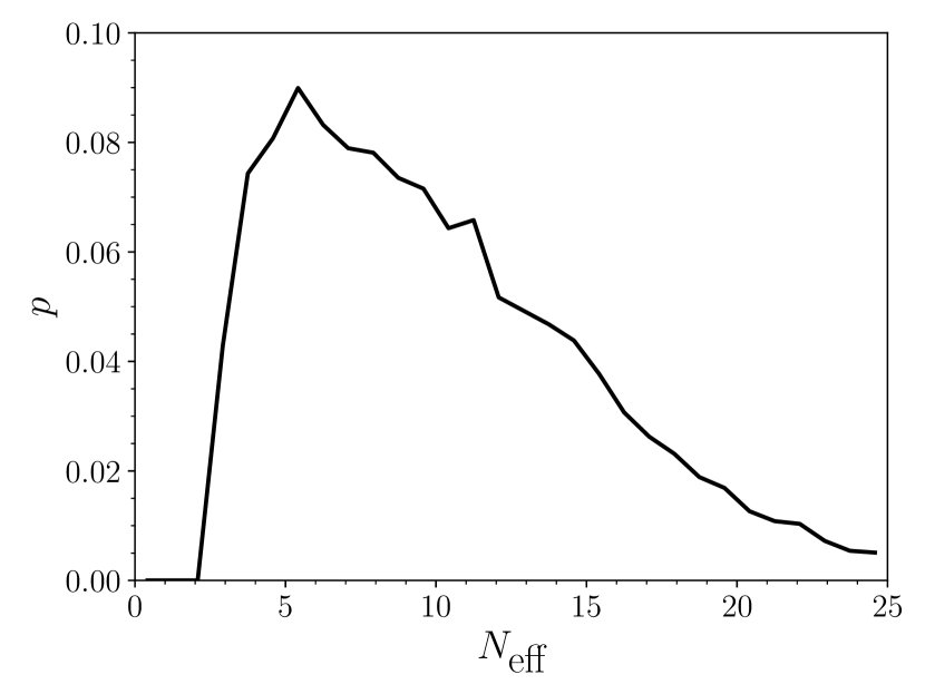
Figure 15: (Top) Sample autocorrelation function of the same ellipticity chains as shown in Fig. 14. The function dies off rapidly approximately as an exponential decay (shown as the analytic curve without error bands) with the same autocorrelation time. A small negative correlation at large lags is an indicator of fast convergence. (Bottom) Distribution of effective sample size for the same chains, whose mean is at about 14 (compare with $N_{\scriptscriptstyle\rm MC}=200$).

A complementary test of convergence is through the analysis of the autocorrelation function. Suppose we have a chain for a generic parameter, $\vartheta_{t}$, with mean $\bar{\vartheta}$ and standard deviation $\hat{\sigma}_{\vartheta}$. The sample autocorrelation function is defined as

$$R_{k}=\frac{1}{\sigma_{\vartheta}^{2}\,(N_{\scriptscriptstyle\rm MC}-k)}\sum_{t}(\vartheta_{t+k}-\bar{\vartheta})\,(\vartheta_{t}-\bar{\vartheta})\leavevmode\nobreak\ ,$$ (43)

where $t=0,\dots,N_{\scriptscriptstyle\rm MC}-k-1$ and $N_{\scriptscriptstyle\rm MC}$ is the chain length. The autocorrelation time quantifies how long the samples will be correlated for, and is given by

$$\tau=1+2\sum_{k}R_{k}\leavevmode\nobreak\ ,$$ (44)

for $k=1,\dots,M$ and $M$ is a cut-off point set by $R_{k-1}+R_{k}<0$ (Geyer, 1992). This truncation is usually required to avoid the inclusion of too much noise at large lags. The top of Fig. 15 shows the mean autocorrelation function of the same ellipticity chains. The 1-$\sigma$ error bars are due to the random variation in the sample. At small lags, the mean autocorrelation function approximately follows an $\exp(-2\,k/\tau)$ trend, and becomes slightly negative at large lags. Positive autocorrelation at large lags is an unwanted feature of any MCMC method as this suggests poor convergence. In contrast, a small negative autocorrelation as shown here suggests faster convergence. This can be seen from, e.g., the estimator of Eq. (44): if $R_{k}<0$ consistently for some $k>0$, the final estimate of $\tau$ would be reduced compared to the case of positive autocorrelation. However, as discussed above, at large lags, the impact of noise on the estimator will be important. To account for autocorrelation in the chain, the sample variance needs to be rescaled by $\tau$, so it is worth introducing the effective sample size as follows,

$$N_{\text{eff}}=\frac{N_{\scriptscriptstyle\rm MC}}{\tau}\leavevmode\nobreak\ .$$ (45)

The distribution of this quantity is shown at the bottom of Fig. 15, and its mean is at about 14 (compare with $N_{\scriptscriptstyle\rm MC}=200$) with a positive skewness towards the larger values. In this context, a large effective sample size is a good indicator of the quality of the chains. In fact, since the MC noise scales as $N_{\text{eff}}^{-1/2}$, a galaxy with typical measurement ellipticity noise of 0.3 will be affected, on average, by a sampling noise of 0.08. Both the intrinsic ellipticity dispersion and sampling noise are diluted by the average over large samples. As the averaged shear will include both noise components, the sampling noise will always be a factor 4 smaller than the intrinsic dispersion. However, in general, one would expect that many more sources of noise may be present in the measurement from image detection to shear, so the sampling term would be expected to be significantly smaller than the total noise.

Appendix C Validation

Fig. 16 shows the distribution of $\chi^{2}/\nu$ for all galaxies in the measurement, where $\chi^{2}=-2\ln p$, $p$ is the likelihood calculated at the mean estimate, and $\nu$ is the number of degrees of freedom. This distribution is broadly consistent with 1, except for a small shift of about 0.15 and a slightly positive skewness. There are likely two reasons for this small shift. The first one could be due to residual features in the data due to inaccurate masking and the presence of undetected faint objects. The second one, more general, is due to the fact that we calculate the $\chi^{2}$ at the mean, not the maximum, and therefore a positive shift should always be expected. In our simulations, we find $\Delta\chi^{2}/\nu\approx 0.015$.

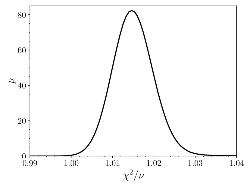
Figure 16: Distribution of $\chi^{2}/\nu$ values. A shift of about 0.15 as well as a slightly positive skewness can be seen in the distribution.

Fig. 17 shows the input-output ellipticity correlation for all the selected galaxies in the catalogue (see discussion about selection in Sect. 4.1), split in three magnitude bins: relatively bright, faint, and very faint. The measured ellipticity correlates very accurately with the true input value. However, as the galaxies become fainter, we observe an increase of noise and a negative bias (which is a reflection of what will be noted about shear in Sect. 4.2). We quantify this bias as the deviation from the perfect correlation line in each of the three magnitude bins: $(1\pm 7)\times 10^{-4}$, $(-2\pm 1)\times 10^{-3}$, and $(-13.0\pm 0.6)\times 10^{-2}$.

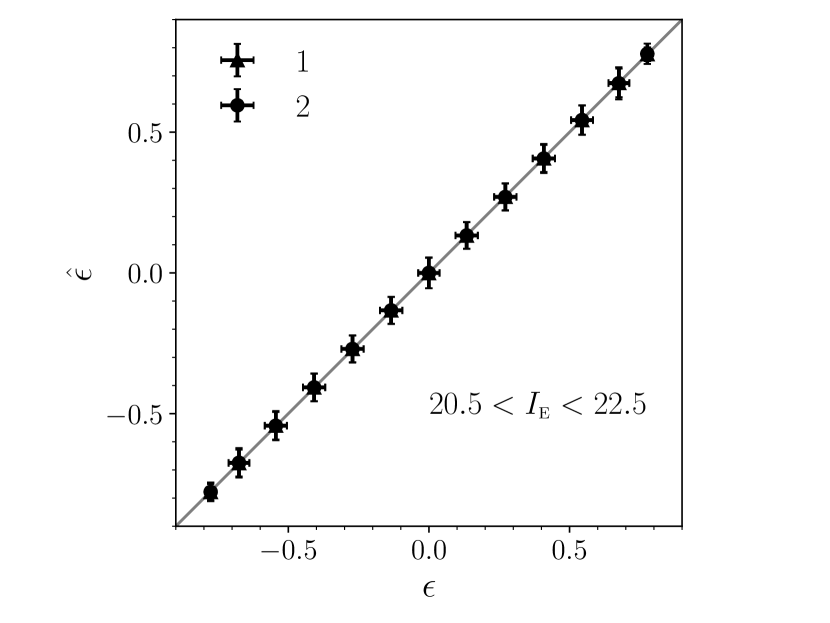
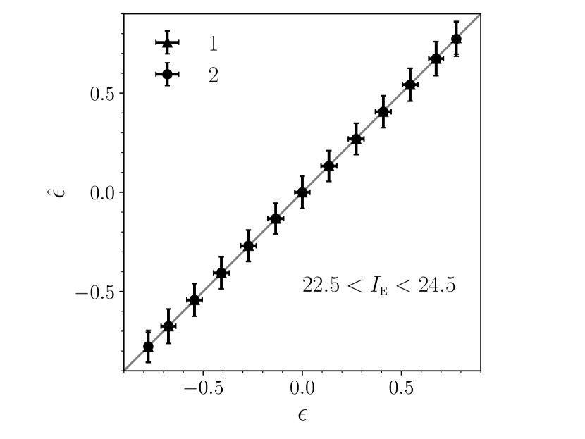
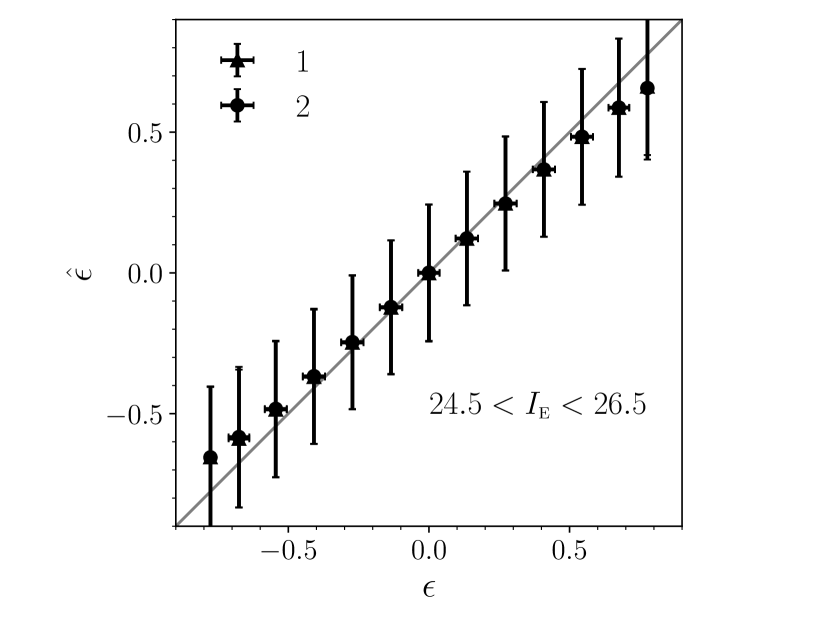
Figure 17: Input-output ellipticity correlation. The correlation has been calculated for the selected sample of galaxies for a relatively bright (top), faint (middle), and very faint (bottom) magnitude bins. The measured ellipticity shows increased noise and a negative bias at the faint end, highlighted as the deviation from the perfect correlation line.

Finally, Fig. 18 shows input-output magnitude and size correlation. The measured magnitude correlates very accurately with the true input value, except at the very faint end. However, the interpretation of the size correlation is a bit more difficult. The small sizes ($r_{\text{e}}<0.25$), comparable with the PSF, are biased high due to the faintness of the galaxies and the poor constraint from the posterior which does not incorporate a realistic size prior. Residual PSF errors are also expected to bias high the sizes. Additionally, a possible leakage from stars might make the situation worse (as discussed in Sect. 4.1). The issue is reversed for the large sizes ($r_{\text{e}}>1.8$), which are biased low. In this case, the galaxies are very bright and their brightness profile extends to very large radii, with a large variation in brightness from the peak to the tail of the distribution. Indeed it is generally hard to measure these objects due to under-modelling of the faint tails. Either way, the impact on lensing is negligible because small, faint galaxies tend to have systematically smaller shear weight (see Fig. 8), while large, bright galaxies are small in number and carry negligible shear signal.

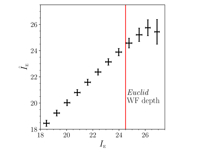
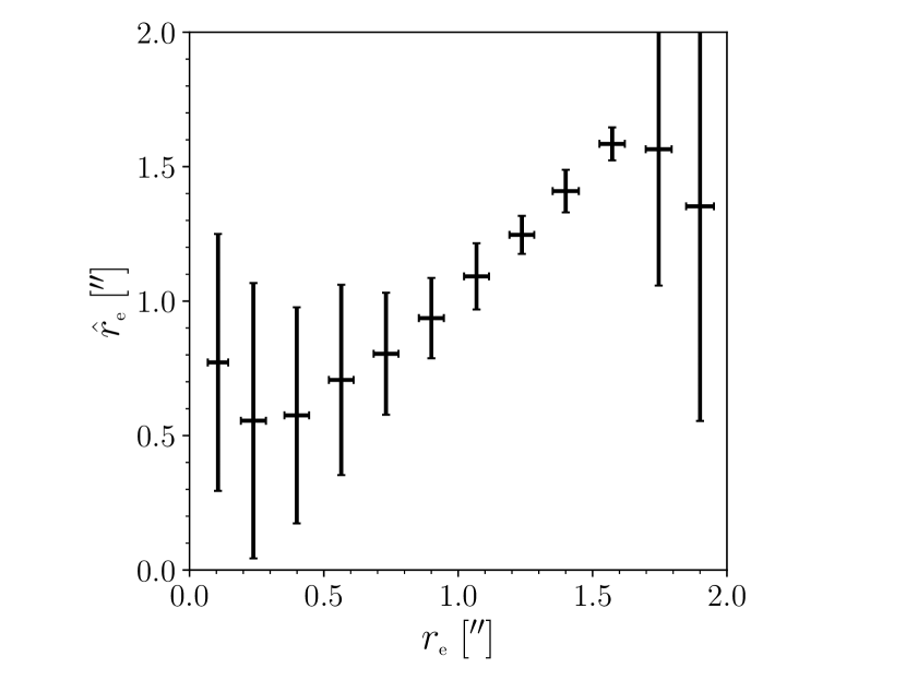
Figure 18: Input-output correlation for magnitude and size. (Top) The magnitude correlation shows a slightly negative bias for very faint galaxies. (Bottom) The size correlation shows positive bias for small sizes and negative bias for large sizes.

Appendix D Shear bias estimate

We wish to derive a maximum likelihood estimator for the bias model of Eq. (8). We aim to regress values for measured ellipticity, $\hat{\epsilon}$, against input shear, $g$, with weights $w$ (not necessarily inverse variance). The corresponding data vectors are denoted as $\boldsymbol{\hat{\epsilon}}$ and $\boldsymbol{g}$, and the weights are assumed to be uncorrelated as a diagonal matrix $\mathsf{w}$. All data vectors and matrices are of the same size $N_{\text{data}}$. The solution $\boldsymbol{\mu}=(m,c)$ is found in least square sense,

$$\hat{\boldsymbol{\mu}}=\mathsf{F}^{-1}\left[(\boldsymbol{\hat{\epsilon}}-\boldsymbol{g})^{\top}\mathsf{w}\,\boldsymbol{J}\right]\leavevmode\nobreak\ ,$$ (46)

where $\mathsf{J}=(\boldsymbol{g},\boldsymbol{1})$ is the Jacobian matrix of size $N_{\text{data}}\times 2$. We assume matrix multiplication throughout and diagonal weights. The Fisher matrix is given by

$$\mathsf{F}=\mathsf{J}^{\top}\mathsf{w}\,\mathsf{J}\leavevmode\nobreak\ ,$$ (47)

which leads to the variance on our estimate,

$$\mathsf{C_{\mu}}=\frac{\chi^{2}}{\nu}\mathsf{F}^{-1}\leavevmode\nobreak\ ,$$ (48)

where $\chi^{2}/\nu$ is the rms of the fit residuals.

The explicit solution (in data index $\alpha$) is as follows

$$\hat{m} =\frac{\sum_{\alpha}w_{\alpha}\delta g_{\alpha}g_{\alpha}\sum_{\alpha}w_{\alpha}-\sum_{\alpha}w_{\alpha}\delta g_{\alpha}\sum_{\alpha}w_{\alpha}g_{\alpha}}{\delta}\leavevmode\nobreak\ ,$$ (49)

$$\hat{c} =\frac{\sum_{\alpha}w_{\alpha}\delta g_{\alpha}\sum_{\alpha}w_{\alpha}g_{\alpha}^{2}-\sum_{\alpha}w_{\alpha}\delta g_{\alpha}g_{\alpha}\sum_{\alpha}w_{\alpha}g_{\alpha}}{\delta}\leavevmode\nobreak\ ,$$ (50)

where $\delta=\sum_{\alpha}w_{\alpha}g_{\alpha}^{2}\sum_{\alpha}w_{\alpha}-\left(\sum_{\alpha}w_{\alpha}g_{\alpha}\right)^{2}$, $\delta g_{\alpha}=\hat{\epsilon}_{\alpha}-g_{\alpha}$. The variance on $m$ and $c$ are given by

$$\sigma_{m}^{2} =\frac{\chi^{2}}{\nu}\frac{\sum_{\alpha}w_{\alpha}}{\delta}\leavevmode\nobreak\ ,$$ (51)

$$\sigma_{c}^{2} =\frac{\chi^{2}}{\nu}\frac{\sum_{\alpha}w_{\alpha}g_{\alpha}^{2}}{\delta}\leavevmode\nobreak\ ,$$ (52)

where $\chi^{2}=\sum_{\alpha}w_{\alpha}(\delta g_{\alpha}-\hat{m}\,g_{\alpha}-\hat{c})^{2}$ and $\nu=N_{\text{data}}-2$.

References

- Abbott et al. (2018a) Abbott, T. M. C., Abdalla, F. B., Alarcon, A., et al. 2018a, Phys. Rev. D, 98, 043526
- Abbott et al. (2018b) Abbott, T. M. C., Abdalla, F. B., Allam, S., et al. 2018b, ApJS, 239, 18
- Abbott et al. (2023) Abbott, T. M. C., Aguena, M., Alarcon, A., et al. 2023, Open J. of Astrophysics, 6
- Aghanim et al. (2020) Aghanim, N., Akrami, Y., Ashdown, M., et al. 2020, A&A, 641, A6
- Aihara et al. (2017) Aihara, H., Armstrong, R., Bickerton, S., et al. 2017, PASJ, 70
- Amendola et al. (2018) Amendola, L., Appleby, S., Avgoustidis, A., et al. 2018, Living Rev. Relativ., 21, 2
- Amon et al. (2022) Amon, A., Gruen, D., Troxel, M. A., et al. 2022, Phys. Rev. D, 105, 023514
- Antilogus et al. (2014) Antilogus, P., Astier, P., Doherty, P., Guyonnet, A., & Regnault, N. 2014, JINST, 9, C03048
- Arcelin et al. (2020) Arcelin, B., Doux, C., Aubourg, E., Roucelle, C., & Collaboration), T. L. D. E. S. 2020, MNRAS, 500, 531
- Asgari et al. (2021) Asgari, M., Lin, C.-A., Joachimi, B., et al. 2021, A&A, 645, A104
- Bauer et al. (2015) Bauer, D., Colling, D., Currie, R., et al. 2015, J. Phys. Conf. Ser., 664, 062036
- Beckwith et al. (2006) Beckwith, S. V. W., Stiavelli, M., Koekemoer, A. M., et al. 2006, ApJ, 132, 1729
- Behnel et al. (2011) Behnel, S., Bradshaw, R., Citro, C., et al. 2011, Comput. Sci. Eng., 13, 31
- Bernstein (2010) Bernstein, G. M. 2010, MNRAS, 406, 2793
- Bernstein & Armstrong (2014) Bernstein, G. M. & Armstrong, R. 2014, MNRAS, 438, 1880
- Bernstein et al. (2016) Bernstein, G. M., Armstrong, R., Krawiec, C., & March, M. C. 2016, MNRAS, 459, 4467
- Bertin et al. (2002) Bertin, E., Mellier, Y., Radovich, M., et al. 2002, 281, 228
- Bertin et al. (2020) Bertin, E., Schefer, M., Apostolakos, N., et al. 2020, ASPCS, 527, 461
- Betancourt (2017) Betancourt, M. 2017, arXiv:1701.02434
- Bosch et al. (2017) Bosch, J., Armstrong, R., Bickerton, S., et al. 2017, PASJ, 70
- Bridle et al. (2010) Bridle, S., Balan, S. T., Bethge, M., et al. 2010, MNRAS, 405, 2044
- Britton et al. (2009) Britton, D., Cass, A. J., Clarke, P. E. L., et al. 2009, Phil. Trans. R. Soc. A., 367, 2447
- Carretero et al. (2017) Carretero, J., Tallada, P., Casals, J., et al. 2017, PoS, EPS-HEP2017, 488
- Collette (2013) Collette, A. 2013, Python and HDF5 (O’Reilly)
- Congedo (2015) Congedo, G. 2015, Phys. Rev. D, 91, 062006
- Cornish & Porter (2007) Cornish, N. J. & Porter, E. K. 2007, Phys. Rev. D, 75, 021301
- Cox & Snell (1968) Cox, D. R. & Snell, E. J. 1968, J. Royal Stat. Soc. Series B (Method.), 30, 248
- Cropper et al. (2013) Cropper, M., Hoekstra, H., Kitching, T., et al. 2013, MNRAS, 431, 3103
- Cropper et al. (2016) Cropper, M., Pottinger, S., Niemi, S., et al. 2016, SPIE, 9904, 99040Q
- Czekaj et al. (2014) Czekaj, M. A., Robin, A. C., Figueras, F., Luri, X., & Haywood, M. 2014, A&A, 564, A102
- Drlica-Wagner et al. (2018) Drlica-Wagner, A., Sevilla-Noarbe, I., Rykoff, E. S., et al. 2018, ApJS, 235, 33
- Dunkley et al. (2005) Dunkley, J., Bucher, M., Ferreira, P. G., Moodley, K., & Skordis, C. 2005, MNRAS, 356, 925
- Er et al. (2018) Er, X., Hoekstra, H., Schrabback, T., et al. 2018, MNRAS, 476, 5645
- Euclid Collaboration: Blanchard et al. (2020) Euclid Collaboration: Blanchard, A., Camera, S., Carbone, C., et al. 2020, A&A, 642, A191
- Euclid Collaboration: Ilić et al. (2022) Euclid Collaboration: Ilić, S., Aghanim, N., Baccigalupi, C., et al. 2022, A&A, 657, A91
- Euclid Collaboration: Martinet et al. (2019) Euclid Collaboration: Martinet, N., Schrabback, T., Hoekstra, H., et al. 2019, A&A, 627, A59
- Euclid Collaboration: Paykari et al. (2020) Euclid Collaboration: Paykari, P., Kitching, T. D., Hoekstra, H., et al. 2020, A&A, 635, A139
- Euclid Collaboration: Scaramella et al. (2022) Euclid Collaboration: Scaramella, R., Amiaux, J., Mellier, Y., et al. 2022, A&A, 662, A112
- Faulkner et al. (2005) Faulkner, P. J. W., Lowe, L. S., Tan, C. L. A., et al. 2005, J. Phys. G, 32, N1
- Fenech Conti et al. (2017) Fenech Conti, I., Herbonnet, R., Hoekstra, H., et al. 2017, MNRAS, 467, 1627
- Foreman-Mackey et al. (2013) Foreman-Mackey, D., Hogg, D. W., Lang, D., & Goodman, J. 2013, PASP, 125, 306
- Frigo & Johnson (2005) Frigo, M. & Johnson, S. G. 2005, Proc. of the IEEE, 93, 216
- Gatti et al. (2021) Gatti, M., Sheldon, E., Amon, A., et al. 2021, MNRAS, 504, 4312
- Geyer (1992) Geyer, C. J. 1992, Statist. Sci., 7, 473
- Giavalisco et al. (2004) Giavalisco, M., Ferguson, H. C., Koekemoer, A. M., et al. 2004, ApJ, 600, L93
- Giblin et al. (2021) Giblin, B., Heymans, C., Asgari, M., et al. 2021, A&A, 645, A105
- Goodman & Weare (2010) Goodman, J. & Weare, J. 2010, Commun. Appl. Math. Comput. Sci., 5, 65
- Grandis et al. (2019) Grandis, S., Mohr, J. J., Dietrich, J. P., et al. 2019, MNRAS, 488, 2041
- Greisen & Calabretta (2002) Greisen, E. W. & Calabretta, M. R. 2002, A&A, 395, 1061
- Guzik & Bernstein (2005) Guzik, J. & Bernstein, G. 2005, Phys. Rev. D, 72, 043503
- Hall & Taylor (2017) Hall, A. & Taylor, A. 2017, MNRAS, 468, 346
- Harris et al. (2020) Harris, C. R., Millman, K. J., der Walt, S. J. V., et al. 2020, Nature, 585, 357
- Hastings (1970) Hastings, W. K. 1970, Biometrika, 57, 97
- Hernández-Martín et al. (2020) Hernández-Martín, B., Schrabback, T., Hoekstra, H., et al. 2020, A&A, 640, A117
- Heymans et al. (2021) Heymans, C., Tröster, T., Asgari, M., et al. 2021, A&A, 646, A140
- Heymans et al. (2006) Heymans, C., Van Waerbeke, L., Bacon, D., et al. 2006, MNRAS, 368, 1323
- Heymans et al. (2012) Heymans, C., Van Waerbeke, L., Miller, L., et al. 2012, MNRAS, 427, 146
- Hikage et al. (2019) Hikage, C., Oguri, M., Hamana, T., et al. 2019, PASJ, 71, 43
- Hildebrandt et al. (2017) Hildebrandt, H., Viola, M., Heymans, C., et al. 2017, MNRAS, 465, 1454
- Hoekstra (2021) Hoekstra, H. 2021, A&A, 656, A135
- Hoekstra et al. (2021) Hoekstra, H., Kannawadi, A., & Kitching, T. D. 2021, A&A, 646, A124
- Hoekstra et al. (2017) Hoekstra, H., Viola, M., & Herbonnet, R. 2017, MNRAS, 468, 3295
- Huff & Mandelbaum (2017) Huff, E. & Mandelbaum, R. 2017, arXiv:1702.02600
- Huterer et al. (2006) Huterer, D., Takada, M., Bernstein, G., & Jain, B. 2006, MNRAS, 366, 101
- Israel et al. (2015) Israel, H., Massey, R., Prod’homme, T., et al. 2015, MNRAS, 453, 561
- Ivezić et al. (2019) Ivezić, Ž., Kahn, S. M., Tyson, J. A., et al. 2019, ApJ, 873, 111
- Jansen et al. (2024) Jansen, H., Tewes, M., Schrabback, T., et al. 2024, arXiv:2401.08239
- Jarvis et al. (2020) Jarvis, M., Bernstein, G. M., Amon, A., et al. 2020, MNRAS, 501, 1282
- Joachimi et al. (2015) Joachimi, B., Cacciato, M., Kitching, T. D., et al. 2015, SSRv, 193, 1
- Joudaki et al. (2020) Joudaki, S., Hildebrandt, H., Traykova, D., et al. 2020, A&A, 638, L1
- Kaiser et al. (1995) Kaiser, N., Squires, G., & Broadhurst, T. 1995, ApJ, 449, 460
- Kannawadi et al. (2019) Kannawadi, A., Hoekstra, H., Miller, L., et al. 2019, A&A, 624, A92
- Karamanis & Beutler (2021) Karamanis, M. & Beutler, F. 2021, Stat Comput., 31, 61
- Kilbinger (2015) Kilbinger, M. 2015, Rep. Prog. Phys., 78, 086901
- Kitching et al. (2012) Kitching, T. D., Balan, S. T., Bridle, S., et al. 2012, MNRAS, 423, 3163
- Kitching & Deshpande (2022) Kitching, T. D. & Deshpande, A. C. 2022, Open J. of Astrophysics, 5
- Kitching et al. (2008) Kitching, T. D., Miller, L., Heymans, C. E., Van Waerbeke, L., & Heavens, A. F. 2008, MNRAS, 390, 149
- Kuijken et al. (2015) Kuijken, K., Heymans, C., Hildebrandt, H., et al. 2015, MNRAS, 454, 3500
- Kümmel et al. (2020) Kümmel, M., Bertin, E., Schefer, M., et al. 2020, ASPCS, 527, 29
- Laureijs et al. (2011) Laureijs, R., Amiaux, J., Arduini, S., et al. 2011, arXiv:1110.3193
- Lawson & Hanson (1995) Lawson, C. L. & Hanson, R. J. 1995, Solving Least Squares Problems (SIAM)
- Lemos et al. (2022) Lemos, P., Weaverdyck, N., Rollins, R. P., et al. 2022, MNRAS, 521, 1184
- Li et al. (2023b) Li, S.-S., Hoekstra, H., Kuijken, K., et al. 2023b, A&A, 679, A133
- Li et al. (2023a) Li, S.-S., Kuijken, K., Hoekstra, H., et al. 2023a, A&A, 670, A100
- Loureiro et al. (2022) Loureiro, A., Whittaker, L., Spurio Mancini, A., et al. 2022, A&A, 665, A56
- MacCrann et al. (2021) MacCrann, N., Becker, M. R., McCullough, J., et al. 2021, MNRAS, 509, 3371
- MacKay (2002) MacKay, D. J. C. 2002, Information Theory, Inference & Learning Algorithms (New York, NY, USA: Cambridge University Press)
- Mandelbaum (2018) Mandelbaum, R. 2018, ARA&A, 56, 393
- Mandelbaum et al. (2018) Mandelbaum, R., Eifler, T., Hložek, R., et al. 2018, arXiv:1809.01669
- Mandelbaum et al. (2015) Mandelbaum, R., Rowe, B., Armstrong, R., et al. 2015, MNRAS, 450, 2963
- Massey et al. (2007) Massey, R., Heymans, C., Bergé, J., et al. 2007, MNRAS, 376, 13
- Massey et al. (2012) Massey, R., Hoekstra, H., Kitching, T., et al. 2012, MNRAS, 429, 661
- Massey et al. (2014) Massey, R., Schrabback, T., Cordes, O., et al. 2014, MNRAS, 439, 887
- Melchior et al. (2021) Melchior, P., Joseph, R., Sanchez, J., MacCrann, N., & Gruen, D. 2021, Nat. Rev. Phys., 3, 712
- Melchior & Viola (2012) Melchior, P. & Viola, M. 2012, MNRAS, 424, 2757
- Miller et al. (2013) Miller, L., Heymans, C., Kitching, T. D., et al. 2013, MNRAS, 429, 2858
- Miller et al. (2007) Miller, L., Kitching, T. D., Heymans, C., Heavens, A. F., & Van Waerbeke, L. 2007, MNRAS, 382, 315
- Nelder & Mead (1965) Nelder, J. A. & Mead, R. 1965, CompJ, 7, 308
- Peng et al. (2002) Peng, C. Y., Ho, L. C., Impey, C. D., & Rix, H.-W. 2002, ApJ, 124, 266
- Potter et al. (2017) Potter, D., Stadel, J., & Teyssier, R. 2017, ComAC, 4, 2
- Powell (1964) Powell, M. J. D. 1964, CompJ, 7, 155
- Price-Whelan et al. (2022) Price-Whelan, A. M., Lim, P. L., Earl, N., et al. 2022, ApJ, 935, 167
- Pujol et al. (2019) Pujol, A., Kilbinger, M., Sureau, F., & Bobin, J. 2019, A&A, 621, A2
- Refregier et al. (2012) Refregier, A., Kacprzak, T., Amara, A., Bridle, S., & Rowe, B. 2012, MNRAS, 425, 1951
- Rhodes et al. (2010) Rhodes, J., Leauthaud, A., Stoughton, C., et al. 2010, PASP, 122, 439
- Rocklin (2015) Rocklin, M. 2015, Proc. of the 14th Python in Science Conference, 130
- Rowe et al. (2015) Rowe, B., Jarvis, M., Mandelbaum, R., et al. 2015, Astron. Comput., 10, 121
- Sambridge (2013) Sambridge, M. 2013, Geophys. J. Int., 196, 357
- Samuroff et al. (2017) Samuroff, S., Bridle, S. L., Zuntz, J., et al. 2017, MNRAS, 475, 4524
- Schneider (2006) Schneider, P. 2006, Weak Gravitational Lensing (Berlin, Heidelberg: Springer Berlin Heidelberg), 269–451
- Schrabback et al. (2018) Schrabback, T., Schirmer, M., Van der Burg, R. F. J., et al. 2018, A&A, 610, A85
- Seitz & Schneider (1997) Seitz, C. & Schneider, P. 1997, A&A, 318, 687
- Semboloni et al. (2013) Semboloni, E., Hoekstra, H., Huang, Z., et al. 2013, MNRAS, 432, 2385
- Sérsic (1963) Sérsic, J. L. 1963, Boletin AAA, 6, 41
- Sevilla-Noarbe et al. (2018) Sevilla-Noarbe, I., Hoyle, B., Marchã, M. J., et al. 2018, MNRAS, 481, 5451
- Sheldon (2014) Sheldon, E. S. 2014, MNRAS, 444, L25
- Sheldon et al. (2020) Sheldon, E. S., Becker, M. R., MacCrann, N., & Jarvis, M. 2020, ApJ, 902, 138
- Sheldon & Huff (2017) Sheldon, E. S. & Huff, E. M. 2017, ApJ, 841, 24
- Simon & Schneider (2017) Simon, P. & Schneider, P. 2017, A&A, 604, A109
- Skilling (2006) Skilling, J. 2006, Bayesian Anal., 1, 833
- Spergel et al. (2015) Spergel, D., Gehrels, N., Baltay, C., et al. 2015, arXiv:1503.03757
- Swendsen & Wang (1986) Swendsen, R. H. & Wang, J.-S. 1986, Phys. Rev. Lett., 57, 2607
- Tallada et al. (2020) Tallada, P., Carretero, J., Casals, J., et al. 2020, Astron. Comput., 32, 100391
- Taylor & Kitching (2010) Taylor, A. N. & Kitching, T. D. 2010, MNRAS, 408, 865
- Tewes et al. (2019) Tewes, M., Kuntzer, T., Nakajima, R., et al. 2019, A&A, 621, A36
- Van der Kruit & Searle (1981) Van der Kruit, P. C. & Searle, L. 1981, A&A, 95, 105
- Van der Kruit & Searle (1982) Van der Kruit, P. C. & Searle, L. 1982, A&A, 110, 61
- Van Rossum & Drake (2009) Van Rossum, G. & Drake, F. L. 2009, Python 3 Reference Manual (Scotts Valley, CA: CreateSpace)
- Viola et al. (2014) Viola, M., Kitching, T. D., & Joachimi, B. 2014, MNRAS, 439, 1909
- Virtanen et al. (2020) Virtanen, P., Gommers, R., Oliphant, T. E., et al. 2020, Nat. Methods, 17, 261
- Weaver et al. (2023) Weaver, J. R., Zalesky, L., Kokorev, V., et al. 2023, ApJS, 269, 20
- Wraith et al. (2009) Wraith, D., Kilbinger, M., Benabed, K., et al. 2009, Phys. Rev. D, 80, 023507
- Zuntz et al. (2013) Zuntz, J., Kacprzak, T., Voigt, L., et al. 2013, MNRAS, 434, 1604