Large deviations of current for the symmetric simple exclusion process on a semi-infinite line and on an infinite line with a slow bond
Abstract
Two of the most influential exact results in classical one-dimensional diffusive transport are about current statistics for the symmetric simple exclusion process in the stationary state on a finite line coupled with two unequal reservoirs at the boundary, and in the non-stationary state on an infinite line. We present the corresponding result for the intermediate geometry of a semi-infinite line coupled with a single reservoir. This result is obtained using the fluctuating hydrodynamics approach of macroscopic fluctuation theory and confirmed by rare event simulations using a cloning algorithm. Our exact result enables us to address the corresponding problem on an infinite line in the presence of a slow bond and several related problems.
Current fluctuations in non-equilibrium transport have long been a subject of interest in both classical and quantum contexts [1, 2, *2006_Bertini_Non, 4, 5, 6, 7, 8]. The major interest in these investigations lies in the full counting statistics in terms of large deviations of current. Apart from being a contender for extension of free energy for non-equilibrium systems, large deviation function (ldf) in general can characterize various peculiarities of non-equilibrium conditions, such as non-local response, emergent symmetries, and low-dimensional phase transitions [9, 4, 10, 11, 12, 13, 14, 15]. However, estimating ldf poses a major challenge, often requiring specialized integrability techniques [16, 5, 17] tailored to curated models or clever numerical sampling schemes of rare-probability events [18, 19, 20, 21, 22]. Understandably, exact results about ldf play an important role in the landscape of non-equilibrium physics, providing a benchmark for affirming qualitative predictions of approximate methods. Our work in this Letter presents a non-trivial addition to this list of exact results, fostering solutions to certain relevant problems [23, 24, 25, *2016_Franco_Phase].
Among the widely studied stochastic models of classical transport, is the symmetric simple exclusion process (SSEP) [27, 28, 29, 4]. The SSEP, along with its driven variants, has attained the status of a paradigmatic model in non-equilibrium statistical physics [30, 17]. Two celebrated exact results for the SSEP concern the large deviations of current on a finite lattice coupled with two unequal reservoirs, and on an infinite lattice starting with a non-stationary state. The two geometries represent distinct non-equilibrium scenarios: a stationary state for finite systems, and a time-dependent state relaxing towards an asymptotic equilibrium state for infinite systems. They illuminate crucial differences in their fluctuations. The finite system, in the long run, holds no memory of the initial state, while the infinite system exhibits an unusual dependence on the initial state even at long times [31, 32].
The large deviations of current in these two geometries were obtained using the additivity conjecture [33, 34, 35] and integrability methods, such as the diagonalization of tilted matrix [36] or the matrix product states [37, 5] for the finite lattice, and the Bethe ansatz [38] for the infinite lattice. These microscopic results were subsequently verified [2, *2006_Bertini_Non, 39, *2024_Mallick_Exact, 41] using a fluctuating hydrodynamics framework [38, 42, 43]. This framework, now famously known as the macroscopic fluctuation theory (MFT) [44, *2002_Bertini_Macroscopic, 2, *2006_Bertini_Non], emerged in the early 2000s from the seminal works of Bertini, De Sole, Gabrielli, Jona-Lasinio, and Landim, which presented a general approach for characterizing non-equilibrium fluctuations of diffusive systems. MFT has successfully led to exact results of large deviations in exclusion processes [2, *2006_Bertini_Non, 46, *2008_Tailleur_Mapping, 42, 39, 41] and related transport models [42, 48, *2022_Bettelheim_Full, 50, 51].
In this Letter, we consider the intermediate scenario: the SSEP on a semi-infinite lattice [52, 53] coupled to a boundary reservoir with a density that is different from the initial bulk density of the system. This elucidates a non-equilibrium regime evolving into an asymptotic state in equilibrium with the reservoir, although the dynamical quantities remain sensitive to the initial conditions [54]. Only limited results [55, 56, 57, 54] are known for this intermediate geometry, particularly because extending the aforementioned integrability methods for this geometry proves challenging. Even a solution via MFT has remained elusive.
We overcame these difficulties of the semi-infinite-problem by uncovering a novel mapping to the infinite-line problem that led to an exact result for the ldf of current for SSEP on the semi-infinite geometry, which is our main result. Additionally, this exact result enables us to characterize current fluctuations in the presence of a slow bond, both in the semi-infinite and infinite geometries. The mapping to the infinite-problem is possible due to certain symmetries of the Euler-Lagrange equations and the boundary conditions of the associated variational problem within MFT. These techniques, however, could not be obviously exploited within microscopic approaches. Our exact result is a testament to the power of MFT for non-equilibrium systems that are otherwise formidable to approach.
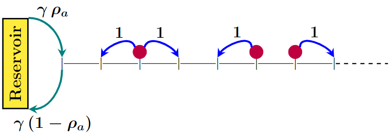
Model and main result: The SSEP on a semi-infinite lattice (see Fig. 1), with sites indexed by , is composed of continuous-time hard-core random walkers hopping to adjacent sites with a unit rate provided the target site is empty. At the boundary site , particles are injected following exclusion with rate and removed at rate , which models [4] coupling with a reservoir of density . For each site at a given time , we assign a binary occupation number that takes values and , depending on whether the site is empty or occupied, respectively. Initially, sites are filled following Bernoulli distribution with a uniform average density .
Our main result concerns the time-integrated current, , which represents the total flux of particles from the reservoir into the system over a time-period . In the hydrodynamic description [58], expressed in terms of coarse-grained density , the flux
| (1) |
measures the net change in the number of particles in the system. In the large limit, its generating function has the asymptotics
| (2a) | |||
| Here, the scaled cumulant generating function (scgf) (subscript ‘si’ denotes semi-infinite) is given by | |||
| (2b) | |||
| where is a function of the parameters defined as [38, 32] | |||
| (2c) | |||
This dependence of scgf on , and through a single function arises from a symmetry of the underlying dynamics of the SSEP [36, 38, 59]. The expression (2b) is consistent with our earlier [54] result in the low-density limit. It is instructive to compare (2b) with the corresponding result for the infinite line [38].
The scgf (2b) encapsulates all cumulants of in the large limit. While the first three cumulants were initially reported in [54], we present here the fourth cumulant for
| (3) |
Similar to the infinite line case [31], the scgf (2b) also admits the Gallavotti-Cohen-type fluctuation symmetry
| (4) |
Remarkably, the expression (2b) admits a Fredholm determinant representation
| (5) |
with the kernel . Analogous Fredholm determinant structure is observed in related contexts for the current distribution in the TASEP [60] and the ASEP [61, 62]. This representation underscores a connection between TASEP and random matrix theory, as emphasized by Johansson [60]. However, a similar relationship for the SSEP is not apparent. Interestingly, an alternative representation of (2b),
| (6) |
bears a striking resemblance 111This perplexing similarity was brought to our attention by Gunter M. Schütz. to the scgf for the number of surviving particles in an assembly of annihilating random walkers (see eq. (9.106) in [16]).
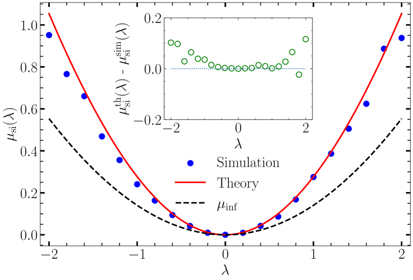
Numerical verification: For confirming our result (2b) based on the hydrodynamic description of SSEP, we have independently generated the scgf using numerical simulation based on a continuous-time cloning algorithm [58, 18, 19] with clones and measured over duration . The simulation result, plotted in Fig. 2, shows a good agreement with our theoretical result (2b) for a reasonably large value of . Deviations emerging at larger values of are a consequence of finite-size effects [58].
LDF: The scaling in (2a) corresponds to a large deviation asymptotics of the probability
| (7) |
where is the ldf, related to (reference to is ignored) by a Legendre-Fenchel transformation [12] . Using the transformation, it is immediate that (4) reflects the symmetry
| (8) |
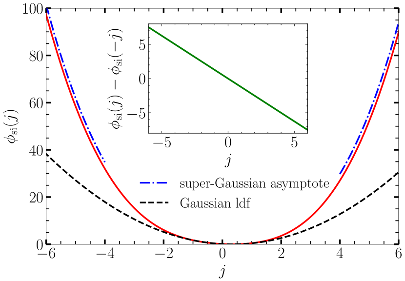
Similarly, the asymptotics of (2b) for large positive correspond [38] to the asymptotics of the ldf
| (9) |
for large positive . A similar analysis for large negative gives asymptotics (9) with and . Notably, for the non-equilibrium condition , the ldf is skewed.
The symmetry relation (8) and the asymptotics (9) are confirmed in the plot of the ldf in Fig. 3, generated by numerically evaluating the Legendre-Fenchel transformation of the scgf (2b).
Derivation: In the following, we outline our derivation of (2b) within the fluctuating hydrodynamics framework of MFT. The crucial idea behind MFT is to recognize the relevant hydrodynamic modes for a coarse-grained description of the dynamics and characterize the probability of their evolution in terms of an Action, which is analogous to the Martin-Siggia-Rose-Janssen-De Dominicis (MSRJD) Action [64, 65, 66, 67] of the associated fluctuating hydrodynamics equation. For SSEP, the relevant hydrodynamic mode is the locally conserved density evolving by [54, 58]
| (10) |
where , and is a delta-correlated Gaussian white noise with unit covariance. Corresponding MSRJD-Action on the semi-infinite line is [54, 58]
| (11) |
where is the response field and incorporates contributions from fluctuations in the initial state [31, 54]. Within this description, the generating function with and in (1).
For large , the path-integral is dominated by a saddle point, leading to (2a) with
| (12) |
(reference to is ignored) where is the least-Action path for . This way, the problem reduces [31, 54] to solving the corresponding Euler-Lagrange equations
| (13a) | ||||
| (13b) | ||||
in the semi-infinite domain , with the temporal boundary conditions
| (14) |
where the integral in is the contribution [31] from for the initial state of the SSEP with Bernoulli measure. Additional spatial boundary conditions,
| (15) |
This variational problem is reminiscent of the corresponding problem on the infinite line [31] for a Bernoulli-measured initial state with an average density for and for . The only differences between the two problems are the domain and the boundary conditions. The infinite line problem was formulated in [31] within MFT, which was recently solved in [39] by identifying an ingenious mapping to the classical integrable system and employing the inverse scattering method. Despite having small differences, the semi-infinite case poses a new nontrivial problem [68], which is incredibly difficult to solve.
A remarkable simplification arises for the special choice of initial density pair for the semi-infinite line problem. For this choice of densities, there are no fluctuations in the initial state, which amounts to setting in (11) with the condition
| (16) |
The Euler-Lagrange equations for the corresponding variational problem (12) remains the same as in (13). The only difference comes in the initial condition in (14), which is now replaced by (16). This initial condition corresponds to the quenched averaging [31, 41].
We now show that this quenched semi-infinite line problem has a direct mapping to the quenched infinite line problem with and fugacity . For the latter problem, the Euler-Lagrange equation is the same [31] as in (13), but now on the entire real line with the temporal boundary conditions
| (17) |
(subscript ‘inf’ denotes infinite). It is trivial to check that the solution admits the symmetry
| (18a) | ||||
| (18b) | ||||
which fixes the value of the fields at the origin
| (19) |
at all times . This conclusion is an essential part of our observation, as now, the solution on positive line satisfies the boundary conditions (15, 16) of the semi-infinite line problem with . For a similar correspondence of the response field, we define
| (20) |
which too now replicates the boundary conditions and of the semi-infinite line problem with . The fields also satisfy the same Euler-Lagrange equations (13).
Consequently, the least-Action path for the semi-infinite line problem with and fugacity is related to the corresponding path for the infinite line problem with and fugacity by
| (21) |
for at all times. This correspondence relates the least-Action of the two problems resulting [58] in our crucial observation:
| (22) |
where the pre-factor comes from the half-domain of integration of in (11). The latter scgf is known from the seminal work [38] of Derrida and Gerschenfeld, which culminates in
| (23) |
The result (23) is for the specific initial density pair . For extending the result for other densities, we invoke a well-known rotational symmetry [31, 59, 58] of the least-Action (12). Essentially, the least-Action paths for two sets of parameters and are related under a canonical transformation [31, 59, 58]. The symmetry results [38, 59, 58] in a dependence of the scgf on through a single parameter
| (24) |
where is defined in (2c). This dependence enables us [58] to deduce the function from the result (23), leading to the expression (2b).
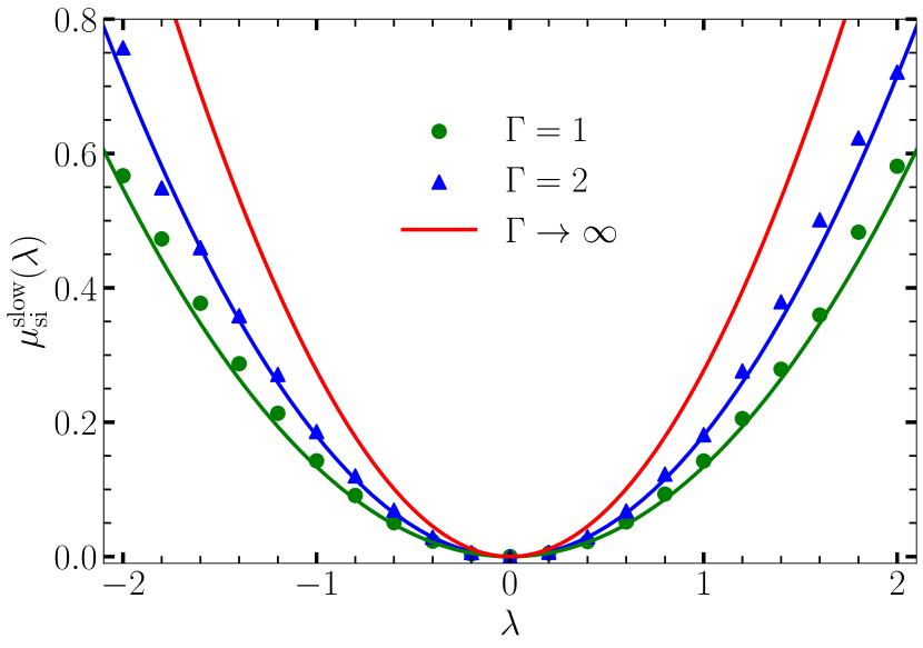
Slow bond: Recent interests [69, 70, 71, 72, 73, 35, 41, 54] in studying the effects of the coupling strength with reservoir can also be addressed in the semi-infinite line problem. The result (2b) is independent [54] of the coupling strength (see Fig. 1) as long as it is larger than . This is seen from the corresponding result for slow coupling , where the boundary-fluctuations are significant, modifying the scgf (2b) to
| (25) |
The expression (25) is obtained following an additivity argument [35], where contributions in (25) are separately from the single bond joining the reservoir and the system, and the system itself, optimised over the density at their common site [58]. This construction is very similar to the discussion in [35] for a related context, except for a crucial distinction that unlike the latter example, there is no quasi-stationarity for the semi-infinite problem. Nevertheless, the additivity conjecture gives the correct result (25), as verified in Fig. 4.
A similar additivity argument helps to solve the problem of current fluctuation across a single slow bond on the infinite lattice [74, 25, *2016_Franco_Phase, 75]. For the hopping rate across the slow bond, and unity for rest of the lattice, the generating function of current , for large , with the scgf
| (26) |
where . In the limit, the celebrated infinite line result [38, 39] is recovered [58] from (26).
Other applications: Several other interesting conclusions can be drawn from our result. A known symmetry [31] of the MFT-Action extends our exact results to models [76, 77, 78] with a quadratic mobility , where and are arbitrary constants, culminating in .
Our semi-infinite line result provides immediate solutions for two closely related problems. The first problem [24] concerns an infinite line SSEP with fast injection at a single site, a scenario which gained prominence in related contexts [79, 80, 81]. At long-times , the net injection of particles on an empty lattice follows the asymptotics with (2b), which results from the statistical independence of the two halves due to fast injection. The second problem concerns the survival probability of the particle (tracer) up to time in a fully packed SSEP on in the presence of an absorbing site at the origin. The asymptotics (7) and the relation with the cumulative probability of integrated current result in a stretched exponential decay for at long-times , with .
Similar stretched exponential decays were noted in kinetically constrained models [82, 23, 83, 84], such as the energy-conserving spin-flip dynamics [23], where spin auto-correlation decays as , with remaining undetermined. For the spin-model, it was realized [84] that the domain-wall dynamics is equivalent to the infinite-line SSEP at a uniform density . This correspondence relates 222This work was initiated from a seminar by Mustansir Barma, who encouraged us to solve the problem. the spin-auto-correlation to the generating function of current in SSEP leading [58] to an exact result , where is the scgf of the infinite line problem [38]. Similar correspondence holds in the presence of slow bond in the spin-flip dynamics, relating to (26).
Conclusions: There remain several related open problems of immediate interest. Most prominent among them is the scgf for fixed (quenched) initial states at arbitrary densities. The only available non-trivial result [31] is for the infinite line SSEP at half-filling, obtained by establishing a relation with the fluctuating (annealed) initial state. A similar mapping for the semi-infinite line yields the quenched scgf
| (27) |
Another pressing open question is the least-Action path at arbitrary densities for the semi-infinite line. In broader contexts, an extension of the problem in higher dimensions would be interesting, where only limited results are available [86]. From a practical point of view, the emergence of the infinite line SSEP in quantum circuits [8] is exciting, and a semi-infinite analog would be worth exploring. Along similar lines, extensions of our results for quantum analogues of the SSEP [87, 88] or for integrable models using generalized hydrodynamics [89, 90] would be timely.
Acknowledgements.
We acknowledge the financial support of the Department of Atomic Energy, Government of India, under Project Identification No. RTI 4002. TS thanks Bernard Derrida for insightful discussions on the problem. The importance of semi-infinite line SSEP and the additivity ansatz for slow bond originated from those discussions. TS also thanks Mustansir Barma for introducing him to the works on stretched exponential decays, particularly the open problem in [23].References
- Prähofer and Spohn [2002] M. Prähofer and H. Spohn, Current fluctuations for the totally asymmetric simple exclusion process, in In and Out of Equilibrium: Probability with a Physics Flavor, Vol. 51, edited by V. Sidoravicius (Birkhäuser Boston, 2002) p. 185–204.
- Bertini et al. [2005] L. Bertini, A. De Sole, D. Gabrielli, G. Jona-Lasinio, and C. Landim, Current fluctuations in stochastic lattice gases, Phys. Rev. Lett. 94, 030601 (2005).
- Bertini et al. [2006] L. Bertini, A. De Sole, D. Gabrielli, G. Jona-Lasinio, and C. Landim, Non equilibrium current fluctuations in stochastic lattice gases, J. Stat. Phys. 123, 237–276 (2006).
- Derrida [2007] B. Derrida, Non-equilibrium steady states: Fluctuations and large deviations of the density and of the current, J. Stat. Mech. 2007, P07023 (2007).
- Lazarescu [2015] A. Lazarescu, The physicist’s companion to current fluctuations: One-dimensional bulk-driven lattice gases, J. Phys. A: Math. Theor. 48, 503001 (2015).
- Banerjee et al. [2020] T. Banerjee, S. N. Majumdar, A. Rosso, and G. Schehr, Current fluctuations in noninteracting run-and-tumble particles in one dimension, Phys. Rev. E 101, 052101 (2020).
- Lee et al. [1995] H. Lee, L. S. Levitov, and A. Y. Yakovets, Universal statistics of transport in disordered conductors, Phys. Rev. B 51, 4079 (1995).
- McCulloch et al. [2023] E. McCulloch, J. De Nardis, S. Gopalakrishnan, and R. Vasseur, Full counting statistics of charge in chaotic many-body quantum systems, Phys. Rev. Lett. 131, 210402 (2023).
- Bodineau and Derrida [2005] T. Bodineau and B. Derrida, Distribution of current in nonequilibrium diffusive systems and phase transitions, Phys. Rev. E 72, 066110 (2005).
- Bodineau et al. [2008] T. Bodineau, B. Derrida, V. Lecomte, and F. van Wijland, Long range correlations and phase transitions in non-equilibrium diffusive systems, J. Stat. Phys. 133, 1013–1031 (2008).
- Jona-Lasinio [2010] G. Jona-Lasinio, From fluctuations in hydrodynamics to nonequilibrium thermodynamics, Prog. Theor. Phys. Supp. 184, 262–275 (2010).
- Touchette [2009] H. Touchette, The large deviation approach to statistical mechanics, Phys. Rep. 478, 1–69 (2009).
- Bertini et al. [2009] L. Bertini, A. De Sole, D. Gabrielli, G. Jona-Lasinio, and C. Landim, Towards a nonequilibrium thermodynamics: A self-contained macroscopic description of driven diffusive systems, J. Stat. Phys. 135, 857–872 (2009).
- Hurtado et al. [2011] P. I. Hurtado, C. Pérez-Espigares, J. J. del Pozo, and P. L. Garrido, Symmetries in fluctuations far from equilibrium, PNAS 108, 7704–7709 (2011).
- Baek et al. [2018] Y. Baek, Y. Kafri, and V. Lecomte, Dynamical phase transitions in the current distribution of driven diffusive channels, J. Phys. A: Math. Theor. 51, 105001 (2018).
- Schütz [2001] G. M. Schütz, Exactly solvable models for many-body systems far from equilibrium, in Phase Transitions and Critical Phenomena, Vol. 19, edited by C. Domb and J. L. Lebowitz (Academic Press, 2001) p. 1–251.
- Mallick [2015] K. Mallick, The exclusion process: A paradigm for non-equilibrium behaviour, Physica A 418, 17–48 (2015).
- Giardinà et al. [2006] C. Giardinà, J. Kurchan, and L. Peliti, Direct evaluation of large-deviation functions, Phys. Rev. Lett. 96, 120603 (2006).
- Lecomte and Tailleur [2007] V. Lecomte and J. Tailleur, A numerical approach to large deviations in continuous time, J. Stat. Mech. 2007, P03004 (2007).
- Giardinà et al. [2011] C. Giardinà, J. Kurchan, V. Lecomte, and J. Tailleur, Simulating rare events in dynamical processes, J. Stat. Phys. 145, 787–811 (2011).
- Pérez-Espigares and Hurtado [2019] C. Pérez-Espigares and P. I. Hurtado, Sampling rare events across dynamical phase transitions, Chaos 29, 083106 (2019).
- Hartmann [2015] A. K. Hartmann, Big Practical Guide to Computer Simulations, 2nd ed. (World Scientific, 2015).
- Spohn [1989] H. Spohn, Stretched exponential decay in a kinetic Ising model with dynamical constraint, Commun. Math. Phys. 125, 3–12 (1989).
- Krapivsky [2012] P. L. Krapivsky, Symmetric exclusion process with a localized source, Phys. Rev. E 86, 041103 (2012).
- Franco et al. [2013a] T. Franco, P. Gonçalves, and A. Neumann, Phase transition in equilibrium fluctuations of symmetric slowed exclusion, Stoch. Process. Their Appl. 123, 4156 (2013a).
- Franco et al. [2016] T. Franco, P. Gonçalves, and A. Neumann, Corrigendum to “Phase transition in equilibrium fluctuations of symmetric slowed exclusion” [Stochastic Process. Appl. 123(12) (2013) 4156–4185], Stoch. Process. Their Appl. 126, 3235 (2016).
- Spohn [1991] H. Spohn, Large Scale Dynamics of Interacting Particles (Springer Berlin, Heidelberg, 1991).
- Kipnis and Landim [1999] C. Kipnis and C. Landim, Scaling Limits of Interacting Particle Systems (Springer Berlin, Heidelberg, 1999).
- Liggett [1999] T. M. Liggett, Stochastic Interacting Systems: Contact, Voter and Exclusion Processes (Springer Berlin, Heidelberg, 1999).
- Chou et al. [2011] T. Chou, K. Mallick, and R. K. P. Zia, Non-equilibrium statistical mechanics: from a paradigmatic model to biological transport, Rep. Prog. Phys. 74, 116601 (2011).
- Derrida and Gerschenfeld [2009a] B. Derrida and A. Gerschenfeld, Current fluctuations in one dimensional diffusive systems with a step initial density profile, J. Stat. Phys. 137, 978–1000 (2009a).
- Krapivsky and Meerson [2012] P. L. Krapivsky and B. Meerson, Fluctuations of current in nonstationary diffusive lattice gases, Phys. Rev. E 86, 031106 (2012).
- Bodineau and Derrida [2004] T. Bodineau and B. Derrida, Current fluctuations in nonequilibrium diffusive systems: An additivity principle, Phys. Rev. Lett. 92, 180601 (2004).
- Bodineau and Derrida [2007] T. Bodineau and B. Derrida, Cumulants and large deviations of the current through non-equilibrium steady states, C. R. Physique 8, 540–555 (2007).
- Derrida et al. [2021] B. Derrida, O. Hirschberg, and T. Sadhu, Large deviations in the symmetric simple exclusion process with slow boundaries, J. Stat. Phys. 182, 15 (2021).
- Derrida et al. [2004] B. Derrida, B. Douçot, and P. E. Roche, Current fluctuations in the one-dimensional symmetric exclusion process with open boundaries, J. Stat. Phys. 115, 717–748 (2004).
- Gorissen et al. [2012] M. Gorissen, A. Lazarescu, K. Mallick, and C. Vanderzande, Exact current statistics of the asymmetric simple exclusion process with open boundaries, Phys. Rev. Lett. 109, 170601 (2012).
- Derrida and Gerschenfeld [2009b] B. Derrida and A. Gerschenfeld, Current fluctuations of the one dimensional symmetric simple exclusion process with step initial condition, J. Stat. Phys. 136, 1–15 (2009b).
- Mallick et al. [2022] K. Mallick, H. Moriya, and T. Sasamoto, Exact solution of the macroscopic fluctuation theory for the symmetric exclusion process, Phys. Rev. Lett. 129, 040601 (2022).
- Mallick et al. [2024] K. Mallick, H. Moriya, and T. Sasamoto, Exact solutions to macroscopic fluctuation theory through classical integrable systems (2024), arXiv:2404.16434 .
- Saha and Sadhu [2023a] S. Saha and T. Sadhu, Large deviations in the symmetric simple exclusion process with slow boundaries: A hydrodynamic perspective (2023a), arXiv:2310.11350v2 .
- Bertini et al. [2015] L. Bertini, A. De Sole, D. Gabrielli, G. Jona-Lasinio, and C. Landim, Macroscopic fluctuation theory, Rev. Mod. Phys. 87, 593 (2015).
- Jona-Lasinio [2023] G. Jona-Lasinio, Review article: Large fluctuations in non-equilibrium physics, Nonlin. Processes Geophys. 30, 253–262 (2023).
- Bertini et al. [2001] L. Bertini, A. De Sole, D. Gabrielli, G. Jona-Lasinio, and C. Landim, Fluctuations in stationary nonequilibrium states of irreversible processes, Phys. Rev. Lett. 87, 040601 (2001).
- Bertini et al. [2002] L. Bertini, A. De Sole, D. Gabrielli, G. Jona-Lasinio, and C. Landim, Macroscopic fluctuation theory for stationary non-equilibrium states, J. Stat. Phys. 107, 635–675 (2002).
- Tailleur et al. [2007] J. Tailleur, J. Kurchan, and V. Lecomte, Mapping nonequilibrium onto equilibrium: The macroscopic fluctuations of simple transport models, Phys. Rev. Lett. 99, 150602 (2007).
- Tailleur et al. [2008] J. Tailleur, J. Kurchan, and V. Lecomte, Mapping out-of-equilibrium into equilibrium in one-dimensional transport models, J. Phys. A: Math. Theor. 41, 505001 (2008).
- Bettelheim et al. [2022a] E. Bettelheim, N. R. Smith, and B. Meerson, Inverse scattering method solves the problem of full statistics of nonstationary heat transfer in the Kipnis-Marchioro-Presutti model, Phys. Rev. Lett. 128, 130602 (2022a).
- Bettelheim et al. [2022b] E. Bettelheim, N. R. Smith, and B. Meerson, Full statistics of nonstationary heat transfer in the Kipnis–Marchioro–Presutti model, J. Stat. Mech. 2022, 093103 (2022b).
- Agranov et al. [2023] T. Agranov, S. Ro, Y. Kafri, and V. Lecomte, Macroscopic fluctuation theory and current fluctuations in active lattice gases, SciPost Phys. 14, 045 (2023).
- Bettelheim and Meerson [2024] E. Bettelheim and B. Meerson, Complete integrability of the problem of full statistics of nonstationary mass transfer in the simple inclusion process (2024), arXiv:2403.19536v2 .
- Liggett [1975] T. M. Liggett, Ergodic theorems for the asymmetric simple exclusion process, Trans. Am. Math. Soc. 213, 237–261 (1975).
- Grosskinsky [2004] S. Grosskinsky, Phase transitions in nonequilibrium stochastic particle systems with local conservation laws, Ph.D. thesis, Technical University of Munich (2004).
- Saha and Sadhu [2023b] S. Saha and T. Sadhu, Current fluctuations in a semi-infinite line, J. Stat. Mech. 2023, 073207 (2023b).
- Williams and Sasamoto [2012] L. Williams and T. Sasamoto, Combinatorics of the asymmetric exclusion process on a semi-infinite lattice (2012), arXiv:1204.1114 .
- Tracy and Widom [2013] C. A. Tracy and H. Widom, The asymmetric simple exclusion process with an open boundary, J. Math. Phys. 54, 103301 (2013).
- Duhart et al. [2018] H. G. Duhart, P. Mörters, and J. Zimmer, The semi-infinite asymmetric exclusion process: Large deviations via matrix products, Potential Anal. 48, 301–323 (2018).
- [58] See Supplementary Material for details.
- Lecomte et al. [2010] V. Lecomte, A. Imparato, and F. van Wijland, Current fluctuations in systems with diffusive dynamics, in and out of equilibrium, Prog. Theor. Phys. Suppl. 184, 276–289 (2010).
- Johansson [2000] K. Johansson, Shape fluctuations and random matrices, Comm. Math. Phys. 209, 437–476 (2000).
- Tracy and Widom [2008] C. A. Tracy and H. Widom, A fredholm determinant representation in ASEP, J. Stat. Phys. 132, 291–300 (2008).
- Tracy and Widom [2009] C. A. Tracy and H. Widom, Total current fluctuations in the asymmetric simple exclusion process, J. Math. Phys. 50, 095204 (2009).
- Note [1] This perplexing similarity was brought to our attention by Gunter M. Schütz.
- Martin et al. [1973] P. C. Martin, E. D. Siggia, and H. A. Rose, Statistical dynamics of classical systems, Phys. Rev. A 8, 423 (1973).
- Janssen [1976] H. K. Janssen, On a Lagrangean for classical field dynamics and renormalization group calculations of dynamical critical properties, Z. Physik B 23, 377–380 (1976).
- De Dominicis [1978] C. De Dominicis, Dynamics as a substitute for replicas in systems with quenched random impurities, Phys. Rev. B 18, 4913 (1978).
- De Dominicis and Peliti [1978] C. De Dominicis and L. Peliti, Field-theory renormalization and critical dynamics above : Helium, antiferromagnets, and liquid-gas systems, Phys. Rev. B 18, 353 (1978).
- Ablowitz and Segur [1975] M. J. Ablowitz and H. Segur, The inverse scattering transform: Semi-infinite interval, J. Math. Phys. 16, 1054–1056 (1975).
- Baldasso et al. [2017] R. Baldasso, O. Menezes, A. Neumann, and R. R. Souza, Exclusion process with slow boundary, J. Stat. Phys. 167, 1112–1142 (2017).
- Franco et al. [2019] T. Franco, P. Gonçalves, and A. Neumann, Non-equilibrium and stationary fluctuations of a slowed boundary symmetric exclusion, Stoch. Process. Their Appl. 129, 1413–1442 (2019).
- Gonçalves et al. [2020] P. Gonçalves, M. Jara, O. Menezes, and A. Neumann, Non-equilibrium and stationary fluctuations for the SSEP with slow boundary, Stoch. Process. Their Appl. 130, 4326–4357 (2020).
- Erignoux et al. [2020a] C. Erignoux, P. Gonçalves, and G. Nahum, Hydrodynamics for SSEP with non-reversible slow boundary dynamics: Part I, the critical regime and beyond, J. Stat. Phys. 181, 1433–1469 (2020a).
- Erignoux et al. [2020b] C. Erignoux, P. Gonçalves, and G. Nahum, Hydrodynamics for SSEP with non-reversible slow boundary dynamics: Part II, below the critical regime, ALEA, Lat. Am. J. Probab. Math. Stat. 17, 791–823 (2020b).
- Franco et al. [2013b] T. Franco, P. Gonçalves, and A. Neumann, Hydrodynamical behavior of symmetric exclusion with slow bonds, Ann. Inst. H. Poincaré Probab. Statist. 49, 402–427 (2013b).
- Erhard et al. [2020] D. Erhard, T. Franco, P. Gonçalves, A. Neumann, and M. Tavares, Non-equilibrium fluctuations for the SSEP with a slow bond, Ann. Inst. H. Poincaré Probab. Statist. 56, 1099–1128 (2020).
- Kipnis et al. [1982] C. Kipnis, C. Marchioro, and E. Presutti, Heat flow in an exactly solvable model, J. Stat. Phys. 27, 65–74 (1982).
- Schütz and Sandow [1994] G. Schütz and S. Sandow, Non-Abelian symmetries of stochastic processes: Derivation of correlation functions for random-vertex models and disordered-interacting-particle systems, Phys. Rev. E 49, 2726 (1994).
- Giardinà et al. [2007] C. Giardinà, J. Kurchan, and F. Redig, Duality and exact correlations for a model of heat conduction, J. Math. Phys. 48, 033301 (2007).
- Krapivsky and Stefanovic [2014] P. L. Krapivsky and D. Stefanovic, Lattice gases with a point source, J. Stat. Mech. 2014, P09003 (2014).
- Krapivsky et al. [2019] P. L. Krapivsky, K. Mallick, and D. Sels, Free fermions with a localized source, J. Stat. Mech. 2019, 113108 (2019).
- Krapivsky et al. [2020] P. L. Krapivsky, K. Mallick, and D. Sels, Free bosons with a localized source, J. Stat. Mech. 2020, 063101 (2020).
- Skinner [1983] J. L. Skinner, Kinetic Ising model for polymer dynamics: Applications to dielectric relaxation and dynamic depolarized light scattering, J. Chem. Phys. 79, 1955–1964 (1983).
- Gupta et al. [2020] V. Gupta, S. K. Nandi, and M. Barma, Size-stretched exponential relaxation in a model with arrested states, Phys. Rev. E 102, 022103 (2020).
- Mukherjee et al. [2024] S. Mukherjee, P. Pareek, M. Barma, and S. K. Nandi, Stretched exponential to power-law: crossover of relaxation in a kinetically constrained model, J. Stat. Mech. 2024, 023205 (2024).
- Note [2] This work was initiated from a seminar by Mustansir Barma, who encouraged us to solve the problem.
- Akkermans et al. [2013] E. Akkermans, T. Bodineau, B. Derrida, and O. Shpielberg, Universal current fluctuations in the symmetric exclusion process and other diffusive systems, EPL 103, 20001 (2013).
- Bernard and Jin [2019] D. Bernard and T. Jin, Open quantum symmetric simple exclusion process, Phys. Rev. Lett. 123, 080601 (2019).
- Bernard [2021] D. Bernard, Can the macroscopic fluctuation theory be quantized?, J. Phys. A: Math. Theor. 54, 433001 (2021).
- Doyon [2020] B. Doyon, Lecture notes on generalised hydrodynamics, SciPost Phys. Lect. Notes , 18 (2020).
- Bastianello et al. [2022] A. Bastianello, B. Bertini, B. Doyon, and R. Vasseur, Introduction to the special issue on emergent hydrodynamics in integrable many-body systems, J. Stat. Mech. 2022, 014001 (2022).