Electronic Coherences in Molecules: The Projected Nuclear Quantum Momentum as a Hidden Agent

Abstract

Electronic coherences are key to understanding and controlling photo-induced molecular transformations. We identify a crucial quantum-mechanical feature of electron-nuclear correlation, the projected nuclear quantum momenta, essential to capture the correct coherence behavior. In simulations, we show that, unlike traditional trajectory-based schemes, exact-factorization-based methods approximate these correlation terms, and correctly capture electronic coherences in a range of situations, including their spatial dependence, an important aspect that influences subsequent electron dynamics and that is becoming accessible in more experiments.

In photo-induced processes, quantum electronic coherences are key factors influencing many molecular processes. They can serve as control knobs in chemical transformations  Kaufman et al. (2023); Garg et al. (2022); Mogol et al. (2023); Despré et al. (2018); Dey et al. (2022); Vacher et al. (2017) and possibly impact photosynthetic energy flow in biomolecules Duan et al. (2017); Maiuri et al. (2018), as well as quantum information science processes Wasielewski et al. (2020). Aside from the practical interest in creating desired products, studying the generation and evolution of these coherences, including both decay and revival, reveals fundamental properties of how correlations between electrons as well as their interplay with nuclei affect dynamics. Experiments can now track how coherences evolve in time with spatial resolution as well Cavaletto et al. (2021); Garg et al. (2022); Mogol et al. (2023).

While coherence is generally a representation-independent concept, we tend to consider them in the Born-Oppenheimer (BO) picture, for the physical reason that away from regions of strong non-adiabatic coupling (NAC), components of the nuclear wavefunction on different BO surfaces evolve independently. We define the spatially-resolved electronic coherence as

$$\Gamma_{jk}({\underline{\underline{\bf R}}},t)=\chi_{j}^{*}({\underline{\underline{\bf R}}},t)\chi_{k}({\underline{\underline{\bf R}}},t)$$ (1)

for $j\neq k$ (and populations $j=k$), where the $\chi_{j}({\underline{\underline{\bf R}}},t)$ are projected nuclear wavefunctions defined via expanding the full molecular wavefunction in the BO basis: $\Psi({\underline{\underline{\bf R}}},{\underline{\underline{\bf r}}},t)=\sum_{j}\chi_{j}({\underline{\underline{\bf R}}},t)\Phi_{{\underline{\underline{\bf R}}},j}({\underline{\underline{\bf r}}})$, with $\Phi_{{\underline{\underline{\bf R}}},j}$ eigenstates of the BO Hamiltonian $H_{\rm BO}|\Phi_{{\underline{\underline{\bf R}}},j}\rangle=E_{j}^{\rm BO}|\Phi_{{\underline{\underline{\bf R}}},j}\rangle$ and with variables ${\underline{\underline{\bf r}}}$, ${\underline{\underline{\bf R}}}$ denoting all electronic and nuclear coordinates, respectively. While recent advances in experimental techniques allow to measure the electronic coherences with angstrom spatial resolution, most experiments instead measure the spatially-integrated coherence, $\Gamma_{jk}(t)=\int d{\underline{\underline{\bf R}}}\Gamma_{jk}({\underline{\underline{\bf R}}},t)$, often referred to as coherence tout court. The electronic coherence measures the overlap of the projected wavefunctions, and when different surfaces have different slopes, in regions of negligible NAC, these wavefunctions evolve away from each other leading to decaying coherence, a phenomenon often referred to as decoherence. However, open questions remain in the nature of the electron-nuclear correlation in influencing coherences, decoherences, and recoherences (i.e. revivals after decoherence): How significant is the spatial-structure in Eq. 1, an inherent signature of this correlation, especially if an experiment cannot resolve it? Is a purely classical point-like description of the nuclear motion enough or are quantum properties arising from the width, internal structure, and phases of the nuclear wavepackets key?

Consistent theoretical simulations of coherence and decoherence in photo-excited molecules have proven to be challenging, requiring an adequate description of both electron-electron interaction as well as electron-nuclear correlation. The molecules of interest are typically large enough that mixed quantum-classical (MQC) approximations are made which run an ensemble of classical nuclear trajectories each carrying a set of quantum electronic coefficients. The commonly-used methods, Ehrenfest and surface-hopping Tully (1990, 1998) are both fundamentally unable to correctly capture coherence: while the electronic coefficients in Ehrenfest always remain coherent, those in surface-hopping are inconsistent with the trajectory-evolution and utilize a largely ad hoc decoherence procedure Granucci and Persico (2007); Wang et al. (2016); Crespo-Otero and Barbatti (2018); Subotnik et al. (2016). Ref. Esch and Levine (2020) pointed out that the commonly-used decoherence corrections are fundamentally flawed in that they act in a state-wise manner while coherence is a state pair-wise property.

We show that even when only the spatially-integrated coherence is measured, the underlying spatial-dependence strongly influences the time-dependence, and that the projected nuclear quantum momenta, $\nabla_{\nu}|\chi_{j}|/|\chi_{j}|$, are key to capturing the correct behavior. Thus electron-nuclear correlation terms that go beyond a classical picture of the nuclei are essential. In simulations, this means that even in cases where traditional MQC methods yield the correct coherence over the duration of one interaction event, their wrong spatially-resolved coherence leads to poor behavior at longer times. Instead, MQC methods based on the exact factorization (EF) approach Min et al. (2015); Agostini et al. (2016); Ha et al. (2018); Villaseco Arribas and Maitra (2023); Dupuy et al. (2024) better approximate the spatial structure, and give greatly improved predictions, distinguishing between coherence of wavefunctions on parallel surfaces (unlike ad hoc decoherence-corrected methods) and gradual decoherence of non-parallel ones (unlike Ehrenfest). While the existing EF-based approximations contain a crucial dependence on the overall nuclear quantum momentum, we identify their neglect of the individually projected quantities as the culprit for not accurately capturing recoherence events in regions of negligible NAC.

Coherences evolve due to population transitions from NACs ($\langle\Phi_{{\underline{\underline{\bf R}}},j}|\nabla_{\nu}\Phi_{{\underline{\underline{\bf R}}},k}\rangle$ and $\langle\Phi_{{\underline{\underline{\bf R}}},j}|\nabla_{\nu}^{2}\Phi_{{\underline{\underline{\bf R}}},k}\rangle$), but also away from those regions when more than one BO surface is populated. To avoid conflating effects from NACs, we begin by considering the exact equation of motion for the spatially-resolved coherence in a situation where all NACs are zero:

$$i\partial_{t}\Gamma_{jk}({\underline{\underline{\bf R}}},t) = \Delta E_{kj}({\underline{\underline{\bf R}}})\Gamma_{jk}({\underline{\underline{\bf R}}},t)+\sum_{\nu}\frac{1}{2M_{\nu}}\bigg{(}\chi_{k}({\underline{\underline{\bf R}}},t)$$ (2)

$$\nabla_{\nu}^{2}\chi_{j}^{*}({\underline{\underline{\bf R}}},t)-\chi_{j}^{*}({\underline{\underline{\bf R}}},t)\nabla_{\nu}^{2}\chi_{k}({\underline{\underline{\bf R}}},t)\bigg{)}$$

where $\Delta E_{kj}({\underline{\underline{\bf R}}})=E^{\rm BO}_{k}({\underline{\underline{\bf R}}})-E^{\rm BO}_{j}({\underline{\underline{\bf R}}})$ and the sum over $\nu$ is a sum over all nuclei. Atomic units ($\hbar=m_{e}=e^{2}=1$) are used throughout this article. The first term on the right of Eq. 2 can be absorbed in a phase, such that the magnitude of the spatially-resolved coherence depends only the curvatures of the BO projected wavefunctions and not explicitly on the shape of the BO surfaces. Instead, when integrated over space, the explicit dependence on these curvatures vanishes, and we find

$$i\partial_{t}\Gamma_{jk}(t)=\int\Delta E_{kj}({\underline{\underline{\bf R}}})\Gamma_{kj}({\underline{\underline{\bf R}}},t)d{\underline{\underline{\bf R}}}\,,$$ (3)

that is, the spatially-integrated coherence explicitly depends only on the relative difference in shape of the BO surfaces. We make two key observations from Eqs. 2– 3: First, without correct spatial dependence of the coherence (a dependence that inherently signifies electron-nuclear correlation), the time-evolution of the spatially-integrated coherence or populations will be wrong. Second, for parallel surfaces the spatially-integrated coherence evolve by merely a phase $\Gamma_{jk}(t)=e^{i(E_{k}-E_{j})t}\Gamma_{jk}(0)$, and while their magnitude is constant in time, there is a spatial structure to these quantities that does evolve in time (last two terms of Eq. (2)).

While nuclear motion influences electronic coherences a deeper understanding of this correlation requires to discern effects arising from classical point-like nuclear motion and quantum effects from nuclear wavepacket delocalization. To address this, we turn to the EF, where the full molecular wavefunction takes the form of a single correlated product, $\Psi({\underline{\underline{\bf r}}},{\underline{\underline{\bf R}}},t)=\chi({\underline{\underline{\bf R}}},t)\Phi_{\underline{\underline{\bf R}}}({\underline{\underline{\bf r}}},t)$ with $\int|\Phi_{\underline{\underline{\bf R}}}({\underline{\underline{\bf r}}},t)|^{2}d{\underline{\underline{\bf r}}}=1\,\forall\,{\underline{\underline{\bf R}}},t$ Hunter (1975a, b, 1980, 1981); Hunter and Tai (1982); Gidopoulos and Gross (2014); Abedi et al. (2010, 2012); Agostini and Gross (2021); Villaseco Arribas et al. (2022). (See also Supplementary Material for brief details from these works). The EF yields the notion of a unique nuclear wavefunction that satisfies a Hamiltonian evolution and whose modulus and phase give the exact nuclear density and nuclear current-density, ${\bf J}_{\nu}({\underline{\underline{\bf R}}},t)$, of the molecular wavefunction Abedi et al. (2010, 2012). This allows a formulation of exact unique trajectory-based equations defining exact unique forces on the nuclear trajectories when they are treated classically Li et al. (2022); Agostini et al. (2014); Abedi et al. (2014), and evolution equations for the populations and coherences, as we will see shortly.

Writing the EF nuclear wavefunction in terms of an amplitude and phase, $\chi({\underline{\underline{\bf R}}},t)=e^{iS({\underline{\underline{\bf R}}},t)}|\chi({\underline{\underline{\bf R}}},t)|$, and likewise for the projected BO wavefunctions, $\chi_{k}({\underline{\underline{\bf R}}},t)=|\chi_{k}({\underline{\underline{\bf R}}},t)|e^{iS_{k}({\underline{\underline{\bf R}}},t)}$, we have, in the limit of negligible NAC,

$$\partial_{t}|\Gamma_{jk}({\underline{\underline{\bf R}}},t)|=-|\Gamma_{jk}({\underline{\underline{\bf R}}},t)|\sum_{\nu}\Bigg{\{}\frac{\big{(}\nabla_{\nu}-2\overline{\mathfrak{S}}_{\nu,jk}\big{)}\cdot\mathbb{J}_{\nu}}{|\chi|^{2}}$$

$$+\sum_{n}\frac{|C_{n}|^{2}}{2M_{\nu}}\bigg{[}\overline{\bigg{(}4{\mathbfcal{Q}}_{\nu,jk}-2\nabla_{\nu}\bigg{)}\cdot\big{(}\mathbf{f}_{\nu,n}-\mathbf{f}_{\nu,jk}\big{)}}+4\mathfrak{S}_{\nu,n}\cdot\mathbf{f}_{\nu,n}\bigg{]}\Bigg{\}}$$

(4)

In Eq. 4, all quantities on the right are functions of ${\underline{\underline{\bf R}}}$ and $t$, an overline indicates the average over $j,k$ ($\overline{g}_{jk}=(g_{j}+g_{k})/2$), and we have defined ${\bf f}_{\nu,k}=\nabla_{\nu}(S_{k}-S)$. Further, we defined the nuclear quantum momentum $\mathbf{Q}_{\nu}$ and projected components $\mathbfcal{Q}_{k,\nu}$ for each state $k$ through

$${\bf Q}_{\nu}=-\frac{\nabla_{\nu}|\chi({\underline{\underline{\bf R}}},t)|}{|\chi({\underline{\underline{\bf R}}},t)|}\;{\rm and}\;\mathbfcal{Q}_{k,\nu}({\underline{\underline{\bf R}}},t)=-\frac{\nabla_{\nu}|\chi_{k}({\underline{\underline{\bf R}}},t)|}{|\chi_{k}({\underline{\underline{\bf R}}},t)|}$$ (5)

while $\mathfrak{S}_{\nu,k}$ is the “reduced” contribution

$$\mathfrak{S}_{\nu,k}({\underline{\underline{\bf R}}},t)=-\frac{\nabla_{\nu}|C_{k}({\underline{\underline{\bf R}}},t)|}{|C_{k}({\underline{\underline{\bf R}}},t)|}={\mathbfcal Q}_{\nu,k}-{\bf Q}_{\nu}$$ (6)

with $C_{k}=\chi_{k}/\chi$, which represent coefficients of the conditional electronic wavefunction $\Phi_{\underline{\underline{\bf R}}}({\underline{\underline{\bf r}}},t)$ when expanded in the BO basis, $\Phi_{\underline{\underline{\bf R}}}({\underline{\underline{\bf r}}},t)=\sum_{n}C_{n}({\underline{\underline{\bf R}}},t)\Phi_{{\underline{\underline{\bf R}}},n}({\underline{\underline{\bf r}}})$.

Our third key observation follows from Eq. (4): While the first term on the right represents a convective contribution to the time-derivative (see more shortly), both the projected quantum momentum ${\mathbfcal{Q}}_{\nu,k}$ and the reduced contribution $\mathfrak{S}_{\nu,k}$, play a crucial role in capturing accurate spatially-resolved populations and coherences, when away from NAC regions. The only other term driving (the magnitude of) the coherence or population evolution, $\sum_{n}|C_{n}|^{2}\nabla_{\nu}\cdot({\bf f}_{\nu,k}-{\bf f}_{\nu,n})$, depends on the difference in curvature of the adiabatic phases, which semiclassically relates to the curvatures of the BO surfaces (see more shortly). A fourth key observation is that in regions where the coherence between two states has locally collapsed to zero, only the terms depending on $\mathfrak{S}_{\nu,n}$ survive to drive time-evolution of the spatially-resolved coherences and populations; this is responsible for recoherence effects away from NACs.

Because it is rooted in the EF picture, which enables a unique and unambiguous definition of the total nuclear density and and current-density, we can use Eq. (4) to derive an exact trajectory-based equation for the populations and coherences. We represent the nuclear density as a sum over $\delta$-functions (or very narrow Gaussians) centered at a trajectory position ${\underline{\underline{\bf R}}}^{(I)}(t)$

$$|\chi({\underline{\underline{\bf R}}},t)|^{2}\rightarrow\frac{1}{N_{tr}}\sum_{I}\delta({\underline{\underline{\bf R}}}-{\underline{\underline{\bf R}}}^{(I)}(t))$$ (7)

where ${\underline{\underline{\bf R}}}^{(I)}(t)$ satisfy classical Newton’s equations Min et al. (2015); Agostini et al. (2016) with a generalized Lorentz force dependent on $\Phi_{\underline{\underline{\bf R}}}$ that drives the nuclear motion Agostini et al. (2014); Abedi et al. (2014); Li et al. (2022). The phase $S$ becomes $\nabla_{\nu}S\rightarrow M_{\nu}\dot{{\underline{\underline{\bf R}}}}(t)-{\bf A}$ where ${\bf A}$ is the vector potential in the nuclear Hamiltonian (see Supplemental Material), and the time-derivative along the trajectory given by the convective derivative $d/dt=\partial_{t}+\sum_{\nu}\dot{{\bf R}}^{(I)}_{\nu}\cdot\nabla_{\nu}$. The spatially-resolved and -averaged coherences and populations become trajectory-ensembles:

$$\Gamma_{jk}({\underline{\underline{\bf R}}},t) \rightarrow \frac{1}{N_{tr}}\sum_{I}\delta({\underline{\underline{\bf R}}}-{\underline{\underline{\bf R}}}^{(I)}(t))C_{j}^{(I)*}(t)C_{k}^{(I)}(t)$$

$$\Gamma_{jk}(t) \rightarrow \sum_{I}C_{j}^{(I)*}(t)C_{k}^{(I)}(t)$$ (8)

Then Eq. 4 becomes

$$\frac{d|C_{j}^{*}C_{k}|}{dt}^{(I)}=-\left|C_{j}^{*(I)}C_{k}^{(I)}\right|\,\sum_{\nu,n}\frac{|C_{n}^{(I)}|^{2}}{2M_{\nu}}$$

$$\bigg{[}\overline{\left(4{\mathbfcal{Q}}_{\nu,jk}^{(I)}-2\nabla_{\nu}\right)\cdot\left(\mathbf{f}_{\nu,l}^{(I)}-\mathbf{f}_{\nu,jk}^{(I)}\right)}+4\mathfrak{S}_{\nu,n}^{(I)}\cdot\mathbf{f}_{\nu,n}^{(I)}\bigg{]}$$ (9)

where all are functions of $t$ alone, and we use the short-hand $g^{(I)}=g({\underline{\underline{\bf R}}}^{(I)}(t))$.

Away from any NAC, Eq. 9 gives the exact equation for the magnitude of the electronic populations and coherences that trajectory-based methods should be aiming for. The full equation including the NACs, and phases, is given in the Supplementary Material. The $I$-dependence gives the spatially-resolved character in the trajectory-picture: while the electronic populations and coherences for the case of parallel surfaces $C_{j}^{*(I)}C_{k}^{(I)}(t)$ of individual trajectories ${\underline{\underline{\bf R}}}^{(I)}(t)$ evolve in time, their sum over trajectories should yield remain constant in the limit of a large sampling of the initial distribution, analogous to the discussion below Eq. (3). Time-dependence of the individual $C_{k}^{(I)}(t)$ indicates spatial-dependence in the coefficients, which is crucial in order to get the correct populations and coherences, even when only ensemble-averaged quantities are measurable, as discussed earlier and as we will see explicitly in some examples shortly.

The traditional trajectory-based methods (Ehrenfest, surface-hopping) give strictly zero time-evolution throughout the ensemble in the absence of NACs because they have no such terms, and ad hoc decoherence corrections to surface-hopping cause spurious decays. Our examples will demonstrate this has drastic consequences for intermediate and long-term coherence and population dynamics. The prime importance of the projected quantum momenta in these terms is, on the other hand, partially recognized in the EF-based CTMQC method Min et al. (2015); Agostini et al. (2016), which approximates these terms. Derived from a well-defined series of approximations on the exact electronic and nuclear equations, the resulting CTMQC equations neglect $\mathfrak{S}_{\nu,k}$, effectively approximating $\mathbfcal{Q}_{\nu,k}$ by ${\bf Q}_{\nu}\,\,\,\forall\,k,\nu$. We find (again, for negligible NAC)

$$\left(\frac{d|C_{j}^{*}C_{k}|}{dt}\right)^{(I)}_{\mathrm{exact}}=\left(\frac{d|C_{j}^{*}C_{k}|}{dt}\right)^{(I)}_{\mathrm{CTMQC}}+|C_{j}^{*(I)}C_{k}^{(I)}|$$

$$\sum_{\nu,n}\frac{|C_{n}^{(I)}|^{2}}{2M_{\nu}}\bigg{[}\overline{\big{(}4\mathfrak{S}_{\nu,jk}^{(I)}-2\nabla_{\nu}\big{)}\cdot\big{(}\mathbf{f}_{\nu,n}^{(I)}-\mathbf{f}_{\nu,jk}^{(I)}}\big{)}+4\mathfrak{S}_{\nu,n}^{(I)}\cdot\mathbf{f}_{\nu,n}^{(I)}\bigg{]}$$

(10)

This expression assumes the semiclassical approximation for the gradient of the phase of the electronic coefficients ${\bf f}_{\nu,l}^{(I)}=-\int_{0}^{t}\nabla_{\nu}E_{l}^{(I)}\,dt$, valid away from NACs Agostini et al. (2016). A consequence of CTMQC’s neglect of $\mathfrak{S}$ would be spurious population transfer in regions of zero NAC that is however fixed in implementations by modifying the definition of the quantum momentum to enforce no net transfer in these cases Min et al. (2015); Agostini et al. (2016); Min et al. (2017). However, another consequence, that is not fixed by this redefinition, is CTMQC’s inability to capture recoherence away from NAC regions (see the fourth observation made earlier, and the example shortly).

Our first example is a slight variation on the one-dimensional three-state model of Ref Esch and Levine (2020), which we name EL20-SAC, consisting of two parallel electronic states that eventually reach a single avoided crossing (SAC) Tully (1990), and a third non-parallel state uncoupled to the other two, as shown in the inset of Fig. 1. The Hamiltonian is given in the Supplementary Material. The system is initialized in a $50:25:25$ coherent superposition of three gaussian nuclear wavepackets with center momentum $40$ bohr^-1 and position $-26$ bohr. Despite its simplicity, the model illustrates fundamental aspects of electronic coherences. First, their pair-wise nature Esch and Levine (2020): coherence between the pair of parallel states should be maintained while coherence between non-parallel states should be lost as the distinct forces lead to diverging wavepackets. Second, the need to accurately describe the spatially-resolved coherence, as this is key to correctly capture the dynamics even of spatially-integrated quantities, when entering later into the NAC region.

Figure 1 shows the magnitude of the spatially-integrated electronic coherences between the parallel states (upper panel), non-parallel states (middle panel), and population of the first excited state (lowest panel), obtained from Ehrenfest, CTMQC, surface-hopping with energy-based decoherence correction (SHEDC) Granucci and Persico (2007); Granucci et al. (2010), exact-factorization-based surface-hopping (SHXF) Ha et al. (2018); Lee et al. (2021), and the exact calculations. Simulation details are provided in the Supplemental Material; we use the G-CTMQC code Agostini et al. (Last accessed Oct 2023) for all calculations except the SHXF which is done in PyUnixMD Lee et al. (2021). Consider first the time before the SAC is reached. While Ehrenfest remains coherent, and thus captures the (spatially-integrated) coherence between the parallel surfaces well, it fails to capture the decoherence between the non-parallel surfaces, while the opposite is true of SHEDC in which the parallel coherence erroneously decays and the non-parallel decays much too quickly. In contrast, CTMQC does a good job for both coherences. With the more approximate SHXF, the non-parallel coherence decay time is a little too long, and the parallel coherence shows some deviation from constant. All methods capture the populations well at early times. However, once they reach the SAC, only CTMQC is able to reasonably capture the population and coherence dynamics at the right time, albeit with an overestimation, before settling to about the right values after the non-adiabatic event. SHXF gets the trend in the right direction, but the timing and duration of the event is too long. However the traditional methods are completely wrong: SHEDC shows hardly any transfer and completely wrong coherence behavior, and Ehrenfest’s population goes in the wrong direction.

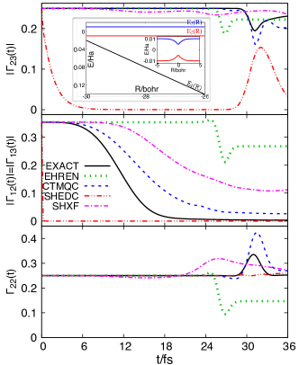
Figure 1: Electronic state populations of the first excited state (lower panel), and magnitude of electronic coherences between non-parallel (medium panel) and parallel states (upper panel) as a function of time for EL20-SAC model whose adiabatic PES is shown in the inset of the top panel. The NAC is only non-zero in the region of the SAC localized at $R=0$.

Why the spatially-integrated electronic quantities are so poor at later times in the traditional methods is revealed by inspecting the spatially-resolved quantities at earlier times, as plotted in Fig. 2. The effect of the projected quantum-momentum terms in the equation of motion creates spatial structure in the coherence (also populations, not shown) that is completely missing in the traditional methods, that nevertheless correctly ensemble-average to zero at times before the SAC is reached. Even if not measured in experiment, the incorrect spatial structure of the coherence in Ehrenfest and SHEDC lead to incorrect ensemble-averaged populations and coherences at later times, as trajectories enter the SAC with wrong coefficients.

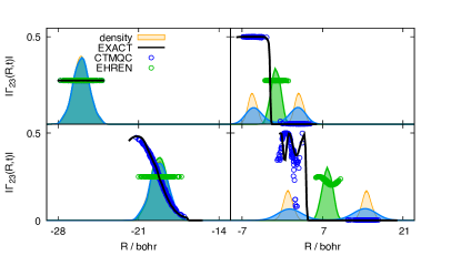
Figure 2: Time snapshots of the exact density, density reconstructed from the distribution of CTMQC and EHREN trajectories and spatially-resolved electronic coherences between the two parallel surfaces with exact, CTMQC , and Ehrenfest.

Our second model, denoted 3HO, consists of three uncoupled harmonic oscillators, two of which are parallel (inset of figure 3); the Hamiltonian is given in the Supplementary Material. The system is initialized in a $50:25:25$ coherent superposition of three gaussian nuclear wavepackets with zero momentum centered at $-4$ bohr. While the wavepackets on the parallel surface maintain constant coherence, they show successive decoherence and recoherence events with the wavepacket on the non-parallel surface. Figure 3 shows, similar to the EL20-SAC model, that while Ehrenfest maintains coherence between parallel and non parallel states, SHEDC shows decoherence for both. SHXF shows similar behavior to SHEDC, and they both suffer from spurious population transfer Villaseco Arribas et al. (2022) as evidenced in the bottom panel. CTMQC on the other hand, shows the correct behavior capturing the first decoherence event while predicting constant spatially-integrated coherences between the parallel surfaces, and correctly constant populations, due its redefinition of the quantum momentum preventing spurious net transfer. However, the recoherence is not well-captured in the EF-based methods. This is because we enter the domain of the fourth observation made earlier where, after the first decoherence, the $\mathfrak{S}_{n}$ are the only terms that can drive coherence change, and CTMQC sets this term to zero. The importance of $\mathfrak{S}$ is evident from the snapshots of the exact $Q$, $\mathcal{Q}_{1}$ and $\mathfrak{S}_{1}$ during the first recoherence event shown in the Supplemental Material (Fig. SI.1), where $\mathfrak{S}$ displays large features that largely cancel those in $Q$, crunching it down to yield a relatively small $\mathcal{Q}_{k}$.

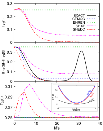
Figure 3: Electronic state populations of the first excited state (lower panel), and magnitude of electronic coherences between non parallel (medium panel) and parallel states (upper panel) as a function of time for 3HO model. The inset shows the adiabatic PES for 3HO model.

In summary, electronic coherences are significantly influenced by beyond-classical electron-nuclear correlation. In particular, the projected quantum momentum plays a key role in determining the correct spatially-resolved electronic coherence, which in turn influences the spatially-averaged coherence at later times. The EF approach allows the definition of exact trajectory-based equations for the electronic coefficients, thanks to the notion of a single nuclear wavefunction with the correct density and current-density. Unlike traditional methods, the EF-based CTMQC is promising for simulating electronic coherences in molecules, because it approximates the projected nuclear quantum momentum, and can accurately predict coherences and populations in models in which the former fail miserably, distinguishing coherence between parallel surfaces with and decoherence with non-parallel. Future work will explore a correction to CTMQC that reinstates the neglected $\mathfrak{S}_{n}$ contribution, which should then be able to capture recoherence, while simultaneously eliminating the need for the redefinition of the quantum momentum in the implementation of that algorithm.

I Supplementary Material

I.1 SI.1 Exact factorization of the molecular wavefunction

The full time-dependent molecular wavefunction can be exactly factorized as a single correlated product Hunter (1975a, b, 1980, 1981); Hunter and Tai (1982); Gidopoulos and Gross (2014); Abedi et al. (2010, 2012); Agostini and Gross (2021); Villaseco Arribas et al. (2022), $\Psi({\underline{\underline{\bf r}}},{\underline{\underline{\bf R}}},t)=\chi({\underline{\underline{\bf R}}},t)\Phi_{\underline{\underline{\bf R}}}({\underline{\underline{\bf r}}},t)$ where the electronic wavefunction satisfies the partial normalization condition $\int|\Phi_{\underline{\underline{\bf R}}}({\underline{\underline{\bf r}}},t)|^{2}d{\underline{\underline{\bf r}}}=1\,\forall\,{\underline{\underline{\bf R}}},t$. The marginal factor $\chi({\underline{\underline{\bf R}}},t)=e^{iS({\underline{\underline{\bf R}}},t)}|\chi({\underline{\underline{\bf R}}},t)|$ is interpreted as a nuclear wavefunction because its modulus-square gives the exact nuclear density and the gradient of its phase the exact nuclear current-density of the molecular wavefunction:

$$|\chi({\underline{\underline{\bf R}}},t)|^{2} = \int|\Psi({\underline{\underline{\bf r}}},{\underline{\underline{\bf R}}},t)|^{2}d{\underline{\underline{\bf r}}}\;\;\;$$ (S.11)

$$\nabla_{\nu}S({\underline{\underline{\bf R}}},t) = \frac{M_{\nu}{\bf J}_{\nu}({\underline{\underline{\bf R}}},t)}{|\chi({\underline{\underline{\bf R}}},t)|^{2}}-{\bf A}_{\nu}({\underline{\underline{\bf R}}},t)$$ (S.12)

with $M_{\nu}{\bf J}_{\nu}({\underline{\underline{\bf R}}},t)=Im\langle\Psi({\underline{\underline{\bf R}}},t)|\nabla_{\nu}\Psi({\underline{\underline{\bf R}}},t)\rangle_{\underline{\underline{\bf r}}}$. The time-evolution for the electronic and nuclear subsystems satisfy

$$i\partial_{t}\chi({\underline{\underline{\bf R}}},t) = \hat{H}_{N}({\underline{\underline{\bf R}}},t)\chi({\underline{\underline{\bf R}}},t)$$ (S.13)

$$i\partial_{t}\Phi_{\underline{\underline{\bf R}}}({\underline{\underline{\bf r}}},t) = \left[\hat{H}_{el}({\underline{\underline{\bf r}}},{\underline{\underline{\bf R}}})-\epsilon({\underline{\underline{\bf R}}},t)\right]\Phi_{\underline{\underline{\bf R}}}({\underline{\underline{\bf r}}},t)$$ (S.14)

The nuclear equation is of Schrödinger form with Hamiltonian

$$\hat{H}_{N}({\underline{\underline{\bf R}}},t)=\sum_{\nu}\frac{(-i\nabla_{\nu}+\mathbf{A}_{\nu}({\underline{\underline{\bf R}}},t))^{2}}{M_{\nu}}+\epsilon({\underline{\underline{\bf R}}},t)$$ (S.15)

The scalar $\epsilon({\underline{\underline{\bf R}}},t)=\langle\Phi_{\underline{\underline{\bf R}}}(t)|\hat{H}_{el}-i\partial_{t}|\Phi_{\underline{\underline{\bf R}}}(t)\rangle_{\underline{\underline{\bf r}}}$ and vector potentials $\mathbf{A}_{\nu}({\underline{\underline{\bf R}}},t)=-i\langle\Phi_{\underline{\underline{\bf R}}}(t)|\nabla_{\nu}\Phi_{\underline{\underline{\bf R}}}(t)\rangle_{\underline{\underline{\bf r}}}$ incorporate the effect of the electronic wavefunction in the nuclear subsystem. On the other hand the electronic equation is non-linear with electronic Hamiltonian defined as

$$\hat{H}_{el}({\underline{\underline{\bf r}}},{\underline{\underline{\bf R}}})=\hat{H}_{BO}({\underline{\underline{\bf r}}};{\underline{\underline{\bf R}}})+\hat{U}_{eN}[\Phi_{\underline{\underline{\bf R}}},\chi]$$ (S.16)

and electron-nuclear coupling operator defined as

$$\hat{U}_{eN}=\sum_{\nu}\frac{1}{M_{\nu}}\left[\frac{\left(-i\nabla_{\nu}-\mathbf{A}_{\nu}({\underline{\underline{\bf R}}},t)\right)^{2}}{2}+\left(\frac{-i\nabla_{\nu}\chi({\underline{\underline{\bf R}}},t)}{\chi({\underline{\underline{\bf R}}},t)}+\mathbf{A}_{\nu}({\underline{\underline{\bf R}}},t)\right)\left(-i\nabla_{\nu}-\mathbf{A}_{\nu}({\underline{\underline{\bf R}}},t)\right)\right]$$ (S.17)

which incorporates the effect of the nuclear wavefunction in the electronic subsystem. Note that the factorized form of $\Psi({\underline{\underline{\bf r}}},{\underline{\underline{\bf R}}},t)$ is exact and unique up to a ${\underline{\underline{\bf R}}}$ and $t$ dependent phase, i.e $\widetilde{\chi}({\underline{\underline{\bf R}}},t)\rightarrow e^{i\theta({\underline{\underline{\bf R}}},t)}\chi({\underline{\underline{\bf R}}},t)$, $\widetilde{\Phi}_{\underline{\underline{\bf R}}}({\underline{\underline{\bf r}}},t)\rightarrow e^{-i\theta({\underline{\underline{\bf R}}},t)}\Phi_{\underline{\underline{\bf R}}}({\underline{\underline{\bf r}}},t)$, $\widetilde{\Psi}({\underline{\underline{\bf r}}},{\underline{\underline{\bf R}}},t)\rightarrow\Psi({\underline{\underline{\bf r}}},{\underline{\underline{\bf R}}},t)$, with $\epsilon({\underline{\underline{\bf R}}},t)$ and $\mathbf{A}_{\nu}({\underline{\underline{\bf R}}},t)$ transforming according to standard electrodynamic potentials $\widetilde{\mathbf{A}}_{\nu}({\underline{\underline{\bf R}}},t)\rightarrow\mathbf{A}_{\nu}({\underline{\underline{\bf R}}},t)+\nabla_{\nu}\theta({\underline{\underline{\bf R}}},t)$ and $\widetilde{\epsilon}({\underline{\underline{\bf R}}},t)=\epsilon({\underline{\underline{\bf R}}},t)+\partial_{t}\theta({\underline{\underline{\bf R}}},t)$.

Although the single-product form of the exact factorization approach resembles the form of the molecular wavefunction in the Born-Oppenheimer approximation, a significant distinction is that in the former, the equations for the electronic and nuclear wavefunctions must be solved self-consistently, while in the latter, the electronic equation can be solved first for each ${\underline{\underline{\bf R}}}$ and then the nuclear equation solved.

I.2 SI.2 Exact equations for the evolution of electronic coherences

The full equation for the time evolution of the magnitude of the electronic coherences, in regions of non adiabaticity, reads:

$$i\partial_{t}\Gamma_{jk}({\underline{\underline{\bf R}}},t) = \Delta E_{kj}({\underline{\underline{\bf R}}})\Gamma_{jk}({\underline{\underline{\bf R}}},t)+\sum_{\nu}\frac{1}{2M_{\nu}}\bigg{(}\chi_{k}({\underline{\underline{\bf R}}},t)\nabla_{\nu}^{2}\chi_{j}^{*}({\underline{\underline{\bf R}}},t)-\chi_{j}^{*}({\underline{\underline{\bf R}}},t)\nabla_{\nu}^{2}\chi_{k}({\underline{\underline{\bf R}}},t)$$ (S.18)

$$-\sum_{n\neq k}\left[D_{kn,\nu}({\underline{\underline{\bf R}}})\Gamma_{jn}({\underline{\underline{\bf R}}},t)+2\chi_{j}^{*}({\underline{\underline{\bf R}}},t)\mathbb{d}_{kn,\nu}({\underline{\underline{\bf R}}})\cdot\nabla_{\nu}\chi_{n}({\underline{\underline{\bf R}}},t)\right]$$

$$+\sum_{n\neq j}\left[D_{nj,\nu}({\underline{\underline{\bf R}}})\Gamma_{nk}({\underline{\underline{\bf R}}},t)+2\chi_{k}\mathbb{d}_{jn,\nu}({\underline{\underline{\bf R}}})\cdot\nabla_{\nu}\chi_{n}^{*}({\underline{\underline{\bf R}}},t)\right]\Bigg{)}$$

where we have assumed all real BO states, and no geometric phase effects, and where $\mathbb{d}_{nk,\nu}({\underline{\underline{\bf R}}})$ and $D_{nk,\nu}({\underline{\underline{\bf R}}})$ are the non-adiabatic coupling vector $\langle\phi_{{\underline{\underline{\bf R}}},n}|\nabla_{\nu}\phi_{{\underline{\underline{\bf R}}}.k}\rangle_{\underline{\underline{\bf r}}}$ and scalar coupling $\langle\phi_{{\underline{\underline{\bf R}}},n}|\nabla_{\nu}^{2}\phi_{{\underline{\underline{\bf R}}},k}\rangle_{\underline{\underline{\bf r}}}$ respectively. Writing the wavepackets in polar form, i.e $\chi_{n}({\underline{\underline{\bf R}}},t)=|\chi_{n}({\underline{\underline{\bf R}}},t)|e^{iS_{n}({\underline{\underline{\bf R}}},t)}$, we have

$$\nabla_{\nu}\chi_{k}({\underline{\underline{\bf R}}},t) = \left(i\nabla_{\nu}S_{k}({\underline{\underline{\bf R}}},t)-{\mathbfcal{Q}}_{\nu,k}({\underline{\underline{\bf R}}},t)\right)\chi_{k}({\underline{\underline{\bf R}}},t)$$ (S.19)

$$\nabla_{\nu}^{2}\chi_{k}({\underline{\underline{\bf R}}},t) = \left(\mathfrak{Q}_{\nu,k}({\underline{\underline{\bf R}}},t)-2i{\mathbfcal{Q}}_{\nu,k}({\underline{\underline{\bf R}}},t)\cdot\nabla_{\nu}S_{k}({\underline{\underline{\bf R}}},t)+i\nabla_{\nu}^{2}S_{k}({\underline{\underline{\bf R}}},t)-(\nabla_{\nu}S_{k}({\underline{\underline{\bf R}}},t))^{2}\right)\chi_{k}({\underline{\underline{\bf R}}},t)$$ (S.20)

where the k-th state projected quantum momentum and quantum potential read

$${\mathbfcal{Q}}_{\nu,k}({\underline{\underline{\bf R}}},t)=-\frac{\nabla_{\nu}|\chi_{k}({\underline{\underline{\bf R}}},t)|}{|\chi_{k}({\underline{\underline{\bf R}}},t)|}\,\,\,\,\,\,\,\,\,\,\,\,\,\,\,\,\,\mathfrak{Q}_{\nu,k}({\underline{\underline{\bf R}}},t)=\frac{\nabla_{\nu}^{2}|\chi_{k}({\underline{\underline{\bf R}}},t)|}{|\chi_{k}({\underline{\underline{\bf R}}},t)|}$$ (S.21)

The nuclear-coordinate dependent coefficients in the Born-Huang expansion of the molecular wavefunction $\{\chi_{k}\}$ are related to the nuclear-coordinate dependent coefficients in the Born-Huang expansion of the time-dependent conditional electronic wavefunction $\{C_{k}\}$,

$$\Phi_{\underline{\underline{\bf R}}}({\underline{\underline{\bf r}}},t)=\sum_{k}C_{k}({\underline{\underline{\bf R}}},t)\Phi^{\rm BO}_{{\underline{\underline{\bf R}}},k}({\underline{\underline{\bf r}}})\,,$$ (S.22)

via

$$\chi_{k}({\underline{\underline{\bf R}}},t)=\chi({\underline{\underline{\bf R}}},t)C_{k}({\underline{\underline{\bf R}}},t)\,\,\,\,\rightarrow e^{iS_{k}({\underline{\underline{\bf R}}},t)}|\chi_{k}({\underline{\underline{\bf R}}},t)|=e^{i\left[S({\underline{\underline{\bf R}}},t)+\gamma_{k}({\underline{\underline{\bf R}}},t)\right]}|\chi({\underline{\underline{\bf R}}},t)||C_{k}({\underline{\underline{\bf R}}},t)|\,.$$ (S.23)

We define the $k$-th state reduced quantum momentum and as

$$\mathfrak{S}_{\nu,k}({\underline{\underline{\bf R}}},t)=-\frac{\nabla_{\nu}|C_{k}({\underline{\underline{\bf R}}},t)|}{|C_{k}({\underline{\underline{\bf R}}},t)|}$$ (S.24)

which allows us to write equivalently to Eq S.19

$$\nabla_{\nu}C_{k}({\underline{\underline{\bf R}}},t)=\left(i\nabla_{\nu}\gamma_{k}({\underline{\underline{\bf R}}},t)-\mathfrak{S}_{\nu,k}({\underline{\underline{\bf R}}},t)\right)C_{k}({\underline{\underline{\bf R}}},t)$$ (S.25)

Note that $\mathfrak{S}_{\nu,k}({\underline{\underline{\bf R}}},t)$ and ${\mathbfcal{Q}}_{\nu,k}({\underline{\underline{\bf R}}},t)$ are related through the nuclear quantum momentum $\mathbf{Q}_{\nu}({\underline{\underline{\bf R}}},t)$

$$\mathbf{Q}_{\nu}({\underline{\underline{\bf R}}},t)=-\frac{\nabla_{\nu}|\chi({\underline{\underline{\bf R}}},t)|}{|\chi({\underline{\underline{\bf R}}},t)|}=\mathfrak{S}_{\nu,k}({\underline{\underline{\bf R}}},t)+{\mathbfcal{Q}}_{\nu,k}({\underline{\underline{\bf R}}},t)\,\,\,\,\,\,\,\,\forall\,\,\nu,k$$ (S.26)

In terms of these quantities, we write, omitting the dependencies to avoid notational clutter,

$$i\partial_{t}\Gamma_{jk}({\underline{\underline{\bf R}}},t)=\Delta E_{kj}\Gamma_{jk}+\sum_{\nu}\frac{\Gamma_{jk}}{2M_{\nu}}\bigg{(}\mathfrak{Q}_{\nu,j}+2i{\mathbfcal{Q}}_{\nu,j}\nabla_{\nu}S_{j}-i\nabla_{\nu}^{2}S_{j}-(\nabla_{\nu}S_{j})^{2}-\mathfrak{Q}_{\nu,k}+2i{\mathbfcal{Q}}_{\nu,k}\nabla_{\nu}S_{k}-i\nabla_{\nu}^{2}S_{k}+(\nabla_{\nu}S_{k})^{2}\Bigg{)}$$

$$-\sum_{\nu,n\neq k}\frac{\Gamma_{jn}}{2M_{\nu}}\left[D_{kn,\nu}+2i\mathbb{d}_{kn,\nu}\cdot\nabla_{\nu}S_{n}-2\mathbb{d}_{kn,\nu}\cdot{\mathbfcal{Q}}_{\nu,n})\right]+\sum_{\nu,n\neq j}\frac{\Gamma_{nk}}{2M_{\nu}}\left[D_{nj,\nu}-2i\mathbb{d}_{jn,\nu}\cdot\nabla_{\nu}S_{n}-2\mathbb{d}_{jn,\nu}\cdot{\mathbfcal{Q}}_{\nu,n}\right]\Bigg{)}$$

where we define $\Delta g_{jk}=g_{j}-g_{k}$ for any quantity $g$. Now, from Eq. S.12 and the expansion Eq. S.22, we have

$$\nabla_{\nu}S=\frac{M_{\nu}\mathbb{J}_{\nu}}{|\chi|^{2}}-\mathbb{A}_{\nu}=\frac{M_{\nu}\mathbb{J}_{\nu}}{|\chi|^{2}}-\sum_{l}|C_{l}|^{2}\nabla_{\nu}\gamma_{l}-{\rm Im}\sum_{kl}C_{l}^{*}C_{k}{\bf d}_{\nu,lk}$$ (S.28)

and

$$\nabla_{\nu}^{2}S = M_{\nu}\mathbb{J}_{\nu}\cdot\nabla_{\nu}\frac{1}{|\chi|^{2}}+\frac{M_{\nu}\nabla_{\nu}\cdot\mathbb{J}_{\nu}}{|\chi|^{2}}-\nabla_{\nu}\cdot\mathbb{A}_{\nu}$$ (S.29)

$$= \frac{M_{\nu}}{|\chi|^{2}}\left(\nabla_{\nu}\cdot\mathbb{J}_{\nu}+2\left({\mathbfcal{Q}}_{\nu,k}-\mathfrak{S}_{\nu,k}\right)\cdot\mathbb{J}_{\nu}\right)-\sum_{l}|C_{l}|^{2}\left(\nabla_{\nu}^{2}\gamma_{l}-2\mathfrak{S}_{\nu,l}\nabla_{\nu}\gamma_{l}\right)-{\rm Im}\nabla_{\nu}\cdot\sum_{kl}C_{l}^{*}C_{k}{\bf d}_{\nu,lk}$$

where we wrote ${\bf Q}_{\nu}={\mathbfcal{Q}}_{\nu,k}-\mathfrak{S}_{\nu,k}$, true for any $k$. This gives, in regions where the NACs are zero,

$$\partial_{t}\Gamma_{jk}({\underline{\underline{\bf R}}},t) = -i\Delta E_{kj}({\underline{\underline{\bf R}}})\Gamma_{jk}({\underline{\underline{\bf R}}},t)+\sum_{\nu}\frac{\Gamma_{jk}}{2M_{\nu}}\bigg{[}-i\Delta\mathfrak{Q}_{\nu,jk}+2\left({\mathbfcal{Q}}_{\nu,j}+{\mathbfcal{Q}}_{\nu,k}\right)\cdot\left(\cancel{\frac{M_{\nu}\mathbb{J}_{\nu}}{|\chi({\underline{\underline{\bf R}}},t)|^{2}}}-\sum_{l}|C_{l}|^{2}\nabla_{\nu}\gamma_{l}\right)$$

$$+2\left({\mathbfcal{Q}}_{\nu,j}\cdot\nabla_{\nu}\gamma_{j}+{\mathbfcal{Q}}_{\nu,k}\cdot\nabla_{\nu}\gamma_{k}\right)-\frac{2M_{\nu}}{|\chi({\underline{\underline{\bf R}}},t)|^{2}}\left(\nabla_{\nu}\cdot\mathbb{J}_{\nu}+\left(\cancel{{\mathbfcal{Q}}_{\nu,k}+{\mathbfcal{Q}}_{\nu,j}}-\mathfrak{S}_{\nu,k}-\mathfrak{S}_{\nu,j}\right)\cdot\mathbb{J}_{\nu}\right)$$

$$+2\sum_{l}|C_{l}|^{2}\left(\nabla_{\nu}^{2}\gamma_{l}-2\mathfrak{S}_{\nu,l}\nabla_{\nu}\gamma_{l}\right)-\nabla_{\nu}^{2}\left(\gamma_{k}+\gamma_{j}\right)-i(\nabla_{\nu}\gamma_{k})^{2}+i(\nabla_{\nu}\gamma_{j})^{2}$$

$$-2i\Delta\nabla_{\nu}\gamma_{kj}\cdot\left(\frac{M_{\nu}\mathbb{J}_{\nu}}{|\chi({\underline{\underline{\bf R}}},t)|^{2}}-\sum_{l}|C_{l}|^{2}\nabla_{\nu}\gamma_{l}\right)\Bigg{]}$$

Rearranging and defining $\nabla_{\nu}\gamma_{k}=\mathbf{f}_{\nu,k}$ we obtain

$$\partial_{t}\Gamma_{jk}({\underline{\underline{\bf R}}},t) = -\Gamma_{jk}({\underline{\underline{\bf R}}},t)\Bigg{\{}i\Delta E_{kj}({\underline{\underline{\bf R}}})+\sum_{\nu}\frac{1}{|\chi|^{2}}\bigg{[}\bigg{(}i\Delta\mathbf{f}_{kj}\cdot\mathbb{J}_{\nu}+\nabla_{\nu}\cdot\mathbb{J}_{\nu}-\left(\mathfrak{S}_{\nu,k}+\mathfrak{S}_{\nu,j}\right)\cdot\mathbb{J}_{\nu}\bigg{)}$$ (S.31)

$$+\sum_{\nu}\frac{1}{2M_{\nu}}\bigg{[}i\Delta\mathfrak{Q}_{\nu,jk}+\sum_{l}|C_{l}|^{2}\left(2{\mathbfcal{Q}}_{\nu,j}-\nabla_{\nu}\right)\cdot\Delta\mathbf{f}_{\nu,lj}+\sum_{l}|C_{l}|^{2}\left(2{\mathbfcal{Q}}_{\nu,k}-\nabla_{\nu}\right)\cdot\Delta\mathbf{f}_{\nu,lk}$$

$$+4\sum_{l}|C_{l}|^{2}\mathfrak{S}_{\nu,l}\cdot\mathbf{f}_{\nu,l}+i\mathbf{f}_{\nu,k}^{2}-i\mathbf{f}_{\nu,j}^{2}-2i\Delta\mathbf{f}_{\nu,kj}\cdot\sum_{l}|C_{l}|^{2}\mathbf{f}_{\nu,l}\Bigg{]}\Bigg{\}}$$

(where again $\Delta\mathbf{f}_{\nu,lk}=\mathbf{f}_{\nu,l}-\mathbf{f}_{\nu,k}$). We define $\widetilde{\Gamma}_{jk}=\Gamma_{jk}e^{i\int^{t}\alpha_{jk}({\bf r},t^{\prime})dt^{\prime}}$ where

$$\alpha_{jk}({\underline{\underline{\bf R}}},t)=\Delta E_{kj}+\sum_{\nu}\frac{\Delta\mathbf{f}_{kj}\cdot\mathbb{J}_{\nu}}{|\chi|^{2}}+\sum_{\nu}\frac{1}{2M_{\nu}}\bigg{[}\Delta\mathfrak{Q}_{\nu,jk}+\Delta(\mathbf{f}_{\nu,kj}^{2})-2\Delta\mathbf{f}_{\nu,kj}\cdot\sum_{l}|C_{l}|^{2}\mathbf{f}_{\nu,l}\bigg{]}$$ (S.32)

such that

$$\partial_{t}\widetilde{\Gamma}_{jk}({\underline{\underline{\bf R}}},t)=-\widetilde{\Gamma}_{jk}\Bigg{\{}\sum_{\nu}\frac{\big{(}\nabla_{\nu}-2\overline{\mathfrak{S}}_{\nu,jk}\big{)}\cdot\mathbb{J}_{\nu}}{|\chi|^{2}}+\sum_{\nu,l}\frac{|C_{l}|^{2}}{2M_{\nu}}\bigg{[}\overline{\left(4{\mathbfcal{Q}}_{\nu,jk}-2\nabla_{\nu}\right)\cdot\left(\mathbf{f}_{\nu,l}-\mathbf{f}_{\nu,jk}\right)}+4\mathfrak{S}_{\nu,l}\cdot\mathbf{f}_{\nu,l}\bigg{]}\Bigg{\}}$$ (S.33)

where we use the notation $\overline{g_{jk}}=(g_{j}+g_{k})/2$.

Then, because $\frac{\partial|\Gamma_{jk}|}{\partial t}=2|\Gamma_{jk}|^{2}{\rm Re}\left(\frac{1}{\widetilde{\Gamma}_{jk}}\frac{\partial|\widetilde{\Gamma}_{jk}|}{\partial t}\right)$, and everything in the curly bracket is real, it follows that Eq. S.33 holds for $\widetilde{\Gamma}_{jk}$ replaced by its magnitude, $|\Gamma_{jk}|$, as written in the main text.

As in the main text, the trajectory-based equation for the populations and coherences follows from these equations by replacing the nuclear density by a sum over delta-functions centered at each member $I$ of the trajectory ensemble. The current-density

$${\bf J}_{\nu}\rightarrow(|\chi|^{2})^{(I)}\dot{\bf R}^{(I)}_{\nu}\;\;\;{\rm and}\;\;\;\nabla_{\nu}\cdot{\bf J}_{\nu}\rightarrow-2(|\chi|^{2})^{(I)}{\bf Q}^{(I)}_{\nu}\cdot\dot{\bf R}_{\nu}^{(I)}\;\;\;{\rm with}\;\;|\chi({\underline{\underline{\bf R}}},t)|^{2}\rightarrow\sum_{I}(|\chi|^{2})^{(I)}=\frac{1}{N_{tr}}\sum_{I}\delta({\underline{\underline{\bf R}}}-{\underline{\underline{\bf R}}}^{(I)}(t))$$ (S.34)

where the trajectory’s velocity $\dot{\bf R}^{(I)}_{\nu}$ is given by classical equations of motion derived from the classical nuclear Hamiltonian. We consider the total time-derivative along the trajectory, defined using the convective derivative (Lagrangian frame) $d/dt=\partial_{t}+\sum_{\mu}\dot{\bf R}^{(I)}_{\nu}\cdot\nabla_{\nu}$. This yields:

$$\frac{d\Gamma_{jk}}{dt}\rightarrow\left(\partial_{t}+\sum_{\nu}{\dot{\bf R}}_{\nu}\cdot\nabla_{\nu}\right)\Gamma_{jk}=\left(\partial_{t}+\sum_{\nu}{\dot{\bf R}}_{\nu}\cdot(i\Delta\mathbf{f}_{\nu,kj}-2\overline{{\mathbfcal{Q}}}_{\nu,kj})\right)\Gamma_{jk}$$ (S.35)

Then, using Eqs. S.31, S.34 and S.35, and taking $\Gamma_{jk}({\underline{\underline{\bf R}}},t)=|\chi({\underline{\underline{\bf R}}},t)|^{2}C_{j}^{*}({\underline{\underline{\bf R}}},t)C_{k}({\underline{\underline{\bf R}}},t)\rightarrow\frac{1}{N_{tr}}\sum_{I}\delta({\underline{\underline{\bf R}}}-{\underline{\underline{\bf R}}}^{(I)}(t))C_{j}^{(I)*}(t)C_{k}^{(I)}(t)$, we obtain

$$\sum_{I}\frac{d(C_{j}^{*}C_{k})}{dt}^{(I)} = -\sum_{I}C_{j}^{*(I)}C_{k}^{(I)}\Bigg{\{}\sum_{\nu,l}\frac{|C_{l}|^{2}}{2M_{\nu}}\bigg{[}\overline{\left(4{\mathbfcal{Q}}_{\nu,jk}^{(I)}-2\nabla_{\nu}\right)\cdot\left(\mathbf{f}_{\nu,l}^{(I)}-\mathbf{f}_{\nu,jk}^{(I)}\right)}+4\mathfrak{S}_{\nu,l}^{(I)}\cdot\mathbf{f}_{\nu,l}^{(I)}\bigg{]}\Bigg{\}}$$ (S.36)

$$+i\Delta E_{kj}^{(I)}+\sum_{\nu}\frac{1}{2M_{\nu}}\bigg{[}i\Delta\mathfrak{Q}_{\nu,jk}^{(I)}+i\Delta(\mathbf{f}_{\nu,kj}^{(I)\,2})-2i\Delta\mathbf{f}_{\nu,kj}^{(I)}\cdot\sum_{l}|C_{l}^{(I)}|^{2}\mathbf{f}_{\nu,l}^{(I)}\bigg{]}\Bigg{\}}$$

Defining $\widetilde{{C_{j}^{(I)*}C_{k}^{(I)}}}={C_{j}^{(I)*}C_{k}^{(I)}}e^{i\int(\alpha_{jk}-\sum_{\nu}\frac{i\Delta\mathbf{f}_{kj}\cdot\mathbf{\dot{R}_{\nu}}}{|\chi|^{2}})dt}$ we can write

$$\frac{d(\widetilde{C_{j}^{*}C_{k}})}{dt}^{(I)} = -\widetilde{C_{j}^{*(I)}C_{k}^{(I)}}\Bigg{\{}\sum_{\nu}\frac{1}{2M_{\nu}}\sum_{l}|C_{l}^{(I)}|^{2}\bigg{[}\overline{\left(4{\mathbfcal{Q}}_{\nu,jk}^{(I)}-2\nabla_{\nu}\right)\cdot\left(\mathbf{f}_{\nu,l}^{(I)}-\mathbf{f}_{\nu,jk}^{(I)}\right)}+4\mathfrak{S}_{\nu,l}^{(\alpha)}\cdot\mathbf{f}_{\nu,l}^{(I)}\bigg{]}$$ (S.37)

which by the same argument than Eq. S.33 the equation holds for $|C_{j}^{*}C_{k}|^{(I)}$, as shown in the main text. For the exact trajectory-based propagation equation, we now go back and include the terms from the NAC.

$$\partial_{t}\Gamma_{jk}({\underline{\underline{\bf R}}},t)=\partial_{t}\Gamma_{jk}({\underline{\underline{\bf R}}},t)^{\rm Eq.~{}\ref{eq:dGammaRtdt}}+\partial_{t}\Gamma_{jk}({\underline{\underline{\bf R}}},t)^{\rm NAC}$$ (S.38)

where

$$\partial_{t}\Gamma_{jk}({\underline{\underline{\bf R}}},t)^{\rm NAC}=-\sum_{\nu,n\neq k}\frac{\Gamma_{jn}}{2M_{\nu}}\bigg{[}-iD_{kn,\nu}+2\mathbb{d}_{kn,\nu}\cdot\left(\frac{M_{\nu}\mathbf{J}_{\nu}}{|\chi|^{2}}+\sum_{l}|C_{l}|^{2}\Delta\mathbf{f}_{\nu,nl}+i\sum_{ml}C_{l}^{*}C_{m}{\bf d}_{\nu,lm}+i{\mathbfcal{Q}}_{\nu,n})\right)\bigg{]}$$

$$+\sum_{\nu,n\neq j}\frac{\Gamma_{nk}}{2M_{\nu}}\bigg{[}-iD_{nj,\nu}-2\mathbb{d}_{jn,\nu}\cdot\left(\frac{M_{\nu}\mathbf{J}_{\nu}}{|\chi|^{2}}+\sum_{l}|C_{l}|^{2}\Delta\mathbf{f}_{\nu,nl}+i\sum_{ml}C_{l}^{*}C_{m}{\bf d}_{\nu,lm}-i{\mathbfcal{Q}}_{\nu,n}\right)\bigg{]}$$

$$+\sum_{\nu}\frac{\Gamma_{jk}}{2M_{\nu}}\bigg{[}4i\overline{{\mathbfcal{Q}}}_{\nu,jk}\cdot\sum_{lm}C_{l}^{*}C_{m}\mathbf{d}_{\nu,lm}+2\sum_{lm}\left(\Delta\mathbf{f}_{\nu,lm}-2i\overline{\mathfrak{S}}_{\nu,lm}+i\nabla_{\nu}\right)\cdot\mathbf{d}_{\nu,lm}-2\Delta\mathbf{f}_{\nu,jk}\cdot\sum_{lm}C_{l}^{*}C_{m}\mathbf{d}_{\nu,lm}\bigg{]}$$ (S.39)

so that for the trajectory-based coherences and populations, we obtain

$$\sum_{I}\frac{d(C^{*(I)}_{j}C_{k}^{(I)})}{dt}=\sum_{I}\left(\frac{dC^{*(I)}_{j}C_{k}^{(I)}}{dt}\right)^{Eq.~{}\ref{eq:dCjCkdt}}+\left(\frac{dC^{*(I)}_{j}C_{k}^{(I)}}{dt}\right)^{\rm NAC}$$ (S.40)

where

$$\left(\frac{dC^{*(I)}_{j}C_{k}^{(I)}}{dt}\right)^{\rm NAC}=-\sum_{\nu,n\neq k}\frac{(C_{j}^{*}C_{n})^{(I)}}{2M_{\nu}}\bigg{[}-iD_{kn,\nu}^{(I)}+2\mathbb{d}_{kn,\nu}^{(I)}\cdot\bigg{(}M_{\nu}\mathbf{\dot{R}}_{\nu}^{(I)}+\sum_{l}|C_{l}^{(I)}|^{2}\Delta\mathbf{f}_{\nu,nl}^{(I)}+i\sum_{ml}(C_{l}^{*}C_{m})^{(I)}{\bf d}_{\nu,lm}^{(I)}$$

$$+i{\mathbfcal{Q}}_{\nu,n})^{(I)}\bigg{)}\bigg{]}+\sum_{\nu,n\neq j}\frac{(C_{n}^{*}C_{k})^{(I)}}{2M_{\nu}}\bigg{[}-iD_{nj,\nu}^{(I)}-2\mathbb{d}_{jn,\nu}^{(I)}\cdot\left(M_{\nu}\mathbf{\dot{R}}_{\nu}^{(I)}+\sum_{l}|C_{l}^{(I)}|^{2}\Delta\mathbf{f}_{\nu,nl}^{(I)}+i\sum_{ml}(C_{l}^{*}C_{m})^{(I)}{\bf d}_{\nu,lm}^{(I)}-i{\mathbfcal{Q}}_{\nu,n}^{(I)}\right)\bigg{]}$$

$$+\sum_{\nu}\frac{(C_{j}^{*}C_{k})^{(I)}}{M_{\nu}}\sum_{lm}C_{l}^{*(I)}C_{m}^{(I)}\bigg{[}2i\overline{{\mathbfcal{Q}}}_{\nu,jk}^{(I)}+\Delta\mathbf{f}_{\nu,lm}^{(I)}-2i\overline{\mathfrak{S}}_{\nu,lm}^{(I)}+i\nabla_{\nu}+\Delta\mathbf{f}_{\nu,kj}^{(I)}\bigg{]}\cdot\mathbf{d}_{\nu,lm}^{(I)}$$

I.3 SI.3 Simulation details

For the quantum dynamics (QD) simulations, the time-dependent Schrödinger equation is solved on a grid in the diabatic basis using the split-operator method. The system is initialized in a coherent superposition of three gaussian nuclear wavepackets

$$|\Psi(R,0)\rangle=\chi(R,0)\left(|\phi_{R,1}\rangle+|\phi_{R,2}\rangle/2+|\phi_{R,3}\rangle/2\right)$$ (S.42)

with $\chi(R,0)=\left(\frac{2\pi^{1/2}}{3\sigma}\right)^{1/2}e^{-\frac{(R-R_{0})^{2}}{2\sigma^{2}}+i(R-R_{0})P_{0}}$ . The initial variance, position, momentum are $(\sigma,R_{0},P_{0})=(1\,\mathrm{bohr},-26\,\mathrm{bohr}^{-1},40\,\mathrm{bohr})$ for the EL20-SAC model and $(\sigma,R_{0},P_{0})=(0.223\,\mathrm{bohr},-4\,\mathrm{bohr},0\,\mathrm{bohr}^{-1})$ for the 3HO model. For the EL20-SAC model the spatial grid is defined in the range $[-26:28]$ bohr with 4000 grid points and with a time-step of $dt=0.0012$ fs. For the 3HO model the chosen spacial grid range is $[-10:10]$ bohr with $2000$ grid points and with a time-step of $dt=0.0024$ fs.

The trajectory-based simulations were performed in the G-CTMQC package Agostini et al. (Last accessed Oct 2023) and the SHXF simulations in the PyUNIXMD package Lee et al. (2021). In both models 1000 Wigner-sampled trajectories were run using the same initial conditions as for the exact case.

I.3.1 Example 1: EL20-SAC

The Hamiltonian in the diabatic basis is given by

$$H(R)=\begin{pmatrix}V_{1}(R)&0&0\\ 0&V_{2}(R)&\lambda(R)\\ 0&\lambda(R)&-V_{2}(R)\end{pmatrix}$$ (S.43)

with

$$V_{1}(R) = -0.03(R+35)-0.02$$

$$V_{2}(R) = \frac{R}{|R|}A\left(1-e^{-B|R|}\right)$$

$$\lambda(R) = Ce^{-DR^{2}}$$ (S.44)

the chosen model parameters were $A=0.01\,\mathrm{Ha}$, $B=1.6\,\mathrm{bohr}^{-1}$ $C=0.005\,\mathrm{Ha}$ and $D=1\,\mathrm{bohr}^{-2}$.

I.3.2 Example 2: 3HO

The Hamiltonian reads

$$H(R)=\begin{pmatrix}\frac{1}{2}k_{1}R^{2}&0&0\\ 0&\frac{1}{2}k_{2}R^{2}+\Delta&0\\ 0&0&\frac{1}{2}k_{2}R^{2}+2\Delta\end{pmatrix}$$ (S.45)

with $k_{1}=0.005\mathrm{Ha}^{2}$, $k_{2}=0.02\mathrm{Ha}^{2}$ and $\Delta=0.01\,\mathrm{Ha}$.

II SI.4 Effect of $\mathfrak{S}$

To show the importance of $\mathfrak{S}(R,t)$ we plotted time-snapshots of the exact $Q_{1}(R,t)$, $\mathfrak{S}_{1}(R,t)$ and $\mathcal{Q}_{1}(R,t)$ during the first recoherence event. We observe both the nuclear quantum momentum $Q_{1}$ and the reduced contribution $\mathfrak{S}_{1}$ are active during this event, and the large features that $Q_{1}$ displays are offset largely by $\mathfrak{S}_{1}$ yielding a relatively small $\mathcal{Q}_{1}$. As discussed in the main text, the $\mathfrak{S}$ terms are responsible to induce recoherence away from NAC regions causing a change in the electronic coherences which then activates the terms dependent on $Q(R,t)$.

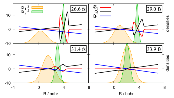
Figure S.4: Time snapshots of the exact density on the first (orange) and second (green) electronic states, nuclear quantum momentum (blue line), and projected quantum momentum (black line) and crunch term (red line) on state 1 during the recoherence event for 3HO model.

References

Kaufman et al. (2023)Brian Kaufman, Philipp Marquetand, Tamás Rozgonyi, and Thomas Weinacht, “Long-lived
electronic coherences in molecules,” Phys. Rev. Lett. 131, 263202 (2023).
Garg et al. (2022)M. Garg, A. Martin-Jimenez, M. Pisarra, Y. Luo,
F. Martín, and K. Kern, “Real-space subfemtosecond imaging of
quantum electronic coherences in molecules,” Nature Photonics 16, 196–202 (2022).
Mogol et al. (2023)Gonenc Mogol, Brian Kaufman,
Chuan Cheng, Itzik Ben-Itzhak, and Thomas Weinacht, “Direct observation of entangled
electronic-nuclear wave packets,” (2023), arXiv:2311.10588 [quant-ph] .
Despré et al. (2018)Victor Despré, Nikolay V. Golubev, and Alexander I. Kuleff, “Charge migration in propiolic acid: A full quantum dynamical study,” Phys. Rev. Lett. 121, 203002 (2018).
Dey et al. (2022)Diptesh Dey, Alexander I. Kuleff, and Graham A. Worth, “Quantum
interference paves the way for long-lived electronic coherences,” Phys. Rev. Lett. 129, 173203 (2022).
Vacher et al. (2017)Morgane Vacher, Michael J. Bearpark, Michael A. Robb, and João Pedro Malhado, “Electron
dynamics upon ionization of polyatomic molecules: Coupling to quantum nuclear
motion and decoherence,” Phys. Rev. Lett. 118, 083001 (2017).
Duan et al. (2017)HG Duan, VI Prokhorenko,
RJ Cogdell, K Ashraf, AL Stevens, M Thorwart, and RJD Miller, “Nature does not rely on long-lived electronic quantum coherence for
photosynthetic energy transfer,” Proc. Natl. Acad. Sci. 114
(2017).
Maiuri et al. (2018)Margherita Maiuri, Evgeny E. Ostroumov, Rafael G. Saer, Robert E. Blankenship, and Gregory D. Scholes, “Coherent wavepackets in the fenna–matthews–olson complex
are robust to excitonic-structure perturbations caused by mutagenesis,” Nat. Chem. 10, 177–183 (2018).
Wasielewski et al. (2020)Michael R. Wasielewski, Malcolm
D. E. Forbes, Natia L. Frank, Karol Kowalski, Gregory D. Scholes, Joel Yuen-Zhou, Marc A. Baldo, Danna E. Freedman, Randall H. Goldsmith, Theodore Goodson, Martin L. Kirk, James K. McCusker, Jennifer P. Ogilvie, David A. Shultz, Stefan Stoll,
and K. Birgitta Whaley, “Exploiting
chemistry and molecular systems for quantum information science,” Nature Reviews Chemistry 4, 490–504 (2020).
Cavaletto et al. (2021)SM Cavaletto, D Keefer,
JR Rouxel, F Aleotti, F Segatta, M Garavelli, and S. Mukamel, “Unveiling the spatial distribution of molecular coherences at
conical intersections by covariance x-ray diffraction signals,” Proc. Natl. Acad. Sci. 118
(2021).
Tully (1990)John C. Tully, “Molecular
dynamics with electronic transitions,” The Journal of Chemical Physics 93, 1061–1071 (1990).
Granucci and Persico (2007)Giovanni Granucci and Maurizio Persico, “Critical appraisal of the fewest switches algorithm for surface
hopping,” The
Journal of Chemical Physics 126, 134114 (2007).
Wang et al. (2016)Linjun Wang, Alexey Akimov, and Oleg V. Prezhdo, “Recent progress in surface
hopping: 2011–2015,” The Journal of Physical Chemistry Letters 7, 2100–2112 (2016).
Crespo-Otero and Barbatti (2018)Rachel Crespo-Otero and Mario Barbatti, “Recent
advances and perspectives on nonadiabatic mixed quantum–classical
dynamics,” Chemical Reviews 118, 7026–7068 (2018), pMID: 29767966.
Subotnik et al. (2016)Joseph E. Subotnik, Amber Jain, Brian Landry, Andrew Petit,
Wenjun Ouyang, and Nicole Bellonzi, “Understanding the surface
hopping view of electronic transitions and decoherence,” Ann. Rev. Phys. Chem. 67, 387–417 (2016).
Esch and Levine (2020)Michael P. Esch and Benjamin G. Levine, “State-pairwise decoherence times for nonadiabatic dynamics on more than two
electronic states,” J. Chem. Phys. 152, 234105 (2020).
Min et al. (2015)Seung Kyu Min, Federica Agostini, and E. K. U. Gross, “Coupled-Trajectory Quantum-Classical Approach to Electronic Decoherence in
Nonadiabatic Processes,” Phys. Rev. Lett. 115, 073001 (2015).
Agostini et al. (2016)Federica Agostini, Seung Kyu Min, Ali Abedi, and E. K. U. Gross, “Quantum-Classical Nonadiabatic Dynamics: Coupled- vs Independent-Trajectory
Methods,” J.
Chem. Theory Comput. 12, 2127–2143 (2016).
Ha et al. (2018)Jong-Kwon Ha, In Seong Lee, and Seung Kyu Min, “Surface Hopping
Dynamics beyond Nonadiabatic Couplings for Quantum Coherence,” J. Phys. Chem. Lett. 9, 1097–1104 (2018).
Villaseco Arribas and Maitra (2023)Evaristo Villaseco Arribas and Neepa T. Maitra, “Energy-conserving coupled trajectory mixed quantum-classical
dynamics,” J.
Chem. Phys. 158, 161105
(2023).
Hunter (1975a)Geoffrey Hunter, “Conditional probability amplitudes in wave mechanics,” Int. J. Quantum Chem. 9, 237 (1975a).
Hunter (1975b)Geoffrey Hunter, “Ionization potentials and conditional amplitudes,” Int. J. Quantum Chem. 9, 311 (1975b).
Hunter (1980)Geoffrey Hunter, “Nodeless wave function quantum theory,” Int. J. Quantum Chem. 9, 133 (1980).
Hunter (1981)Geoffrey Hunter, “Nodeless wave functions and spiky potentials,” Int. J. Quantum Chem. 19, 755 (1981).
Hunter and Tai (1982)Geoffrey Hunter and Chin Chui Tai, “Variational marginal amplitudes,” Int. J. Quantum Chem. 21, 1041 (1982).
Gidopoulos and Gross (2014)Nikitas I. Gidopoulos and E. K. U. Gross, “Electronic non-adiabatic states: towards a density functional theory beyond
the Born–Oppenheimer approximation,” Philosophical Transactions of the Royal
Society of London A: Mathematical, Physical and Engineering Sciences 372 (2014).
Abedi et al. (2010)Ali Abedi, Neepa T. Maitra, and E. K. U. Gross, “Exact
Factorization of the Time-Dependent Electron-Nuclear Wave Function,” Phys. Rev. Lett. 105, 123002 (2010).
Abedi et al. (2012)Ali Abedi, Neepa T. Maitra, and E. K. U. Gross, “Correlated
electron-nuclear dynamics: Exact factorization of the molecular
wavefunction,” J. Chem. Phys. 137, 22A530 (2012).
Agostini and Gross (2021)Federica Agostini and E. K. U. Gross, “Ultrafast dynamics with the exact factorization,” Eur. Phys. J. B 94, 179 (2021).
Villaseco Arribas et al. (2022)Evaristo Villaseco Arribas, Federica Agostini, and Neepa T. Maitra, “Exact Factorization Adventures: A Promising Approach for Non-Bound
States,” Molecules 27, 13
(2022).
Li et al. (2022)Chen Li, Ryan Requist, and E. K. U. Gross, “Energy, momentum, and
angular momentum transfer between electrons and nuclei,” Phys. Rev. Lett. 128, 113001 (2022).
Agostini et al. (2014)F. Agostini, A. Abedi, and E. K. U. Gross, “Classical nuclear motion
coupled to electronic non-adiabatic transitions,” J. Chem. Phys. 141, 214101 (2014).
Abedi et al. (2014)A. Abedi, F. Agostini, and E. K. U. Gross, “Mixed quantum-classical
dynamics from the exact decomposition of electron-nuclear motion,” Europhys. Lett. 106, 33001 (2014).
Min et al. (2017)Seung Kyu Min, Federica Agostini, Ivano Tavernelli, and E. K. U. Gross, “Ab Initio Nonadiabatic Dynamics with Coupled Trajectories: A
Rigorous Approach to Quantum (De)Coherence,” J. Phys. Chem. Lett. 8, 3048–3055 (2017).
Granucci et al. (2010)Giovanni Granucci, Maurizio Persico, and Alberto Zoccante, “Including quantum decoherence in surface hopping,” J. Chem. Phys. 133, 134111 (2010).
Lee et al. (2021)In Seong Lee, Jong-Kwon Ha, Daeho Han, Tae In Kim,
Sung Wook Moon, and Seung Kyu Min, “PyUNIxMD: A Python-based
excited state molecular dynamics package,” J. Comput. Chem. 42, 1755–1766 (2021).
Agostini et al. (Last accessed Oct
2023)Federica Agostini, Emmanuele Marsili, Francesco Talotta, Evaristo Villaseco Arribas, Lea Maria Ibele, and Eduarda. Sangiogo Gil, “G-CTMQC,” (Last accessed Oct
2023).