The M33 Synoptic Stellar Survey. III. Miras and LPVs in griJHK_S

Abstract

We present the results of a search for Miras and long-period variables (LPVs) in M33 using $griJHK_{S}$ archival observations from the Canada-France-Hawai ‘ i Telescope. We use multiband information and machine learning techniques to identify and characterize these variables. We recover $\sim$1,300 previously-discovered Mira candidates and identify $\sim$13,000 new Miras and LPVs. We detect for the first time a clear first-overtone pulsation sequence among Mira candidates in this galaxy. We use O-rich, fundamental-mode Miras in the LMC and M33 to derive a distance modulus for the latter of $\mu=24.629\pm 0.046$ mag.

1 Introduction

The local measurement of the Hubble Constant (H₀) by Riess et al. (2022) differs by $>\!5\sigma$ from the value expected from observations of the Cosmic Microwave Background and Baryon Acoustic Oscillations under the assumption of $\Lambda$CDM (Planck Collaboration et al., 2020). Local measurements of H₀ are often based on Cepheid variables (Cepheids) and Type Ia supernovae (SNe Ia) as primary and secondary distance indicators, respectively. Additional independent primary distance indicators can increase the number of secondary distance indicators or enable new distance ladders to better characterize this tension.

Mira variables (hereafter, Miras) can serve as one of these primary distance indicators. Miras are Asymptotic Giant Branch (AGB) stars that can pulsate in fundamental or overtone modes (Wood & Sebo, 1996) with typical periods ranging from $\sim$100 to $\sim$3,000 days (Soszyński et al., 2005, 2009; Riebel et al., 2010). Mira variability is cyclic, characterized by large peak-to-trough amplitudes at optical wavelengths (historically, photo-visual magnitude amplitude $>2.5$ mag, see Kukarkin et al. 1958; Clayton & Feast 1969; more recently $\Delta I>0.8$ mag, Soszyński et al. 2009) and long-term variations in mean magnitude (Mattei 1997, Whitelock et al. 1997). Miras also vary in the near-infrared (NIR) with smaller amplitudes ($\Delta K_{S}>0.4$ mag, Whitelock et al. 2008). Given their low- to intermediate-mass progenitors ($0.8M_{\odot}<M<8M_{\odot}$; Whitelock 2013), they are common and can be found across all types of galaxies. The Milky Way and the Magellanic Clouds have proven to be prodigious sources of Miras, as revealed by the Optical Gravitational Lens Experiment (OGLE; Udalski et al. 1992) and the MACHO project (Alcock et al., 1993).

Miras are typically classified as Oxygen- or Carbon-rich (hereafter, O- and C-rich) based on the dominance of Oxygen- or Carbon-rich molecules in their spectra, affected by the CNO cycle, helium shell burning, and other internal stellar processes. ¹²C and ¹⁸O in particular can be “dredged up" and raised to the surface of the star (Iben & Renzini, 1983; Kobayashi et al., 2011; Karakas & Lattanzio, 2014). The occurrence of dredge-up events is dictated by stellar mass. In the case of stars with $M>4\ M_{\odot}$, another phenomenon called “hot-bottom burning" (HBB) comes into play. During HBB, the bottom of the convective layer heats up to the point that the CNO cycle is activated with the rare appearance of the Na-Na and Mg-Al cycles. This can affect the transition from O-rich to C-rich for Miras, with some models allowing for C-rich Miras to be converted back to O-rich ones (Hinkle et al. 2016, Whitelock & Feast 2000).

Miras follow tight NIR Period-Luminosity relations (PLRs; Glass & Evans, 1981; Glass & Feast, 1982). In the Large Magellanic Cloud (LMC), O-rich Miras have $K$-band PLRs with low scatter ($\sigma=0.12$ mag; Yuan et al. 2017b) that is comparable to the scatter of Cepheid PLRs in the same band ($\sigma=0.09$ mag; Macri et al. 2015).

O-rich Miras with $P<400$ d have been demonstrated to be useful as extragalactic distance indicators. Yuan et al. (2017a) used $I$-band observations from Macri et al. (2001) and Pellerin & Macri (2011) to identify 1,847 Mira candidates in M33. Their study was extended in Yuan et al. (2018) with sparsely-sampled JHK_S light curves, where they obtained NIR PLRs for O-rich Miras and a distance modulus of $24.80\pm 0.06$ mag for M33.

Huang et al. (2018) used NIR Hubble Space Telescope (HST) observations to identify a sample of 139 O-rich Mira candidates in NGC 4258, which they coupled with LMC Miras to obtain a relative distance modulus that was consistent with Cepheid-based measurements. Huang et al. (2020) used NIR HST observations to identify 115 O-rich Mira candidates in NGC 1559 and determine its distance, in conjunction with the maser distance to NGC 4258 and its sample of Miras. Huang et al. (2020) also presented a Mira-based determination of H₀ within $1\sigma$ of the contemporaneous Cepheid-based value from Riess et al. (2019). The Vera C. Rubin Observatory will soon begin its Legacy Survey of Time and Space (LSST), a decade-long deep time domain survey of $\sim$20,000 sq. deg. in the ugrizY bands (Ivezić et al., 2019). Yuan (2017) transformed LMC Mira PLRs (from $VI$ to $griz$) to estimate that LSST should yield $\sim$200,000 Miras across $\sim$200 galaxies within $\sim$15 Mpc, with $\sim$75 of these yielding upwards of 100 Miras each.

In light of this, detailed characterization of Mira properties in griz would benefit searches for Miras in LSST. Ou et al. (2023) used multiple gri surveys with a baseline of $\sim$18 years to improve the periods of 1,637 previously-discovered Miras in M33. They used transformed O-rich Mira $i$-band magnitudes at maximum light to derive a distance modulus of $24.67\pm 0.06$ mag for M33. They also noted that in order to accurately determine Mira periods, it is vital to obtain full-amplitude light curves, as opposed to relying on samples around maximum light.

In this paper, we present the results of a Mira search using $griz$JHK_S observations of M33 and informed by the results presented in Yuan et al. (2017a) and Yuan et al. (2018).

$\S$2 describes our observations and photometry, $\S$3 lays out our procedure for identifying Mira candidates using NIR information, and $\S$4 describes our attempts to use machine learning methods and LMC long-period variables (LPVs) to identify new Mira candidates.

2 Observations and Data Reduction

2.1 MegaCam and WIRCam Observations

We used archival pipeline-processed optical observations of M33 taken with the MegaCam instrument (Boulade et al., 2003) on the Canada-France-Hawai ‘ i Telescope (CFHT). The observations were acquired as part of proposal IDs 04BF26 (PI Beaulieu) and 04BH98 (PI Hodapp). Results from the former were originally presented by Hartman et al. (2006). The data were obtained using the $gS$, $rS$, $iS$, and $zS$ filters (hereafter griz) with a baseline of roughly one-and-a-half years (August 2003 to January 2005).

MegaCam is a wide-field (1 deg. on a side) optical imager consisting of 36 CCDs with a plate scale of $0\aas@@fstack{\prime\prime}187$ per pixel. Each frame is a mosaic image as a result of the CCD array (see Fig. 1). We split each frame into one image per individual CCD and then sorted the images by band. We visually inspected each image and discarded any unusable ones (e.g., due to poor image quality). This yielded a typical coverage of 29, 27, 28 and 1 nights in $griz$, respectively.

We also used archival pipeline-processed NIR observations of M33 obtained with the Wide-field InfraRed Camera (WIRCam; Puget et al. 2004) on CFHT. The observations were taken as part of three different studies (proposal IDs 06BF36 & 07BF23, PI Beaulieu, $JK_{S}$, 2006-07; proposal ID 15BT03, PI Ngeow, $H$, 2015; proposal ID 17BT02, PI Lee, $H$, 2017-18) and covered different areas within the central disk of M33. The approximate spans of the programs were 1, 2.5 and 1 year, respectively.

WIRCam consists of four detectors with a combined field of view $20\aas@@fstack{\prime}5$ on a side and a plate scale of $0\aas@@fstack{\prime\prime}3$ per pixel (Puget et al. 2004). Each WIRCam frame is effectively a “data cube" comprised of four to five 10-second exposures of the field of view at the time of observation. Each exposure is a mosaic of four images corresponding to each of the chips. We combined the multiple 10-second exposures of a given chip within each frame and only carried out photometry on these composite images. This yielded an average of 9, 6 and 3 epochs in JHK_S, respectively, for locations imaged in a given band.

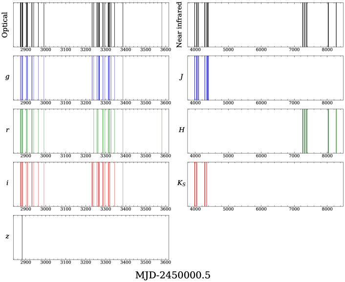
Figure A1: Observations across all optical (top left) and NIR bands (top right), griz (left, top to bottom), and JHK_S (right, top to bottom).

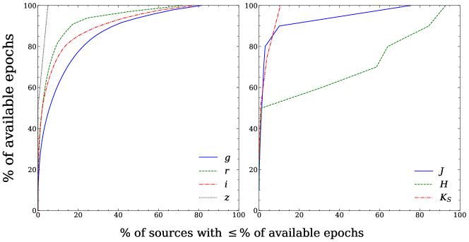
Figure A2: Availability of epochs for sources in griz (left), and JHK_S (right).

The cadence of the MegaCam and WIRCam observations are shown in Fig. A1, while Fig. A2 shows the cumulative distribution of detected sources as a function of the number of the epochs available for that band. As we will show later, our typical Mira candidates had 4, 13, 43, 1, 6, 5 and 2 observations in $griz$JHK_S, respectively.

2.2 Photometry

To process the MegaCam images, we first identified a reference epoch for each band by examining the point-spread functions (PSFs) of stars in the images associated with CCD#11. We chose that detector because it partially covers the disk of M33 at a reasonable source density. None of the reference epochs had any unusable images.

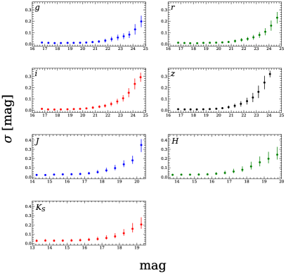
Figure A3: Photometric uncertainties as a function of magnitude, binned in 0.5 mag increments.

We obtained aperture and PSF photometry for all images using DAOPHOT, ALLSTAR, ALLFRAME and related programs (Stetson, 1987, 1994) with a Python wrapper. A primary image for each CCD and band was constructed using MONTAGE. The primary images were then used to create source lists for ALLFRAME. TRIAL (Stetson, 1996) was used to perform frame-to-frame zeropoint corrections, calculate variability statistics, obtain mean instrumental magnitudes, and extract light curves. Sources were then matched across filters for each CCD. The photometric uncertainties versus magnitude for each band are shown in Fig. A3.

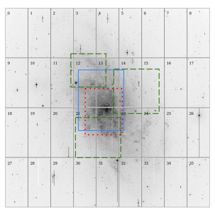
Figure 1: Mosaic of a typical CFHT MegaCam image of M33 with the CCD numbers marked, also showing the areas covered by WIRCam in $J$ (blue, solid), $H$ (green, dashed), and $K_{S}$ (red, dotted) fields. North is up and east is to the left.

We performed the astrometric and photometric calibration of the MegaCam sources using images from the Panoramic Survey Telescope and Rapid Response System (Pan-STARRS) Telescope #1 Data Release 1 (PS1 DR1; Chambers et al. 2016). We solved for the astrometric solution using WCSTools (Mink, 1999) with the primary image of each CCD and filter. Following this, we matched CFHT and PS1 DR1 sources with a tolerance of 2″. If multiple sources satisfied that criterion, the closest Pan-STARRS source was selected.

We used our list of astrometrically-calibrated sources to solve for the following photometric transformations with iterative 2.5$\sigma$ rejection:

$$m_{C}-m_{I}\ =\textrm{ZP}+\chi+\xi(\textrm{col}-\text{piv})$$ (1)

where $m_{C}$ is the fully-calibrated PS1 magnitude, $m_{I}$ is the instrumental magnitude reported by DAOPHOT/ALLSTAR/ALLFRAME (corrected for exposure time), ZP is the MegaCam default zeropoint for a given band, $\chi$ is the residual zeropoint, $\xi$ is the color term, col is the PS1 color, and piv is a “pivot” color value typical of our target stars. We solved for global values of $\xi$ for each transformation, using several thousand stars spanning a wide range of colors, and for chip-specific values of $\chi$ using $\sim$150 stars per CCD, with a typical scatter of 0.04 mag.

To process the WIRCam images, we first identified the fields associated with the various observing programs. There was no consistent overlap across all the frames and filters, as seen in Fig. 1. Before beginning photometry, we separated the images into groups based on their location on the sky (4, 25 and 10 groups for $JHK_{S}$, respectively). Reference images for each group were chosen by visual inspection. We then obtained aperture and PSF photometry for the WIRCam images using the same methods as for the MegaCam images.

We performed the astrometric and photometric calibration of the WIRCam sources using the catalog from Javadi et al. (2015), based on observations with the UK InfraRed Telescope (UKIRT). We used the WIRCam WCS information for a preliminary match against the UKIRT catalog, finding global offsets of $0.5-1.5\arcsec$ (depending on the band) and correlated residuals as a function of position. These are likely due to different geometrical distortions in the two cameras and were removed using second or third-order polynomials. The remaining residuals were removed using a non-parametric technique. We divided each image in $100\times 100$ pixel cells and used the average residuals of the stars in each cell to fit a thin-plate spline and apply the necessary correction. The final dispersion of position residuals after all corrections was $\sim 0\aas@@fstack{\prime\prime}1$. All corrections done after the initial global offset were based on the 5,000 brightest stars in a given image.

We solved for the the NIR photometric transformations using the following equation with iterative $2.5\sigma$ rejection:

$$m_{I}-m_{C}\ =\chi\ +\xi(J-K_{S}-1.0)\ +\xi^{{}^{\prime}}(J-K_{S}-1.0)^{2}$$ (2)

where $m_{I}$ is the instrumental magnitude, $m_{C}$ is the calibrated UKIRT magnitude, $\chi$ is the residual zeropoint, $\xi$ and $\xi^{{}^{\prime}}$ are the first- and second-order color terms and $J-K_{S}$ is the UKIRT color. We solved for global parameters across the four detectors.

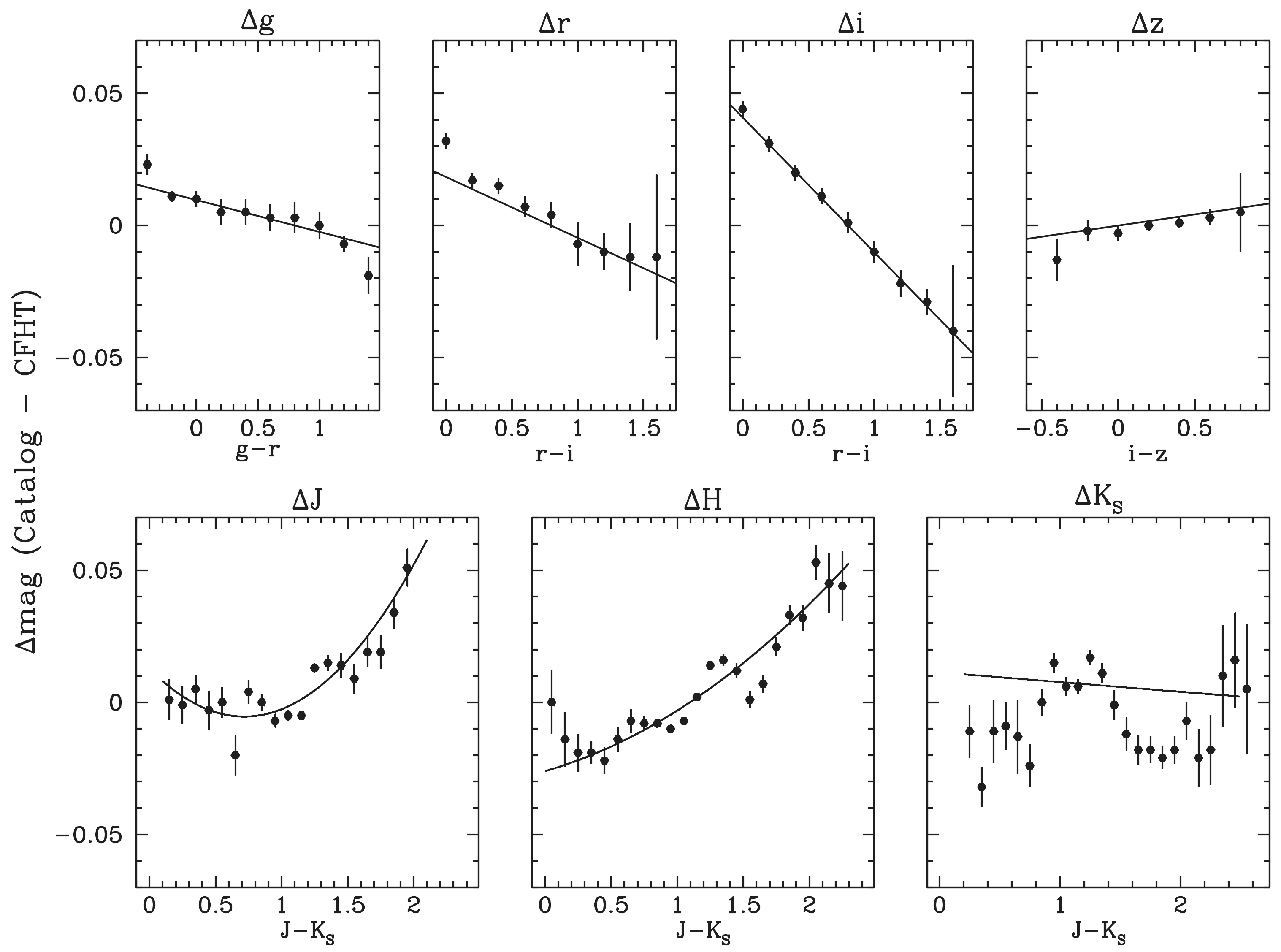
Figure A4: Representative photometric transformations for all bands. Symbols are binned residuals while solid lines represent the best-fit color terms.

The mean values of all coefficients in the photometric transformations are presented in Appendix Tables A1 and A2, and representative solutions are shown in Fig. A4. These were applied to all stars in our catalog, including those lying outside of the color range spanned by the local standards. We fully propagated the uncertainties in all transformation coefficients, which for our objects of interest never exceeded 0.03 mag.

Appendix Table A4 presents the fully-calibrated time-averaged magnitudes in all available bands for all $\sim$1.15 million point sources detected in our analysis, as well as their $gri$ variability statistics.

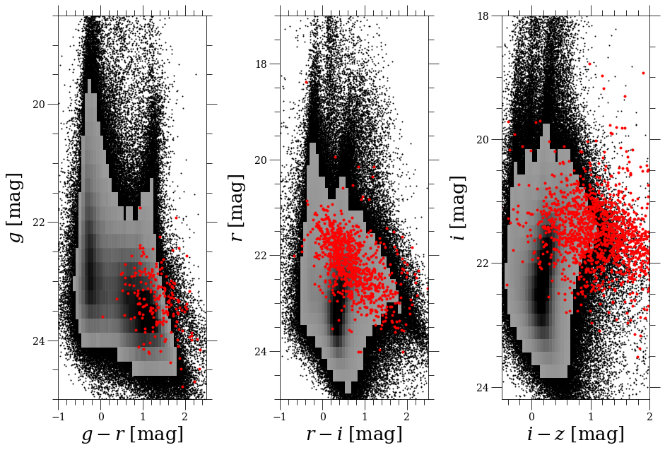
Figure 2: Hess diagrams in the optical bands. Individual stars are plotted where the source density drops below 200 objects per bin. Recovered Miras from Yuan et al. (2017a) are shown using red points. Mira recovery varies across filters. Not all recovered Miras were kept in our final samples, due to quality cuts.

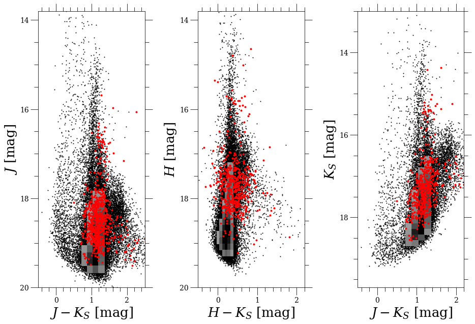
Figure 3: Same as Fig. 2, but for the NIR bands.

2.3 Crowding corrections

Biased magnitude measurements have long been recognized as an issue affecting crowded-field photometry of faint stars (McClure et al., 1985; Stetson, 1987; Schechter et al., 1993). The standard approach to characterizing and correcting this bias relies on the injection of artificial stars in the vicinity of, and with the same flux as, the objects of interest. Only a few artificial stars should be added around a given object, in order to mitigate any further crowding of the image.

Following these precepts, we created 20 copies of each $JHK_{S}$ primary image and in each one we added 5 artificial stars to the vicinity of each of the 14,312 variables described in §3.

The radial distances between artificial stars and their corresponding variables were drawn from a uniform random distribution spanning 5-12 pix (1.5-3.6″). Every artificial star in a given copy of a primary image had to be at least 4 pix (1.2″) away from each other and from every Mira candidate or other stars in the frame (down to 2 mag fainter than the corresponding source of interest).

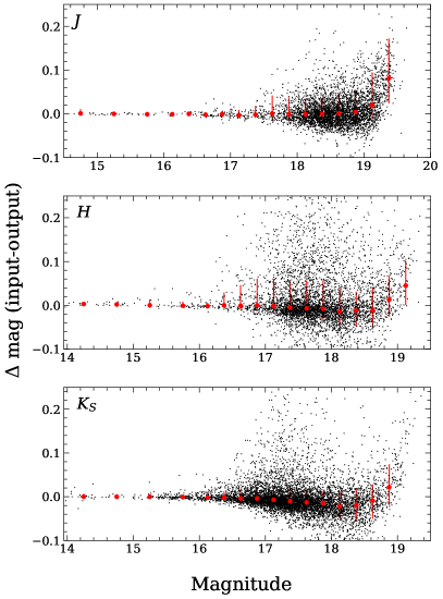
Figure A5: Results of artificial star tests to characterize the crowding bias in the NIR photometry of LPVs and Mira candidates. Small black dots represent the error-weighted mean crowding correction for each object. Larger red filled symbols show median values and red errorbars depict $\pm 1\sigma$ ranges for stars in each bin.

We carried out the same photometric procedures on each of the artificial images as previously done in the real ones, identified the artificial sources and compared the recovered and input magnitudes. The results are shown in Fig. A5. Crowding corrections are minimal for objects with $m<$19: $0.014\pm 0.054$ ($J$), $0.009\pm 0.067$ ($H$), $-0.002\pm 0.042$ ($K_{S}$). $\sim 22$% of the variables had crowding corrections exceeding 0.1 mag or uncertainties in those corrections beyond 0.1 mag; they were flagged accordingly and excluded from the final samples.

3 Identifying LPVs and Mira Candidates Using Optical and NIR Observations

3.1 Initial selection

We identified $\sim$1.15 million unique objects from our photometry which had at least one detection in one of the $gri$ bands. The Hess/color-magnitude diagrams for the optical and NIR bands are shown in Figs.  2 and 3 respectively, with the recovered Miras from Yuan et al. (2017a) and Yuan et al. (2018) overplotted.

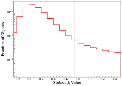
Figure A6: Histogram of Stetson $J$ variability index values for all sources detected in $i$ (step 2 of Table A3). The vertical dashed line at $J_{i}=0.75$ is the threshold we adopted.

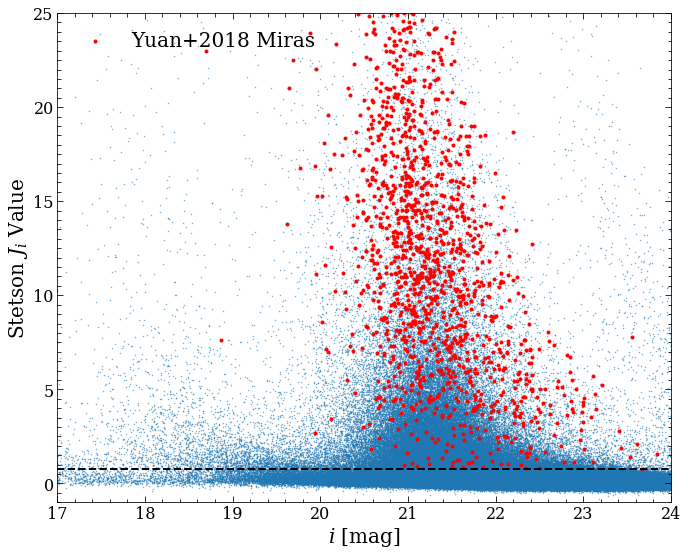
Figure A7: $J_{i}$ versus $i$ for all sources detected in that band (step 2 in Table A3). The horizontal dashed lined at $J_{i}=0.75$ shows the adopted threshold. Recovered Miras from Yuan et al. (2018) are overplotted in red.

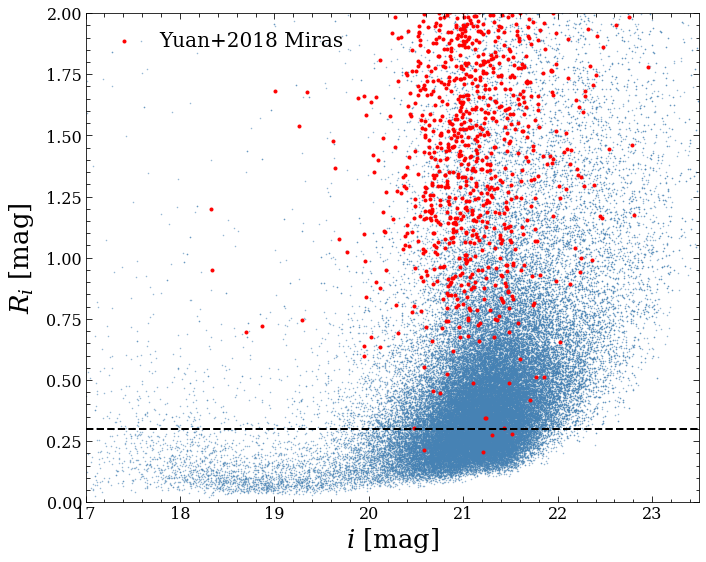
Figure A8: Range of magnitudes spanned by $i$ light curves ($R_{i}$) versus mean $i$ magnitude for objects with: (i) $J_{i}\geq 0.75$, (ii) $r-i\geq 0$ or a non-detection in $r$. The horizontal dashed line shows our adopted threshold of $R_{i}\geq 0.3$. The Miras from Yuan et al. (2018) are overplotted in red.

We began the selection of LPVs and Mira candidates by making variability, color, and amplitude cuts based on the optical data. The variability cuts were based on the Stetson $J$ index (Stetson, 1996) calculated from our $i$ band measurements ($J_{i}$) using TRIAL. This index takes into account correlated deviations from a mean magnitude and their measurement quality; the higher its value, the more likely an object is genuinely variable. We only considered objects with $J_{i}\geq 0.75$, which corresponds to a $\sim$5$\sigma$ detection of variability using this index. Fig. A6 presents a histogram of $J_{i}$ values while Fig. A7 shows $J_{i}$ versus $i$. As the next step, since Miras are red variables, we only considered objects with either $r-i\geq 0$ or a non-detection in the $r$ band. Among the remaining objects, we selected those whose $i$-band light curves spanned a range ($R_{i}$) of at least 0.3 mag (see Fig. A8 for the overall distribution of this parameter). We selected this threshold as it only excluded $\sim$1% of the previously-known Mira candidates recovered by our photometry.

We then selected the objects that were detected in at least three epochs in one of the NIR bands, as that information is needed for our subsequent analysis. Following all the stated cuts (summarized in Table A3), we were left with 14,312 variables, which included 1,342 of the Miras identified in Yuan et al. (2018).

3.2 Light curve fits

We fit the available griJHK_S light curves of these variables using a simple sinusoidal model, defined for a given band as

$$m(t_{i})\ =\ \overline{m}\ -\ A\sin({2\pi}t_{i}/{P}+\phi)$$ (3)

where $m$ is the magnitude at time $t_{i}$, $\overline{m}$ is the mean magnitude, $A$ is the semi-amplitude, $P$ is the period, and $\phi$ is a phase offset. Since the $z$ measurements were obtained on a single night, they were not considered further in the analysis. We simultaneously fit light curves from several bands using MPFIT (Markwardt, 2009); the values of $\overline{m}$, $A$ and $\phi$ might be different for each band but $P$ was always solved for as a common parameter. We fit each variable using 55 trial periods equally spaced every $0.02\log P$, spanning $1.925\leq\log P\leq 3.005$, and selected the fit with the lowest $\chi^{2}_{\nu}$.

We attempted to fit the light curves using modern techniques, such as the semi-parametric Gaussian Process model (Yuan et al., 2017a; He et al., 2016) and stochastic variational inference models (He et al., 2021) that have been used recently on longer Mira time series. Unfortunately, the limited number of cycles covered by our data and the lack of time overlap between the optical and the NIR bands hampered the performance of these models.

We initially fit only the $iJHK_{S}$ light curves for the 1,342 recovered Miras from Yuan et al. (2017a), solving for independent values of $\overline{m}$, $A$ and $\phi$. Using objects from this subsample with information in at least two NIR bands, we found $A_{H}\sim$ $A_{J}$, $A_{K_{S}}\sim$ $0.9A_{J}$, $\phi_{H}\sim$ $\phi_{J}$ and $\phi_{Ks}\sim$ $\phi_{J}-0.03$, which we adopted for the subsequent analysis. This simplification was motivated by the relatively small number of data points per light curve in the NIR bands.

Having implemented the above interrelations for NIR amplitudes and phases, we next expanded the fit to all six bands for objects in this subsample. We further derived $\phi_{r}\sim\phi_{i}+0.015$ and $\phi_{g}\sim\phi_{i}+0.03$, which we also adopted for the subsequent analysis. We did not find useful interrelations for the amplitudes in $gri$, nor could we find a robust global offset between $\phi_{i}$ and $\phi_{J}$.

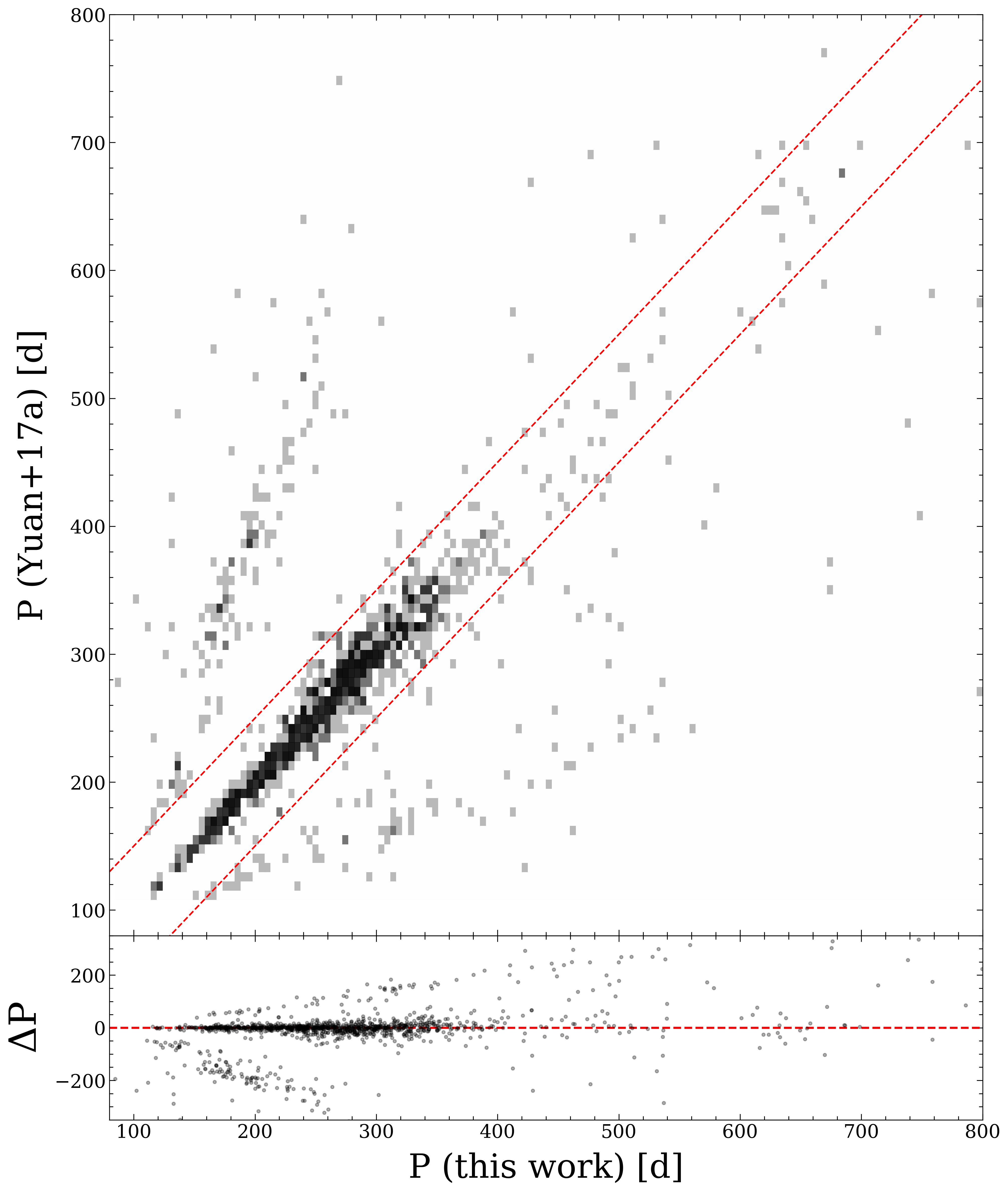
Figure A9: Top: Comparison of periods for Mira candidates from Yuan et al. (2017a) that were recovered in this work; $\sim$78.1% of them had $\Delta P/P<50$ d. Bottom: Residuals from the 1:1 relation.

Fig. A9 compares the periods of objects in this subsample derived by Yuan et al. (2017a) and by our procedure. We found good agreement (defined as $\Delta P<50$ d) for $\sim$78.1% of the objects, with most of the others lying along the $\pm 1/365$ d alias relations. This recovery rate is very similar to the one found by Yuan et al. (2018) based on simulations of Mira light curves with similar sampling to our work. Since our fitting procedure did not return $\sigma(P)$ for all objects, we used the scatter about this 1:1 relation to determine $\langle\sigma({\Delta P}/{P})\rangle=0.03$. We only used our best-fit periods in all subsequent analysis.

We fit the coupled sinusoidal model to all 14,312 variables (using the same set of trial periods described above) to derive $P$ for each object and the following properties (when available): up to six mean magnitudes ($griJHK_{S}$), four amplitudes ($A_{g},A_{r},A_{i}$ and $A_{JH}$, with $A_{K_{S}}$ coupled to the latter), and two phases ($\phi_{i}$ and $\phi_{JH}$, with $\phi_{g}$ and $\phi_{r}$ coupled to the former and $\phi_{Ks}$ coupled to the latter). Fig. 4 shows the light curves and best-fit model for a recovered Mira.

Once mean magnitudes had been obtained, we calculated NIR Wesenheit indices (Madore, 1982), defined as

$$W_{JK_{S}}=K_{S}-R_{JK_{S}}^{K}(J-K_{S});\ \ \ W_{JH}=H-R_{JH}^{H}(J-H),$$ (4)

which simultaneously minimize the effects of temperature and extinction. We adopted $R_{JK}^{K}=0.742$ and $R_{JH}^{H}=1.727$, calculated as in Yuan et al. (2018) using Schlafly & Finkbeiner (2011) values.

Appendix Table A7 presents the properties and associated uncertainties of all 14,312 LPVs, as well as the machine-learning classification scores and other labels to be described in §4.

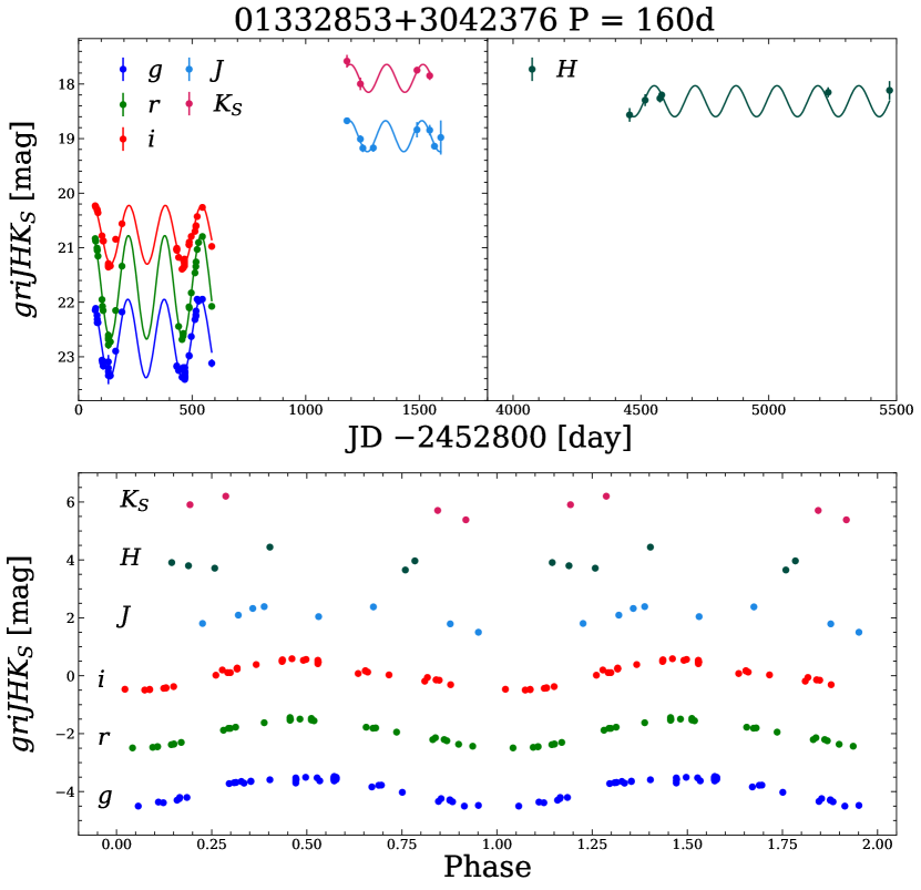
Figure 4: A representative Mira from our sample that was previously identified by Yuan et al. (2017a). Upper panel: observed light curves in $griJHK_{S}$. Lower panel: phased light curves; magnitudes have been offset and two cycles are plotted for clarity.

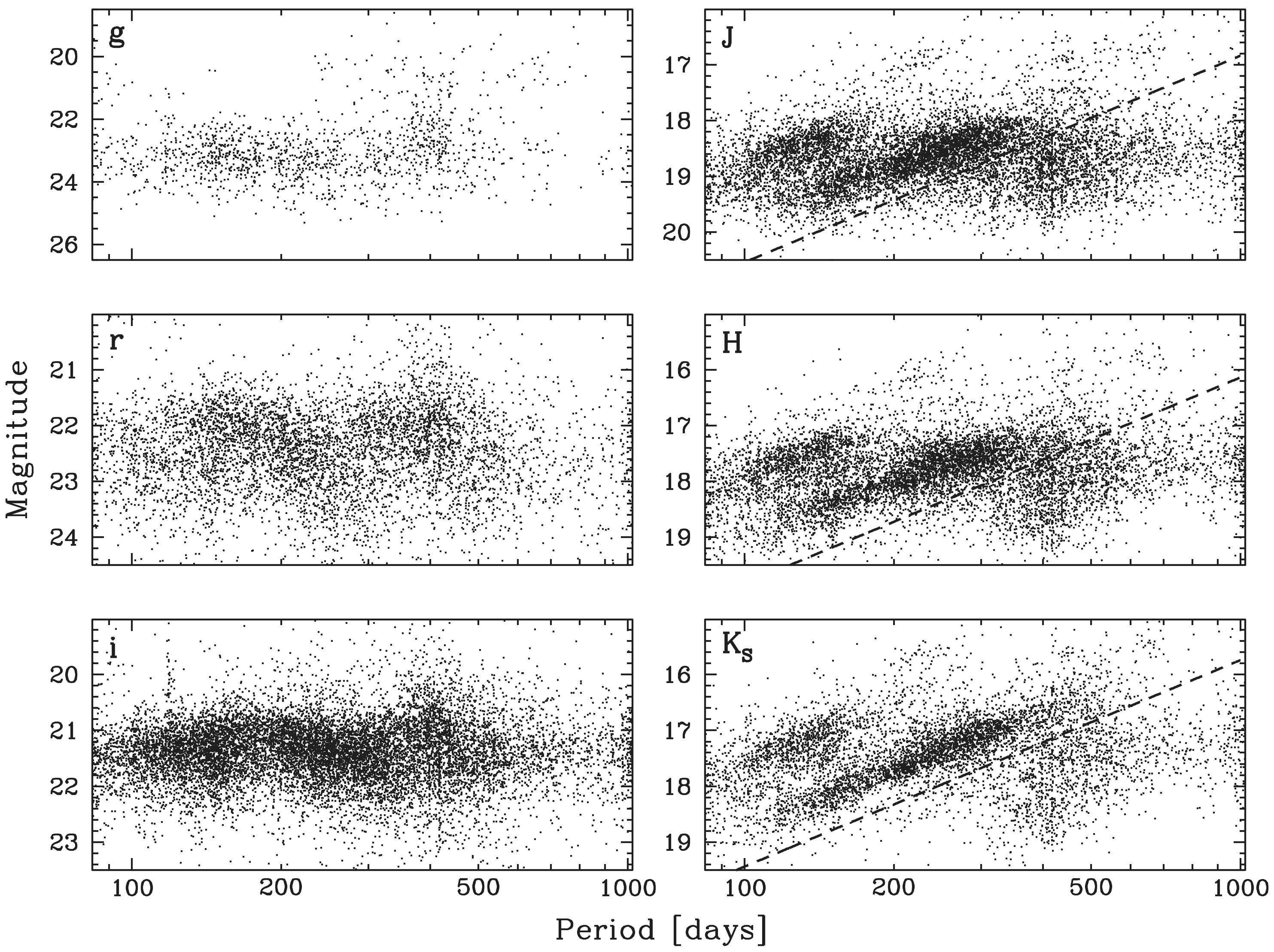
Figure 5: Period-magnitude diagrams of LPVs in M33 identified in our analysis. Left column, top to bottom: $g$, $r$, $i$. Right column, top to bottom: $J$, $H$, $K_{S}$. The dashed lines on the right panels indicate the limits used to separate faint objects from first-overtone and fundamental pulsators.

Figs. 5 and 6 show the resulting period-magnitude and period-Wesenheit diagrams. Two obvious sequences can be seen in all the NIR relations, with $K_{S}$ magnitudes of $\sim$ 16.8 and 18.1 at $\log P=2.2$. These correspond to first-overtone (FO) and fundamental-mode (FU) pulsators, respectively, as first identified in the LMC by Wood & Sebo (1996). A third much more diffuse group (which we labeled FA for “faint") can be seen at $\log P\gtrsim$2.6 and $K_{S}\gtrsim$17, becoming somewhat more obvious in the Wesenheit relations. Most of these objects have smaller values of $A_{i}$ compared to those in the other sequences, and may be the counterparts of the LMC LPVs plotted in green and lying below (fainter than) sequence D in Fig. 1 of Soszyński et al. (2013).

3.3 Classification into O- and C-rich subtypes

As previously mentioned, O-rich Miras have been shown to obey tighter Period-Luminosity relations than their C-rich counterparts. Thus, it is of interest to classify Miras into subtypes in order to obtain better distance estimates. In the absence of spectroscopic observations, which would be prohibitive to obtain for large extragalactic samples, this classification must rely on photometric information.

The LMC is an ideal system to derive photometric-based classification methods for Miras given the better quality light curves that can be obtained for its variables. Soszyński et al. (2005) combined their OGLE-II/III $V$ and $I$ photometry of LPVs with 2MASS PSC Cutri et al. (2003) $JHK_{S}$ magnitudes to derive Period-Luminosity relations of Miras and semi-regular variables (SRVs) in this system. They showed that these two types of pulsators follow the C and C^′ sequences, respectively, originally identified by Wood & Sebo (1996) and later characterized by Ita et al. (2004).

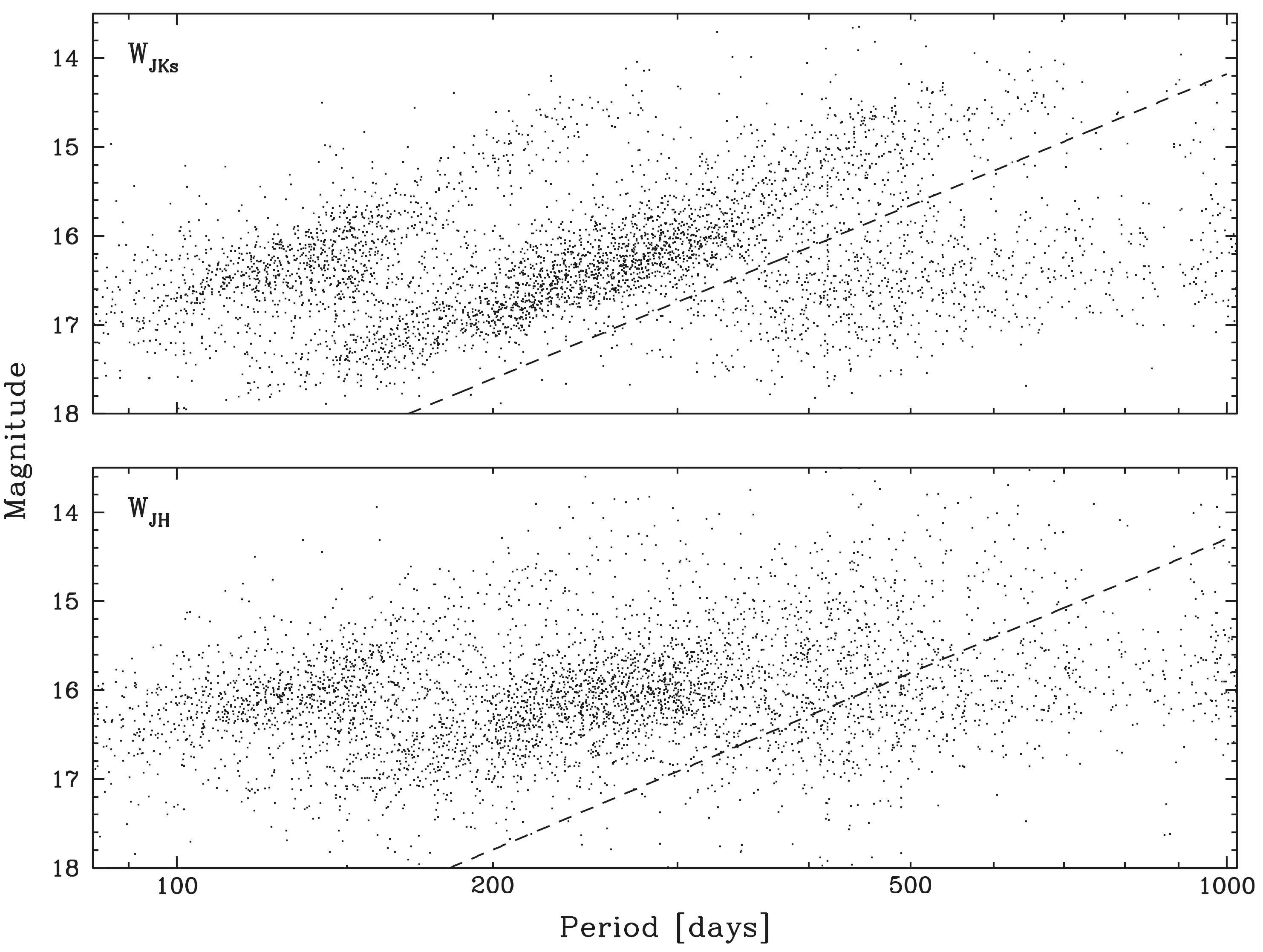
Figure 6: Same as Fig. 5, but using NIR Wesenheit indices.

Soszyński et al. (2009) presented a catalog of OGLE-III LMC LPVs based on optical observations that consists of 1,667 Miras and 11,128 SRVs. They combined their measurements with 2MASS NIR magnitudes to show that Miras can be reliably separated into O- and C-rich types in the $V-I$ vs. $J-K_{S}$ plane, or by comparing optical and near-infrared Wesenheit indices. Yuan et al. (2018) also showed that O- and C-rich Miras can be separated well in the $J-H$ vs. $H-K_{S}$ plane. Menzies et al. (2019) studied AGB variables in NGC 3109 and showed that a simple cut in $J-K_{S}$ is not a reliable method to separate O- and C-rich Miras due to changes in color as a function of abundance.

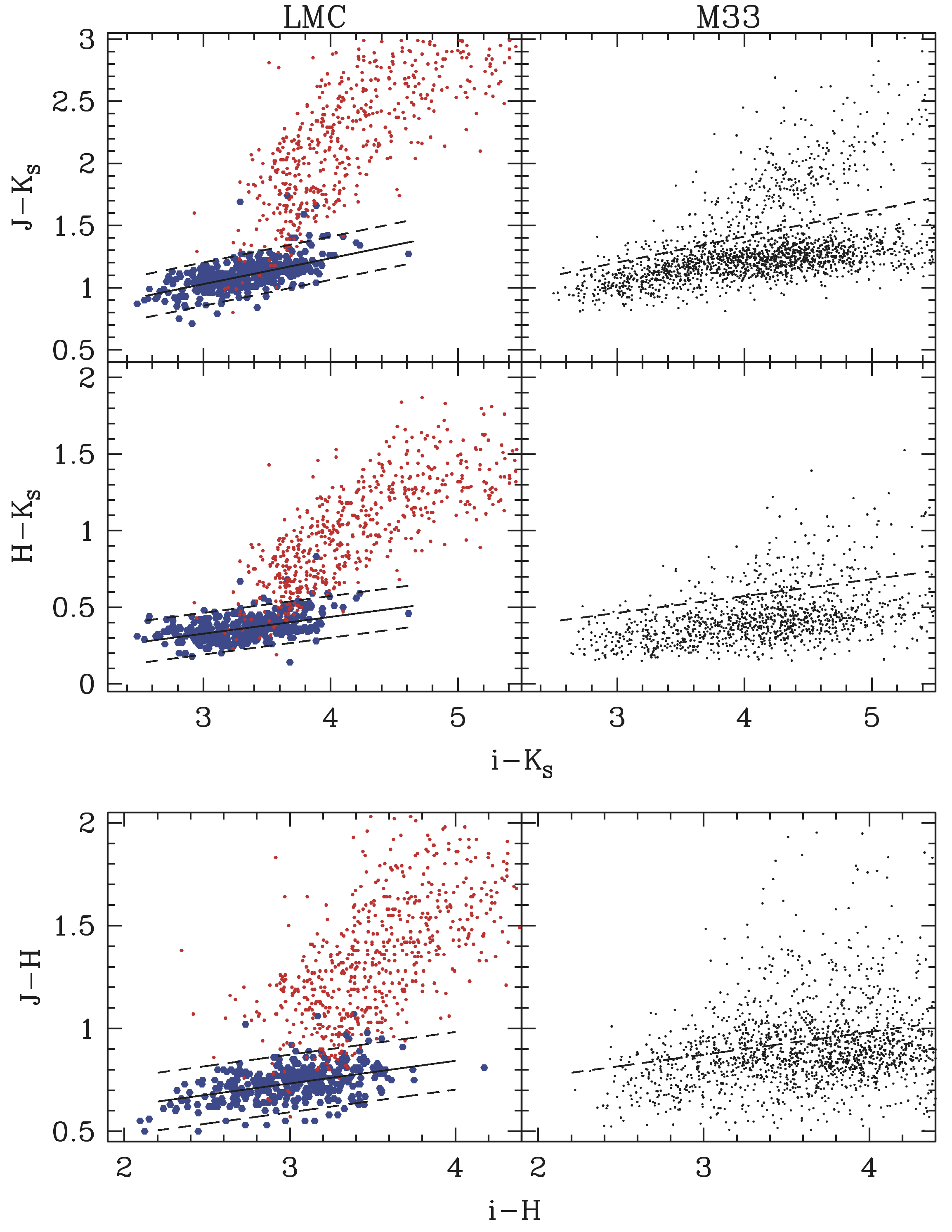
Figure 7: Left: Color-color relations of OGLE-III Miras in the LMC. Blue and red red symbols indicate O- and C-rich variables, respectively. The solid lines are the best-fit linear relations of O-rich objects, with dashed lines indicating the $\pm 2\sigma$ dispersion. Right: Same relations for our final M33 samples, with dashed lines indicating the division between O- and C-rich variables.

Color	Relation	$\sigma$
$J-K_{S}$	1.028 + 0.209 $(i-K_{S}-3)$	0.087
$H-K_{S}$	0.327 + 0.110 $(i-K_{S}-3)$	0.068
$J-H$	0.733 + 0.110 $(i-H-3)$	0.070

Table 1: Color-color relations of LMC O-rich Miras, used to classify M33 variables.

Regrettably, given the nature of the archival observations of M33 that form the basis of our study, we do not have $I$ magnitudes (but have $i$ instead), only a very small fraction of Miras have $g$ magnitudes, and there is little overlap between the $J/K_{S}$ and $H$ observations. Fortunately, we have $iJK_{S}$ magnitudes for the vast majority of objects.

We cross-matched the OGLE-III LMC Miras with the near-infrared catalog of Kato et al. (2007), which is significantly deeper and has considerably better angular resolution than 2MASS, to obtain improved $JHK_{S}$ magnitudes. We used the BaSTI stellar evolution database (Pietrinferni et al., 2013; Pietrinferni et al., 2021) to derive cubic relations between $I-JHK_{S}$ and $i-JHK_{S}$ colors for RGB and AGB stars, so that we could directly compare the LMC and M33 relations. We used the existing OGLE classification of these Miras into O- and C-rich types to generate the diagrams shown on the left-hand side of Fig. 7. The O-rich Miras delineate tight sequences in the various color-color relations, which are listed in Table 1, with a scatter of $\sim 0.07$ mag.

We used the $+2\sigma$ ridge of the LMC $(i-K_{S},J-K_{S})$ color-color relation (top-left panel of Fig. 7) delineated by the O-rich Miras as our primary method to classify the M33 variables. If $J$-band photometry was not available, we used the equivalent ridge in the LMC $(i-K_{S},H-K_{S})$ relation (middle-left panel of the same Figure). If $K_{S}$ band photometry was not available, we used the $+3\sigma$ ridge of the LMC $(i-H,J-H)$ relation (bottom-left panel of the same figure) to account for additional dispersion in the M33 sample. If only one NIR band was available, no classification was done.

4 Identifying New Mira Candidates

We identified new Mira candidates out of our LPV sample using two approaches. The first one relies on machine-learning techniques applied to our $i$ light curves, while the other one uses near-infrared Period-Luminosity relations of Miras in the Large Magellanic Cloud. We then derived period-Wesenheit relations for the newly-selected Mira candidates and the previously-known ones.

We applied several quality cuts to the 12,970 LPVs not previously classified as Miras before carrying out these procedures. The cuts were applied consecutively and resulted in the rejection of the following numbers of variables:

1. 2,891 with crowding corrections or uncertainties in these corrections exceeding 0.1 mag;

2. 1,336 with best-fit periods near the lower or upper limits of our grid search ($\log P<$2 or $\log P>$3);

3. 296 with abnormally blue colors (any of $J\!-\!K_{S}<$0.8, $H\!-\!K_{S}<$0.2, $J\!-\!H<$0.5, $i\!-\!H<$2, $i\!-\!K_{S}<$2.5);

4. 2,303 faint variables lying below the first-overtone and fundamental mode groups, identified as follows. The dividing lines are also plotted in Figs. 5 and  6.

   • 783 with $W_{JK_{S}}>18.0\!-\!4.9\ (\log P\!-\!2.2)$;

   • 332 with $W_{JH}>18.0-4.9\ (\log P\!-\!2.2)$;

   • 262 with no $J$ or $H$ data and $K_{S}>18.6\!-\!3.7\ (\log P\!-\!2.2)$;

   • 532 with no $J$ or $K_{S}$ data and $H>19.1\!-\!3.7\ (\log P\!-\!2.2)$;

   • 394 with no $H$ or $K_{S}$ data and $J>19.8\!-\!3.7\ (\log P\!-\!2.2)$

which resulted in a classification sample of 6,144 variables. These cuts were also applied to the recovered Miras from Yuan et al. (2018); 934 out of 1,342 were selected for further analysis.

4.1 Machine Learning Classification

We used six machine learning methods as classifiers to identify new Mira candidates: logistic regression, random forest, linear discriminant analysis, quadratic discriminant analysis, kernel support vector machine (SVM), and positive-unlabeled learning with bagging SVM (Mordelet & Vert, 2014). All six of the methods work as binary classifiers, which is ideal for our goal of distinguishing Miras from other types of variables. We set up the classifiers so that each one returned a score for each object; the higher the value, the more Mira-like.

Feature	Description	Source	Rank
$\sigma(R_{q})/$	Ratio of std deviations,	L	2
$\sigma(\overline{m})$	defined below
$R_{0.9}$	Light curve range from	L	3
	10th to 90th percentile
$R$	Light curve range	L	5
$A_{P}$	Semi-amplitude of periodic component	M	6
$\sigma(\overline{m})$	Std dev of residuals about unweighted	L	8
	mean magnitude, $\overline{m}$
$\sigma(R_{q})$	Std dev of residuals from piece-	M	10
	wise quadratic fits∗

Table 2: Classifier features used to identify new Mira candidates, based on Yuan et al. (2017a) and listed according to their rank in that publication.
L: light curve; M: model. *: $\sigma(R_{q})$ was not used as a stand-alone parameter; it is only described to define $\sigma(R_{q})/\sigma(\overline{m})$.

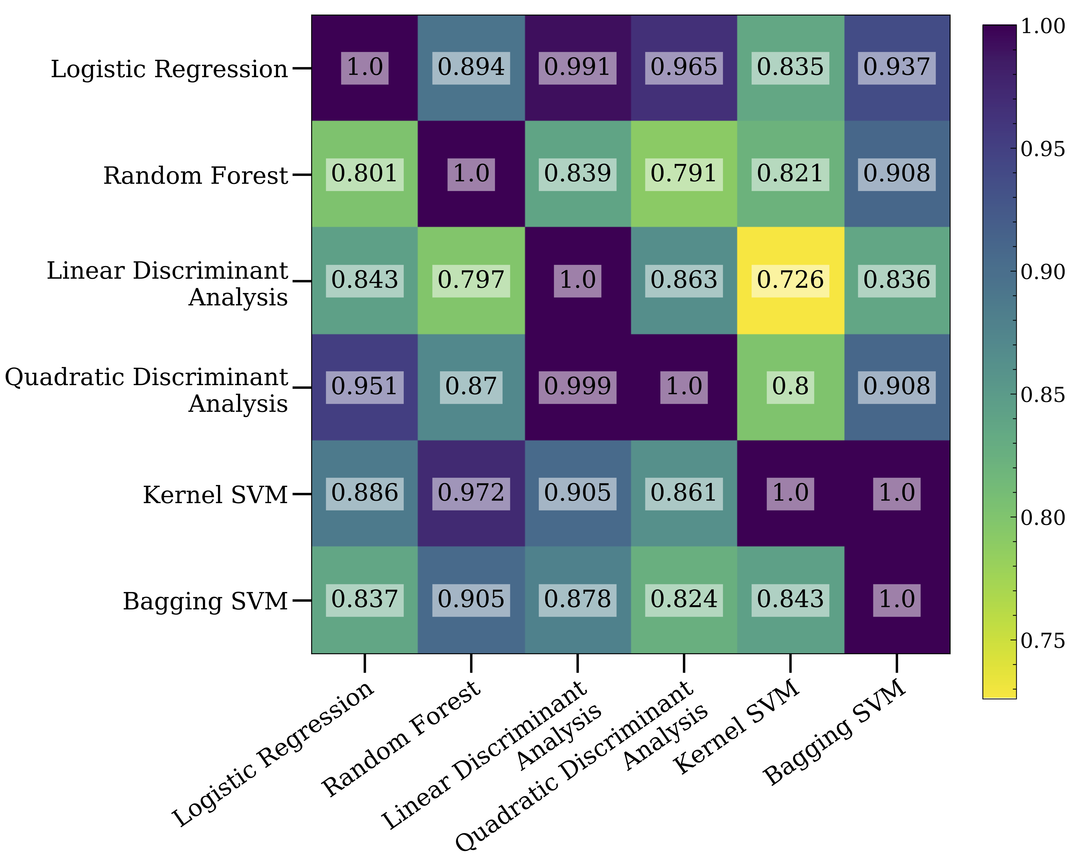
Figure 8: Fraction of common candidates across the samples returned by the six machine learning classifiers.

The classifiers were provided with the first five features described in Table 2, which are associated with the $i$-band light curves and best-fit models. These features were amongst those used to identify Mira candidates in Yuan et al. (2017a). We could not include other features from that work because they require periodograms, which our simple sinusoidal fit could not provide.

We trained and validated the classifiers using the Mira candidates from Yuan et al. (2018) that we recovered in our data, as well as the objects that did not pass sample cuts #1-5 described in §3 and Table A3. The former were considered as known Miras while the latter were considered as known non-Miras.

After training and validating the classifiers, we used the scores assigned to the validation Miras and non-Miras to create Receiver Operating Characteristic (ROC) curves and determine a threshold for each classifier that would separate Miras from non-Miras. The threshold for each method was determined by maximizing the geometric mean, which is defined as $\sqrt{\text{sensitivity}\times\text{specificity}}$. Using the geometric mean to determine the Mira/non-Mira threshold allows for a balance between classifier performance on both the majority and minority classes. It also avoids overfitting the negative class (non-Miras) and under-fitting the positive class (Miras). The Mira/non-Mira thresholds and area under the ROC curve (AUC) for each classifier are shown in Table A5.

We selected a sample of Mira candidates for each classifier by retaining the objects with a classifier score greater than or equal to the respective Mira/non-Mira threshold. We visually inspected the light curves of every variable identified as a Mira by at least one classifier ($\sim$53% of the remaining sample) and labeled each object as high, low, or no confidence. We retained only the high-confidence objects, which consisted of $\sim$94% of the remaining objects. Table A6 gives the initial number of candidates associated with each classifier and the number that remained after visual inspection. The fractions of initial candidates in common across classifiers are shown in Fig. 8. We define “bronze”, “silver” and “gold” Mira candidate samples as those identified by one, three or all six classifiers, respectively.

4.2 P-L relations from the Machine-Learning Samples

We fit Period-Luminosity relations to various subsets of the 3,052 newly-classified and visually-inspected Mira candidates and the 934 recovered Miras that passed the selection criteria described in §4. We considered both linear and quadratic relations, defined as:

$$m\ =\ a_{0}\ +\ a_{1}(\text{log}_{10}P-2.3)\ [\ +\ a_{2}(\text{log}_{10}P-2.3)^{2}\ ]$$ (5)

and performed error-weighted fits with iterative 2.5$\sigma$ clipping. The photometric uncertainties were rescaled to obtain $\chi^{2}_{\nu}$=1 for each linear fit. The same scaling factor was applied to the corresponding sample prior to performing the equivalent quadratic fit. Results for the latter are only reported if $a_{2}$ was detected at $\geq$4$\sigma$ significance and its inclusion led to a reduction in $\chi^{2}_{\nu}$.

We defined subsamples according to type (O-, C-rich, or all), pulsation mode (fundamental or first overtone), and classifier output. The O/C-rich classification has already been described in §3.3. We adopted the following dividing lines between first-overtone and fundamental mode pulsators:

• $W_{JK_{S}}=$16.7$-6.0\ (\log P-2.2)$;

• $W_{JH}={16.7}$-${6.0}$$\ (\log P-2.2)$;

• $K_{S}=17.6-5.0\ (\log P-2.2)$;

• $H=17.8-4.5\ (\log P-2.2)$;

• $J=18.7-4.5\ (\log P-2.2),$

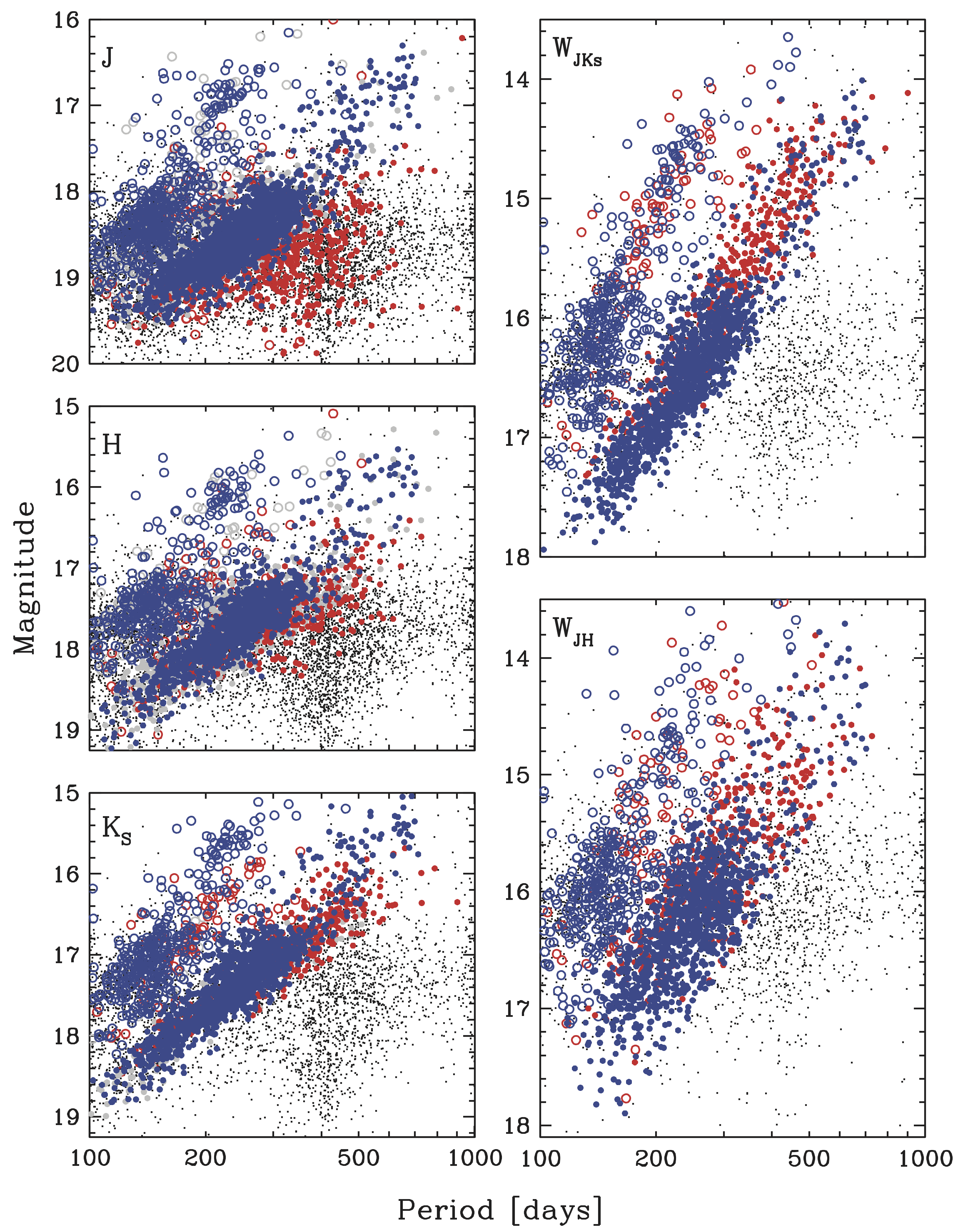
Figure A10: P-L relations in NIR bands and Wesenheit indices for the 3,986 Mira candidates described in §4.2. Variables that did not pass the cuts are plotted using small points. Open and filled circles denote first-overtone and fundamental-mode pulsators. Objects plotted in red and blue were classified as C- or O-rich, respectively, while those in grey only have measurements in one NIR band and thus cannot be classified.

first classifying objects with $W_{JK_{S}}$ indices, then those with only $W_{JH}$ information, and so on. In this way, 3,986 variables were classified as either first overtone or fundamental mode, while 2,709 were classified as either O- or C-rich. Figs. A10-A12 show the resulting P-L relations in the NIR bands and the Wesenheit indices.

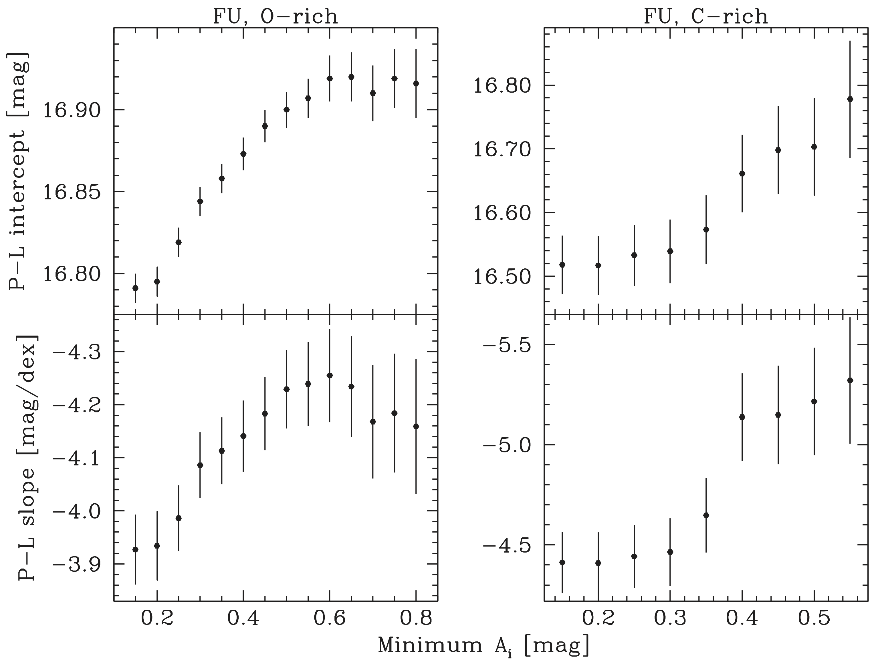
Figure A13: Result of linear fits to the $W_{JK_{S}}$ P-L relations of fundamental-mode pulsators as a function of minimum $i$-band amplitude. Left: O-rich, $P<$400 d. Right: C-rich. Top: P-L intercepts. Bottom: P-L slopes. We adopt a minimum value of $A_{i}=0.5$ mag for our final fits.

We first focused on the $W_{JK_{S}}$ relation for the fundamental-mode O-rich Miras with $P\!<$400 d, which have been widely used for distance determination and exhibit the tightest scatter (Yuan et al., 2018; Huang et al., 2018, 2020). We performed a series of linear fits using increasingly larger values for the minimum semi-amplitude of the light curves in the $i$-band. The results, shown in Fig. A13, indicate a clear trend in zeropoint and slope until $A_{i}\sim 0.5$ mag. A similar trend was seen for fundamental-mode C-rich Miras, and to some extent in the first-overtone samples, although the smaller size of these samples result in noisier results and the latter do not typically reach such large amplitudes. Thus, for the final fits we required $A_{i}>0.5$ and 0.3 mag for fundamental-mode and first-overtone pulsators, respectively.

Table 3 presents the results of all P-L fits, while Fig. 9 shows selected results for our “baseline” samples. In agreement with previous studies, we find the O-rich, fundamental-mode relations exhibit the lowest scatter for a given band or Wesenheit index. In the absence of O/C classification, the resulting fundamental-mode relation usually exhibits a comparable scatter to its O-rich counterpart but it requires a quadratic term. The $K_{S}$ relations exhibit lower or similar scatter to their $W_{JK_{S}}$ counterparts, with the $J$ ones being nearly as good. The $H$ relations exhibit slightly worse scatter than the other two bands, while $W_{JH}$ appears markedly worse than the rest.

We do not find a significant improvement when moving from the baseline “bronze” sample to the “silver” and “gold” ones, which is not surprising given the high degree of correlation among the samples identified by the different classifiers.

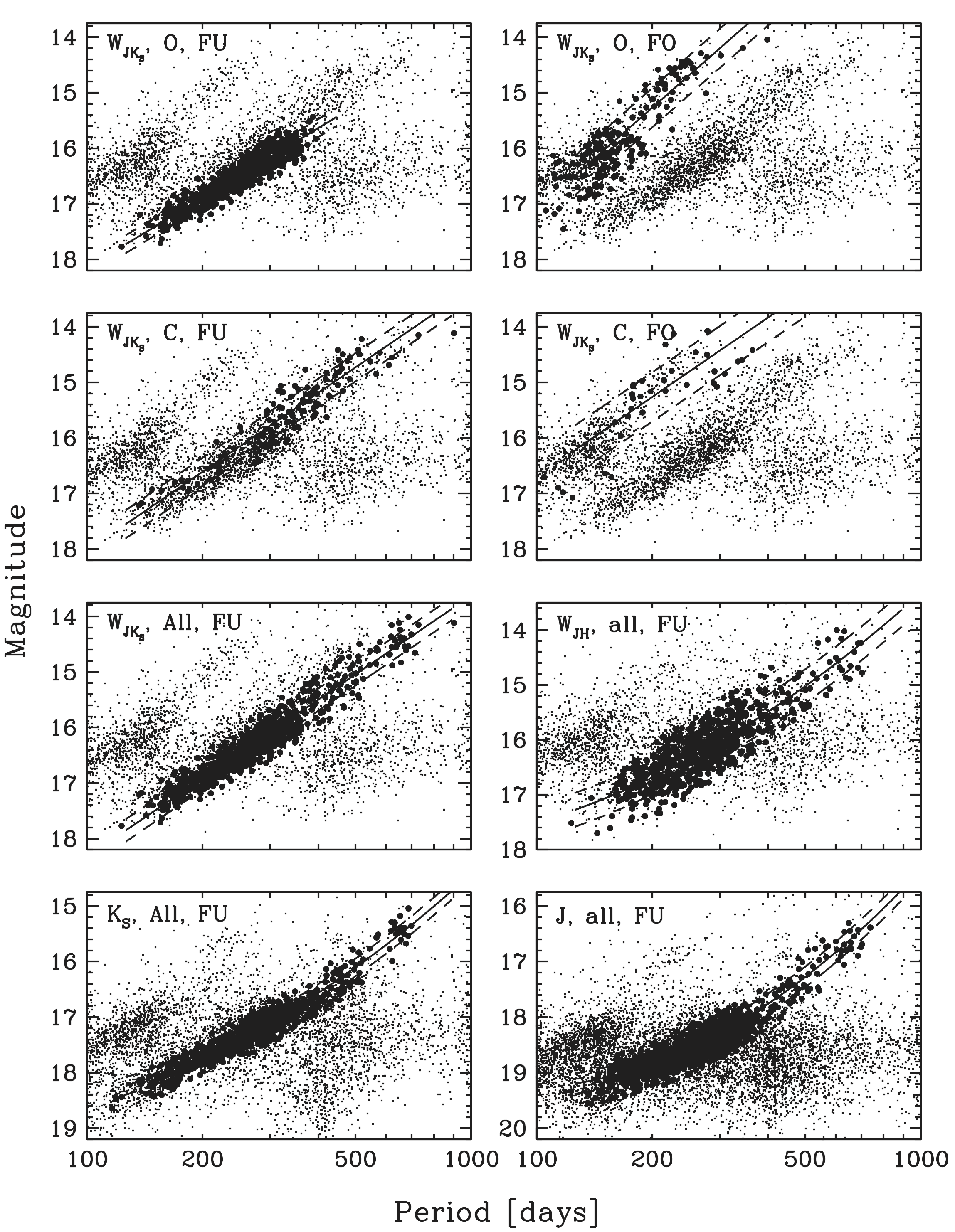
Figure 9: Selected P-L relations (solid lines) and $\pm$1$\sigma$ dispersions for various baseline samples.

4.3 P-L Relations based on OGLE LMC Miras

Sample	Mag	Type	Mode	$a_{0}$	$\sigma(a_{0})$	$a_{1}$	$\sigma(a_{1})$	$a_{2}$	$\sigma(a_{2})$	$N$	$\sigma$	Notes
				[mag]		[mag/dex]		[mag/dex2]			[mag]
Bronze	$W_{JK_{S}}$	O	FU	16.895	0.012	-4.173	0.079	$\dots$	$\dots$	580	0.161	a
Bronze	$W_{JK_{S}}$	O	FO	15.274	0.026	-6.076	0.225	$\dots$	$\dots$	174	0.353
Bronze	$W_{JK_{S}}$	C	FU	16.613	0.049	-4.722	0.181	$\dots$	$\dots$	119	0.253
Bronze	$W_{JK_{S}}$	C	FO	15.267	0.071	-4.743	0.578	$\dots$	$\dots$	36	0.442
Bronze	$W_{JK_{S}}$	All	FU	16.916	0.013	-4.697	0.052	$\dots$	$\dots$	742	0.202
Bronze	$W_{JK_{S}}$	All	FO	15.284	0.024	-5.897	0.206	$\dots$	$\dots$	210	0.372
Bronze	$W_{JH}$	O	FU	16.723	0.023	-3.802	0.143	$\dots$	$\dots$	538	0.287	a
Bronze	$W_{JH}$	O	FO	15.176	0.031	-4.957	0.266	$\dots$	$\dots$	172	0.430
Bronze	$W_{JH}$	C	FU	16.264	0.058	-3.158	0.249	$\dots$	$\dots$	113	0.313
Bronze	$W_{JH}$	C	FO	15.215	0.069	-3.433	0.488	$\dots$	$\dots$	51	0.506
Bronze	$W_{JH}$	All	FU	16.688	0.025	-3.339	0.222	-2.093	0.440	688	0.308
Bronze	$W_{JH}$	All	FO	15.190	0.028	-4.687	0.230	$\dots$	$\dots$	223	0.448
Bronze	$K_{S}$	O	FU	17.711	0.010	-3.670	0.066	$\dots$	$\dots$	592	0.137	a
Bronze	$K_{S}$	O	FO	16.229	0.026	-5.964	0.225	$\dots$	$\dots$	174	0.324
Bronze	$K_{S}$	C	FU	17.559	0.042	-2.579	0.150	$\dots$	$\dots$	122	0.209
Bronze	$K_{S}$	C	FO	16.812	0.062	-3.305	0.467	$\dots$	$\dots$	43	0.386
Bronze	$K_{S}$	All	FU	17.709	0.012	-3.112	0.107	-2.279	0.227	789	0.158
Bronze	$K_{S}$	All	FO	16.323	0.026	-5.287	0.214	$\dots$	$\dots$	211	0.354
Bronze	$H$	O	FU	18.053	0.011	-3.360	0.071	$\dots$	$\dots$	538	0.152	a
Bronze	$H$	O	FO	16.638	0.031	-5.638	0.276	$\dots$	$\dots$	157	0.345
Bronze	$H$	C	FU	17.973	0.038	-1.410	0.164	$\dots$	$\dots$	123	0.251
Bronze	$H$	C	FO	17.395	0.058	-0.895	0.486	$\dots$	$\dots$	59	0.476
Bronze	$H$	All	FU	18.070	0.010	-3.355	0.052	$\dots$	$\dots$	871	0.183
Bronze	$H$	All	FO	16.779	0.028	-4.671	0.256	$\dots$	$\dots$	237	0.369
Bronze	$J$	O	FU	18.821	0.011	-3.094	0.070	$\dots$	$\dots$	783	0.173	a
Bronze	$J$	O	FO	17.455	0.023	-6.084	0.214	$\dots$	$\dots$	234	0.336
Bronze	$J$	C	FU	18.974	0.047	-0.842	0.197	$\dots$	$\dots$	164	0.289
Bronze	$J$	C	FO	18.531	0.091	-4.505	0.519	$\dots$	$\dots$	68	0.621
Bronze	$J$	All	FU	18.839	0.013	-2.493	0.120	-3.565	0.241	1103	0.185
Bronze	$J$	All	FO	17.598	0.022	-5.098	0.169	$\dots$	$\dots$	323	0.366

Table 3: P-L relations for various subsamples. Only baseline fits are shown; see machine-readable version for the full list. a: P$<$400 d.

As a cross-check on the results from §4.2, we carried out a more traditional selection of fundamental-mode Mira candidates by using the LMC dataset previously described in §3.3. We calculated the Wesenheit indices using Eqn. 4 and required a minimum semi-amplitude of $A_{i}\geq 0.5$ mag to match our M33 threshold (equivalent to OGLE’s $\Delta I=1.0$ mag). We note Soszyński et al. (2009) adopted $R^{K_{S}}_{JK_{S}}=0.686$, though one obtains consistent results for relative distance moduli as long as the same $R$ values are adopted for both LMC and M33 samples. We also applied the color-color relations derived in §3.3 to the LMC sample for consistency.

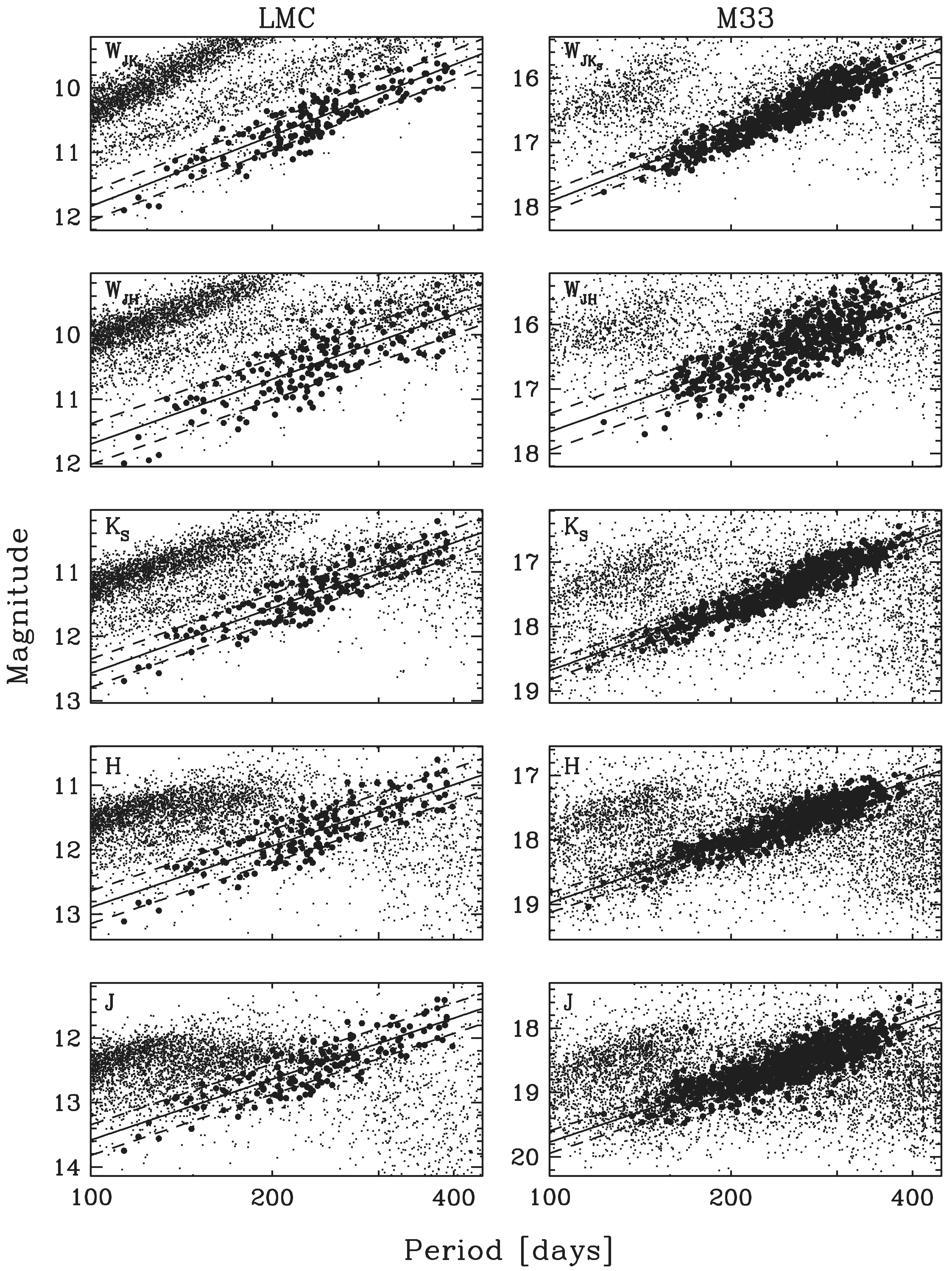
Figure A14: P-L relations for fundamental-mode, O-rich Miras (filled symbols) in the LMC (left) and M33 (right) in various Wesenheit indices and bands. The slopes were determined from the LMC samples and fixed for their M33 counterparts. The solid lines indicate the best-fit relations and the dashed lines indicate the $\pm$1$\sigma$ dispersions.

We fit linear P-L relations following Eq. 5 and applying iterative $2.5\sigma$ clipping to the selected LMC Miras with $P<400$ d. We then solved for the intercept of each corresponding relation for the M33 variables while keeping the slope fixed to the LMC-derived value. The resulting PLRs are shown in Fig. A14, while the PLR coefficients are presented in Table A8. We find good agreement with the PLR zeropoints from Table 3, with differences ranging from $<0.01$ mag to $0.07$ mag.

4.4 Comparison with Yuan et al. (2018)

Yuan et al. (2018) derived PLRs for fundamental-mode O-rich Miras in M33 using the same bands and indices as our study. They also derived periods based on multi-band sinusoidal light curve fits ($IJHK_{S}$, in their case) and separated O- and C-rich Miras using $J-H$ and $H-K_{S}$ color-color relations instead of the procedure we described in §3.3. Their LMC PLRs were based on the same OGLE-III catalog, but they used NIR magnitudes from Yuan et al. (2017b).

We compared the mean magnitudes for Miras in common between our sample and theirs and found good agreement, with mean error-weighted differences (this work $-$ theirs) of $\Delta J=-0.051$, $\Delta H=-0.044$, $\Delta K_{S}=-0.021$, $\Delta W_{JK_{S}}=0.009$ mag and scatter of $\sigma\!\sim$0.2 mag, and $\Delta W_{JH}=-0.044$ mag and scatter of $\sigma\!\sim$0.4 mag, which may be due in part to the different pulsation cycles over which the light curves were sampled by the respective studies.

We applied our selection and fitting procedures to the Mira sample from Table 3 of Yuan et al. (2018), adding our $i$ measurements to carry out the color-color selection described in §3.3 and obtain the most similar comparison possible. We find reasonable agreement with our results, with zeropoints typically within $0.1$ mag of ours and slopes mutually consistent at $<2\sigma$. We note that the PLR based on the $W_{JH}$ index and their magnitudes also exhibits increased scatter relative to the other ones. The fits are provided in Appendix Table A9.

4.5 P-L Relations in gri

Iwanek et al. (2021) analyzed the light curves of LMC Miras at optical and IR wavelengths and derived variability amplitude ratios and phase lags for different bands. They also generated spectral energy distributions (SEDs) based on a high-quality sample of O- and C-rich Miras. These SEDs were used to create synthetic linear PLRs for O- and C-rich Miras in 42 optical and infrared bands, including $gri$.

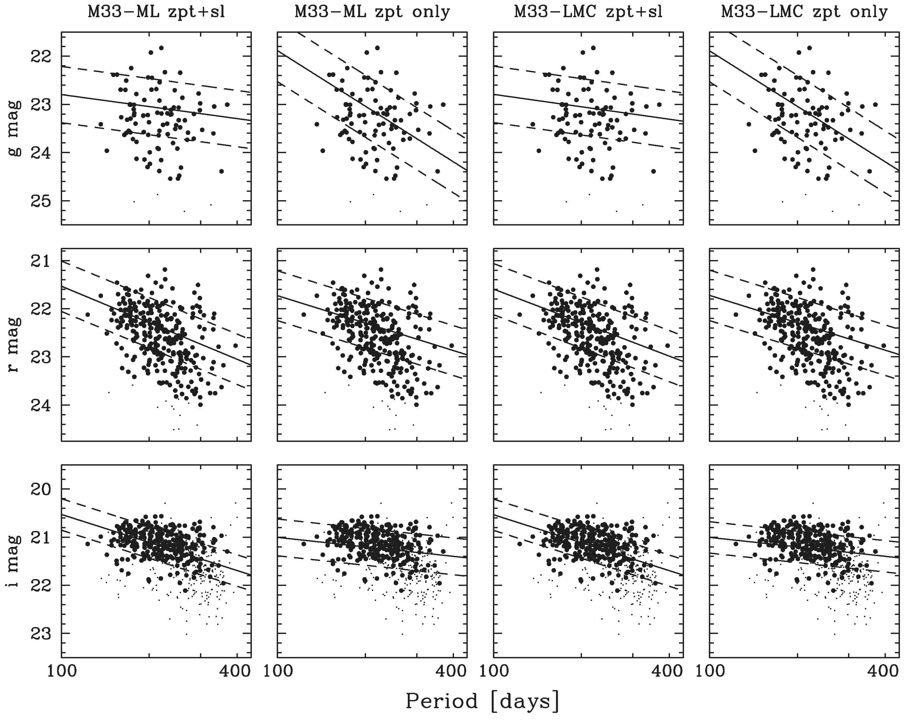
Figure A15: Linear PLRs in $g$ (top), $r$ (middle) and $i$ (bottom) for fundamental-mode O-rich Mira candidates with $P<400$ d identified in §4.1 (M33-ML; left two columns) and §4.3 (M33-LMC; right two columns). For each sample, the left column shows a fit for zeropoint and slope, while the right one fixes the slopes to the values determined by Iwanek et al. (2021).

We fit $gri$ linear PLRs with $2.5\sigma$ clipping in the form of Eq. 5 to the unique O-rich fundamental-mode Mira candidates identified in §4.1 and 4.3 (hereafter referred to as the M33-ML and the M33-LMC samples, respectively). We carried out two sets of fits; one in which we allowed both the intercept and slope to vary and one with slopes fixed to the values from Iwanek et al. (2021). The PLRs are shown in Fig. A15 and the best-fit parameters are listed in Table A10. The intercepts for candidates from the same sample are consistent within their respective uncertainties while the slopes vary significantly. The $i$-band PLR shows the lowest scatter, though it also was fit using more objects than the $g$- and $r$-band ones.

4.6 A Mira-based distance to M33

We estimate a Mira-based distance to M33 using the $W_{JK_{S}}$ PLRs for fundamental-mode O-rich Miras with $P<400$ d from §4.1 and 4.3:

$$\mu_{M33}=a_{0}(M33)-a_{0}(LMC)+\mu_{LMC}$$ (6)

where $\mu_{LMC}$ is the LMC distance modulus based on detached eclipsing binaries from Pietrzyński et al. (2019), $18.477\pm 0.026$ mag, $a_{0}(M33)=16.895\pm 0.012$ mag comes from the first line of Table 3, and $a_{0}(LMC)=10.743\pm 0.020$ mag comes from the first line of Table A8.

We obtain $\mu_{M33}=24.629\pm 0.046$ mag, in good agreement with previous determinations based on a variety of distance indicators (see Breuval et al., 2023, and references therein). The quoted uncertainty is the quadrature sum of the uncertainties listed above, plus an additional 0.03 mag to account for possible systematics in the relative photometric calibration of the LMC and M33 samples.

5 Conclusions

We used multiband observations to identify over 13,000 new Mira candidates and LPVs in M33. We showed that Mira candidates can be robustly identified by using optical light curves and machine-learning techniques, and our measurements in SDSS bands can be used to guide Mira searches in the Rubin/LSST era.

We use near-infrared measurements to further confirm Mira candidates and classify them into various subsamples, detecting for the first time a clear first-overtone pulsation sequence in this galaxy. We also show that NIR observations are very relevant to creating high-fidelity samples of Miras for distance measurements. We use O-rich fundamental-mode Miras with $P<400$ d to determine a distance modulus for M33 of $\mu=24.629\pm 0.046$ mag.

Data Availability

The data underlying this article are available in the article, in its online supplementary material, and on the web at github.com/lmacri/m33sss_miras.

Band	Color	$\chi$	$\xi$	Pivot
		[mag]	[mag/mag]	[mag]
$g$	$g-r$	$-0.078\pm 0.001$	$0.012\pm 0.002$	0.8
	$g-i$	$-0.077\pm 0.001$	$0.006\pm 0.001$	1.5
	$g-z$	$-0.083\pm 0.001$	$0.005\pm 0.001$	1.5
$r$	$g-r$	$-0.010\pm 0.001$	$0.007\pm 0.002$	0.8
	$r-i$	$-0.007\pm 0.001$	$0.026\pm 0.002$	0.8
	$r-z$	$-0.012\pm 0.001$	$0.017\pm 0.002$	1.0
$i$	$g-i$	$-0.155\pm 0.001$	$0.023\pm 0.001$	1.5
	$r-i$	$-0.155\pm 0.001$	$0.051\pm 0.002$	0.8
	$i-z$	$-0.151\pm 0.001$	$0.174\pm 0.007$	0.3
$z$	$g-z$	$0.044\pm 0.001$	$0.011\pm 0.001$	1.5
	$r-z$	$0.041\pm 0.001$	$0.013\pm 0.002$	1.0
	$i-z$	$0.036\pm 0.001$	$-0.012\pm 0.006$	0.3

Table A1: $griz$ photometric transformations.

Band	$\chi$	$\xi$	$\xi^{{}^{\prime}}$
	[mag]	[mag/mag]	[mag/mag2]
$J$	$-0.028\pm 0.001$	$-0.016\pm 0.002$	$-0.035\pm 0.004$
$H$	$-0.043\pm 0.001$	$-0.036\pm 0.003$	$-0.011\pm 0.004$
$K_{S}$	$-0.051\pm 0.002$	$-0.004\pm 0.009$	$\dots$

Table A2: $JHK_{S}$ photometric transformations

Criterion	N
1. Detected in $\geq$1 of $gri$	1,158,951
2. Detected in $i$	1,036,491
3. $J_{i}\geq 0.75$	69,798
4. $r\!-\!i\geq 0$ or no $r$	65,609
5. $R_{i}\geq 0.3$ mag	39,660
6. Detected in $\geq$1 of $JHK_{S}$	14,312

Table A3: Selection of LPVs and Mira candidates.

ID	RA	Dec	$i$	$\sigma_{i}$	$r$	$\sigma_{r}$	$g$	$\sigma_{g}$	$z$	$\sigma_{z}$	$J$	$\sigma_{J}$	$H$	$\sigma_{H}$	$K_{S}$	$\sigma_{K_{S}}$	$J_{i}$	$J_{r}$	$J_{g}$
	[deg]		[mag]		[mag]		[mag]		[mag]		[mag]		[mag]		[mag]
01331383+3036355	23.307608	30.609863	20.530	0.013	22.692	0.024	24.635	0.046	19.773	0.006	17.788	0.007	16.969	0.010	16.531	0.008	4.245	1.342	0.408
01331387+3035040	23.307783	30.584454	21.093	0.004	22.068	0.006	24.002	0.025	20.682	0.011	19.179	0.020	18.375	0.016	17.981	0.011	0.627	-0.014	0.290
01331390+3035156	23.307920	30.587658	20.781	0.003	21.644	0.007	22.744	0.009	20.419	0.018	18.976	0.015	18.133	0.013	17.822	0.010	0.394	0.436	0.463
01331393+3035343	23.308054	30.592873	21.054	0.003	21.587	0.005	22.587	0.005	20.832	0.014	19.359	0.056	18.631	0.019	18.521	0.018	-0.112	0.230	0.026
01331398+3036270	23.308245	30.607506	18.802	0.007	19.745	0.015	21.123	0.007	18.524	0.007	16.819	0.006	16.050	0.004	15.699	0.006	3.553	8.391	1.476
01331400+3036586	23.308348	30.616270	20.356	0.003	21.617	0.006	23.127	0.010	19.904	0.010	18.249	0.011	17.408	0.009	17.070	0.008	0.144	0.501	-0.000
01331401+3036464	23.308376	30.612894	19.221	0.002	19.925	0.004	21.189	0.005	18.915	0.004	17.391	0.006	16.636	0.006	16.329	0.006	0.637	1.796	0.998
01331403+3033509	23.308460	30.564144	21.011	0.009	22.482	0.023	24.311	0.036	20.357	0.007	18.723	0.014	17.800	0.011	17.383	0.010	2.138	1.983	0.336

Table A4: Calibrated photometry of all point sources detected in our analysis. No crowding corrections have been applied.
The full version of this table is available online; only a few representative lines are shown here for guidance.

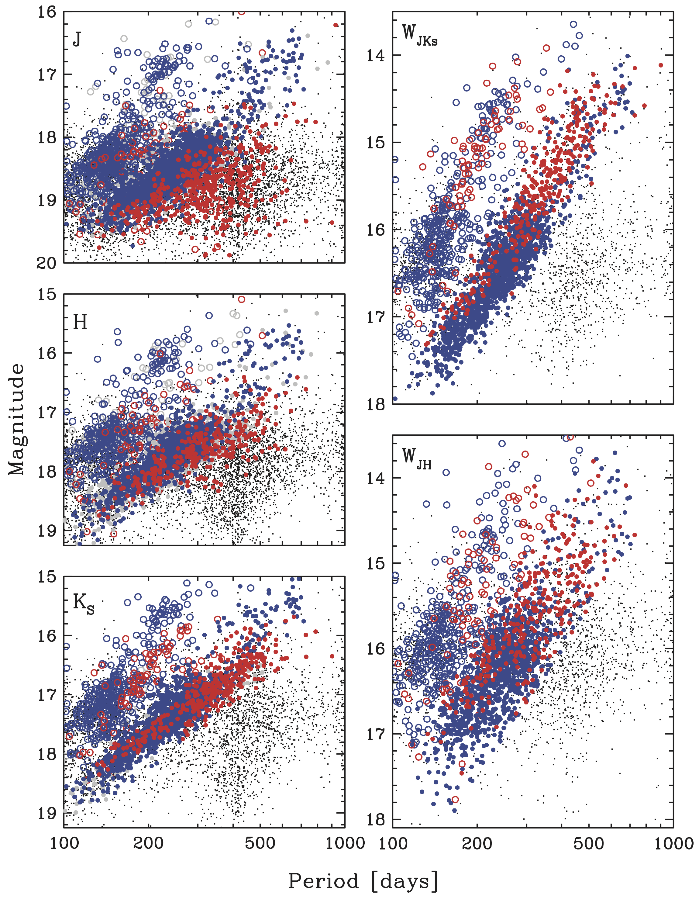
Figure A11: Same as A10, but focusing on the C-rich LPVs.

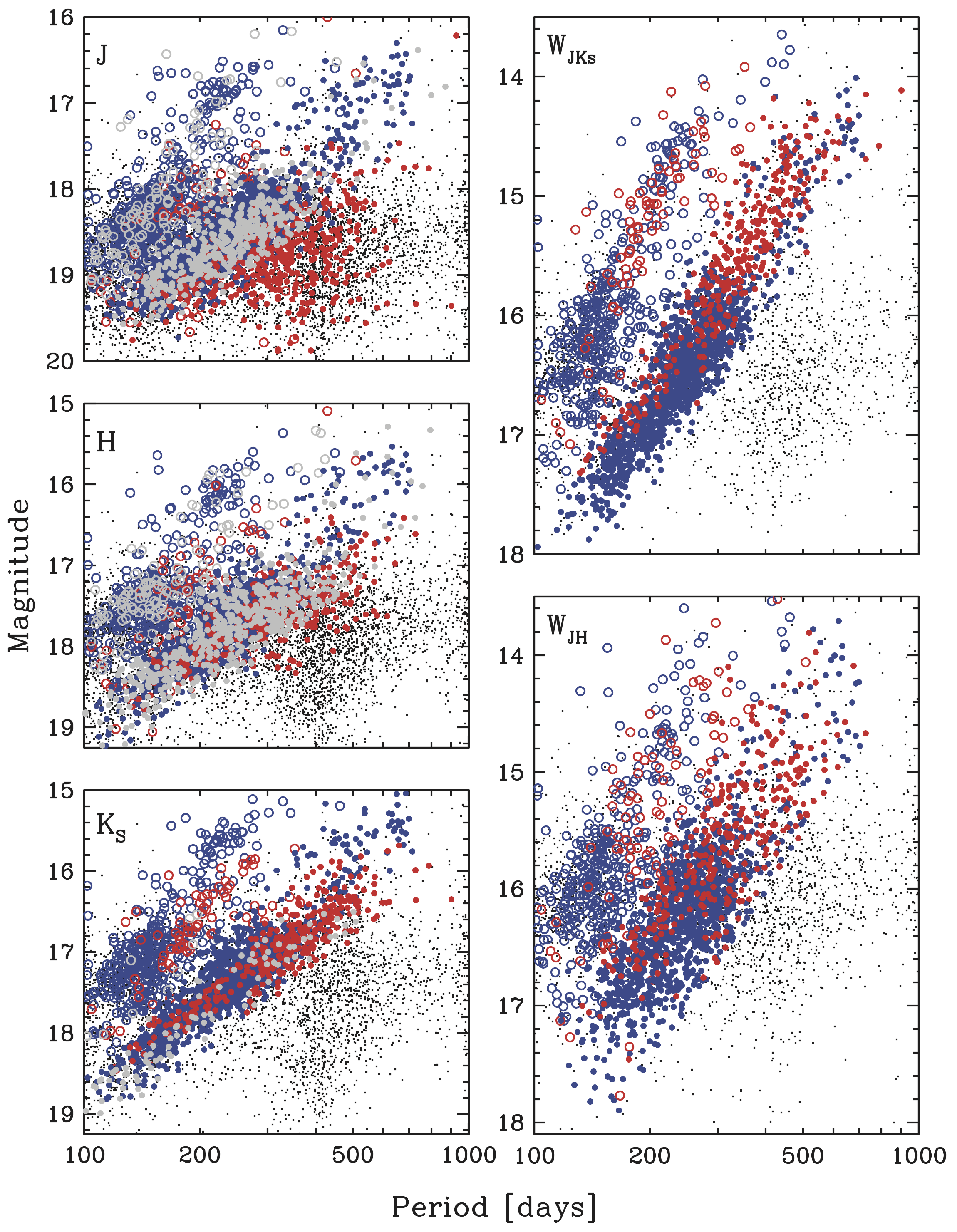
Figure A12: Same as A10, but focusing on the LPVs without O/C classification.

Classifier	Threshold	AUC
Logistic Regression	0.603	0.991
Random Forest	0.195	0.993
Linear Discriminant Analysis	0.758	0.990
Quadratic Discriminant Analysis	0.833	0.991
Kernel SVM	0.845	0.993
Bagging SVM	0.933	0.989

Table A5: Mira/non-Mira thresholds and AUC values for each classifier.

Classifier	Passed	Visual
Logistic Regression	2,335	2,206
Random Forest	2,533	2,404
Linear Discriminant Analysis	2,800	2,637
Quadratic Discriminant Analysis	2,388	2,271
Kernel SVM	2,077	1,989
Bagging SVM	2,511	2,384
Any 1 classifier	3,251	3,052
At least 3 classifiers	2,595	2,454
All 6 classifiers	1,746	1,686

Table A6: Variables passing the threshold for a given classifier, and those remaining after visual inspection, out of a starting sample of 6,144 objects.

ID	RA	Dec	$P$	$i$	$J$	$H$	$K_{S}$	$r$	$g$	$A_{i}$	$A_{J}$	$A_{r}$	$A_{g}$	$\phi_{i}$	$\phi_{J}$	$\sigma_{P}$	$\sigma_{i}$	$\sigma_{J}$	$\sigma_{H}$	$\sigma_{K_{S}}$	$\sigma_{r}$	$\sigma_{g}$	$\sigma_{A_{i}}$	$\sigma_{A_{J}}$	$\sigma_{A_{r}}$
	[deg]		[d]	[mag]						[mag]						[d]	[mag]						[mag]
01322479+3047175	23.103285	30.788191	389.05	20.348	$\dots$	18.074	$\dots$	21.936	23.175	0.766	0.105	0.316	0.326	0.157	0.165	$\dots$	0.004	$\dots$	0.038	$\dots$	0.008	0.005	$\dots$	$\dots$	0.016
01322533+3036126	23.105537	30.603506	1071.52	21.644	$\dots$	17.339	$\dots$	22.958	$\dots$	0.194	0.204	0.266	$\dots$	0.154	0.341	$\dots$	0.008	$\dots$	0.059	$\dots$	0.011	$\dots$	0.012	0.073	$\dots$
01322583+3047503	23.107637	30.797293	1071.52	20.501	$\dots$	18.077	$\dots$	22.071	23.478	0.935	0.142	0.452	0.508	0.023	-0.208	$\dots$	0.004	$\dots$	0.183	$\dots$	0.005	0.007	$\dots$	$\dots$	$\dots$
01322793+3039553	23.116392	30.665359	117.82	21.206	$\dots$	17.756	$\dots$	23.215	$\dots$	0.155	0.092	0.257	$\dots$	0.046	-0.195	$\dots$	0.005	$\dots$	0.023	$\dots$	0.012	$\dots$	$\dots$	$\dots$	0.026
01322879+3049434	23.119947	30.828728	365.78	21.066	$\dots$	17.036	$\dots$	22.939	$\dots$	0.813	0.125	0.453	$\dots$	0.068	0.156	$\dots$	0.004	$\dots$	0.016	$\dots$	0.008	$\dots$	$\dots$	$\dots$	$\dots$
01323222+3041360	23.134270	30.693346	361.46	21.477	$\dots$	17.590	$\dots$	22.586	$\dots$	0.568	0.215	0.777	$\dots$	-0.092	0.167	$\dots$	0.004	$\dots$	0.026	$\dots$	0.013	$\dots$	$\dots$	$\dots$	0.029
01323651+3037358	23.152111	30.626614	161.01	21.957	$\dots$	17.388	$\dots$	$\dots$	$\dots$	0.305	0.027	$\dots$	$\dots$	0.186	-0.181	$\dots$	0.007	$\dots$	0.022	$\dots$	$\dots$	$\dots$	$\dots$	$\dots$	$\dots$
01330333+3038314	23.263865	30.642057	244.74	21.063	20.012	18.492	$\dots$	21.836	$\dots$	0.144	0.082	0.152	$\dots$	0.478	0.500	$\dots$	0.005	0.115	0.074	$\dots$	0.007	$\dots$	$\dots$	$\dots$	0.013
01330346+3041361	23.264431	30.693350	408.17	20.696	17.825	16.674	$\dots$	21.723	$\dots$	0.752	0.498	0.904	$\dots$	0.500	0.184	5.53	0.006	0.037	0.034	$\dots$	0.007	$\dots$	$\dots$	0.035	$\dots$
01330349+3042025	23.264532	30.700701	411.09	20.863	18.972	18.044	$\dots$	$\dots$	23.124	0.358	0.411	$\dots$	1.056	0.200	-0.014	5.92	0.005	0.039	0.030	$\dots$	$\dots$	0.017	$\dots$	$\dots$	$\dots$
01330365+3030497	23.265224	30.513803	395.22	20.232	18.986	$\dots$	$\dots$	20.722	22.154	0.365	0.248	0.494	0.219	0.145	-0.051	$\dots$	0.005	0.052	$\dots$	$\dots$	0.005	0.005	$\dots$	$\dots$	$\dots$
01330549+3038194	23.272890	30.638735	289.39	21.574	18.099	17.620	$\dots$	$\dots$	$\dots$	1.061	0.245	$\dots$	$\dots$	-0.124	0.076	$\dots$	0.005	0.041	0.032	$\dots$	$\dots$	$\dots$	$\dots$	0.050	$\dots$
01330596+3037390	23.274841	30.627512	144.20	21.362	19.027	18.253	$\dots$	22.372	$\dots$	0.311	0.307	0.673	$\dots$	-0.148	-0.279	$\dots$	0.004	0.070	0.074	$\dots$	0.006	$\dots$	$\dots$	$\dots$	$\dots$
01330678+3033068	23.278263	30.551893	448.70	21.978	19.184	$\dots$	17.483	$\dots$	$\dots$	0.263	0.178	$\dots$	$\dots$	-0.117	-0.041	$\dots$	0.006	0.021	$\dots$	0.047	$\dots$	$\dots$	$\dots$	$\dots$	$\dots$
01330706+3034548	23.279436	30.581900	297.75	22.608	18.632	$\dots$	17.336	$\dots$	$\dots$	2.445	0.376	$\dots$	$\dots$	0.206	0.017	$\dots$	0.022	0.026	$\dots$	0.030	$\dots$	$\dots$	0.033	$\dots$	$\dots$
01330740+3032356	23.280830	30.543226	410.86	23.253	$\dots$	$\dots$	18.810	$\dots$	$\dots$	0.520	0.118	$\dots$	$\dots$	-0.360	-0.051	$\dots$	0.019	$\dots$	$\dots$	0.216	$\dots$	$\dots$	0.047	0.314	$\dots$
01330771+3043034	23.282106	30.717609	188.02	21.211	19.661	$\dots$	16.971	22.374	$\dots$	0.352	0.248	0.493	$\dots$	0.471	-0.437	$\dots$	0.007	0.082	$\dots$	0.054	0.005	$\dots$	0.017	0.075	$\dots$
01330991+3035253	23.291283	30.590351	95.80	22.131	19.200	$\dots$	17.895	$\dots$	$\dots$	0.245	0.073	$\dots$	$\dots$	-0.151	-0.128	$\dots$	0.005	0.034	$\dots$	0.111	$\dots$	$\dots$	$\dots$	$\dots$	$\dots$

ID	$\sigma_{A_{g}}$	$\sigma_{\phi_{i}}$	$\sigma_{\phi_{J}}$	Type/	Class	$W_{JK}$	$W_{JH}$	$\sigma_{W_{JK}}$	$\sigma_{W_{JH}}$	MLC scores						MLC threshold						MT	V	Fit(s)
	[mag]			Rej						LR	RAF	LDA	QDA	SVM	BSVM
01322479+3047175	$\dots$	0.001	0.071	RH	FA	$\dots$	$\dots$	$\dots$	$\dots$	$\dots$	$\dots$	$\dots$	$\dots$	$\dots$	$\dots$							0	Z	NA
01322533+3036126	$\dots$	0.007	0.045	LP	FA	$\dots$	$\dots$	$\dots$	$\dots$	$\dots$	$\dots$	$\dots$	$\dots$	$\dots$	$\dots$							0	Z	NA
01322583+3047503	$\dots$	0.001	0.067	CH	FA	$\dots$	$\dots$	$\dots$	$\dots$	$\dots$	$\dots$	$\dots$	$\dots$	$\dots$	$\dots$							0	Z	NA
01322793+3039553	$\dots$	0.006	0.057	ML	FO	$\dots$	$\dots$	$\dots$	$\dots$	0.023	0.000	0.024	0.001	0.001	0.060	0	0	0	0	0	0	0	Z	NA
01322879+3049434	$\dots$	0.001	$\dots$	VZ	FU	$\dots$	$\dots$	$\dots$	$\dots$	0.016	0.278	0.017	0.000	0.688	0.917	0	1	0	0	0	0	1	P	NA
01323222+3041360	$\dots$	0.002	0.009	NU	FU	$\dots$	$\dots$	$\dots$	$\dots$	0.661	0.690	0.640	0.553	0.950	0.986	1	1	0	0	1	1	4	Y	HN qHN
01323651+3037358	$\dots$	0.008	0.099	NO	FO	$\dots$	$\dots$	$\dots$	$\dots$	0.566	0.278	0.827	0.838	0.831	0.968	0	1	1	1	0	1	4	Y	HN qHN
01330333+3038314	$\dots$	0.007	0.171	CJ	FU	$\dots$	$\dots$	$\dots$	$\dots$	$\dots$	$\dots$	$\dots$	$\dots$	$\dots$	$\dots$							0	Z	NA
01330346+3041361	$\dots$	0.001	0.017	CU	FU	$\dots$	14.688	$\dots$	0.112	0.615	0.674	0.623	0.126	0.970	0.998	1	1	0	0	1	1	4	Y	JH lJHN lHN lJN qJH qJHN qHN qJ qJN
01330349+3042025	$\dots$	0.002	0.020	JH	FA	$\dots$	16.442	$\dots$	0.106	$\dots$	$\dots$	$\dots$	$\dots$	$\dots$	$\dots$							0	Z	NA
01330365+3030497	$\dots$	0.001	0.029	RJ	FA	$\dots$	$\dots$	$\dots$	$\dots$	$\dots$	$\dots$	$\dots$	$\dots$	$\dots$	$\dots$							0	Z	NA
01330549+3038194	$\dots$	0.001	0.015	RC	FU	$\dots$	$\dots$	$\dots$	$\dots$	1.000	1.000	1.000	1.000	1.000	1.000	1	1	1	1	1	1	6	M	NA
01330596+3037390	$\dots$	0.001	0.040	OO	FO	$\dots$	16.917	$\dots$	0.234	0.416	0.142	0.581	0.440	0.924	0.977	0	0	0	0	1	1	2	Y	JH lJHN lH lHN lJ lJN qJH qJHN qHN qJ qJN
01330678+3033068	$\dots$	0.004	0.032	JK	FA	16.220	$\dots$	0.084	$\dots$	$\dots$	$\dots$	$\dots$	$\dots$	$\dots$	$\dots$							0	Z	NA
01330706+3034548	$\dots$	0.002	0.021	OU	FU	16.375	$\dots$	0.055	$\dots$	1.000	0.740	1.000	1.000	0.832	0.952	1	1	1	1	0	1	5	Y	JK lJKN lK lKN lJ lJN qJK qJKN qK qKN qJ qJN
01330740+3032356	$\dots$	0.004	0.481	RK	FU	$\dots$	$\dots$	$\dots$	$\dots$	$\dots$	$\dots$	$\dots$	$\dots$	$\dots$	$\dots$							0	Z	NA
01330771+3043034	$\dots$	0.002	$\dots$	CO	FO	14.975	$\dots$	0.112	$\dots$	0.715	0.746	0.909	0.902	0.894	0.980	1	1	1	1	1	1	6	Y	JK lJKN lK lKN lJ qJK qJKN qK qKN qJ
01330991+3035253	$\dots$	0.005	0.071	CK	FO	$\dots$	$\dots$	$\dots$	$\dots$	$\dots$	$\dots$	$\dots$	$\dots$	$\dots$	$\dots$							0	Z	NA

Table A7: Derived properties and associated uncertainties of all LPVs detected in our analysis. All magnitudes are mean values, based on sinusoidal fits. NIR magnitudes have been corrected for crowding. The full version of this table is available online; only a few representative lines are shown here for guidance. Type/Rejection code: CO, Carbon first-overtone; CU, Carbon fundamental-mode; OO, Oxygen first-overtone; OU, Oxygen fundamental-mode; NO, unclassified first-overtone; NU, unclassified fundamental-mode; C[JHK], rejected due to large crowding correction and/or large crowding correction uncertainty in $J$, $H$ or $K_{S}$; RC, rejected due to abnormally blue colors; R[JHK], rejected as faint outliers in $J$, $H$ or $K_{S}$ PLRs; JH/JK, rejected as faint outliers in Wesenheit PLRs; LP, rejected due to best-fit period being at limit of grid search; ML, did not pass any classifier thresholds; VZ, rejected by visual inspection. Class: FU, fundamental mode; FO, first overtone; FA, faint. Machine-learning classifier thresholds: 1, above; 0, below. MT: Sum of MLC thresholds: 6, gold sample; $\geq 3$, silver sample, $\geq 1$, bronze sample. V: Visual inspection: Y, high quality; M, medium quality; N, low quality; Z, rejected before inspection. Fit(s): list of PLRs for which a given variable remained in the final baseline fit after outlier rejection; N/A: not applicable, object rejected before fits.

Host	Mag	$a_{0}$	$\sigma(a_{0})$	$a_{1}$	$\sigma(a_{1})$	$N$	$\sigma$
		[mag]		[mag/dex]			[mag]
LMC	$W_{JK_{S}}$	10.743	0.020	-3.649	0.157	163	0.227
LMC	$W_{JH}$	10.696	0.029	-3.347	0.216	163	0.316
LMC	$K_{S}$	11.560	0.019	-3.368	0.152	163	0.220
LMC	$H$	11.942	0.023	-3.161	0.175	163	0.254
LMC	$J$	12.640	0.022	-3.142	0.162	163	0.237
M33	$W_{JK_{S}}$	16.826	0.007	$\dots$		578	0.166
M33	$W_{JH}$	16.660	0.013	$\dots$		534	0.283
M33	$K_{S}$	17.676	0.006	$\dots$		593	0.140
M33	$H$	18.029	0.006	$\dots$		537	0.151
M33	$J$	18.827	0.006	$\dots$		781	0.173

Table A8: Coefficients of the linear P-L relations fit to O-rich fundamental-mode Miras with $P\!<\!400$ d in the LMC that satisfied the color-color relations from Table 1, and intercepts for the corresponding M33 samples when holding the slopes fixed to the LMC values.

Mag	$a_{0}$	$\sigma(a_{0})$	$a_{1}$	$\sigma(a_{1})$	$N$	$\sigma$
	[mag]		[mag/dex]			[mag]
$W_{JK_{S}}$	16.981	0.008	-4.434	0.054	790	0.177
$W_{JH}$	16.886	0.015	-4.174	0.103	806	0.231
$K_{S}$	17.764	0.004	-3.700	0.026	816	0.184
$H$	18.142	0.004	-3.334	0.027	821	0.199
$J$	18.880	0.004	-3.060	0.028	798	0.209
$W_{JK_{S}}$	16.882	0.007	$\dots$		797	0.195
$W_{JH}$	16.785	0.009	$\dots$		801	0.238
$K_{S}$	17.725	0.006	$\dots$		821	0.192
$H$	18.125	0.006	$\dots$		816	0.197
$J$	18.889	0.007	$\dots$		798	0.208

Table A9: PLRs for O-rich, fundamental-mode Miras in M33 with $125<P<400$ d based on magnitudes from Yuan et al. (2018) and solving for a slope (top set) or holding the slope fixed to the LMC values from Table A8 (bottom set).

Band	Sample	Slope	$a_{0}$	$\sigma(a_{0})$	$a_{1}$	$\sigma(a_{1})$	$N$	$\sigma$
			[mag]		[mag/dex]			[mag]
$g$	M33-ML	Free	23.045	0.058	0.829	0.714	91	0.584
		Fixed	23.033	0.063	3.830	2.378	92	0.645
	M33-LMC	Free	23.049	0.058	0.857	0.702	91	0.585
		Fixed	23.037	0.063	3.830	2.378	92	0.644
$r$	M33-ML	Free	22.289	0.031	2.520	0.354	286	0.523
		Fixed	22.296	0.030	1.892	1.816	300	0.518
	M33-LMC	Free	22.286	0.031	2.311	0.353	283	0.531
		Fixed	22.290	0.030	1.892	1.816	280	0.524
$i$	M33-ML	Free	21.109	0.016	1.936	0.142	531	0.327
		Fixed	21.201	0.015	0.653	1.462	552	0.382
	M33-LMC	Free	21.113	0.016	1.928	0.141	528	0.324
		Fixed	21.201	0.015	0.653	1.462	542	0.369

Table A10: Coefficients associated with the linear $gri$ PLRs fit to the unique, O-rich candidates with $P<400$ d identified using machine learning classifiers (the ML-M33 sample) and the O-rich candidates with $P<400$ d identified by fitting LMC-based PLRs to the M33 Mira candidates (the LMC-M33 sample). The “Slope” columns indicates whether $a_{1}$ was kept fixed or allowed to vary. The $a_{1}$ values and uncertainties for the “Fixed” rows are from Iwanek et al. (2021).

References

- Alcock et al. (1993) Alcock C., et al., 1993, in Soifer B. T., ed., ASP Conf. Ser. Vol. 43, Sky Surveys. Protostars to Protogalaxies. p. 291
- Astropy Collaboration et al. (2013) Astropy Collaboration et al., 2013, A&A, 558, A33
- Boulade et al. (2003) Boulade O., et al., 2003, in Iye M., Moorwood A. F. M., eds, SPIE Conf. Ser. Vol. 4841, Instrument Design and Performance for Optical/Infrared Ground-based Telescopes. pp 72–81, doi:10.1117/12.459890
- Breuval et al. (2023) Breuval L., et al., 2023, ApJ, 951, 118
- Chambers et al. (2016) Chambers K. C., et al., 2016, arXiv, p. arXiv:1612.05560
- Clayton & Feast (1969) Clayton M. L., Feast M. W., 1969, MNRAS, 146, 411
- Cutri et al. (2003) Cutri R. M., et al., 2003, 2MASS All Sky Catalog of point sources. NASA/IPAC
- Glass & Evans (1981) Glass I. S., Evans T. L., 1981, Nature, 291, 303
- Glass & Feast (1982) Glass I. S., Feast M. W., 1982, MNRAS, 199, 245
- Hartman et al. (2006) Hartman J. D., Bersier D., Stanek K. Z., Beaulieu J. P., Kaluzny J., Marquette J. B., Stetson P. B., Schwarzenberg-Czerny A., 2006, MNRAS, 371, 1405
- He et al. (2016) He S., Yuan W., Huang J. Z., Long J., Macri L. M., 2016, AJ, 152, 164
- He et al. (2021) He S., Lin Z., Yuan W., Macri L. M., Huang J. Z., 2021, Annals of Applied Statistics, 15, 662
- Hinkle et al. (2016) Hinkle K. H., Lebzelter T., Straniero O., 2016, ApJ, 825, 38
- Huang et al. (2018) Huang C. D., et al., 2018, ApJ, 857, 67
- Huang et al. (2020) Huang C. D., et al., 2020, ApJ, 889, 5
- Hunter (2007) Hunter J. D., 2007, Computing in Science & Engineering, 9, 90
- Iben & Renzini (1983) Iben I. J., Renzini A., 1983, ARA&A, 21, 271
- Ita et al. (2004) Ita Y., et al., 2004, MNRAS, 347, 720
- Ivezić et al. (2019) Ivezić Ž., et al., 2019, ApJ, 873, 111
- Iwanek et al. (2021) Iwanek P., et al., 2021, ApJS, 257, 23
- Javadi et al. (2015) Javadi A., Saberi M., van Loon J. T., Khosroshahi H., Golabatooni N., Mirtorabi M. T., 2015, MNRAS, 447, 3973
- Jones et al. (2001) Jones E., Oliphant T., Peterson P., et al., 2001, SciPy: Open source scientific tools for Python, scipy.org
- Joye & Mandel (2003) Joye W. A., Mandel E., 2003, in Payne H. E., Jedrzejewski R. I., Hook R. N., eds, ASP Conf. Ser. Vol. 295, ADASS XII. p. 489
- Karakas & Lattanzio (2014) Karakas A. I., Lattanzio J. C., 2014, Publ. Astron. Soc. Australia, 31, e030
- Kato et al. (2007) Kato D., et al., 2007, PASJ, 59, 615
- Kluyver et al. (2016) Kluyver T., et al., 2016, in Loizides F., Schmidt B., eds, Positioning and Power in Academic Publishing: Players, Agents and Agendas. pp 87 – 90
- Kobayashi et al. (2011) Kobayashi C., Karakas A. I., Umeda H., 2011, MNRAS, 414, 3231
- Kukarkin et al. (1958) Kukarkin B. V., Parenago P. P., Efremov Y. I., Kholopov P. N., 1958, General Catalogue of Variable Stars, second edition. Moscow: Academy of Sciences U.S.S.R. Press
- Macri et al. (2001) Macri L. M., Stanek K. Z., Sasselov D. D., Krockenberger M., Kaluzny J., 2001, AJ, 121, 861
- Macri et al. (2015) Macri L. M., Ngeow C.-C., Kanbur S. M., Mahzooni S., Smitka M. T., 2015, AJ, 149, 117
- Madore (1982) Madore B. F., 1982, ApJ, 253, 575
- Markwardt (2009) Markwardt C. B., 2009, in Bohlender D. A., Durand D., Dowler P., eds, ASP Conf. Ser. Vol. 411, ADASS XVIII. p. 251 (arXiv:0902.2850), doi:10.48550/arXiv.0902.2850
- Mattei (1997) Mattei J. A., 1997, Journal of the American Association of Variable Star Observers (JAAVSO), 25, 57
- McClure et al. (1985) McClure R. D., Hesser J. E., Stetson P. B., Stryker L. L., 1985, PASP, 97, 665
- McKinney et al. (2010) McKinney W., et al., 2010, in van der Walt S., Millman J., eds, Vol. 445, Proceedings of the 9th Python in Science Conference. pp 51–56
- Menzies et al. (2019) Menzies J. W., Whitelock P. A., Feast M. W., Matsunaga N., 2019, MNRAS, 483, 5150
- Mink (1999) Mink D. J., 1999, in Mehringer D. M., Plante R. L., Roberts D. A., eds, ASP Conf. Ser. Vol. 172, ADASS VIII. p. 498
- Mordelet & Vert (2014) Mordelet F., Vert J.-P., 2014, Pattern Recognition Letters, 37, 201
- Oliphant (2006) Oliphant T. E., 2006, A guide to NumPy. Vol. 1, Trelgol Publishing USA
- Ou et al. (2023) Ou J.-Y., Ngeow C.-C., Bhardwaj A., Graham M. J., Laher R. R., Masci F. J., Riddle R., 2023, AJ, 165, 137
- Pellerin & Macri (2011) Pellerin A., Macri L. M., 2011, ApJS, 193, 26
- Pietrinferni et al. (2013) Pietrinferni A., Cassisi S., Salaris M., Hidalgo S., 2013, A&A, 558, A46
- Pietrinferni et al. (2021) Pietrinferni A., et al., 2021, ApJ, 908, 102
- Pietrzyński et al. (2019) Pietrzyński G., et al., 2019, Nature, 567, 200
- Planck Collaboration et al. (2020) Planck Collaboration et al., 2020, A&A, 641, A6
- Price-Whelan et al. (2018) Price-Whelan A. M., et al., 2018, AJ, 156, 123
- Puget et al. (2004) Puget P., et al., 2004, in Moorwood A. F. M., Iye M., eds, Vol. 5492, Ground-based Instrumentation for Astronomy. SPIE, pp 978 – 987, doi:10.1117/12.551097
- Riebel et al. (2010) Riebel D., Meixner M., Fraser O., Srinivasan S., Cook K., Vijh U., 2010, ApJ, 723, 1195
- Riess et al. (2019) Riess A. G., Casertano S., Yuan W., Macri L. M., Scolnic D., 2019, ApJ, 876, 85
- Riess et al. (2022) Riess A. G., et al., 2022, ApJ, 934, L7
- Schechter et al. (1993) Schechter P. L., Mateo M., Saha A., 1993, PASP, 105, 1342
- Schlafly & Finkbeiner (2011) Schlafly E. F., Finkbeiner D. P., 2011, ApJ, 737, 103
- Soszyński et al. (2005) Soszyński I., et al., 2005, Acta Astron., 55, 331
- Soszyński et al. (2009) Soszyński I., et al., 2009, Acta Astron., 59, 239
- Soszyński et al. (2013) Soszyński I., Wood P. R., Udalski A., 2013, ApJ, 779, 167
- Stetson (1987) Stetson P. B., 1987, PASP, 99, 191
- Stetson (1994) Stetson P. B., 1994, PASP, 106, 250
- Stetson (1996) Stetson P. B., 1996, PASP, 108, 851
- Tody (1986) Tody D., 1986, in Crawford D. L., ed., SPIE Conf. Ser. Vol. 627, Proc. SPIE. p. 733, doi:10.1117/12.968154
- Udalski et al. (1992) Udalski A., Szymanski M., Kaluzny J., Kubiak M., Mateo M., 1992, Acta Astron., 42, 253
- Whitelock (2013) Whitelock P. A., 2013, in de Grijs R., ed., IAU Symposium Vol. 289, Advancing the Physics of Cosmic Distances. pp 209–216 (arXiv:1210.7307), doi:10.1017/S1743921312021400
- Whitelock & Feast (2000) Whitelock P., Feast M., 2000, Mem. Soc. Astron. Italiana, 71, 601
- Whitelock et al. (1997) Whitelock P. A., Feast M. W., Marang F., Overbeek M. D., 1997, MNRAS, 288, 512
- Whitelock et al. (2008) Whitelock P. A., Feast M. W., Van Leeuwen F., 2008, MNRAS, 386, 313
- Wood & Sebo (1996) Wood P. R., Sebo K. M., 1996, MNRAS, 282, 958
- Yuan (2017) Yuan W., 2017, PhD dissertation, Texas A&M University
- Yuan et al. (2017a) Yuan W., He S., Macri L. M., Long J., Huang J. Z., 2017a, AJ, 153, 170
- Yuan et al. (2017b) Yuan W., Macri L. M., He S., Huang J. Z., Kanbur S. M., Ngeow C.-C., 2017b, AJ, 154, 149
- Yuan et al. (2018) Yuan W., Macri L. M., Javadi A., Lin Z., Huang J. Z., 2018, AJ, 156, 112