Pricing and delta computation in jump-diffusion models with stochastic intensity by Malliavin calculus

Abstract: In this paper, the pricing of financial derivatives and the calculation of their delta Greek are investigated as the underlying asset is a jump-diffusion process in which the stochastic intensity component follows the CIR process. Utilizing Malliavin derivatives for pricing financial derivatives and challenging to find the Malliavin weight for accurately calculating delta will be established in such models. Due to the dependence of asset price on the information of the intensity process, conditional expectation attribute to show boundedness of moments of Malliavin weights and the underlying asset is essential. Our approach is validated through numerical experiments, highlighting its effectiveness and potential for risk management and hedging strategies in markets characterized by jump and stochastic intensity dynamics.

keywords:Malliavin calculus, stochastic intensity, delta computing, pricing of derivatives, Bismuth-Elworthy-Li formula.

1 Introduction

Stochastic intensity is the most important attribute of financial markets which represent the realism of the arrival rate of events in the models better. Flexibility in randomness of intensity, in spite of constant intensity, can remarkably capture the arrival of new information, changes in the behavior of investors in the market and the arrival rate of jumps such as market crashes, large price movements, or sudden changes in volatility. Financial institutions, portfolio managers, and investors can use these models to assess the likelihood and potential consequences of extreme events, leading to more informed decision-making and the development of effective risk mitigation strategies, see [Brigo and Alfonsi(2005)] and [Leung and Kwok(2009)] respectively. In addition, the stochastic jump intensity to the rate of default of firms for risk assessments and portfolio managements have been exposed in [Feng(2017)] and [Lévy dit Véhel and Lévy Véhel(2018)].
The self-exciting point process in which the current intensity of events is determined by events in the past is firstly introduced by [Hawkes(1971)]. The crucial role of jumps with stochastic intensity in option pricing are supported by the empirical results in [Fang(2000)] and its role in modeling the jump intensity risk is supported in [Santa-Clara and Yan(2010)], empirically. In Markov intensity models with discrete state, which the model called Markov-modulated jump model, pricing of the risky underlying assets is considered by [Elliott et al.(2007)], [Bo et al.(2010)], [Chang et al.(2013)] and recently by [Shan et al.(2023)] in which the Markov-modulated jump diffusion process is used to model the discrete dividend process in financial markets. In the continuous framework, [Brigo and Alfonsi(2005)] have derived an analytical formula for pricing of credit derivatives under CIR stochastic intensity models. Later, [Brigo and El-Bachir(2006)] have considered a smile-extended jump stochastic intensity to price credit default swaptions. Non-Gaussian intensity models have been investigated by [Bianchi and Fabozzi(2015)]. In 2019, the authors [Yang et al.(2019)] proposed these models for variance exchange rate to price the variance swaps. This subject in [Huang et al.(2014)] and in [Chang and Wang(2020)] and recently in [Ma et al.(2023)] was dealt with option pricing under double exponential jump model with stochastic volatility and stochastic intensity using Fourier transform.
On the other hand, Malliavin calculus is a sophisticated mathematical tool that extends the traditional calculus to differentiate random variables and quantify their sensitivities, the accurate calculation of delta and pricing of financial derivatives, hedging strategies, and investment decision-making, see for instance, [Alos and Ewald(2008)], [Hillairet et al.(2018)], [Yilmaz(2018)], [Kuchuk-Iatsenko et al.(2016)], [Fournié et al.(2001)]. In 2004, [El-Khatib and Privault(2004)] have computed Greeks in a market driven by a discontinuous process with Poisson jump times and random jump sizes using the Malliavin calculus on Poisson space. Numerical simulations are presented for the delta and gamma of Asian options, and confirm the efficiency of this approach over classical finite difference Monte-Carlo approximations of derivative. In [Huehne(2005)] the stochastic weights for the fast and accurate computation of Greeks for options whose underlying is driven by a pure-jump Levy process have been derived. Later, Bavouset and Messaoud discuss this subject [Bavouzet and Messaoud(2006)] by both the Malliavin derivative with respect to the jump amplitudes and to the Wiener process. Also, The computation of delta with Malliavin calculus for options on the underlying asset modeled by Levy processes are stated in [Mhlanga(2011)], [Khedher(2012)], [Matchie(2009)], [Coffie et al.(2021)], as we refer the readers to [Nunno et al.(2009)], [Nualart and Nualart(2018)] for more details about the Malliavin calculus on Levy processes. Recently, sensitivity analysis with respect to the stock price for singular SDEs is considered in [Coffie et al.(2021)] and regularity of distribution-dependent SDEs with jump processes is proved in [Song and Wang(2022)] by using Malliavin calculus. [Hudde and Rüschendorf(2023)] have represented a closed-form expression for Asian Greeks in an exponential Levy process model.
In general, in this article, we are interested in the jump-diffusion models with stochastic intensity as follows in the CIR model, called self-exciting Cox process. We will investigate the pricing of financial derivatives and will derive an expression for the delta calculation by a Malliavin weight. In the presence of the Malliavin derivative of the intensity in the Malliavin derivative of the underlying process, some Wiener-direction which belongs to the domain of Skorokhod operator in the Gaussian case is found, Theorem 3.3, to be used in the duality formula appeared in calculating the delta and the price of financial derivatives. Meanwhile, the use of conditional expectation with respect to the information of the intensity is unavoidable. We should point out here that there are two different approaches to define the Malliavin derivative with respect to jump processes {chapters 10, 11 of [Nualart and Nualart(2018)]}. So that we will find two different Skorokhod integrals as the Malliavin weight associated to each approach in computation of delta.
This article is organized as follows: In section 2, we recall Malliavin concepts on Wiener spaces and Poisson spaces. In section 3, we will introduce the main model with a stochastic intensity process and check the necessities to exist the solution of the model and to be bounded of its moments, We will demonstrate the Malliavin derivative of the solution and find some direction which its derivative is invertible in. In section 4, we will calculate the delta and price of the European option . In section 5, We express the numerical results and compare them with the finite difference method. Finally, we introduce the fund that supported us and we present the conclusion.

2 A review on Malliavin calculus

Let us review some concepts of Malliavin calculus on Wiener space and in the Poisson framework, See standard reference [Nualart and Nualart(2018)].

2.1 Malliavin calculus concepts on Wiener space

For a positive real number $T$, suppose that $\Omega:=C_{0}(\left[0,T\right])$ is the space of real continuous functions $w$ on $\left[0,T\right]$ with $w(0)=0$ equipped with the uniform norm

$$\rVert{w}\rVert_{\infty}=\sup_{t\in\left[0,T\right]}\lvert{w(t)}\rvert.$$ (2.1)

Consider $\Big{(}\Omega,\mathcal{F},\mathcal{F}_{t},P\Big{)}$ as a filtered probability space, with coordinate map $t\to{W(t,w)}$ for Brownian motion $B(t)$ corresponding to the filtration $\{\mathcal{F}_{t}\}$. For every $\gamma\in\Omega$ of the Cameron-Martin space, the set of the functions in the form $\gamma(t)=\int_{0}^{t}g(s)ds$ for some $g\in{L^{2}}(\left[0,T\right])$, and a random variable $F:\Omega\to{\mathbb{R}}$, the directional derivative of $F$ in the $\gamma$ direction, have defined as the following form, if the limit exists. In fact,

$$D^{W}_{\gamma}{F}(w)=\frac{d}{d\epsilon}[F(w+\epsilon\gamma)]_{\epsilon=0}.$$

If there exists some $\psi\in{L^{2}(\left[0,T\right]\times\Omega)}$ satisfying the following equation

$$D^{W}_{\gamma}{F}(w)=\int_{0}^{T}\psi(t,w).g(t)dt.$$

the variable $F$ is Malliavin differentiable in Wiener space and $D^{W}F=(D^{W}_{t}{F})_{0\leq{t}\leq{T}}:=(\psi(t,w))_{0\leq{t}\leq{T}}$. We define the set of all $F:\Omega\to\mathbb{R}$ such that $F$ is differentiable by $\mathbb{D}_{W}^{1,2}$. In fact, if we denote by $\mathcal{S}$ the set of all functionals $F=\varphi(\theta_{1},\theta_{2},...,\theta_{n})$ where $\phi$ is a smooth function with bounded derivatives of any order and $\theta_{i}=\int_{0}^{T}f_{i}(t)dB_{t}$ with $f_{i}\in{L^{2}(\left[0,T\right])}$, Then $F\in\mathbb{D}_{W}^{1,2}$ and the derivative of $F$ is

$$D^{W}_{t}{F}(w)=\sum_{i=1}^{n}\frac{\partial{\varphi}}{\partial x_{i}}(\theta_{1},....,\theta_{n})f_{i}(t).$$

For every integer $n$ and $p\geq 2$, the space $\mathbb{D}_{W}^{n,p}$ is the closure of $\mathcal{S}$ with respect to the norm defined by

$$\lVert{F}\rVert_{n,p}=\lVert{F}\rVert_{L^{p}(\Omega)}+\lVert{(D^{W})^{n}{F}}\rVert_{L^{p}(\left[0,T\right]^{n}\times\Omega)}.$$

The Skorohod operator is the adjoint operator of $D_{W}$ from $L^{2}([0,T]\times\Omega)$ to $\mathbb{D}_{W}^{1,2}$. Later, we will use the following duality relation, which states that for given $F\in\mathbb{D}^{1,2}$ and $u\in Dom(\delta^{W})$

$$\mathbb{E}\Big{(}\left\langle{D^{W}F,u}\right\rangle_{L^{2}[0,T]}\Big{)}:=\mathbb{E}\Big{(}\int_{0}^{T}(D^{W}_{t}F)u_{t}dt\Big{)}=\mathbb{E}\Big{(}F\delta^{W}(u)\Big{)}.$$

For every adapted process $u$, $\delta^{W}(u)$ can be represented by the stochastic integral $\int_{0}^{T}u(s)dW_{s}$.

2.2 The Malliavin calculus on Poisson space

There are two different approach to introduce the Malliavin derivative of Levy processes. One is introduced by the chaos expansion criteria which does not satisfy in the rule chain, and the other is introduced on the closure of the set of Poisson functionals that satisfies the chain rule. We recall some concepts and for more details, we refer to [Nualart and Nualart(2018)].

2.2.1 First approach

Consider a Levy process $N$ with the Levy measure $v$ on a complete separable metric space $(\mathbb{R}_{0},\mathcal{B})$. Let $L^{2}([0,T]\times\mathbb{R}_{0}^{n})$ be the space of symmetric square integrable functions on the $([0,T]\times\mathbb{R}_{0}^{n},m\times v\times\cdots\times v)$, where $m$ is an atomless measure on $[0,T]$. Given $h\in L^{2}([0,T]\times\mathbb{R}_{0}^{n})$ and fixed $z\in\mathbb{R}_{0}$, we write $h(t,.,z)$ to indicate the function on $\mathbb{R}_{0}^{n-1}$ given by $(z_{1},...,z_{n-1})\to h(t,z_{1},...,z_{n-1},z)$. Denote the set of random variables $F$ in $L^{2}(\Omega)$ with a chaotic decomposition $F=\sum_{n=0}^{\infty}I_{n}(h_{n})$ by $\mathbb{D}_{N}^{1,2}$, that $h_{n}\in L_{s}^{2}([0,T]\times\mathbb{R}_{0}^{n})$, satisfying

$$\sum_{n\geq 1}nn!\lVert{h_{n}}\rVert_{L^{2}([0,T]\times\mathbb{R}_{0}^{n})}^{2}<\infty.$$

Then, if $F\in\mathbb{D}_{N}^{1,2}$ we define the Malliavin derivative $D^{N}$ of $F$ as the $L^{2}([0,T]\times\mathbb{R}_{0})$-valued random variable given by

$$D_{t,z}^{N}F=\sum_{n\geq 1}nI_{n-1}(h_{n}(t,.,z)),\;\;z\in\mathbb{R}_{0}.$$

The operator $D^{N}$ is a closed operator from $\mathbb{D}_{N}^{1,2}\subset L^{2}(\Omega)$ into $L^{2}(\Omega\times[0,T]\times\mathbb{R}_{0})$ and satisfy the following rules.

Lemma 2.1.

[Nualart and Nualart(2018)] Let $F,G\in\mathbb{D}_{N}^{1,2}$ Suppose that $FG\in L^{2}(\Omega)$ and $(F+D^{N}F)(G+D^{N}G)\in L^{2}(\Omega\times[0,T]\times\mathbb{R}_{0})$.Then the product FG also belongs to $\mathbb{D}_{N}^{1,2}$ and

$$D_{t,z}^{N}(FG)=FD_{t,z}^{N}G+GD_{t,z}^{N}F+D_{t,z}^{N}FD_{t,z}^{N}G.$$

proposition 2.2.

[Nualart and Nualart(2018)] Let $F$ be a random variable in $\mathbb{D}^{1,2}$ and let $\varphi$ be a real continuous function such that $\varphi(F)$ belongs to $L^{2}(\Omega)$ and $\varphi(F+D^{N}F)$ belongs to $L^{2}(\Omega\times Z)$. Then $\varphi(F)$ belongs to $\mathbb{D}^{1,2}$ and

$$D_{t,z}^{N}\varphi(F)=\varphi(F+D_{t,z}^{N}F)-\varphi(F).$$

Now, given stochastic process $u$ in $L^{2}(\Omega\times[0,T]\times\mathbb{R}_{0})$ admits a unique representation of the following form that for each $(t,z)\in[0,T]\times\mathbb{R}_{0}$

$$u(t,z)=\sum_{n\geq 0}I_{n}(h_{n}(t,.,z)),$$

where the function $h_{n}\in L^{2}([0,T]\times\mathbb{R}_{0}^{n})$. If

$$\sum_{n\geq 0}(n+1)!\lVert{h_{n}}\rVert_{L(\mathbb{R}_{0}^{n+1})}^{2}<\infty,$$

we say $u$ is in the domain of the divergence operator $\delta^{N}$, denoted by $Dom\delta^{N}$ and

$$\delta^{N}(u)=\sum_{n\geq 0}I_{n+1}(\tilde{h}_{n}),$$

where $\tilde{h}_{n}$ stands for the symmetrization of $h$ as a function in the last $n+1$ variables. For instance, if $u(z)=h(z)$ is a deterministic function in $L^{2}(\mathbb{R}_{0})$ then $\delta(u)=I_{1}(h)$. If $u(z)=I_{1}(h(.,z))$, with $h\in L^{2}(\mathbb{R}_{0})$, then $\delta(u)=I_{2}(h)$.
The following result characterizes $\delta^{N}$ as the adjoint operator of $D^{N}$.

proposition 2.3.

[Nualart and Nualart(2018)] If $u\in Dom\delta^{N}$, then $\delta^{N}(u)$ is the unique element of $L^{2}(\Omega)$ such that, for all $F\in\mathbb{D}_{N}^{1,2}$,

$$\mathbb{E}(\left\langle{D^{N}F,u}\right\rangle_{L^{2}([0,T]\times\mathbb{R}_{0})})=\mathbb{E}(F\delta^{N}(u)).$$

Conversely, if $u$ is a stochastic process in $L^{2}(\Omega\times[0,T]\times\mathbb{R}_{0})$ such that, for some $G\in L^{2}(\Omega)$ and for all $F\in\mathbb{D}_{N}^{1,2}$,

$$\mathbb{E}(\left\langle{D^{N}F,u}\right\rangle_{L^{2}([0,T]\times\mathbb{R}_{0})})=\mathbb{E}(FG),$$

then $u$ belongs to $Dom\delta^{N}$ and $\delta^{N}(u)=G$.

The divergence operator $\delta$ satisfies the following product rule.

proposition 2.4.

[Nualart and Nualart(2018)] Let $F\in\mathbb{D}_{N}^{1,2}$ and $u\in Dom\delta$ such that the product $uDF$ belongs to $Dom\delta^{N}$ and the right-hand side of (2.2) below belongs to $L^{2}(\Omega)$. Then $Fu\in Dom\delta$ and

$$\delta^{N}(Fu)=F\delta^{N}(u)-\left\langle{D^{N}F,u}\right\rangle_{L^{2}([0,T]\times\mathbb{R}_{0})}-\delta^{N}(uDF).$$ (2.2)

2.2.2 Second approach

We make use of the notation

$$N(h):=\int_{[0,T]}\int_{\mathbb{R}_{0}}h(t,z)N(dt.dz)$$

for every $h\in L^{1}([0,T]\times\mathbb{R}_{0},m\times v)$. Denote by $C_{0}^{0,2}([0,T]\times\mathbb{R}_{0})$ the set of continuous functions $h:[0,T]\times\mathbb{R}_{0}\to\mathbb{R}$ that have compact support and are twice differentiable on $\mathbb{R}_{0}$. We consider the set $\mathcal{S}$ of cylindrical random variables of the form

$$F=\varphi(N(h_{1}),...,N(h_{n})),$$ (2.3)

where $\varphi\in C_{0}^{2}(\mathbb{R}^{n})$ and $h_{i}\in C_{0}^{0,2}([0,T]\times\mathbb{R}_{0})$ for $1\leq i\leq n$. It is easy to show that the set $\mathcal{S}$ is dense in $L^{2}(\Omega)$. The Malliavin derivative of a simple random variable $F$ in $\mathcal{S}$ of the form (2.3) is defined as the two parameter process

$$D_{t,z}^{N_{P}}F=\sum_{k=1}^{n}\frac{\partial\varphi}{\partial x_{k}}(N(h_{1}),...,N(h_{n}))\partial_{z}h_{k}(t,z),\;\quad(t,z)\in[0,T]\times\mathbb{R}_{0}.$$

In particular, $D_{t,z}^{N_{P}}(N(h))=\partial_{z}h$. Define the scalar product $<.,.>$ for every $u,\tilde{u}\in L^{2}(\Omega)$ as

$$<u,\tilde{u}>_{N}:=\int_{0}^{T}\int_{\mathbb{R}_{0}}u(s,z)\tilde{u}(s,z)N(ds,dz),$$

and denote $\|.\|_{N}$ as its associated norm. Also, let $\mathbb{D}_{N_{p}}^{1,p}$, for every $p\geq 1$, the closure of $\mathcal{S}$, as the domain of the operator $D_{t,z}^{N_{P}}$, with respect to the seminorm

$$\|F\|_{1,N}^{p}:=\mathbb{E}(|F|^{p})+\mathbb{E}(\|D^{N_{P}}F\|^{p}_{N}).$$

The next result is the chain rule for the Malliavin derivative in the Poisson framework.

proposition 2.5.

[Nualart and Nualart(2018)] Let $\varphi$ be a function in $C^{1}(\mathbb{R})$ with bounded derivative, and let $F$ be a random variable in $\mathbb{D}_{N_{p}}^{1,2}$. Then, $\varphi(F)$ belongs to $\mathbb{D}_{N_{p}}^{1,2}$ and

$$D_{t,z}^{N_{P}}(\varphi(F))=\varphi^{\prime}(F)D_{t,z}^{N_{P}}(F).$$

The authors in [Song and Wang(2022)] have stated a powerful tool called integration by parts formula for this type of derivative in the following form in some Sobolev spaces we recall here. For every $p\geq 1$, denote by $\mathbb{L}_{p}$ the set of all predictable processes $\psi$ on $[0,T]\times\mathbb{R}_{0}$ with finite norm

$$\|\psi\|_{\mathbb{L}_{p}}=\Big{[}\mathbb{E}\Big{(}\int_{\mathbb{R}_{0}}\int_{0}^{T}\psi(s,z)m(ds)\nu(dz)\Big{)}^{p}\Big{]}^{\frac{1}{p}}+\Big{[}\mathbb{E}\Big{(}\int_{\mathbb{R}_{0}}\int_{0}^{T}\psi^{p}(s,z)m(ds)\nu(dz)\Big{)}\Big{]}^{\frac{1}{p}},$$

and denote by $\mathbb{V}_{p}$ the set of all predictable processes $\psi$ on $[0,T]\times\mathbb{R}_{0}$ with finite norm

$$\|\psi\|_{\mathbb{V}_{p}}=\|\frac{\partial\psi}{\partial z}\|_{\mathbb{L}_{p}}+\|\rho\psi\|_{\mathbb{L}_{p}},$$

where $\rho(z)=|z|^{-1}$. We shall write $\mathbb{V}_{\infty}:=\bigcap_{p\geq 1}\mathbb{V}_{p}$.

proposition 2.6.

Given $F\in\mathbb{D}_{N_{p}}^{1,p}$, for $p\geq 2$, and $w_{0}\in\mathbb{V}_{\infty}$ we have

$$\mathbb{E}\Big{(}<D^{N_{P}}(F),w_{0}>_{N}\Big{)}=\mathbb{E}\Big{(}F\int_{\mathbb{R}_{0}}\int_{0}^{T}\frac{1}{\theta}\frac{\partial(\theta w_{0})}{\partial z}(t,z)\tilde{N}(dt,dz)\Big{)},$$

where $\nu(dz)=\theta(z)dz$.

3 Stochastic jump processes with stochastic intensity

In this section, we recall the concept of stochastic intensity desired by Bérmaud in Chapter 5 of [Brèmaud(2020)] and introduce the model and state the assumptions and some lemmas we need in the main results.
Let $(\Omega,\mathcal{F},\mathit{P})$ be a Wiener-Poisson space with a risk neutral probability $\mathit{P}$. Assume that $N_{t}$ is a Poisson process and $\mathcal{F}_{t}^{N}$ is an $\sigma$-field generated by $N$ with the density of jumps sizes $C_{z}$, as $z\in\mathbb{R}_{0}$ and stochastic intensity process $\lambda$. For given $\sigma$-field $\mathcal{F}_{t}$, the process $\lambda_{t}$ is an $\mathcal{F}_{t}$-intensity of $N_{t}$ if for every $s,t\in[0,T]$

$$\mathbb{E}\Big{(}\int_{\mathbb{R}_{0}}\int_{t}^{s}N(du,dz)|\mathcal{F}_{t}\Big{)}=\mathbb{E}\Big{(}\int_{\mathbb{R}_{0}}\int_{t}^{s}C_{z}\lambda_{u}dudz|\mathcal{F}_{t}\Big{)},$$

and so that $\tilde{N}(t,z)=N(t.z)-\int_{\mathbb{R}_{0}}\int_{0}^{t}C_{z}\lambda_{s}dsdz$ is an $\mathcal{F}_{t}$-martingale. Also, obviously, for every $0\leq t,s\leq T$ and for every $\mathcal{F}_{t}$-predictable function $k$

$$\mathbb{E}\Big{(}\int_{\mathbb{R}_{0}}\int_{t}^{s}k(u,z)N(du,dz)|\mathcal{F}_{t}\Big{)}=\mathbb{E}\Big{(}\int_{\mathbb{R}_{0}}\int_{t}^{s}k(u,z)C_{z}\lambda_{u}dudz|\mathcal{F}_{t}\Big{)}.$$

We refer the reader to Chapter 5 of [Brèmaud(2020)] for more details. It is worth mention that one can easily show [Brèmaud(2020)] that if $\lambda$ is $\mathcal{G}$-measurable, for every measurable function $k$ such that $\mathbb{E}\Big{(}\int_{\mathbb{R}_{0}}\int_{0}^{t}(k(t,s))^{2}\lambda_{s}dsC_{z}dz\Big{)}<\infty$,

$$\mathbb{E}\Big{(}exp\{iu\int_{\mathbb{R}_{0}}\int_{0}^{t}k(s,z)N(ds,dz)\}\Big{|}\mathcal{G}\Big{)}=exp\Big{\{}\int_{\mathbb{R}_{0}}\int_{0}^{t}(e^{iuk(t,z)}-1)\lambda_{s}C_{z}dsdz\Big{\}}.$$ (3.1)

In this manuscript, we assume that the underlying asset price $S=(S_{t})_{t\in[0,T]}$ with the jump stochastic intensity process $\lambda=(\lambda_{t})_{t\in[0,T]}$ of Poisson process $N_{t}$ can be governed by the following system of SDEs:

$$\begin{cases}dS_{t}&=\mu S_{t}dt+\sigma_{1}S_{t}dW_{t}^{S}+\int_{\mathbb{R}_{0}}(e^{J_{t,z}}-1)S_{t}\tilde{N}(dt,dz),\\ d\lambda_{t}&=\kappa(\Theta-\lambda_{t})dt+\sigma_{2}\sqrt{\lambda_{t}}dW_{t},\end{cases}$$ (3.2)

where $(W_{t})_{t\in[0,T]}$ and $(W_{t}^{S})_{t\in[0,T]}$ are independent Brownian motions, $N_{t}$ is independent of $W_{t}^{S}$, $\mu$ denotes the riskless interest rate, $J$ is a cadlag function, the mean-reverting speed parameter $\kappa,\sigma_{2}$ and $\sigma_{1}$ are positive constants and the long term mean $\Theta$ satisfying $2\kappa\Theta\;>\sigma_{2}^{2}$.
For $\mathcal{F}_{t}^{\lambda}$, $\sigma$-field generated by $\lambda$, let $\mathcal{F}_{t}=\mathcal{F}_{t}^{N}\vee\mathcal{F}_{t}^{\lambda}$ and $\mathcal{G}=\mathcal{F}_{t}^{\lambda}$. In this case, obviously, $\mathcal{F}_{t}=\mathcal{F}_{t}^{N}$ and for every $0\leq t,s\leq T$ and for every $\mathcal{F}_{t}$-predictable function $k$

$$\mathbb{E}\Big{(}\int_{\mathbb{R}_{0}}\int_{t}^{s}k(u,z)N(du,dz)|\mathcal{F}_{t}^{\lambda}\Big{)}=\int_{\mathbb{R}_{0}}\int_{t}^{s}k(u,z)C_{z}\lambda_{u}dudz.$$

We also assume the following conditions throughout the paper.
Condition H1:

• For every $p\geq 1$ and for almost everywhere $0\leq t\leq T$

  $$\int_{\mathbb{R}_{0}}(e^{J_{t,z}}-1)^{p}C_{z}dz\leq u_{p}<\infty,\qquad v_{t}:=\int_{\mathbb{R}_{0}}(e^{J_{t,z}}-1)C_{z}dz\neq 0.$$ (3.3)

• There exists some $p_{0}\geq 2$ such that $2u_{p_{0}}\sigma_{2}^{2}\leq k$.

• $\int_{0}^{T}\frac{1}{v_{u}^{2}}du<\infty.$

we know that the solution to the stochastic differential (3.2) is as follows, see [Øksendal and Sulem(2019)].

$$S_{t} =S_{0}\exp\Big{\{}(\mu-\frac{\sigma_{1}^{2}}{2})t+\sigma_{1}W_{t}^{S}+\int_{0}^{t}\int_{\mathbb{R}_{0}}(J_{s,z}-e^{J_{s,z}}+1)C_{z}\lambda_{s}dzds$$

$$+\int_{\mathbb{R}_{0}}\int_{0}^{t}J_{s,z}\tilde{N}(ds,dz)\Big{\}}$$

$$=:S_{0}\exp\Big{\{}X_{t}\Big{\}}=:S_{0}Y_{t}\exp\Big{\{}(\mu-\frac{\sigma_{1}^{2}}{2})t+\sigma_{1}W_{t}^{S}\Big{\}},$$

where $Y_{t}$ satisfying

$$dY_{t}=Y_{t}(e^{J_{t,z}}-1)\tilde{N}(dt,dz),\qquad Y_{0}=1.$$ (3.4)

It follows that this solution is in $L^{p}$-space for every $2\leq p\leq p_{0}$, as we see in the following lemma.

Lemma 3.1.

The solution $S_{t}$ of (3.2) is unique and uniformly is in $\bigcap_{2\leq p\leq p_{0}}L^{p}(\Omega)$, i.e., for every $2\leq p\leq p_{0}$,

$$\mathbb{E}\Big{(}\sup_{0\leq t\leq T}|S_{t}|^{p}\Big{)}<\infty.$$

Proof.

We know that for any $p\geq 2$,

$$\mathbb{E}\Big{(}\sup_{t\in\left[0,T\right]}\exp\Big{\{}p(\mu-\frac{\sigma_{1}^{2}}{2})t+p\sigma_{1}W_{t}^{S}\Big{\}})<\infty.$$

So, it is sufficient to show that equation (3.4) has a unique solution. To do this, with the same proof of Lemma 2.3. in [Song and Zhang(2015)] and Section 5.1.1 of [Menaldi(2008)], we derive that for any $p\geq 2$ and every step time $h$, there exists a constant $C_{p}>0$ such that:

$$\mathbb{E}\biggl{(}\sup_{s\in\left[t,t+h\right]}\bigg{|}\int_{\mathbb{R}_{0}}\int_{t}^{s} (e^{J_{u,z}}-1)Y_{u}\tilde{N}(du,dz)\bigg{|}^{p}|\mathcal{F}_{t}^{\lambda}\biggr{)}$$

$$\leq{C_{p}}\mathbb{E}\biggl{(}\bigg{[}\int_{t}^{t+h}\int_{\mathbb{R}_{0}}Y_{u}^{2}(e^{J_{u,z}}-1)^{2}C_{z}\lambda_{u}dzdu\bigg{]}^{\frac{p}{2}}|\mathcal{F}_{t}^{\lambda}\biggr{)}$$

$$+{C_{p}}\mathbb{E}\biggl{(}\bigg{[}\int_{t}^{t+h}\int_{\mathbb{R}_{0}}Y_{u}^{p}(e^{J_{u,z}}-1)^{p}C_{z}\lambda_{u}dzdu|\mathcal{F}_{t}^{\lambda}\biggr{)}.$$

Define the new probability measure $p_{1}(A)=\lambda_{s}1_{A}(s)/\int_{t}^{t+h}\lambda_{s}ds$, for every $A\subset[t,t+h]$ as $1_{A}$ is the indicator function, and applying Young inequality to result

$$\mathbb{E}\biggl{(}\sup_{s\in\left[t,t+h\right]}Y_{s}^{p}|\mathcal{F}_{t}^{\lambda}\biggl{)} \leq\mathbb{E}\big{(}Y_{t}^{p}|\mathcal{F}_{t}^{\lambda}\big{)}$$

$$+{C_{p}}\frac{1}{\int_{t}^{t+h}\lambda_{s}ds}\mathbb{E}\biggl{(}\bigg{[}\int_{t}^{t+h}\int_{\mathbb{R}_{0}}Y_{u}^{p}(e^{J_{u,z}}-1)^{p}C_{z}\lambda_{u}dzdu|\mathcal{F}_{t}^{\lambda}\biggr{)}$$

$$+{C_{p}}\mathbb{E}\biggl{(}\bigg{[}\int_{t}^{t+h}\int_{\mathbb{R}_{0}}Y_{u}^{p}(e^{J_{u,z}}-1)^{p}C_{z}\lambda_{u}dzdu|\mathcal{F}_{t}^{\lambda}\biggr{)}$$

$$\leq\mathbb{E}\big{(}Y_{t}^{p}|\mathcal{F}_{t}^{\lambda}\big{)}+{C_{p}}\frac{u_{p}}{\int_{t}^{t+h}\lambda_{s}ds}\int_{t}^{t+h}\mathbb{E}\biggl{(}\sup_{t\leq s\leq u}Y_{s}^{p}|\mathcal{F}_{t}^{\lambda}\biggr{)}\lambda_{u}du$$

$$+{C_{p}}u_{p}\int_{t}^{t+h}\mathbb{E}\biggl{(}\sup_{t\leq s\leq u}Y_{s}^{p}|\mathcal{F}_{t}^{\lambda}\biggr{)}\lambda_{u}du.$$ (3.5)

Now apply Gronwall inequality for $m(s)=\int_{t}^{s}\mathbb{E}\big{(}\sup_{t\leq s\leq u}Y_{s}^{p}|\mathcal{F}_{t}^{\lambda}\big{)}\lambda_{u}du$, $0\leq s\leq T$, and derive that

$$m(s) \leq\mathbb{E}\big{(}Y_{t}^{p}|\mathcal{F}_{t}^{\lambda}\big{)}\int_{t}^{s}\lambda_{u}exp\Big{\{}u_{p}\int_{u}^{s}\lambda_{r}(1+\frac{1}{\int_{t}^{s}\lambda_{v}dv})dr\Big{\}}du$$

$$\leq\mathbb{E}\big{(}Y_{t}^{p}|\mathcal{F}_{t}^{\lambda}\big{)}e^{u_{p}}\int_{t}^{s}\lambda_{u}exp\Big{\{}u_{p}\int_{u}^{s}\lambda_{r}dr\Big{\}}du$$

$$\leq\mathbb{E}\big{(}Y_{t}^{p}|\mathcal{F}_{t}^{\lambda}\big{)}\frac{e^{u_{p}}}{u_{p}}exp\Big{\{}u_{p}\int_{t}^{s}\lambda_{r}dr\Big{\}}.$$ (3.6)

Substituting (3.6) into (3.5) obtain

$$\mathbb{E}\biggl{(}\sup_{s\in\left[t,t+h\right]}Y_{s}^{p}|\mathcal{F}_{t}^{\lambda}\biggl{)}\leq\mathbb{E}\big{(}Y_{t}^{p}|\mathcal{F}_{t}^{\lambda}\big{)}\biggl{(}1+C_{p}(1+\frac{1}{\int_{t}^{t+h}\lambda_{s}ds})exp\Big{\{}u_{p}+u_{p}\int_{t}^{s}\lambda_{r}dr\Big{\}})\biggr{)}.$$ (3.7)

Therefore, in the sequence, we should show that the expectation of the right hand side of equation (3.6), as $t=0$ and $2\leq p\leq p_{0}$, is bounded. For this purpose, we note that using Ito formula, for a positive constant $\gamma$, we have

$$de^{\gamma\lambda_{t}} =\gamma\kappa(\Theta-\lambda_{t})e^{\gamma\lambda_{t}}+\sigma_{2}\gamma e^{\gamma\lambda_{t}}\sqrt{\lambda_{t}}dW_{t}+\frac{\sigma_{2}^{2}}{2}\gamma^{2}e^{\gamma\lambda_{t}}\lambda_{t}dt$$

$$=\kappa\Theta\gamma e^{\gamma\lambda_{t}}dt+(\frac{\gamma^{2}\sigma_{2}^{2}}{2}-\kappa\gamma)\lambda_{t}e^{\gamma\lambda_{t}}dt+\sigma_{2}\gamma e^{\gamma\lambda_{t}}\sqrt{\lambda_{t}}dW_{t}.$$

Taking the expectation on both sides and applying Gronwall inequality to deduce

$$\mathbb{E}(e^{\gamma\lambda_{t}})\leq e^{\gamma\lambda_{0}}+\kappa\Theta\gamma e^{\gamma\lambda_{0}}e^{\kappa\Theta\gamma t}=e^{\gamma\lambda_{0}}(1+\kappa\Theta\gamma e^{\kappa\Theta\gamma t}),$$

Now, set $\gamma=u_{p_{0}}$ and $\gamma=2u_{p_{0}}$ in above inequality to use in the expectation of the following equation.

$$\int_{0}^{t}\kappa\Theta\gamma e^{\gamma\lambda_{s}}ds=e^{\gamma\lambda_{t}}-e^{\gamma\lambda_{0}}+\int_{0}^{t}\kappa\gamma\lambda_{s}e^{\gamma\lambda_{s}}ds-\frac{\gamma^{2}\sigma_{2}^{2}}{2}\int_{0}^{t}\lambda_{s}e^{\gamma\lambda_{s}}ds-\gamma\sigma_{2}\int_{0}^{t}\sqrt{\lambda_{s}}e^{\gamma\lambda_{s}}dW_{s}.$$

Thus,

$$\kappa\Theta\gamma\mathbb{E}\big{(}\int_{0}^{t}e^{\gamma\lambda_{s}}ds\big{)} \leq\mathbb{E}(e^{\gamma\lambda_{t}})-e^{\gamma\lambda_{0}}+\kappa\gamma\mathbb{E}\big{(}\int_{0}^{t}\lambda_{s}e^{\gamma\lambda_{s}}ds\big{)}$$

$$\leq\mathbb{E}(e^{\gamma\lambda_{t}})-e^{\gamma\lambda_{0}}+\kappa\gamma\int_{0}^{t}[2\mathbb{E}(\lambda_{s}^{2})+2\mathbb{E}(e^{2\gamma\lambda_{s}})]ds<\infty,$$

which results that

$$\mathbb{E}\big{(}exp\{u_{p_{0}}\int_{0}^{t}\lambda_{s}ds\}\big{)}\leq\int_{0}^{t}\mathbb{E}(exp\{u_{p_{0}}\lambda_{s}\})ds<\infty.$$

This fact and taking the expectation from (3.7) complete the proof. The inequality (3.7) will obviously prove the uniqueness of the solution. ∎

remark 3.2.

We mention that if $sup_{p\geq 2}u_{p}<\infty$, then Lemma 3.1 is held for every $p\geq 2$.

In the last part of this section note that getting the partial derivatives of $S_{t}$ with respect to $S_{0}$ show that the stochastic flow of $S_{t}$ exists and it is

$$\frac{\partial{S_{t}}}{\partial{S_{0}}}=\frac{S_{t}}{S_{0}}=\exp\{X_{t}\}=Y_{t}\exp\{(\mu-\frac{\sigma_{1}^{2}}{2})t+\sigma_{1}W_{t}\}.$$ (3.8)

Therefore, this flow is in $L^{p}$-space for every $2\leq p\leq p_{0}$.

3.1 Malliavin derivative of the solution on Wiener space

In this section, we obtain Malliavin derivative of the solution $S_{t}$ and also we will consider some Skorokhod integrable directions in which the inverse of directional derivatives are in $L^{p}(\Omega)$, for all $2\leq p\leq p_{0}$.
Due to the representation of the solution with respect to $X_{t}$, it needs to find its derivative. Gaussian Malliavin derivative of $X_{t}$ comes as follows:

$$D_{u}^{W}X_{t}=-\int_{u}^{t}D_{u}^{W}\lambda_{s}\int_{\mathbb{R}_{0}}(e^{J_{s,z}}-1)C_{z}dzds=:-\int_{u}^{t}v_{u}D_{u}^{W}\lambda_{s}ds,$$ (3.9)

In [Altmayer and Neuenkirch(2015)], the authors have shown that using the Ito formula and taking the Malliavin derivative with respect to the Brownian motion, for every $s\leq t$

$$D_{s}^{W}\lambda_{t}=\sigma_{2}\sqrt{\lambda_{t}}1_{0\leq s\leq t}\exp\Big{\{}-{\int_{s}^{t}(\frac{\kappa}{2}+\frac{C_{\sigma}}{\lambda_{r}})dr}\Big{\}},$$ (3.10)

$$\mathbb{E}(\sup_{0\leq t\leq T}\lambda_{t}^{p})<\infty\quad\forall p\geq 1,\quad and\quad\sup_{0\leq t\leq T}\mathbb{E}(\lambda_{t}^{-p})<\infty,\quad\forall p\geq 1~{}s.t.~{}2\kappa\theta>p\sigma_{2}^{2},$$ (3.11)

where $C_{\sigma}=\frac{\kappa\Theta}{2}-\frac{\sigma_{2}^{2}}{8}$ is a positive number. Here, we represent that the inverse of directed Malliavin derivative of $X_{t}$ in some directions, which are also in the domain of Skorokhod operator, can belong to all $L^{p}$ spaces for any $p\geq 2$.

Theorem 3.3.

When $2\kappa\theta>3\sigma_{2}^{2}$, there exists a direction $h(.)\in dom(\delta^{W})$, defined as the following

$$h(u)=\frac{1}{v_{u}}(\frac{\kappa}{2}+\frac{C_{\sigma}}{\lambda_{u}}),\qquad 0\leq u\leq T,$$

such that $\mathcal{B}_{T}=\left\langle{D_{.}^{W}X_{T},h(.)}\right\rangle$ is almost surely invertible and

$$\Big{(}\left\langle D_{.}^{W}X_{T},h(.)\right\rangle\Big{)}^{-1}\in\bigcap_{2\leq p}L^{p}.$$

Proof.

From (3.9), Fubini theorem and the expression (3.10), we derive

$$\mathcal{B}_{T} =-\int_{0}^{T}\left\langle v_{.}{D_{.}^{W}\lambda_{s},h(.)}\right\rangle ds$$

$$=-\int_{0}^{T}\Big{[}\sigma_{2}\sqrt{\lambda_{s}}exp\{-\int_{0}^{s}(\frac{\kappa}{2}+\frac{C_{\sigma}}{\lambda_{r}})dr\}\int_{0}^{s}(\frac{\kappa}{2}+\frac{C_{\sigma}}{\lambda_{u}})exp\{\int_{0}^{u}(\frac{\kappa}{2}+\frac{C_{\sigma}}{\lambda_{r}})dr\}du\Big{]}ds$$

$$=-\int_{0}^{T}\Big{[}\sigma_{2}\sqrt{\lambda_{s}}(1-exp\{-\int_{0}^{s}(\frac{\kappa}{2}+\frac{C_{\sigma}}{\lambda_{r}})dr\})\Big{]}ds.$$ (3.12)

Applying the Gamma function results

$$\mathbb{E}(\frac{1}{|\mathcal{B}_{T}|^{p}})= \frac{1}{\Gamma(p)}\mathbb{E}\big{(}\int_{0}^{\infty}z^{p-1}e^{-z\int_{0}^{T}\Big{[}\sigma_{2}\sqrt{\lambda_{s}}(1-exp\{-\int_{0}^{s}(\frac{\kappa}{2}+\frac{C_{\sigma}}{\lambda_{r}})dr\})\Big{]}ds}dz\big{)}$$

$$\leq\frac{1}{\Gamma(p)}\mathbb{E}\big{(}\int_{0}^{\infty}z^{p-1}e^{-z(1-e^{-\frac{T\kappa}{2}})\int_{0}^{T}\sigma_{2}\sqrt{\lambda_{s}}ds}dz\big{)}$$

$$=\frac{1}{\sigma_{2}^{p}(1-e^{-\frac{T\kappa}{2}})^{p}}\mathbb{E}\big{(}\frac{1}{(\int_{0}^{T}\sqrt{\lambda_{s}}ds)^{p}}\big{)}<\infty,$$

thanks to Lemma 5.2. of [Altmayer and Neuenkirch(2015)] in the last inequality. So, we conclude that for every $p\geq 2$, $\mathcal{B}_{T}\in L^{P}(\Omega)$. In the sequel, we will show that $h(.)\in Dom(\delta^{W})$. According to Proposition 1.3.1 in [Nualart(2000)], it is sufficient to show that $h(.)\in\mathbb{D}_{W}^{1,2}$. To do that, from these facts that for every $x,y\in\mathbb{R}$, $(x+y)^{2}\leq 2x^{2}+2y^{2}$ we result

$$\mathbb{E}(\int_{0}^{T} h^{2}(t)dt)+\mathbb{E}(\int_{0}^{T}(D^{W}h)^{2}(t)dt)$$

$$\leq\kappa^{2}\int_{0}^{T}\frac{1}{2v_{u}^{2}}du+2C_{\sigma}^{2}\int_{0}^{T}\frac{1}{v_{u}^{2}}\mathbb{E}(\frac{1}{\lambda_{u}^{2}})du+\sigma_{2}^{2}C_{\sigma}^{2}\int_{0}^{T}\frac{1}{v_{u}^{2}}\mathbb{E}(\frac{1}{\lambda_{u}^{3}})du<\infty,$$ (3.13)

where we used form (3.11) in the last inequality. ∎

4 Pricing and Delta calculation

In this section, we discuss the pricing of the payoff function by weighted Malliavin described in the previous section.we also present an explicit formula to calculate the delta Greek. To do this, we state a representation of the delta as a combination of the Wiener-Malliavin weight and the Poisson-Malliavin weight. We assume the following condition on the payoff functions.
Condition H2: The payoff function $\mathit{f}:\mathbb{R^{+}}\to\mathbb{R^{+}}$ is a measurable function with at most polynomial growth $\frac{p_{0}}{2}$, and locally Riemann integrable, possibly, having discontinuities of the first kind.
Let us introduce the following notations presented in [Bezborodov et al.(2019)]: for every $x\geq 0$,

$$F(x)=\int_{0}^{x}\mathit{f}(z)dz,\qquad\mathit{g(y)}=\mathit{f(e^{y})},\qquad G(y)=\int_{0}^{y}\mathit{g}(z)dz.$$

In this notation, we have $\mathbb{E}\mathit{f}(S_{T})=\mathbb{E}\mathit{g}(X_{T})$ and

$$G(x)=\frac{F(e^{x})}{e^{x}}+\int_{0}^{x}\frac{F(e^{y})}{e^{y}}dy-F(1).$$

Theorem 4.1.

Under condition H2, the price of a simple derivative can be represented as

$$\mathbb{E}\Big{(}\mathit{f}(S_{T})\Big{)}=\mathbb{E}\Big{(}\frac{F(S_{T})}{S_{T}}(1+{Z_{T}})\Big{)}=\mathbb{E}\Big{(}G(X_{T})Z_{T}\Big{)},$$ (4.1)

where $Z_{T}=\delta^{W}(\frac{h(.)}{\mathcal{B}_{T}})$.

Proof.

Suppose that the function $\mathcal{K}$ is a locally Lipschitz function with $\mathcal{K}^{\prime}(x)=k(x)$ almost everywhere with respect to the Lebesgue measure. Assume additionally that $k$ is of exponential growth and $\mathcal{K}(X_{T})\in\mathbb{D}_{W}^{1,2}$. Namely, the Skorokhod integral is the adjoint operator to the Malliavin derivative, therefore

$$\mathbb{E}\Big{(}k(X_{T})\Big{)} =\mathbb{E}\Big{(}\int_{0}^{T}k(X_{T})\frac{D_{u}^{W}X_{T}h(u)}{\left\langle{D_{.}^{W}X_{T},h(.)}\right\rangle}du\Big{)}$$

$$=\mathbb{E}\Big{(}\int_{0}^{T}\frac{D_{u}^{W}\mathcal{K}(X_{T})h(u)}{\left\langle{D_{.}^{W}X_{T},h(.)}\right\rangle}du\Big{)}=\frac{1}{T}\mathbb{E}\Big{(}\int_{0}^{T}\mathcal{K}(X_{T})\frac{h(.)}{\left\langle{D_{.}^{W}X_{T},h(.)}\right\rangle}dW_{u}\Big{)}$$

$$=\mathbb{E}\Big{(}\mathcal{K}(X_{T})\int_{0}^{T}\frac{h(u)}{\left\langle{D_{.}^{W}X_{T},h(.)}\right\rangle}dW_{u}\Big{)}=\mathbb{E}\Big{(}\mathcal{K}(X_{T})Z_{T}\Big{)}.$$ (4.2)

In particular, for the function $G$ which is a locally Lipschitz function and $g$ is of exponential growth, we rewrite (4.1) for $k=g$ as follows:

$$\mathbb{E}(f(S_{T})) =\mathbb{E}(g(X_{T}))=\mathbb{E}(G(X_{T})Z_{T})$$

$$=\mathbb{E}\Big{(}\Big{(}\frac{F(S_{T})}{S_{T}}+\int_{0}^{X_{T}}\frac{F(e^{y})}{e^{y}}dy-F(1)\Big{)}Z_{T}\Big{)}$$

$$=\mathbb{E}\Big{(}\frac{F(S_{T})}{S_{T}}Z_{T}\Big{)}+\mathbb{E}\Big{(}Z_{T}\int_{0}^{X_{T}}\frac{F(e^{y})}{e^{y}}dy\Big{)}-\mathbb{E}\Big{(}F(1)Z_{T}\Big{)}$$

$$=\mathbb{E}\Big{(}\frac{F(S_{T})}{S_{T}}Z_{T}\Big{)}+\mathbb{E}\Big{(}\int_{0}^{X_{T}}\frac{F(e^{y})}{e^{y}}dyZ_{T}\Big{)},$$

Applying equation (4.1) to $k(x)=\frac{F(e^{x})}{e^{x}}$, we get that

$$\mathbb{E}\Big{(}\int_{0}^{X_{T}}\frac{F(e^{y})}{e^{y}}dyZ_{T}\Big{)}=\mathbb{E}\Big{(}\frac{F(e^{X_{T}})}{e^{X_{T}}}\Big{)}=\mathbb{E}\Big{(}\frac{F(S_{T})}{S_{T}}\Big{)}.$$

Hence

$$\mathbb{E}\Big{(}f(S_{T})\Big{)}=\mathbb{E}\Big{(}\frac{F(S_{T})}{S_{T}}Z_{T}\Big{)}+\mathbb{E}\Big{(}\frac{F(S_{T})}{S_{T}}\Big{)}=\mathbb{E}\Big{(}\frac{F(S_{T})}{S_{T}}(1+{Z_{T}})\Big{)}.$$

∎

4.0.1 Delta with Wiener-Malliavin weight

Now, we are ready to present an explicit formula to calculate the Delta Greek. To do this, we state a representation of the delta as a combination of the Wiener-Malliavin weight and the Poisson-Malliavin weight.

Theorem 4.2.

Under condition H2, the delta display with respect to the Wiener -Malliavin weight as

$$\Delta^{W}= \frac{\partial}{\partial{s}}\mathbb{E}\Big{(}f(S_{T})\Big{)}=\mathbb{E}\Big{(}f(S_{T})\frac{Z_{T}}{S_{0}}\Big{)}.$$

Proof.

From the fact that $\frac{\partial{Z_{T}}}{\partial{S_{0}}}=0$, we derive

$$\Delta^{W} =\frac{\partial}{\partial{S_{0}}}\mathbb{E}\Big{(}f(S_{T})\Big{)}=\frac{\partial}{\partial{S_{0}}}\mathbb{E}\Big{(}\frac{F(S_{T})}{S_{T}}(1+{Z_{T}})\Big{)}$$

$$=\mathbb{E}\Big{(}\frac{\frac{\partial{F(S_{T})}}{\partial{S_{0}}}S_{T}-F(S_{T})\frac{\partial{S_{T}}}{\partial{S_{0}}}}{S_{T}^{2}}(1+{Z_{T}})+\frac{F(S_{T})}{S_{T}}\frac{\partial{Z_{T}}}{\partial{S_{0}}}\Big{)}$$

$$=\mathbb{E}\Big{(}(\frac{F^{\prime}(S_{T})}{S_{T}}-\frac{F(S_{T})}{{S_{T}}^{2}})\frac{\partial{S_{T}}}{\partial{S_{0}}}(1+{Z_{T}})\Big{)}$$

$$=\mathbb{E}\Big{(}\frac{f(S_{T})}{S_{T}}\frac{{S_{T}}}{{S_{0}}}(1+{Z_{T}})\Big{)}-\mathbb{E}\Big{(}\frac{F(S_{T})}{{S_{T}}^{2}}\frac{{S_{T}}}{{S_{0}}}(1+{Z_{T}})\Big{)}$$

$$=\mathbb{E}\Big{(}\frac{f(S_{T})}{S_{0}}(1+{Z_{T}})\Big{)}-\mathbb{E}\Big{(}\frac{F(S_{T})}{S_{T}}\frac{1}{{S_{0}}}(1+{Z_{T}})\Big{)}$$

$$=\mathbb{E}\Big{(}\frac{f(S_{T})}{S_{0}}{Z_{T}}\Big{)},$$

where we used Theorem 4.1 in the last equality. ∎

4.0.2 Delta with Poisson-Malliavin weight

We will use the literature in [Coffie et al.(2021)] and calculate the delta with a Malliavin weight regarding the Poisson random measure in two approaches.
In the first approach.
Due to Proposition 2.2, we know that $D_{u,z}^{N}X_{t}=J_{u,z}1_{u\leq t}$ and then $D_{u,z}^{N}S_{t}=S_{t}(exp\{D_{u,z}^{N}X_{t}\}-1)$ satisfying

$$D_{s,z}^{{N}}S_{t} =S_{s}(e^{J_{s,z}}-1)+\int_{s}^{t}\mu D_{s,z}^{N}S_{u}du+\int_{s}^{t}\sigma_{1}D_{s,z}^{N}S_{u}dW_{u}$$

$$+\int_{s}^{t}\int_{\mathbb{R}_{0}}(e^{J_{u,z}}-1)D_{s,z}^{N}S_{u}\tilde{N}(du,dz).$$ (4.3)

It is remarkable that in this approach of Malliavin derivative with respect ot the Poisson random measure, the following lemma will be held.

Lemma 4.3.

Let $F=1_{A}\in\mathbb{D}_{N}^{1,2}$, where $1_{A}$ is the indicator function of the set $A\in\mathcal{F}$. Then $D^{N}F=0$ almost everywhere.

Proof.

From Proposition 2.2 and Lemma 2.1, we have

$$D^{N}1_{A} =D^{N}(1_{A})^{2}=(1_{A}+D^{N}1_{A})^{2}-1_{A}^{2}=21_{A}D^{N}1_{A}+(D^{N}1_{A})^{2},$$

$$D^{N}1_{A} =D^{N}(1_{A})^{3}=(1_{A}+D^{N}1_{A})^{3}-1_{A}^{3}=31_{A}D^{N}1_{A}+31_{A}(D^{N}1_{A})^{2}.$$

Then, $D^{N}1_{A}=0$. ∎

Thanks to Theorem 5.6.1 in [Mhlanga(2011)] and Proposition 2.3, if there exists a random variable $u(.,.)\in Dom(\delta^{N})$ such that

$$\mathbb{E}\Big{(}f^{\prime}(S_{T})\frac{\partial{S_{T}}}{\partial{S_{0}}}\Big{)} =\mathbb{E}\Big{(}\int_{0}^{T}\int_{\mathbb{R}_{0}}u(t,z)(f(S_{T}+D_{t,z}^{{N}}S_{T})-f(S_{T}))C_{z}\lambda_{t}dzdt\Big{)}$$

$$=\mathbb{E}\Big{(}\int_{0}^{T}\int_{\mathbb{R}_{0}}u(t,z)(f(S_{T}e^{J_{t,z}})-f(S_{T}))C_{z}\lambda_{t}dzdt\Big{)},$$ (4.4)

then $\Delta^{N}:=\frac{\partial}{\partial S_{0}}\mathbb{E}\Big{(}f(S_{T})\Big{)}=\mathbb{E}\Big{(}f(S_{T})\delta^{N}(u)\Big{)}$.
Now we calculate the delta with respect to the Poisson process in the following examples desired in [Huehne(2005)].
Example: Consider the European call option with the payoff function $f(S_{T})=\max(S_{T}-K,0)$. In fact, one can define the function $u$ of the form

$$u(t,z)= \begin{cases}\frac{{\frac{\partial{S_{T}}}{\partial{S_{0}}}H_{K}(S_{T})}}{\int_{0}^{T}\int_{\mathbb{R}_{0}}D_{t,z}S_{T}C_{z}\lambda_{t}dzdt}\;&ifD_{t,z}S_{T}+{S_{T}-K}\geq 0\\ \\ \frac{{\frac{\partial{S_{T}}}{\partial{S_{0}}}}H_{K}(S_{T})}{\int_{0}^{T}\int_{\mathbb{R}_{0}}(K-S_{T})C_{z}\lambda_{t}dzdt}\;&ifD_{t,z}S_{T}+{S_{T}-K}<0,\end{cases}$$ (4.5)

where $H_{y}(x)=1_{x\geq y}$ is the Heaviside function and $1_{A}$ is the indicator function of the set $A$. Obviously, the equality (4.0.2) will be held for this function. Also, it is in the domain of $\delta^{N}$, due to the similar proof of Lemma 5.1 in [Alos and Ewald(2008)] for every $p\geq 2$ instead of $\frac{1}{2}$, we have $\mathbb{E}\Big{(}(\int_{0}^{T}\lambda_{t}dt)^{-p}\Big{)}<\infty$. Rewrite the definition of the function $u$ in (4.5) in the following form.

$$S_{0}u(t,z)=\frac{H_{K}(S_{T})}{\int_{0}^{T}v_{t}\lambda_{t}dt}1_{S_{T}e^{J_{t,z}}-K\geq 0}+\frac{H_{K}(S_{T})}{\int_{0}^{T}\lambda_{t}dt}\frac{S_{T}}{K-S_{T}}1_{S_{T}e^{J_{t,z}}-K<0}.$$

Therefore,

$$\Delta^{N} =\frac{\partial}{\partial{S_{0}}}\mathbb{E}(f(S_{T}))=\mathbb{E}(f^{\prime}(S_{T})\frac{\partial{S_{T}}}{\partial{S_{0}}})=\mathbb{E}\Big{(}f(S_{T})\delta^{N}(u)\Big{)}$$

$$=\mathbb{E}\Big{(}f(S_{T})\frac{1}{S_{0}}\delta^{N}\Big{(}\frac{H_{K}(S_{T})}{\int_{0}^{T}v_{t}\lambda_{t}dt}1_{S_{T}e^{J_{t,z}}-K\geq 0}+\frac{H_{K}(S_{T})}{\int_{0}^{T}\lambda_{t}dt}\frac{S_{T}}{K-S_{T}}1_{S_{T}e^{J_{t,z}}-K<0}\Big{)}\Big{)}.$$

According to (2.2), Proposition 2.4 and Lemma 4.3,

$$\delta^{N}\Big{(}H_{K}(S_{T})1_{S_{T}e^{J_{t,z}}-K\geq 0}\Big{)}=H_{K}(S_{T})\delta^{N}\Big{(}1_{S_{T}e^{J_{t,z}}-K\geq 0}\Big{)},$$

and

$$\delta^{N}\Big{(}H_{K}(S_{T})\frac{S_{T}}{K-S_{T}}1_{S_{T}e^{J_{t,z}}-K<0}\Big{)} =H_{K}(S_{T})\delta^{N}\Big{(}\frac{S_{T}}{K-S_{T}}1_{S_{T}e^{J_{t,z}}-K<0}\Big{)}.$$

Thus,

$$\Delta^{N} =\mathbb{E}\Big{(}\frac{S_{T}-K}{S_{0}\int_{0}^{T}v_{t}\lambda_{t}dt}H_{K}(S_{T})\delta^{N}\Big{(}1_{S_{T}e^{J_{t,z}}-K\geq 0}\Big{)}\Big{)}$$

$$+\mathbb{E}\Big{(}\frac{S_{T}-K}{S_{0}\int_{0}^{T}\lambda_{t}dt}H_{K}(S_{T})\delta^{N}\Big{(}\frac{S_{T}}{(K-S_{T})}1_{S_{T}e^{J_{t,z}}-K<0}\Big{)}\Big{)}$$

$$=\mathbb{E}\Big{(}\frac{S_{T}H_{K}(S_{T})}{S_{0}\int_{0}^{T}v_{t}\lambda_{t}dt}\int_{0}^{T}\int_{\mathbb{R}_{0}}1_{S_{T}e^{J_{t,z}}-K\geq 0}(e^{J_{t,z}}-1)C_{z}\lambda_{t}dzdt\Big{)}$$

$$-\mathbb{E}\Big{(}\frac{S_{T}^{2}H_{K}(S_{T})}{S_{0}(S_{T}-K)\int_{0}^{T}\lambda_{t}dt}\int_{0}^{T}\int_{\mathbb{R}_{0}}1_{S_{T}e^{J_{t,z}}-K<0}(e^{J_{t,z}}-1)C_{z}\lambda_{t}dzdt\Big{)}.$$

In the second approach.
In this part, we need the following assumption.

Assumption 4.4.

For $\alpha\in(0,2)$ and some constants $c_{0}$ and $c$,

$$C_{.}\in C^{1}(\mathbb{R}_{0}),\qquad|\frac{\partial}{\partial z}logC_{z}|\leq c_{0}\rho(z),$$

and

$$\lim_{\epsilon\rightarrow 0}\epsilon^{\alpha-2}\int_{|z|\leq\epsilon}|z|^{2}C_{z}dz=c.$$ (4.6)

As a result of the assumption (4.6), shown in [Song and Wang(2022)] Lemma 2.5, for any $p\geq 2$, there exist some constants $c_{0,p}$ and $c_{1,p}$ such that

$$c_{0,p}\epsilon^{p-\alpha}\leq\int_{|z|\leq\epsilon}|z|^{p}C_{z}dz\leq c_{1,p}\epsilon^{p-\alpha}.$$ (4.7)

Condition K1: First and second derivatives of the function $J$ with respect to $z$ is bounded, i.e., there exists some non-negative constant $\gamma$ and $c_{J}>0$ such that

$$\sup_{0\leq t\leq T,z\in\mathbb{R}_{0}}|\frac{\partial J_{t,z}}{\partial z}|^{-1}\leq c_{J}|z|^{-\gamma},\qquad\sup_{0\leq t\leq T,z\in\mathbb{R}_{0}}|\frac{\partial^{2}J_{t,z}}{\partial z^{2}}|\leq c_{J}|z|^{\gamma-1}.$$

In the same way as the proof of Lemma 4.1 in [Song and Wang(2022)], one can show the following lemma.

Lemma 4.5.

Under Assumption 4.4, for every $p\geq 2$ and $\theta\geq 2$, there exists some constant $c_{p}$ such that for every $t\in[0,T]$ and $\epsilon\in(0,1)$,

$$\mathbb{E}\Big{(}\Big{[}\int_{0<|z|\leq\epsilon}\int_{0}^{t}|z|^{\theta}N(ds,dz)\Big{]}^{-p}|\mathcal{F}_{t}^{\lambda}\Big{)}\leq c_{p}\Big{(}\epsilon^{\theta-\alpha}\int_{0}^{t}\lambda_{s}ds\Big{)}^{-p}+\Big{(}\int_{0}^{t}\lambda_{s}ds\Big{)}^{-\frac{\theta p}{\alpha}}.$$

Proof.

According to (3.1) and the proof of Lemma 4.1 in [Song and Wang(2022)], we have

$$\mathbb{E}\Big{(}\Big{[}\int_{0<|z|\leq\epsilon} \int_{0}^{t}|z|^{\theta}N(ds,dz)\Big{]}^{-p}|\mathcal{F}_{t}^{\lambda}\Big{)}$$

$$\leq\frac{1}{\Gamma(p)}\int_{0}^{\infty}r^{p-1}exp\{\int_{\{0<|z|\leq\epsilon\}}\int_{0}^{t}(e^{-r|z|^{\theta}}-1)\lambda_{t}C_{z}dtdz\}dr$$

$$\leq\frac{1}{\Gamma(p)}\int_{0}^{\infty}r^{p-1}exp\{\int_{\{0<|z|\leq\epsilon\wedge r^{-\frac{1}{\theta}}\}}\int_{0}^{t}c_{0}r|z|^{\theta}\lambda_{t}C_{z}dtdz\}dr$$

$$\leq c_{p}\Big{(}\epsilon^{\theta-\alpha}\int_{0}^{t}\lambda_{s}ds\Big{)}^{-p}+\Big{(}\int_{0}^{t}\lambda_{s}ds\Big{)}^{-\frac{\theta p}{\alpha}}.$$

for some $c_{0}>0$ that $1-e^{-x}\geq c_{0}x$ as $|x|\leq 1$. ∎

Now, we calculate the delta with respect to the Poisson process when the Malliavin derivative is defined in the second approach. To do this, we note that from the definition of Malliavin derivative in this approach and (3.8), we know

$$D_{r,z}^{N_{p}}S_{T}=\frac{\partial J_{r,z}}{\partial z}S_{T},$$ (4.8)

satisfying the following equation for every $0\leq s\leq t$

$$D_{s,z}^{{N_{p}}}S_{t} =S_{s}\frac{\partial J_{s,z}}{\partial z}e^{J_{s,z}}+\int_{s}^{t}\mu D_{s,z}^{N_{p}}S_{u}du+\int_{s}^{t}\sigma_{1}D_{s,z}^{N_{p}}S_{u}dW_{u}$$

$$+\int_{\mathbb{R}_{0}}\int_{s}^{t}(e^{J_{u,z}}-1)D_{s,z}^{N_{p}}S_{u}\tilde{N}(du,dz).$$

With a similar way to [Song and Wang(2022)], set $\mathcal{A}(t,z):=\frac{1}{S_{0}}\Big{(}\frac{\partial J_{t,z}}{\partial z}\Big{)}^{-1}\xi(z)$ where $\xi$ is a non-negative smooth function that

$$\xi(z)=|z|^{3+\gamma}~{}~{}if~{}|z|\leq\frac{1}{4}\Big{(}\int_{0}^{T}\mathbb{E}(\lambda_{s})ds\Big{)}^{\frac{1}{\alpha}},\qquad\xi(z)=0~{}~{}if~{}|z|\geq\frac{1}{2}\Big{(}\int_{0}^{T}\mathbb{E}(\lambda_{s})ds\Big{)}^{\frac{1}{\alpha}},$$

and $|\frac{\partial}{\partial z}\xi(z)|\leq c_{1}|z|^{2+\gamma}$ and $|\xi(z)|\leq c_{1}|z|^{3+\gamma}$, for some constant $c_{1}$. Then, according to Lemma 4.5, under Assumption 4.4 and condition $K1$, one can arrive at

$$\mathbb{E}\Big{(}\mathcal{N}_{\xi}\Big{)}^{-p}:=\mathbb{E}\Big{(}\int_{\mathbb{R}_{0}}\int_{0}^{T}\xi(z){N}(dr,dz)\Big{)}^{-p}\leq 2c_{p}\Big{(}\int_{0}^{T}\mathbb{E}(\lambda_{s})ds\Big{)}^{-\frac{(3+\gamma)p}{\alpha}},$$

and for some constant $c_{Jp}$, in connection with (4.7),

$$\|\mathcal{A}\|^{p}_{\mathbb{V}_{p}} \leq 2^{p-1}(\|\frac{\partial\mathcal{A}}{\partial z}\|^{p}_{\mathbb{L}_{p}}+\|\rho\mathcal{A}\|^{p}_{\mathbb{L}_{p}})$$

$$\leq c_{Jp}\Big{[}\mathbb{E}\Big{(}\int_{0<|z|\leq(\int_{0}^{T}\mathbb{E}(\lambda_{s})ds)^{\frac{1}{\alpha}}}\int_{0}^{T}|z|^{2}\lambda_{s}dsC_{z}dz\Big{)}^{p}$$

$$+\mathbb{E}\Big{(}\int_{0<|z|\leq(\int_{0}^{T}\mathbb{E}(\lambda_{s})ds)^{\frac{1}{\alpha}}}\int_{0}^{T}|z|^{2p}\lambda_{s}dsC_{z}dz\Big{)}\Big{]}$$

$$\leq c_{1,p}c_{Jp}\Big{[}\Big{(}\int_{0}^{T}\mathbb{E}(\lambda_{s})ds\Big{)}^{\frac{p(2-\alpha)}{\alpha}}\mathbb{E}\Big{(}\int_{0}^{T}\lambda_{s}ds\Big{)}^{p}+\Big{(}\int_{0}^{T}\mathbb{E}(\lambda_{s})ds\Big{)}^{\frac{2p}{\alpha}}\Big{]}<\infty.$$

Now, multiply (4.8) in $\mathcal{A}$ and get integration to derive the Poisson-Malliavin weight of the computation of delta.

$$<D^{N_{p}}S_{T},\mathcal{A}>_{N}=\int_{\mathbb{R}_{0}}\int_{0}^{T}D_{r,z}^{N_{p}}S_{T}\Big{(}\frac{\partial J_{r,z}}{\partial z}\Big{)}^{-1}\xi(z){N}(dr,dz)=S_{T}\mathcal{N}_{\xi},$$

and then, in connection with Propositions 2.5 and 2.6,

$$\Delta_{p}^{N}:=\frac{\partial}{\partial S_{0}}\mathbb{E}(f(S_{T})) =\mathbb{E}\Big{(}f^{\prime}(S_{T})\frac{\partial{S_{T}}}{\partial{S_{0}}}\Big{)}=\mathbb{E}\Big{(}<D^{N_{p}}f(S_{T}),\mathcal{A}>_{N}\frac{1}{\mathcal{N}_{\xi}}\Big{)}$$

$$=\mathbb{E}\Big{(}f(S_{T})\frac{1}{\mathcal{N}_{\xi}}\int_{\mathbb{R}_{0}}\int_{0}^{T}\frac{1}{C_{z}}\frac{\partial(C_{.}\mathcal{A})(s,z))}{\partial z}\tilde{N}(ds,dz)\Big{)}$$

$$=:\mathbb{E}\Big{(}f(S_{T})\frac{1}{\mathcal{N}_{\xi}}\delta^{N_{p}}(\mathcal{A})\Big{)}.$$

Lemma 4.6.

Under Assumption 4.4 and Condition $K1$, for every $p\geq 2$,

$$\mathbb{E}\Big{(}\delta^{N_{p}}(\mathcal{A})\Big{)}^{p}<\infty.$$

Proof.

From Assumption 4.4 and Section 5.1.1 of [Menaldi(2008)], there exist constants $c_{jp}$ and $a$ such that

$$\mathbb{E}\Big{(}\delta^{N_{p}}(\mathcal{A})\Big{)}^{p} \leq c_{jp}\mathbb{E}\Big{(}\int_{0}^{T}\int_{\mathbb{R}_{0}}\frac{1}{C_{z}^{2}}[\frac{\partial(C_{.}\mathcal{A})(s,z))}{\partial z}]^{2}\lambda_{s}dsC_{z}dz\Big{)}^{\frac{p}{2}}$$

$$+c_{jp}\mathbb{E}\Big{(}\int_{0}^{T}\int_{\mathbb{R}_{0}}\frac{1}{C_{z}^{p}}[\frac{\partial(C_{.}\mathcal{A})(s,z))}{\partial z}]^{p}\lambda_{s}dsC_{z}dz\Big{)}$$

$$\leq 2^{p}c_{jp}\mathbb{E}\Big{(}\int_{0}^{T}\int_{\mathbb{R}_{0}}(|\frac{\partial}{\partial z}logC_{z}|^{2}\mathcal{A}^{2}(s,z)\lambda_{s}dsC_{z}dz\Big{)}^{\frac{p}{2}}$$

$$+2^{p}c_{jp}\mathbb{E}\Big{(}\int_{0}^{T}\int_{\mathbb{R}_{0}}(|\frac{\partial}{\partial z}logC_{z}|^{p}\mathcal{A}^{p}(s,z)\lambda_{s}dsC_{z}dz\Big{)}$$

$$+2^{p}c_{jp}\mathbb{E}\Big{(}\int_{0}^{T}\int_{\mathbb{R}_{0}}\mathcal{A}^{2}(s,z)\lambda_{s}dsC_{z}dz\Big{)}^{\frac{p}{2}}+2^{p}c_{jp}\mathbb{E}\Big{(}\int_{0}^{T}\int_{\mathbb{R}_{0}}\mathcal{A}^{p}(s,z)\lambda_{s}dsC_{z}dz\Big{)}$$

$$\leq a\mathbb{E}\Big{(}\int_{0}^{T}\int_{\mathbb{R}_{0}}|z|^{2}\lambda_{s}dsC_{z}dz\Big{)}^{\frac{p}{2}}+a\mathbb{E}\Big{(}\int_{0}^{T}\int_{\mathbb{R}_{0}}|z|^{2p}\lambda_{s}dsC_{z}dz\Big{)}$$

$$+a\mathbb{E}\Big{(}\int_{0}^{T}\int_{\mathbb{R}_{0}}|z|^{6}\lambda_{s}dsC_{z}dz\Big{)}^{\frac{p}{2}}+a\mathbb{E}\Big{(}\int_{0}^{T}\int_{\mathbb{R}_{0}}|z|^{3p}\lambda_{s}dsC_{z}dz\Big{)}<\infty.$$

∎

5 Numerical Example

In this section, we calculate the delta in both cases of the Malliavin derivative for the European option and show the results.
Let $J_{t,z}=z$ for $z\in\mathbb{R}$ and consider an European call option with the expiration date $T$ and the strike price $K$, as

$$f(S_{T})=\max(S_{T}-K,0).$$

The exact expression for $\Delta$ is

$$\Delta=\mathbb{E}[H_{K}(S_{T})\frac{S_{T}}{S_{0}}],$$

whereas for the symmetric Finite Difference approach gives

$$\Delta=\frac{\partial}{\partial S_{0}}\mathbb{E}[\max(S_{T}-K,0)]=\frac{F(S_{0}+h)-F(S_{0}-h)}{2h},$$

where $F(S_{0})=\mathbb{E}[f(S_{T})|S_{0}]$, and $h$ is an arbitrary small constant.
Figure 1 shows the pricing of a European option for parameters $\sigma_{1}=0.40$, $\sigma_{2}=0.10$, $\Theta=1$, $\kappa=0.15$, $\mu=1$, $T=1$, $\lambda_{0}=0.10$, $S_{0}=5$, the number of simulated paths is $1000$ and $K=S_{0}\times u$ which $u=0.3,0.45,1.00,\ldots,6.45,7$. In figures 3 and 3, sensitivity of the price of call option are presented with respect to the parameters of the stochastic intensity model; $\kappa$ and $\sigma$.

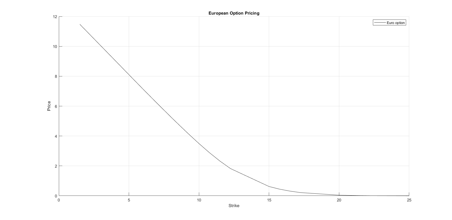
Figure 1: Pricing of European call option for $T=1,S_{0}=5$ and the function $J_{t,z}=z$ with Guassian jump distribution.

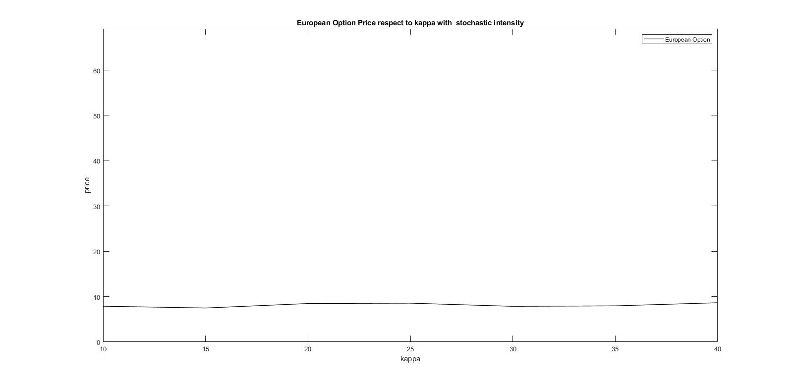
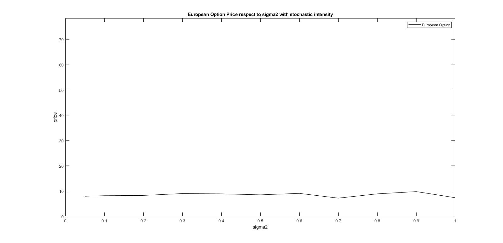
Figure 2: sensitivity of price with respect to k

Figure 3: sensitivity of price with respect to sigma2

5.1 Delta in the first and second approach

Figures 5 and 5 show the behaviour of these four expressions $\Delta$, $\Delta^{W}$, $\Delta^{N}$ and $\Delta^{W}/2+\Delta^{N}/2$ for $\sigma_{1}=0.10$, $\sigma_{2}=0.05$, $\Theta=0.30$, $\kappa=0.05$, $\mu=0.01$, $T=1$, $\lambda_{0}=0.10$, $S_{0}=5$, $K=S_{0}\times 1.2$ and time discretization $h=0.0001$. The jumps are generated by a normal distribution with a mean of $-0.10$ and a standard deviation of $0.50$ which satisfies Condition H1. The exact solution is $0.0481509$. The execution time of the program code in Malliavin method and finite difference method in the first approach are $2.2104\times 10^{4}$ and $4.4111\times 10^{4}$, and in the second approach are $2.2817\times 10^{4}$ and $4.5626\times 10^{4}$ respectively. The specifications of the computer system with which the program is implemented are Intel(R) Core i$7-9700$K CPU and $64$ GB Memory.

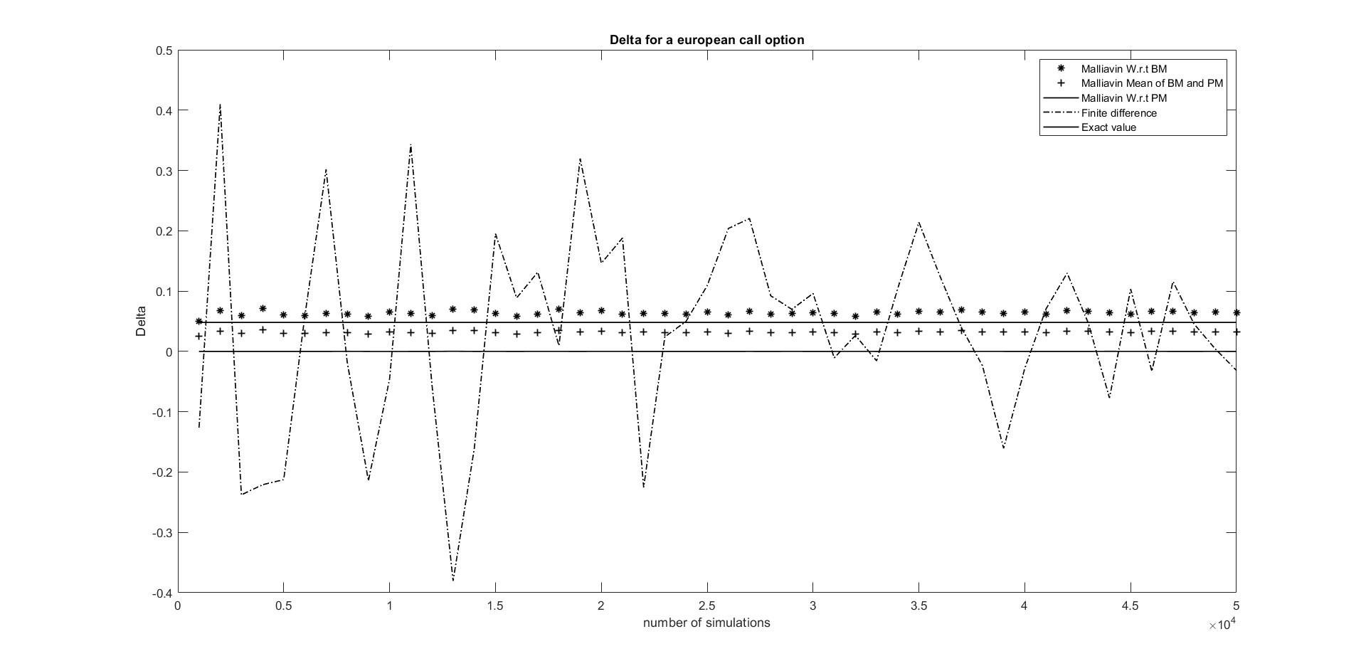
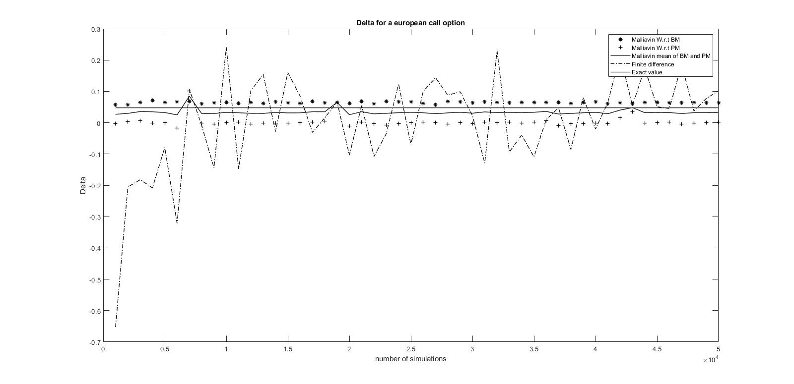
Figure 4: Greek Delta for European call option in the first approach for $J_{t,z}=z$ and Gaussian jump distribution.

Figure 5: Greek Delta for European call option in the second approach for $J_{t,z}=z$ and Gaussian jump distribution.

Table 1: The mean square error of four methods

$The\ Method$	$MSE\ of\ the\ first\ approach$	$MSE\ of\ the\ second\ approach$
$Winner-Malliavin(W_{M})\ Weight$	$0.0004$	$0.0003$
$Poisson-Malliavin(P_{M})\ Weight$	$0.0023$	$0.0021$
$Mean\ W_{M}\ and\ P_{M}\ Weight$	$0.0003$	$0.0002$
$Symmetric\ Finite\ Difference$	$0.0254$	$0.0190$

6 Funding

This work is based upon research funded by Iran National Science Foundation(INSF) under project No.4022879.

7 Conclusions

The main purpose of this article is to study the pricing of financial derivatives and to calculate the delta of them in a stochastic model with stochastic jump and intensity by using the Mallivain calculation. In the presence of the Malliavin derivative of the intensity, some Wiener-direction is found to be used in the duality formula of the Gaussian case appeared in calculating the delta and the price of financial derivatives. This subject, delta computation, is also considered in Poisson space with two different approaches. Finally, through the numerical results, we compare the price sensitivity computation in two methods, the finite difference method and the Malliavin method, with the exact solution in the models with jumps and stochastic intensity on asset prices and financial derivatives. The method developed in this paper can be extended to other pricing problems and Greeks associated with stochastic volatility processes and fractional Brownian motion. We leave these problems for our future work.

8 Acknowledgments

We wish to thank the referees for their valuable suggestions and comments which will have improved the paper.

References

• [Alos and Ewald(2008)] Alós, E., & Ewald, C-O., (2008). Malliavin differentiability of the Heston volatility and applications to option pricing, Adv. Appl. Prob., 40, 144–162.
• [Altmayer and Neuenkirch(2015)] Altmayer, M., & Neuenkirch, A., (2015). Multilevel Monte Carlo Quadrature of Discontinuous Payoffs in the Generalized Heston Model Using Malliavin Integration by Parts, Siam J. Financial Math., 6, 22–52.
• [Bavouzet and Messaoud(2006)] Bavouzet, M. P., & Messaoud, M. (2006). Computation of Greeks using Malliavin’s calculus in jump type market models, Electronic Journal of Probability, 11, 276–300.
• [Bezborodov et al.(2019)] Bezborodov, V., Di Persio, L., & Mishura, Y. ( 2019). Option pricing with fractional stochastic volatility and discontinuous payoff function of polynomial growth, Methodology and Computing in Applied Probability, 21, 331–366.
• [Bianchi and Fabozzi(2015)] Bianchi, M. L.,& Fabozzi, F. J. (2015). Investigating the performance of non-Gaussian stochastic intensity models in the calibration of credit default swap spreads, Computational Economics, 46, 243–273.
• [Bo et al.(2010)] Bo, L., Wang, Y., & Yang, X. (2010). Markov-modulated jump–diffusions for currency option pricing, Insurance: Mathematics and Economics, 46(3), 461–469.
• [Brèmaud(2020)] Brèmaud, P. (2020). Point Process Calculus in Time and Spaces: An Introduction with Applications, Springer Nature Switzerland.
• [Brigo and Alfonsi(2005)] Brigo, D., &Alfonsi, A., (2005). Credit default swap calibration and derivatives pricing with the SSRD stochastic intensity model, Finance and Stochastics, 9(1), 29–42.
• [Brigo and El-Bachir(2006)] Brigo, D., & El-Bachir, N. (2006). Credit derivatives pricing with a smile-extended jump stochastic intensity model, Available at SSRN 950208.
• [Chang et al.(2013)] Chang, C., Fuh, C-D., & Lin, S-K. (2013). A tale of two regimes: Theory and empirical evidence for a Markov-modulated jump diffusion model of equity returns and derivative pricing implications, Journal of Banking and Finance, 37, 3204–3217.
• [Chang and Wang(2020)] Chang, Y., & Wang, Y. (2020). Option pricing under double stochastic volatility model with stochastic interest rates and double exponential jumps with stochastic intensity, Mathematical Problems in Engineering.
• [Coffie et al.(2021)] Coffie, E., Duedahl, S., & Proske, F. (2021). Sensitivity Analysis with respect to a Stock Price Model with Rough Volatility via a Bismut-Elworthy-Li Formula for Singular SDEs, arXiv preprint arXiv:2107.06022.
• [El-Khatib and Privault(2004)] El-Khatib, Y., & Privault, N. (2004). Computations of Greeks in a market with jumps via the Malliavin calculus, Finance and Stochastics, 8(2), 161–179.
• [Elliott et al.(2007)] Elliott, R. J., Siu, T., Chan, K. L., & Lau, J. W. (2007). Pricing Options Under a Generalized Markov-Modulated Jump-Diffusion Model, Stochastic Analysis and Applications, 25(4), 821–843.
• [Fang(2000)] Fang, H. (2000). Option pricing implications of a stochastic jump rate, University of Virginia, Working paper.
• [Feng(2017)] Feng, Y. (2017). CVA under Bates model with stochastic default intensity, Journal of Mathematical Finance, 7(3), 682–698.
• [Fournié et al.(2001)] Fournié, E., Lasry, J-M., Lebuchoux, J., & Lions, P-L. (2001). Applications of Malliavin calculus to Monte-Carlo methods in finance. II, Finance and Stochastics, 5(2), 201–236.
• [Hawkes(1971)] Hawkes, A. G. (1971). Spectra of Some Self-Exciting and Mutually Exciting Point Processes, Biometrika, 58(1), 83–90.
• [Hillairet et al.(2018)] Hillairet, C., Jiao, Y., & Réveillac, A. (2018). Pricing formulae for derivatives in insurance using Malliavin calculus, Probability, Uncertainty and Quantitative Risk, 3(1), 1–19.
• [Huang et al.(2014)] Huang, J., Zhu, W., & Ruan, X. (2014). Option pricing using the fast Fourier transform under the double exponential jump model with stochastic volatility and stochastic intensity, Journal of Computational and Applied Mathematics, 263, 152–159.
• [Hudde and Rüschendorf(2023)] Hudde, A., & Rüschendorf, L. (2023). European and Asian Greeks for Exponential Lévy Processes, Methodology and Computing in Applied Probability, 25(1), 39.
• [Huehne(2005)] Huehne, F. (2005). Malliavin calculus for the computation of Greeks in markets driven by pure-jump Lévy processes, Available at SSRN 948347.
• [Khedher(2012)] Khedher, A. (2012). Computation of the delta in multidimensional jump-diffusion setting with applications to stochastic volatility models, Stochastic Analysis and Applications, 30(3), 403–425.
• [Kuchuk-Iatsenko et al.(2016)] Kuchuk-Iatsenko, S., Mishura, Y., & Munchak, Y. (2016). Application of Malliavin calculus to exact and approximate option pricing under stochastic volatility, arXiv preprint arXiv:1608.00230.
• [Leung and Kwok(2009)] Leung, K. S., & Kwok, Y. Y. (2009). Counterparty risk for credit default swaps: Markov chain interacting intensities model with stochastic intensity, Asia-Pacific Financial Markets, 16, 169–181.
• [Lévy dit Véhel and Lévy Véhel(2018)] Lévy dit Véhel, P. E., & Lévy Véhel, J. (2018). Stochastic jump intensity models, Risk and Decision Analysis, 7(1-2), 63–75.
• [Ma et al.(2023)] Ma, Y., Chen, L., & Lyu, J. (2023). Option valuation under double exponential jump with stochastic intensity, stochastic interest rates and Markov regime-switching stochastic volatility, Communications in Statistics-Theory and Methods, 52(7), 2043–2056.
• [Matchie(2009)] Matchie, L. (2009). Malliavin Calculus and Some Applications in Finance, African Institute for Mathematical Sciences (AIMS), South Africa.
• [Menaldi(2008)] Menaldi, J-L. (2008). Stochastic differential equations with jumps, Internet Publication, First Version.
• [Mhlanga(2011)] Mhlanga, F. J. (2011). Computation of Greeks using Malliavin calculus, Ph.D. thesis, University of Cape Town.
• [Nualart(2000)] Nualart, D. (2000). The Malliavin Calculus and Related Topics, Springer.