Floquet geometric entangling gates in ground-state manifolds of Rydberg atoms

Abstract

We propose an extension of the Floquet theory for constructing quantum entangling gates in ground-state manifolds of Rydberg atoms. By dynamically controlling periodically modulating the Rabi frequencies of transitions between ground and Rydberg states of atoms, error-resilient two-qubit entangling gates can be implemented in the regime of Rydberg blockade. According to different degrees of Floquet theory utilization, the fidelity of the resulting controlled gates surpasses that of the original reference. Our method only uses encoding in the ground states, and compared to the original scheme using Rydberg state for encoding, it is less susceptible to environmental interference, making it more practical to implement. Therefore, our approach may have broader applications or potential for further expansion of geometric quantum computation with neutral atoms.

Keywords: Rydberg atoms, quantum computation, Floquet engineering, geometric phase

1 Introduction

As one of the main themes in physics of this century, the geometric phase [1, 2, 3, 4] has received much attention in quantum computing. Quantum computing can provide more efficient solutions than traditional computers in areas such as prime factorization [5, 6, 7] and machine learning [8, 9, 10]. Because a geometric phase depends only on the evolution path, quantum gates constructed through geometric phases have better anti-internal noise interference ability [11, 12, 13, 14, 15]. The geometric phase theory of quantum systems is the foundation of various patterns of geometric quantum computation. Starting from the seminal adiabatic geometric quantum computation(GQC) [16, 17, 18, 19] based on Berry phases and adiabatic holonomic quantum computation [20, 21, 22] based on adiabatic non-Abelian geometric phases, it has gradually developed to include nonadiabatic geometric quantum computation(NGQC) [23, 24, 25, 26, 27, 28, 29] based on nonadiabatic Abelian geometric phases, and non-adiabatic holonomic geometric quantum computation(NHQC) [30, 31, 32, 33, 34, 35, 36, 37, 38, 39, 40, 41, 42, 43] based on nonadiabatic non-Abelian geometric phases. Due to the limited ability of these non-adiabatic gates to address laser control errors, to tackle this issue, the application of periodic control pulses in the GQC scenario is gradually increasing [44, 45, 46, 47].

Recently, a new computing scheme, Floquet geometric quantum computation (FGQC) [48], has gained significant attention, where universal error-resistant geometric gates can be constructed via a non-Abelian geometric phase. FGQC has recently been demonstrated in experiments with utracold atoms [49]. However, although the original Floquet two-qubit scheme using atomic Rydberg states for encoding qubits can achieve gate operations in a single step, Rydberg states are necessarily manipulated in low-temperature and high-vacuum environments, which means they are highly sensitive to external interference and may affect the accuracy of computational results. In contrast, if two of atomic ground states are used for encoding qubit, they are easier to prepare and control than Rydberg states, making the gate implementation simpler, less sensitive to external interference, more feasible in practical applications.

In this paper, we apply Floquet theory to construct two-qubit geometric entangling gates in ground-state manifolds of Rydberg atoms in the regime of Rydberg blockade [50, 51, 52, 53, 54]. The performances of resulting quantum gates are analyzed with respect to different degrees of Floquet engineering, decay rate, and different quantum gates. We compare the proposed Floquet gate scheme with the original one, and perform numerical simulations in the presence of certain system control errors. The numerical results indicate that, compared with the reference Rydberg-state Floquet gate, the present ground-state Floquet gate can gain higher fidelity and better robustness to control errors. When ignoring the atomic decay, using the Floquet scheme for both the control and target qubits will achieve higher fidelity and robustness. When there is a decay rate, using the Floquet scheme only for the target qubit will achieve higher fidelity while maintaining higher robustness. In addition, the controlled phase gate has high robustness to decay rates, which has been analyzed and demonstrated in the article.

This paper is organized as follows: In Sec. 2, we analyzed the general theory of Floquet geometric entangling gates in the regime of Rydberg blockade. In Sec. 3, we introduced and derived two new schemes with the Floquet scheme in Rydberg-blockade gates, demonstrating the feasibility of the proposed schemes. In Sec. 4, we select two sets of possible parameters, providing numerical simulations for both corresponding schemes to validate their performance. We examine the robustness with respect to Rabi error $\delta$ and the fidelity in different schemes for CNOT and CT gates. Subsequently, we analyze the impact of spontaneous emission on the gate schemes, identify the relatively superior scheme in each scenario, and offer optimization suggestions. The conclusion is presented in Sec. 5.

2 Physical model with two Rydberg atoms

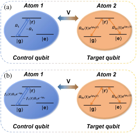
Figure 1: Energy level diagram of two Rydberg atoms with RRI strength $V$ for constructing the two-qubit entangling gates in (a) scheme A and (b) scheme B.

Consider a two-atom system where two atoms interact with each other through the van der Waals Rydberg-Rydberg interaction (RRI). For constricting a conditioned two-qubit entangling gate, we specify the control and target qubits, as shown in figures 1(a) and 1(b). The two atoms have two ground states $|g\rangle$ and $|e\rangle$ encoding qubits and a Rydberg state $|r\rangle$ mediating RRI between the permanent dipole moments of Rydberg states excited by a constant electric field, which are far greater than the laser Rabi frequency, to entangle atoms.

To implement gate operations under distributed laser control, we conduct a three-step scheme in the regime of Rydberg blockade. (i) Apply a $\pi$-pulse on the control qubit to induce the atomic transition from the ground $|g\rangle$ to the Rydberg state $|r\rangle$, with Rabi frequency $\Omega$. (ii) Apply pulses on the target qubit that drives separately the transitions from $|g\rangle$ and $|e\rangle$ states to the Rydberg state, with time-dependent Rabi frequencies $\Omega_{0r}$(t) and $\Omega_{1r}$(t), respectively. (iii) Apply a $-\pi$-pulse on the control qubit to deexcite the atom from the Rydberg state to the ground state $|g\rangle$, with a Rabi frequency $-\Omega$. For the system remaining in the Rydberg blockade regime, the a strong RRI strength is assumed $V\gg\Omega$, $\Omega_{0r}(t)$, $\Omega_{1r}(t)$. In the Rydberg blockade regime, the system Hamiltonian containing the three steps can be written as

$$H(t) = \frac{\Omega_{1}}{2}|g\rangle_{1}\langle r|\otimes\mathbb{I}+\frac{\Omega_{0r}(t)}{2}e^{i\varphi_{0}(t)}|e\rangle_{1}\langle e|\otimes|g\rangle_{2}\langle r|$$ (1)

$$+\frac{\Omega_{1r}(t)}{2}e^{i\varphi_{1}(t)}|e\rangle_{1}\langle e|\otimes|e\rangle_{2}\langle r|+{\rm H.c.}$$

$\mathbb{I}$ is the identity operator acting on the Rydberg atom.

To achieve a Floquet two-qubit gate, we introduce a periodic function $f(t)=\cos(wt)$ and a constant $\theta$, and set $\Omega_{0r}(t)=\sin(\theta/2)f(t)\Omega_{0}$ and $\Omega_{1r}(t)=\cos(\theta/2)f(t)\Omega_{0}$. Then the laser pulses of target qubit can be written as $\Omega(t)=\sqrt{{\Omega}^{2}_{0r}(t)+{\Omega}^{2}_{1r}(t)}=f(t)\Omega_{0}$, where $\tan(\theta/2)=\Omega_{0r}$(t)/ $\Omega_{1r}$(t). Expressing $|g\rangle\otimes|e\rangle$ in a reduced form $|ge\rangle$, then rewrite the Hamiltonian in Eq. (1) as

$$H_{f}(t) = \frac{\Omega_{1}}{2}|g\rangle_{1}\langle r|\otimes\mathbb{I}+\frac{f(t)}{2}\Omega_{0}[\sin\frac{\theta}{2}e^{i\varphi_{0}(t)}|eg\rangle\langle er|+\cos\frac{\theta}{2}e^{i\varphi_{1}(t)}|ee\rangle\langle er|]$$ (2)

$$+{\rm H.c.}$$

Based on this Hamiltonian, we next show two different schemes to implement Floquet geometric entangling gates in the Rydberg blockade regime.

3 Floquet geometric entangling gates

In former scheme of FGQC [48], the qubit contain a Rydberg state, for which such an encoding way makes it easier to achieve coupling between qubits but makes the quantum gates more susceptible to environmental interference compared to the gates with ground-state qubits, because Rydberg states would suffer higher decoherence rates and have a relatively shorter lifetime. Moreover, It requires precise experimental conditions and a high degree of control accuracy to manipulate Rydberg states, demanding advanced experimental equipment and techniques. Therefore, here we utilize two ground states to encode qubit states as $|0\rangle\equiv|g\rangle$ and $|1\rangle\equiv|e\rangle$ respectively, with the state $|r\rangle$ serving solely as an intermediate state rather than a computational state. Simultaneously providing $\mathbb{I}=|0\rangle\langle 0|+|1\rangle\langle 1|$, then we can obtain

$$H(t) = \frac{\Omega_{1}}{2}(|00\rangle\langle r0|+|01\rangle\langle r1|)+\frac{f(t)}{2}\Omega_{0}\left[\sin\frac{\theta}{2}e^{i\varphi_{0}(t)}|10\rangle\langle 1r|\right.$$ (3)

$$+\left.\cos\frac{\theta}{2}e^{i\varphi_{1}(t)}|11\rangle\langle 1r|\right]+{\rm H.c.}$$

3.1 Scheme A: Target-qubit Floquet engineering

In this scheme, we combine the standard dynamical gate (DG) with FGQC, referred to DG-FGQC. In steps (i) and (iii), we employ the DG method, while in step (ii), we utilize Floquet theory. We initially apply the $\pi$ pulses $\Omega_{1}$, resonant with the transition frequency between $|0\rangle$ and $|r\rangle$, in a square wave form on the control qubit. The state $|1\rangle$ is not affected by the laser. If the control qubit is initially in the state $|0\rangle$, the pulse sequence $\Omega_{1}$ will bring the control qubit to the Rydberg state, while no change occurs if the initial state of the control qubit is $|1\rangle$. The pulse duration is $T_{1}=\pi/\Omega_{1}$. Then moving on to the target qubit, due to the presence of RRI, within the Rydberg blockade regime $V\gg\Omega_{0}$, the target qubit cannot be excited to the Rydberg state when the control qubit is initially in the state $|0\rangle$. When the control qubit is initially in the state $|1\rangle$, the Hamiltonian on the target state in the second step is

$$H_{t}(t)=\frac{f(t)}{2}\Omega_{0}e^{i\varphi_{1}(t)}\left[\sin\frac{\theta}{2}e^{i\varphi(t)}|0\rangle+\cos\frac{\theta}{2}|1\rangle\right]\langle r|+{\rm H.c.},$$ (4)

with $\varphi_{0}(t)=\varphi_{1}(t)+\varphi(t)$. Then we can define a bright state $|b\rangle=\sin(\theta/2)e^{i\varphi(t)}|0\rangle+\cos(\theta/2)|1\rangle$, and a decoupled dark state $|d\rangle=\cos(\theta/2)e^{i\varphi(t)}|0\rangle-\sin(\theta/2)|1\rangle$ [55]. Obviously, the effective Hamiltonian only affects the subspace $S=Span\left\{|b\rangle,|r\rangle\right\}$, and then the Hamiltonian (4) can be rewritten as follows

$$H_{t}(t)=f(t)F\cdot n(t),$$ (5)

where $F\equiv\left(\tilde{\sigma}_{x},\tilde{\sigma}_{y},\tilde{\sigma}_{z}\right)^{T}/2$ being the spin operators on the subspace $S$ and $n(t)\equiv\Omega_{0}\left(\cos\varphi_{1}(t),-\sin\varphi_{1}(t),0\right)^{T}$ is the unit vector. According to reference [48], we select $R(t)=\exp[-i\Omega_{0}\sin(wt)F\cdot n(t)/w]$, which satisfies the boundary condition $R(\tau)=R(0)=\mathbb{I}$, if $\omega\tau=k\pi,\forall k\in\mathbb{N}^{+}$, yielding

$$H_{t}(t)=\dot{\varphi}(t)R^{\dagger}(t)(-i\partial/\partial\varphi)R(t),$$ (6)

When considering $w\gg\dot{\varphi}(t)$, we have an effective Hamiltonian [45]

$$H_{\rm eff}(t)=[1-J_{0}(\Omega_{0}/w)]F\cdot[n(t)\times\dot{n}(t)]/\Omega_{0}^{2},$$ (7)

with $J_{0}$ being zeroth-order Bessel function of the first kind. Set $\varphi_{1}(t)=Nt$, and then from the evolution operator $U\approx\mathcal{T}e^{-i\int_{0}^{\tau}H_{\rm eff}(t)dt}$ at time $t=\tau$, we get

$$U(\tau,0)=\left(\begin{array}[]{cc}e^{-iC\tau}&1\\ 1&e^{iC\tau}\\ \end{array}\right).$$ (10)

with $C\equiv$$-\left(N/2\right)\left[1-J_{0}(\Omega_{0}/w)\right]$, at the basis $\left\{|b\rangle,|r\rangle\right\}$ of the target qubit.

The dark state $|d\rangle$ is constructed to be orthogonal to the bright state, and it does not change after the laser changes the bright state. So we write the evolution operator as

$$U(\tau,0)=e^{-iC\tau}\left|b\right\rangle\langle b|+e^{iC\tau}\left|r\right\rangle\langle r|+\left|d\right\rangle\langle d|.$$ (11)

Here, since $\left|r\right\rangle$ serves as an auxiliary intermediate state uninvolved in the qubit states, we can rewrite Eq. (11) as

$$U(\tau,0)=e^{-iC\tau}\left|b\right\rangle\langle b|+\left|d\right\rangle\langle d|.$$ (12)

To obtain the control parameters for the target qubit, we transform the two-qubit basis vectors into $\left\{\left|10\right\rangle,\left|11\right\rangle\right\}$ and then obtain a new evolution matrix

$$U(\tau,0)=\left(\begin{array}[]{cc}e^{-iC\tau}\sin\left(\frac{\theta}{2}\right)^{2}+\cos\left(\frac{\theta}{2}\right)^{2}&e^{-iC\tau}\sin\theta\frac{e^{i\varphi}}{2}-\sin\theta\frac{e^{i\varphi}}{2}\\ e^{-iC\tau}\sin\theta\frac{e^{-i\varphi}}{2}-\sin\theta\frac{e^{-i\varphi}}{2}&e^{-iC\tau}\cos\left(\frac{\theta}{2}\right)^{2}+\sin\left(\frac{\theta}{2}\right)^{2}\\ \end{array}\right).$$ (15)

Then, we can choose suitable parameters to obtain the corresponding quantum gate for the target qubit. The laser action time for this process is $T_{2}$. Finally, perform another $-\Omega_{1}$ laser on the control bit for $T_{3}=\pi/\Omega_{1}$, which returns the control qubit to its initial state. When the control qubit is in the state $\left|0\right\rangle$, it will be excited to the Rydberg state after the first step, preventing the target qubit from reaching the excited state, which leads to the blocking of target qubit, rendering the gate $U(\tau,0)$ ineffective. Overall, a conditioned two-qubit geometric gate is constructed with form $U_{CU}=|0\rangle_{1}\langle 0|\otimes\mathbb{I}+|1\rangle_{1}\langle 1|\otimes U(\tau,0)$.

3.2 Scheme B: Two-qubit Floquet engineering

In this subsection, to simultaneously conduct Floquet engineering on the control and target qubits, we will augment the single-qubit FGQC scheme on basis of subsection 3.1 by incorporating the control qubit, which is referred to as FGQC-FGQC.

As the laser affecting the control qubit only influences the distribution of states $\left|g\right\rangle$ and $\left|r\right\rangle$ in the first step, we reduce the single-qubit three-level system to a two-level system with the Hamiltonian

$$H_{\rm ctrl}=\frac{\Omega_{1}}{2}|g\rangle\langle r|+{\rm H.c.}$$ (16)

for the control atom. To construct a single-qubit Floquet gate that transforms the control qubit from the ground state $\left|g\right\rangle$ to the excited state $\left|r\right\rangle$ and makes the system return to the initial state after a Floquet operation on the target qubit, we treat the $\left|r\right\rangle$ state as the computational state for analysis. We re-encode it, representing the $\left|g\right\rangle$ and $\left|r\right\rangle$ state as $\left|0\right\rangle$ and $\left|1\right\rangle$ states, respectively. Then we set the Floquet Hamiltonian

$$H_{\rm ctrl}^{\prime} = f_{1}\frac{\Omega_{1}}{2}e^{-i\varphi_{c}}|0\rangle\langle 1|+{\rm H.c.}$$ (17)

$$= f_{1}\frac{\Omega_{1}}{2}\left(\cos\varphi_{c}\sigma_{x}+\sin\varphi_{c}\sigma_{y}\right),$$

with $f_{1}=\cos(w_{1}t)$. In order to enable the construction of an X gate using Floquet, it needs to introduce a detuning term on the control qubit [48]. Then the Hamiltonian with detuning can be rewritten as

$$H_{f{\rm ctrl}} = f_{1}\frac{\Delta_{1}(t)}{2}\sigma_{z}+f_{1}\frac{\Omega_{1}(t)}{2}\left(\cos\varphi_{c}\sigma_{x}+\sin\varphi_{c}\sigma_{y}\right)$$ (18)

$$= f_{1}F_{0}\cdot r(t),$$

with $F_{0}=\left(\sigma_{x},\sigma_{y},\sigma_{z}\right)^{T}/2$ and the unit vector $r=\left(\Omega_{1}(t)\cos\varphi_{c},\Omega_{1}(t)\sin\varphi_{c},\Delta_{1}(t)\right)$. $\Delta_{1}(t)$ and $\Omega_{1}(t)$ are time-dependent parameters. Set $\Omega^{\prime}=\sqrt{\Omega_{1}^{2}(t)+\Delta_{1}^{2}(t)}$, and similarly, we obtain a Floquet effective Hamiltonian

$$H_{c{\rm eff}}=[1-J_{0}(\Omega^{\prime}/w_{1})]F\cdot[r(t)\times\dot{r}(t)]/\Omega^{\prime 2},$$ (19)

and then we can obtain the parameters of the X gate through the evolution operator $U\approx\mathcal{T}e^{-i\int_{0}^{\tau_{1}}H_{c{\rm eff}}(t)dt}$. Because equation (19) have the same form as equation (7), it can induce a single-qubit operation of matrix equation (15), making the atomic transition from $|g\rangle$ to $|r\rangle$, and vice versa. Combined with the second-step operation on the target qubit described in the scheme A, one can implement the FGQC-FGQC conditioned two-qubit entangling gate $U_{CU}=|0\rangle_{1}\langle 0|\otimes\mathbb{I}+|1\rangle_{1}\langle 1|\otimes U(\tau,0)$.

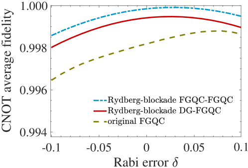
Figure 2: Comparison of the average fidelity for implementing a CNOT gate under three Floquet schemes.

4 Numerical simulations

In our approach, to obtain the desired two-qubit quantum gate, mainly to implement transformation in equation (15), we set $\varphi=0$ to obtain

$$U(\tau,0)=\left(\begin{array}[]{cc}e^{-iC\tau}\sin\left(\frac{\theta}{2}\right)^{2}+\cos\left(\frac{\theta}{2}\right)^{2}&e^{-iC\tau}\frac{\sin\theta}{2}-\frac{\sin\theta}{2}\\ e^{-iC\tau}\frac{\sin\theta}{2}-\frac{\sin\theta}{2}&e^{-iC\tau}\cos\left(\frac{\theta}{2}\right)^{2}+\sin\left(\frac{\theta}{2}\right)^{2}\\ \end{array}\right).$$ (22)

For example, we next conduct numerical simulations of implementing CNOT gates and CT gates. For the numerical simulations in the following, the Hamiltonians for the three steps are, respectively

$$H_{1} = \mathcal{F}\left[\frac{\Omega_{1}}{2}|g\rangle_{1}\langle r|+{\rm H.c.}+\frac{\Delta_{1}}{2}(|g\rangle_{1}\langle g|-|r\rangle_{1}\langle r|)\right]\otimes\mathbb{I}$$

$$H_{2} = \mathbb{I}\otimes f(t)\left[\frac{\Omega_{0r}(t)}{2}e^{i\varphi_{0}(t)}|g\rangle_{2}\langle r|+\frac{\Omega_{1r}(t)}{2}e^{i\varphi_{1}(t)}|e\rangle_{2}\langle r|+{\rm H.c.}\right]+V|rr\rangle\langle rr|$$

$$H_{3} = H_{1},$$ (23)

whith $\mathcal{F}=1$ and $\Delta_{1}=0$ [$\mathcal{F}=f_{1}$ and $\Delta_{1}=\Delta_{1}(t)$] for the DG-FGQC (FGQC-FGQC) gates.

4.1 Performances of CNOT and CT gates

For constructing a CNOT gate in three steps: (i) We first apply a laser pulse to the control qubit with $\Omega_{1}=2\times 2\pi$ MHz for a duration $T_{1}=0.25~{}{\rm\mu s}$. (ii) Considering the target qubit, set $\theta=-\pi/2$ and $e^{-iC\tau}=-1$ with $C\tau=-\pi$, $T_{2}=\tau$ being the duration of the second step, and $\omega\tau=k\pi,~{}\forall k\in\mathbb{N}^{+}$. Under the requirement of FGQC, we choose a set of feasible parameters $\Omega_{0}=\Omega_{1}$, $V=20\Omega_{0}$, $k=8$, $T_{2}=\tau=7.715~{}{\rm\mu s}$, and $w\approx 3.2576~{}{\rm MHz}$. (iii) Finally apply a laser pulse with $\Omega_{1}=-2\times 2\pi$ MHz to the control qubit for a duration of $T_{3}=0.25~{}{\rm\mu s}$.

In order to better measure the performance of the gate, we consider the average gate fidelity [56]

$$F(U,\varepsilon)=\frac{{\textstyle\sum_{j}}{\rm tr}\left[UU_{j}^{\dagger}U^{\dagger}\varepsilon(U_{j})\right]+d^{2}}{d^{2}(d+1)},$$ (24)

where $U$ represents the ideal logic gate, $U_{j}$ represents the tensor of Pauli matrices $\mathbb{I}$, $\sigma_{x}$, $\sigma_{y}$, $\sigma_{z}$ for single-qubit gate. Similarly, $U_{j}$ denotes $\mathbb{I}\otimes\mathbb{I}$, $\mathbb{I}\otimes\sigma_{x}$, $\mathbb{I}\otimes\sigma_{y}$, $\mathbb{I}\otimes\sigma_{z}$, $\cdots$, $\sigma_{z}\otimes\sigma_{z}$ for a two-qubit gate. Here $d=4$ for the two-qubit gate, and $\varepsilon(U_{j})$ denotes trace-preserving quantum operation. We set the relative Rabi error $\delta$ as a variable with $\delta\in\left[-0.1,0.1\right]$ to calculate the average fidelity, making the Rabi frequency deviations $\Omega_{0,1}(t)\rightarrow(1+\delta)\Omega_{0,1}(t)$. The resulting average fidelity for the DG-FGQC CNOT gate is shown by the curve labeled Rydberg-blockade DG-FGQC in figure 2. Additionally, for the FGQC-FGQC scheme, we follow $\Delta_{1}(t)=\sin(N_{1}t)\Omega^{\prime}$ and $\Omega_{1}(t)=\cos(N_{1}t)\Omega^{\prime}$ [48], and specify $\Omega^{\prime}=2\times 2\pi$ MHz, $\omega_{1}\approx 0.5133\times 2\pi$ MHz, $N_{1}\approx 45.728\times 2\pi$ kHz, $\tau_{1}\approx 7.797~{}{\rm\mu s}$, and $\varphi_{c}=\pi/2$. Accordingly, we have $T_{3}=T_{1}=\tau_{1}$, and the resulting average fidelity plot for the FGQC-FGQC CNOT gate is shown by the curve labeled Rydberg-blockade FGQC-FGQC in figure 2. At the same time, for reference we restored the fidelity of the two-qubit CNOT gate implemented with the original FGQC scheme [48], as shown by the curve labeled original FGQC in figure 2. By comparing the average fidelity curves under three different schemes, we find that applying the Floquet scheme in the Rydberg blockade regime performs better than the conventional approach. It exhibits higher fidelity and better robustness against the laser Rabi error, especially when both control and target qubits are operated with Floquet engineering.

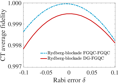
Figure 3: Comparison of the average fidelity for implementing a CT gate under three Floquet schemes.

For constructing a CT gate, the steps (i) to (iii) are similar to those for a CNOT gate. In the step (ii), considering the control qubit, we set $\theta=0$ and $e^{-iC\tau}=e^{i\pi/4}$. Due to $C=-\left(N/2\right)\left[1-J_{0}(\Omega_{0}/w)\right]$ and $\omega\tau=k\pi$, $\forall k\in\mathbb{N}^{+}$, we choose a set of feasible parameters with $k=2$, $T_{2}=\tau=1.157~{}{\rm\mu s}$, and $\omega\approx 5.41$ MHz. There are still $\Omega_{0}=\Omega_{1}$ and $V=20\Omega_{0}$. In the same way, we set the relative Rabi error $\delta$ to change the Rabi frequencies $\Omega_{0,1}(t)\rightarrow(1+\delta)\Omega_{0,1}(t)$. The resulting average fidelities for implementing the DG-FGQC and FGQC-FGQC CT gates are shown figure 3. The results indicate that, similar to the CNOT gate, the Floquet-engineering geometric CT gate can be implemented with high fidelity and excellent robustness against Rabi errors. Even when the relative Rabi error reaches $|\delta|=0.1$, the CT gate average fidelity is near 0.998. However, since the longer evolution time is required for implementing entangling gates by the Floquet engineering, it may not necessarily hold better performances when considering decay of atoms for the Floquet geometric gates. The following analysis will delve into this aspect.

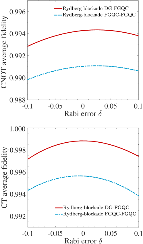
Figure 4: Impact of spontaneous emission on two different Floquet schemes for implementing (a) CNOT and (b) CT gates.

4.2 Floquet geometric entangling gate performance with atomic decay

We consider the dissipative dynamics of the system described by the following effective master equation [57]:

$$\frac{\partial\rho}{\partial t} = -i\left[\mathcal{H}_{I}\rho-\rho\mathcal{H}_{I}^{\dagger}\right]+\sum_{j=1}^{2}(\sigma_{0}^{j}\rho\sigma_{0}^{j\dagger}+\sigma_{1}^{j}\rho\sigma_{1}^{j\dagger}),$$

$$\mathcal{H}_{I} = H_{I}-\frac{i}{2}\sum_{j=1}^{2}(\sigma_{0}^{j}\sigma_{0}^{j\dagger}+\sigma_{1}^{j}\sigma_{1}^{j\dagger}),$$ (25)

in which $\rho$ is the density matrix of the system, and $H_{I}$ represents the system Hamiltonian given by equation (4).

Here we specify ⁸⁷Rb atoms as the qubit candidate, and the choose the atomic ground states $|g(e)\rangle=|5S_{1/2},F=1(2),m_{F}=0\rangle$ [58]. The Rydberg state is chosen as $|r\rangle=|97S,J=1/2,m_{J}=1/2\rangle$ [59] with the spontaneous emission rate being $\Gamma=2.48~{}{\rm kHz}$ at 300 K [60]. $\sigma_{0}^{j}=\sqrt{4\Gamma/13}\left|0\right\rangle_{j}\langle 1|$ and $\sigma_{1}^{j}=\sqrt{3\Gamma/13}\left|1\right\rangle_{j}\langle 1|$ describe the decay processes of the $j$th atom by effective spontaneous emission [55]. We analyze the impact of spontaneous emission and compare two different schemes for implementing the CNOT and CT gates, and the obtained results are shown in figure 4.

By comparing figure 4 and figures 2 and 3, it is evident that, although the fidelity and robustness to Rabi errors of the FGQC-FGQC scheme surpass the DG-FGQC scheme in the absence of dissipation, while when considering spontaneous emission, the fidelity of the FGQC-FGQC gate is lower that of the DG-FGQC gate. Meanwhile, the DG-FGQC scheme demonstrates better performance on robustness against Rabi errors, which is attributed to the high demands on the evolution time for FGQC, especially for CNOT gates, resulting in a significant impact of dissipation. In contrast, the DG-FGQC scheme only employs FGQC in the intermediate second step, which has a relatively minor impact. Therefore, it exhibits a preference for dissipation. To further investigate the impact of dissipation, we selected gates constructed using the superior DG-FGQC scheme for a comprehensive scan analysis under different decay rate.

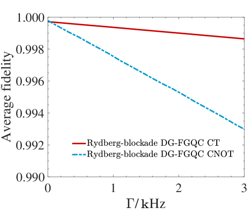
Figure 5: Effect of different atomic decay on fidelities of the DG-FGQC CT and CNOT gates.

Finally we consider effect of different decay rates of atoms on the fidelity of implementing Floquet entangling gates, corresponding to different situations with different atomic temperatures in experiment. In figure 5 we obtain the average fidelity of implementing DG-FGQC CNOT and CT gates with different atomic decay rates. Then we can get that DG-FGQC CT gate exhibits a certain resistance to atomic decay compared to the CNOT gate, which is attributed to the shorter Floquet evolution time of the CT gate compared to the CNOT gate, being only about 15$\%$ of the latter. As a matter of fact, overall the DG-FGQC entangling gates ae robust against atomic decay, because even when the decay rate reaches $\Gamma=3$ kHz the average fidelity of DG-FGQC entangling gates can be over 0.992.

5 Conclusion

In conclusion, we propose two-qubit entangling gate schemes with varying degrees of extension of Floquet theory in the Rydberg-blockade regime. Utilizing two three-level Rydberg atoms and employing time-dependent or time-independent driving fields acting stepwise on different atoms, numerical simulations demonstrate that our approach exhibits higher robustness to control errors and fidelity in addressing system control errors compared to traditional methods. Through simulations considering spontaneous emission, we find that the DG-FGQC scheme outperforms the FGQC-FGQC scheme in terms of robustness, particularly for phase gates with shorter evolution times. Additionally, compared to reference Floquet schemes encoding computational state on Rydberg states, our approach encodes qubits on the two ground states of atoms, demonstrating superior decoherence resistance and lower requirements on experimental conditions and control precision. Therefore, our scheme shows feasibility in the extension of Floquet theory.

References

References

- [1] Berry M V 1984 Proceedings of the Royal Society of London. A. Mathematical and Physical Sciences 392 45–57 URL https://royalsocietypublishing.org/doi/10.1098/rspa.1984.0023
- [2] Aharonov Y and Anandan J 1987 Physical Review Letters 58 1593 URL https://doi.org/10.1103/PhysRevLett.58.1593
- [3] Wilczek F and Zee A 1984 Physical Review Letters 52 2111 URL https://doi.org/10.1103/PhysRevLett.52.2111
- [4] Anandan J 1988 Physics Letters A 133 171–175 URL https://linkinghub.elsevier.com/retrieve/pii/0375960188910109
- [5] Vandersypen L M, Steffen M, Breyta G, Yannoni C S, Sherwood M H and Chuang I L 2001 Nature 414 883–887 URL https://www.nature.com/articles/414883a
- [6] Xu N, Zhu J, Lu D, Zhou X, Peng X and Du J 2012 Physical review letters 108 130501 URL https://link.aps.org/doi/10.1103/PhysRevLett.108.130501
- [7] Martin-Lopez E, Laing A, Lawson T, Alvarez R, Zhou X Q and O’brien J L 2012 Nature photonics 6 773–776 URL https://arxiv.org/abs/1111.4147
- [8] Rebentrost P, Mohseni M and Lloyd S 2014 Physical review letters 113 130503 URL https://journals.aps.org/prl/abstract/10.1103/PhysRevLett.113.130503
- [9] Li Z, Liu X, Xu N and Du J 2015 Physical review letters 114 140504 URL https://journals.aps.org/prl/abstract/10.1103/PhysRevLett.114.140504
- [10] Cong I, Choi S and Lukin M D 2019 Nature Physics 15 1273–1278 URL https://arxiv.org/abs/1810.03787
- [11] De Chiara G and Palma G M 2003 Physical review letters 91 090404 URL https://link.aps.org/doi/10.1103/PhysRevLett.91.090404
- [12] Zhu S L and Zanardi P 2005 Physical Review A 72 020301 URL https://link.aps.org/doi/10.1103/PhysRevA.72.020301
- [13] Leek P J, Fink J, Blais A, Bianchetti R, Goppl M, Gambetta J M, Schuster D I, Frunzio L, Schoelkopf R J and Wallraff A 2007 science 318 1889–1892 URL https://arxiv.org/abs/0711.0218
- [14] Filipp S, Klepp J, Hasegawa Y, Plonka-Spehr C, Schmidt U, Geltenbort P and Rauch H 2009 Physical review letters 102 030404 URL https://link.aps.org/doi/10.1103/PhysRevLett.102.030404
- [15] Berger S, Pechal M, Abdumalikov Jr A A, Eichler C, Steffen L, Fedorov A, Wallraff A and Filipp S 2013 Physical Review A 87 060303 URL https://link.aps.org/doi/10.1103/PhysRevA.87.060303
- [16] Jones J A, Vedral V, Ekert A and Castagnoli G 2000 Nature 403 869–871 URL https://pubmed.ncbi.nlm.nih.gov/10706278/
- [17] Wu L A, Zanardi P and Lidar D 2005 Physical review letters 95 130501 URL https://link.aps.org/doi/10.1103/PhysRevLett.95.130501
- [18] Wu H, Gauger E M, George R E, Möttönen M, Riemann H, Abrosimov N V, Becker P, Pohl H J, Itoh K M, Thewalt M L et al. 2013 Physical review A 87 032326 URL https://link.aps.org/doi/10.1103/PhysRevA.87.032326
- [19] Huang Y Y, Wu Y K, Wang F, Hou P Y, Wang W B, Zhang W G, Lian W Q, Liu Y Q, Wang H Y, Zhang H Y et al. 2019 Physical Review Letters 122 010503 URL https://link.aps.org/doi/10.1103/PhysRevLett.122.010503
- [20] Zanardi P and Rasetti M 1999 Physics Letters A 264 94–99 URL https://arxiv.org/abs/quant-ph/9904011
- [21] Duan L M, Cirac J I and Zoller P 2001 Science 292 1695–1697 URL https://arxiv.org/abs/quant-ph/0111086
- [22] Wu J L and Su S L 2019 Journal of Physics A: Mathematical and Theoretical 52 335301 URL https://dx.doi.org/10.1088/1751-8121/ab2a92
- [23] Xiang-Bin W and Keiji M 2001 Physical review letters 87 097901 URL https://link.aps.org/doi/10.1103/PhysRevLett.87.097901
- [24] Zhu S L and Wang Z 2002 Physical review letters 89 097902 URL https://link.aps.org/doi/10.1103/PhysRevLett.89.097902
- [25] Thomas J, Lababidi M and Tian M 2011 Physical Review A 84 042335 URL https://link.aps.org/doi/10.1103/PhysRevA.84.042335
- [26] Zhao P, Cui X D, Xu G, Sjöqvist E and Tong D 2017 Physical Review A 96 052316 URL https://link.aps.org/doi/10.1103/PhysRevA.96.052316
- [27] Li K, Zhao P and Tong D 2020 Physical Review Research 2 023295 URL https://link.aps.org/doi/10.1103/PhysRevResearch.2.023295
- [28] Chen T and Xue Z Y 2018 Physical Review Applied 10 054051 URL https://link.aps.org/doi/10.1103/PhysRevApplied.10.054051
- [29] Zhang C, Chen T, Li S, Wang X and Xue Z Y 2020 Physical Review A 101 052302 URL https://link.aps.org/doi/10.1103/PhysRevA.101.052302
- [30] Liu B J, Song X K, Xue Z Y, Wang X and Yung M H 2019 Physical Review Letters 123 100501 URL https://link.aps.org/doi/10.1103/PhysRevLett.123.100501
- [31] Sjöqvist E, Tong D M, Andersson L M, Hessmo B, Johansson M and Singh K 2012 New Journal of Physics 14 103035 URL https://iopscience.iop.org/article/10.1088/1367-2630/14/10/103035/meta
- [32] Xu G, Zhang J, Tong D, Sjöqvist E and Kwek L 2012 Physical review letters 109 170501 URL https://link.aps.org/doi/10.1103/PhysRevLett.109.170501
- [33] Xue Z Y, Zhou J and Wang Z 2015 Physical Review A 92 022320 URL https://link.aps.org/doi/10.1103/PhysRevA.92.022320
- [34] Xue Z Y, Gu F L, Hong Z P, Yang Z H, Zhang D W, Hu Y and You J 2017 Physical Review Applied 7 054022 URL https://link.aps.org/doi/10.1103/PhysRevApplied.7.054022
- [35] Zhou J, Liu B, Hong Z and Xue Z 2018 Science China Physics, Mechanics & Astronomy 61 1–7 URL https://link.springer.com/article/10.1007/s11433-017-9119-8
- [36] Hong Z P, Liu B J, Cai J Q, Zhang X D, Hu Y, Wang Z and Xue Z Y 2018 Physical Review A 97 022332 URL https://link.aps.org/doi/10.1103/PhysRevA.97.022332
- [37] Mousolou V A 2017 Physical Review A 96 012307 URL https://link.aps.org/doi/10.1103/PhysRevA.96.012307
- [38] Zhao P, Li K, Xu G and Tong D 2020 Physical Review A 101 062306 URL https://link.aps.org/doi/10.1103/PhysRevA.101.062306
- [39] Johansson M, Sjöqvist E, Andersson L M, Ericsson M, Hessmo B, Singh K and Tong D 2012 Physical Review A 86 062322 URL https://link.aps.org/doi/10.1103/PhysRevA.86.062322
- [40] Zheng S B, Yang C P and Nori F 2016 Physical Review A 93 032313 URL https://link.aps.org/accepted/10.1103/PhysRevA.93.032313
- [41] Ramberg N and Sjöqvist E 2019 Physical review letters 122 140501 URL https://link.aps.org/doi/10.1103/PhysRevLett.122.140501
- [42] Jing J, Lam C H and Wu L A 2017 Physical Review A 95 012334 URL https://link.aps.org/doi/10.1103/PhysRevA.95.012334
- [43] Liu B J, Wang Y S and Yung M H 2021 Physical Review Research 3 L032066 URL https://arxiv.org/pdf/2008.02176
- [44] Novičenko V, Anisimovas E and Juzeliūnas G 2017 Physical Review A 95 023615 URL https://link.aps.org/doi/10.1103/PhysRevA.95.023615
- [45] Novičenko V and Juzeliūnas G 2019 Physical Review A 100 012127 URL https://link.aps.org/doi/10.1103/PhysRevA.100.012127
- [46] Bomantara R W and Gong J 2018 Physical Review B 98 165421 URL https://link.aps.org/doi/10.1103/PhysRevB.98.165421
- [47] Bomantara R W and Gong J 2018 Physical Review Letters 120 230405 URL https://link.aps.org/doi/10.1103/PhysRevLett.120.230405
- [48] Wang Y S, Liu B J, Su S L and Yung M H 2021 Physical Review Research 3 033010 URL https://link.aps.org/doi/10.1103/PhysRevResearch.3.033010
- [49] Cooke L W, Tashchilina A, Protter M, Lindon J, Ooi T, Marsiglio F, Maciejko J and LeBlanc L J 2024 Physical Review Research 6 013057 URL https://journals.aps.org/prresearch/abstract/10.1103/PhysRevResearch.6.013057
- [50] Jaksch D, Cirac J I, Zoller P, Rolston S L, Côté R and Lukin M D 2000 Physical Review Letters 85 2208 URL https://link.aps.org/doi/10.1103/PhysRevLett.85.2208
- [51] Saffman M, Walker T G and Mølmer K 2010 Reviews of modern physics 82 2313 URL https://link.aps.org/doi/10.1103/RevModPhys.82.2313
- [52] Petrosyan D, Motzoi F, Saffman M and Mølmer K 2017 Physical Review A 96 042306 URL https://link.aps.org/doi/10.1103/PhysRevA.96.042306
- [53] Levine H, Keesling A, Omran A, Bernien H, Schwartz S, Zibrov A S, Endres M, Greiner M, Vuletić V and Lukin M D 2018 Physical review letters 121 123603 URL https://arxiv.org/abs/1806.04682
- [54] Wu J L, Wang Y, Han J X, Jiang Y, Song J, Xia Y, Su S L and Li W 2021 Phys. Rev. Appl. 16(6) 064031 URL https://link.aps.org/doi/10.1103/PhysRevApplied.16.064031
- [55] Sun L N, Yan L L, Su S L and Jia Y 2021 Physical Review Applied 16 064040 URL https://link.aps.org/doi/10.1103/PhysRevApplied.16.064040
- [56] Nielsen M A 2002 Physics Letters A 303 249–252 URL https://arxiv.org/abs/quant-ph/0205035
- [57] Rao D B and Mølmer K 2013 Physical review letters 111 033606 URL https://link.aps.org/doi/10.1103/PhysRevLett.111.033606
- [58] Zhang X L, Isenhower L, Gill A T, Walker T G and Saffman M 2010 Phys. Rev. A 82(3) 030306 URL https://link.aps.org/doi/10.1103/PhysRevA.82.030306
- [59] Li W, Viscor D, Hofferberth S and Lesanovsky I 2014 Phys. Rev. Lett. 112(24) 243601 URL https://link.aps.org/doi/10.1103/PhysRevLett.112.243601
- [60] Beterov I I, Ryabtsev I I, Tretyakov D B and Entin V M 2009 Phys. Rev. A 79(5) 052504 URL https://link.aps.org/doi/10.1103/PhysRevA.79.052504