Quantum Global Minimum Finder based on Variational Quantum Search

Abstract

The search for global minima is a critical challenge across multiple fields including engineering, finance, and artificial intelligence, particularly with non-convex functions that feature multiple local optima, complicating optimization efforts. We introduce the Quantum Global Minimum Finder (QGMF), an innovative quantum computing approach that efficiently identifies global minima. QGMF combines binary search techniques to shift the objective function to a suitable position and then employs Variational Quantum Search to precisely locate the global minimum within this targeted subspace. Designed with a low-depth circuit architecture, QGMF is optimized for Noisy Intermediate-Scale Quantum (NISQ) devices, utilizing the logarithmic benefits of binary search to enhance scalability and efficiency. This work demonstrates the impact of QGMF in advancing the capabilities of quantum computing to overcome complex non-convex optimization challenges effectively.

1 Introduction

Optimization challenges permeate a diverse range of fields, including science [1], engineering [2], and economics [3]. Central to these challenges is the quest to find the global minimum of a function, representing the most optimized state or solution within a given domain. Despite considerable research efforts [4, 5], accurately pinpointing global minimum in complex landscapes, characterized by multiple local minima, remains challenging. Traditional strategies, such as the brute-force approaches mentioned in [6, 7], necessitate traversing all elements in the search space, which becomes impractical for large datasets due to the "curse of dimensionality".

Alternative optimization techniques, including gradient-based [8], non-gradient-based [9], and genetic algorithms [10], offer strategies to navigate the search space more efficiently. Yet, these methods often fall short in guaranteeing the discovery of the global optimum, particularly in complex, non-convex functions [11] that pose the risk of trapping these algorithms in local optima.

Quantum computing emerges as a revolutionary paradigm, offering a novel approach to these longstanding optimization challenges. Unlike classical systems, which process information in binary bits, quantum systems utilize qubits, enabling the representation of multiple states simultaneously through superposition [12]. This capability allows quantum algorithms to explore vast search spaces more efficiently, potentially accelerating the discovery of global minimum for specific problem classes.

Among the quantum computing methodologies, Quantum Annealing (QA) has gained prominence for its potential in solving a subset of optimization problems known as "combinatorial optimization problems” [13]. QA leverages the principles of quantum mechanics to navigate the search space, aiming to converge on the global minimum by exploiting quantum tunneling and superposition. However, the practical application of QA is constrained by the need for adiabatic evolution [14] and faces challenges in guaranteeing solution optimality within realistic computational timeframes.

Grover’s algorithm [15] is a quantum algorithm that provides a quadratic speedup for searching unsorted databases, finding a specific item in $O(\sqrt{N})$ time, where $N$ is the number of items, compared to $O(N)$ time in classical computing. In [16], the author modified the Grover’s quantum algorithm [15] to solve real-world problems in identifying a global minimum, employing a relatively small number of quantum bits to find the global minimum. Despite the reduction to $O(\sqrt{N})$, the number of function evaluations still exhibits an exponential dependency on the number of qubits, given that $N=2^{n}$, where $n$ is the number of qubits.

Although Grover’s algorithm and the quantum amplitude amplification technique [17] provide quadratic speedup across various scientific and computational problems, their practical application faces limitations due to the exponential growth in quantum circuit complexity as more qubits are added. The advent of Variational Quantum Search (VQS) [18] introduces an innovative method that capitalizes on variational quantum algorithms and parameterized quantum circuits. VQS notably improves the odds of identifying desirable elements, while ensuring the maximal depth of quantum circuits increases linearly with the qubit count, a fact validated for systems up to 26 qubits.

This paper introduces the Quantum Global Minimum Finder (QGMF), an innovative quantum algorithm designed to efficiently locate the global minima of any given function, which is challenging due to potential multiple local optima. The QGMF algorithm combines a binary search technique with the VQS. Characterized by its low-depth circuit design, the QGMF is optimized for Noisy Intermediate-Scale Quantum (NISQ) hardware, leveraging the logarithmic advantage of binary search to enhance scalability and efficiency. This method represents an advance in tackling complex optimization problems across various fields by harnessing the power of quantum computing.

The remainder of the paper is structured as follows: Section 2 details the methodologies for data embedding, focusing on basis embedding and 2’s complement. In Section 3, we detail the QGMF, including its components such as quantum circuit, binary search, and VQS. Section 4 presents a complexity analysis and case study to evaluate the performance of the QGMF. Finally, Section 5 explores the broader implications of our findings and suggests directions for future research, while considering the limitations of the current study.

2 Data Embedding

This section outlines data embedding techniques in quantum computing, focusing on basis embedding and 2’s complement representation. It highlights the advantages of 2’s complement in simplifying arithmetic operations within quantum systems, providing a foundation for its application in the QGMF, especially detailed in Section 3.3. Furthermore, the 2’s complement described in this section provides a label qubit that is an essential input to VQS, a core part of QGMF, as described in Section 3.4.1.

Binary	Signed Magnitude	1’s complement	2’s complement
$|0000\rangle$	0	0	0
$|0001\rangle$	1	1	1
$|0010\rangle$	2	2	2
$|0011\rangle$	3	3	3
$|0100\rangle$	4	4	4
$|0101\rangle$	5	5	5
$|0110\rangle$	6	6	6
$|0111\rangle$	7	7	7
$|1000\rangle$	0	$-7$	$-8$
$|1001\rangle$	$-1$	$-6$	$-7$
$|1010\rangle$	$-2$	$-5$	$-6$
$|1011\rangle$	$-3$	$-4$	$-5$
$|1100\rangle$	$-4$	$-3$	$-4$
$|1101\rangle$	$-5$	$-2$	$-3$
$|1110\rangle$	$-6$	$-1$	$-2$
$|1111\rangle$	$-7$	0	$-1$

Table 1: Signed binary representations for 4-qubit encoding. It is evident that Signed Magnitude and 1’s complement have dual representations for the number $0$, which proves inefficient in arithmetic operations. The 2’s complement emerges as the standard method for encoding signed integer numbers in binary format [19].

2.1 Basis Embedding

In quantum computing, there are several ways to encode data like basis embedding, angle embedding, amplitude embedding, and so on [20]. In this paper, we used basis embedding. Basis embedding associates each input with a computational basis state of a qubit system. Therefore, data has to be in the form of binary strings. The embedded quantum state is the bit-wise translation of a binary string to the corresponding states of the quantum subsystems. For example, $x=0011$ is represented by the 4-qubit quantum state $|0011\rangle$.

2.2 2’s Complement Representation

Various methods exist for encoding signed integer numbers in binary representation, including Signed Magnitude, 1’s complement, and 2’s complement [19]. In Table 1, different representations of signed integer numbers encoded in a 4-qubit binary format are shown. 2’s complement serves as a fundamental method for representing signed integers in binary form and its format also ensures that the number $0$ has only one representation, making it unambiguous [19]. In this representation, the leftmost digit serves as the sign indicator: "0" signifies a positive number, and "1" denotes a negative number. Additionally, $p$ binary digits can accommodate a range of integer values ($R_{p}$) as defined in Eq. (1).

$$R_{p}=[-2^{p-1},2^{p-1}-1]$$ (1)

The concepts discussed are also applicable to the basis embedding of a 2’s complement quantum binary state $|x\rangle$, where the Most Significant Qubit (MSQ) signifies the sign of $|x\rangle$, in accordance with Eq. (2).

$$sign(|x\rangle)=|x\rangle_{MSQ}=\begin{cases}|0\rangle,&x\geq 0\\ |1\rangle,&x<0\end{cases}$$ (2)

Positive Numbers:

Converting a positive decimal integer $x$ to 2’s complement is straightforward, resembling the process for unsigned binary representation [19]. For example $\text{Decimal 5}\rightarrow|\text{0101}\rangle$.

Negative Numbers:

To convert negative decimal integer $x$ to 2’s complement, we use the procedure below:

1. Obtain the binary representation of the corresponding positive number ($-x$).

2. Invert all qubits (change 0s to 1s and vice versa).

3. Add 1 to the result.

For example, $\text{Decimal $-$5}\rightarrow|\text{$\overline{0101}$}+1\rangle=|1011\rangle$.

Addition and Subtraction:

In the 2’s complement, addition and subtraction operations mirror those of their unsigned counterparts, with a crucial consideration for the number of qubits required to accommodate the result. For instance, adding two 4-qubit numbers in 2’s complement demonstrates this:

$$\begin{array}[]{ccccc}&&\ |1010\rangle&\text{($-6$ in 4-qubit 2's complement)}\\ &+&\ |1101\rangle&\text{($-3$ in 4-qubit 2's complement)}\\ \hline\cr&&\ |0111\rangle&\text{(Incorrect positive result)}\end{array}$$

The mistaken positive result from adding two negative numbers highlights the inadequacy of 4 qubits for representing $-9$, which necessitates at least 5 qubits according to Eq. (1). By expanding the operands to 5 qubits we have:

$$\begin{array}[]{ccccc}&&\ |11010\rangle&\text{($-6$ extended to 5-qubit 2's complement)}\\ &+&\ |11101\rangle&\text{($-3$ extended to 5-qubit 2's complement)}\\ \hline\cr&&\ |10111\rangle&\text{($-9$ in 5-qubit 2's complement)}\end{array}$$

This adjustment accurately preserves the negative outcome, and the introduced qubit is termed an overflow qubit. Notably, in 2’s complement representation, extending a number necessitates the preservation of its sign, achieved by duplicating the MSQ before appending it, a rule named Sign Extension [19].

Thus, effectively conducting addition and subtraction in 2’s complement entails:

1. Converting all numbers to 2’s complement, ensuring uniform qubit length.

2. Avoiding overflow by adding necessary overflow qubits, e.g., adding two 4-qubit numbers may require a 5th qubit for accurate representation. Therefore, we need to have at least 5 qubits.

3. Finally, carry out addition or subtraction using these extended representations. Note that in this context, subtraction, expressed as "$a-b$", can be performed by adding "$a$" to the 2’s complement of "$b$".

Multiplication:

Suppose we have two numbers, $m$ and $k$, represented in unsigned binary format. We can express these numbers as $m=\sum_{i=0}^{n_{m}-1}m_{i}2^{i}$ and $k=\sum_{j=0}^{n_{k}-1}k_{j}2^{j}$, where, $m_{i}$ and $k_{j}$ are the individual qubits of $m$ and $k$, taking values from the set $\{0,1\}$, and $n_{m}$ and $n_{k}$ represent the number of qubits used to represent $m$ and $k$, respectively. The multiplication of $m$ and $k$ can be expressed as $m\cdot k=\sum_{i=0}^{n_{m}-1}\sum_{j=0}^{n_{k}-1}m_{i}k_{j}2^{i+j}$. To perform this multiplication in a way compatible with 2’s complement representation, we can follow these steps:

1. First, convert both $m$ and $k$ into their respective 2’s complement representations.

2. Next, expand the representation of both numbers by adding overflow qubits to make them each consist of $n_{m}+n_{k}$ qubits. Ensure that the added overflow qubits replicate the MSQ according to the sign extension rule.

3. After extending the representations, carry out the standard binary multiplication.

For example, consider a scenario where we have a 3-qubit binary number $m$ and a 4-qubit binary number $k$, and we wish to calculate the product $m\times k$. If $m=-2$ and $k=-3$, their binary representations would be $m=|110\rangle$ and $k=|1101\rangle$. Utilizing the sign extension rule and incorporating overflow qubits extends both numbers to 7 qubits. Thus, we get $m=|1111110\rangle$ and $k=|1111101\rangle$. In unsigned binary, these extended versions of $m$ and $k$ denote 126 and 125, respectively. When these numbers are multiplied in their unsigned form, the result is $m\times k=15750$. This product can be represented in a 7-qubit binary format as $|0000110\rangle$, which corresponds to 6 in 2’s complement notation.

3 Method: QGMF

This section details the QGMF, beginning with a high-level description to introduce the general concept and operational framework of the QGMF. It describes each component of the QGMF, including the quantum circuits used for an Oracle, a quantum adder, and the VQS. Additionally, the method incorporates a binary search technique to efficiently shift the objective function such that it helps VQS to effectively find the global minimum. The section also includes the pseudocode for the QGMF algorithm (Algorithm 1) and visual representations of the quantum circuits involved (Figure 2), offering a comprehensive guide to understanding and implementing the QGMF.

3.1 High-Level Description of QGMF

Assumption:

We consider an arbitrary function $f(x)$ without any restrictions on its properties, including convexity, continuity, differentiability, discreteness, etc.

Problem:

Our goal is to determine the global minimum ($G_{m}$) of the function $f(x)$ over a specific domain $D$.

Solution:

The idea is to determine $G_{m}$ through an iterative process, as depicted in Figure 1. In this approach, we shift the function $f(x)$ along the y-axis by an amount of $s_{i}$ in the $i$th iteration. This process continues until the number of negative values of $f(x)$ falls between 1 and a predefined threshold $T$, with the count of negative values determined by the VQS. Then we find the minimum of existing negative values ($M_{r}$) and utilize Eq. (3) to compute the global minimum.

$$G_{m}=M_{r}-s_{i}$$ (3)

It is important to note that the function $f(x)$ may be continuous and thus have an infinite number of values. Nevertheless, given that $f(x)$ is encoded through sampling, the count of evaluated $f(x)$ values becomes finite.

Figure 1: High-level overview of the QGMF algorithm for finding the global minimum of $f(x)$. In this specific example, since $f(x)$ is initially positive for all inputs, it needs to be shifted downward along the y-axis to generate negative values. This downward shift is accomplished by shifting the function by $s_{1}$. After the initial downward shift by $s_{1}$, the function produces a significant number of negative values (exceeding our specified threshold $T$), indicating the need for a smaller shift by $s_{2}$. Following this adjustment, the count of negative values of $f(x)+s_{2}$ becomes smaller than $T$, enabling us to easily identify the minimum among the remaining negative numbers denoted as $M_{r}$. Finally, we utilize Eq. (3) to calculate the value of $G_{m}$.

Conforming to the "quantum Church-Turing thesis" [21], it is conjectured that a quantum computer, given sufficient resources, can effectively simulate any classical computation and, in certain scenarios, execute it more efficiently than classical counterparts. Consequently, we can realize any classical function $f(x)$ as a quantum oracle $\hat{O}_{f}$, enabling the exploitation of quantum computing’s distinctive properties within QGMF.

To identify the global minimum of a classical function, it is essential to transform this function into a quantum oracle $\hat{O}_{f}$. This transformation has been the focus of various studies, such as those documented in [22], which explore methodologies for representing classical functions within quantum frameworks. Building upon this foundation, quantum arithmetic operations—highlighted in both [23] and our previous work [24]—introduce the capabilities for executing multiplication, addition, and averaging within a quantum domain. However, the efficient conversion of real-valued functions from $f(x)$ to $\hat{O}_{f}|x\rangle$ demands further exploration. Past research, including efforts by [25], has begun to tackle the complexities associated with quantum arithmetic for real-valued functions. Integrating these established techniques into our approach promises a robust pathway towards achieving our objective.

3.2 Defining the Oracle

To exploit quantum parallelism, we first apply Hadamard gates to create a uniform superposition of different inputs (Eq. (4)). This prepares a quantum state that encompasses all inputs simultaneously.

$$|\phi_{0}\rangle=H^{\otimes n}|0\rangle^{\otimes n}=\frac{1}{2^{\frac{n}{2}}}\sum_{x=0}^{2^{n-1}}|x\rangle$$ (4)

The next step in QGMF is to define the quantum oracle $\hat{O}_{f}$ which takes the input $|x\rangle$ and yields the output $|f(x)\rangle$ in 2’s complement format, as expressed in Eq. (5).

$$\hat{O}_{f}|x\rangle=|f(x)\rangle$$ (5)

The oracle is typically treated as a black-box quantum operator, with the objective of determining its global minimum while considering its output in 2’s complement representation.

To prevent overflow during the shifting phase, an additional overflow qubit was introduced immediately following the oracle. Utilizing a CNOT gate in conjunction with the MSQ entangles it with the MSQ, ensuring adherence to the 2’s complement conditions (e.g., sign extension) [19] (refer to section 2).

If needed, one can add any number of extra overflow qubits by following the same procedure. However, for our considerations, we assumed that $\hat{O_{f}}|x\rangle\subseteq[-2^{n-1},2^{n-1}-1]$. Additionally, given the worst-case scenario due to the lower and upper bounds of the shift $s_{i}$ in Algorithm 1, where $s_{i}\leftarrow\lfloor(Low+High)/2\rfloor$, we have $s_{i}\subseteq[-2^{n-1},2^{n-1}-1]$. Indeed, we need to accommodate the range $[-2^{n},2^{n}-2]$, requiring $n+1$ bits. Consequently, introducing one overflow qubit is sufficient.

By applying the oracle to the superposition of all potential inputs, we acquire a superposition of all oracle’s outputs, as outlined in Eq. (6), where $|\phi^{\prime}_{0}\rangle=\hat{O}_{f}|\phi_{0}\rangle$.

$$|\phi_{1}\rangle=|0\oplus|\phi^{\prime}_{0}\rangle_{MSQ}\rangle\otimes|\phi^{\prime}_{0}\rangle$$ (6)

3.3 Quantum Adder

The next step is implementing the adder circuit ("$A(s_{i})$") to add state $|\phi_{1}\rangle$ with the value $s_{i}$, which generates $|\phi_{2}(s_{i})\rangle=|\phi_{1}+s_{i}\rangle$. This can be achieved by using the Quantum Fourier Transform (QFT)-based adder [23]. Initially, we convert the state $|\phi_{1}\rangle$ from the computational basis to the Fourier basis by applying the QFT to it, resulting in a new state in the QFT basis denoted as $|\psi_{1}\rangle$ (see Eq. (7)).

$$|\psi_{1}\rangle=\mathrm{QFT}\left|\phi_{1}\right\rangle$$ (7)

Subsequently, Eq. (8) is employed to rotate the $j$-th qubit by an angle of $s_{i}\times\frac{\pi}{2^{j}}$ using the $R_{Z}$ gate. This rotation introduces a new phase of $(\phi_{1}+s_{i})\times\frac{\pi}{2^{j}}$ for the $j$-th qubit where $0\leq j\leq n$. The resulting state after these rotations is denoted as $|\psi_{2}(s_{i})\rangle$.

$$|\psi_{2}(s_{i})\rangle=R_{Z}(s_{i}\cdot\frac{\pi}{2^{0}})\left|\psi_{1}\right\rangle_{0}\otimes\ldots\otimes R_{Z}(s_{i}\cdot\frac{\pi}{2^{n}})\left|\psi_{1}\right\rangle_{n}$$ (8)

Finally, we apply $QFT^{-1}$ to return to the computational basis, yielding $|\phi_{2}(s_{i})\rangle$ as shown in Eq. (9).

$$|\phi_{2}(s_{i})\rangle=\mathrm{QFT}^{-1}|\psi_{2}(s_{i})\rangle\stackrel{{\scriptstyle\text{set}}}{{=}}|\phi_{1}+s_{i}\rangle$$ (9)

It is essential to underscore that the operator $A(s_{i})$ is designed to work exclusively with positive integers. However, in situations where the shift "$s_{i}$" is a negative integer, we need to perform a conversion from the 2’s complement form of the negative number to its positive decimal representation and then apply it to the $A$ operator. For example, if we intend to use $A(-2)$ with a 3-qubit configuration, we first convert $-2$ to its 2’s complement form, which is ${(110)}_{2}$, equivalent to $6$ in positive decimal notation. Consequently, we should utilize $A(6)$ in this scenario.

Algorithm 1   QGMF algorithm for finding the $G_{m}$ of $\hat{O}_{f}|x\rangle$.

1:Input:

2:      $\hat{O}_{f}:$ Quantum oracle in 2’s complement binary format

3:      $n:$ Number of qubits

4:      $T:$ Threshold $\geq 1$

5:Output:

6:      $G_{m}:$ Global minimum of $\hat{O_{f}}|x\rangle$

7:

8:$Low\leftarrow-2^{n-1}$

9:$High\leftarrow 2^{n-1}$

10:$i\leftarrow 0$

11:while True do

12:     $s_{i}\leftarrow\lfloor(Low+High)/2\rfloor$

13:     $\theta_{best}\leftarrow$ Run VQS on $|\phi_{2}(s_{i})\rangle$

14:     $results\leftarrow$ Measure the state $|\phi_{3}(s_{i},\theta_{\text{best}})\rangle$

15:     $N_{neg}\leftarrow$ Find the number of distinct negative values in $results$

16:     if $N_{neg}\in[1,T]$ then

17:         $M_{r}\leftarrow\min(results)$

18:         $G_{m}\leftarrow M_{r}-s_{i}$

19:         return $G_{m}$

20:     else if $N_{neg}>T$ then

21:         $Low\leftarrow s_{i}$

22:     else

23:         $High\leftarrow s_{i}$

24:     end if

25:     $i\leftarrow i+1$

26:end while

3.4 Variational Quantum Search and Binary Search

In the pursuit of the global minimum, we employ an iterative approach that combines binary search and VQS. In each iteration, the VQS is applied to search for the negative values of the shifted oracle, represented as $|\phi_{2}(s_{i})\rangle$ and shown in Figure 2. Subsequently, the number of negative values ($N_{neg}$) is used as a key metric for establishing the termination criteria of the binary search and for modifying its lower and upper limits. The binary search can help to quickly shift the position of the function, as illustrated in Figure 1, such that the $N_{neg}$ for the shifted function is between 1 and $T$, usually within several iterations.

3.4.1 Variational Quantum Search (VQS)

VQS is a variational quantum algorithm (VQA) proposed in [18]. As a variational alternative to Grover’s algorithm, VQS has undergone testing on searching unstructured databases comprising up to 26 qubits. The goal of VQS is to search good elements in an unstructured database, where the good elements’ label qubit in the VQS circuit is in state $|1\rangle$. VQS employs an Ansatz $U(\theta)$ from [18], which is optimized to transform the quantum state from a superposition of all elements to a superposition of solely good elements. The objective function in VQS is expressed as:

$$f_{\text{obj}}(\theta)=-0.5(\langle Z_{1}\rangle-\langle Z_{2}\rangle)$$ (10)

where $\langle Z_{1}\rangle$ and $\langle Z_{2}\rangle$ are measurements of two quantum circuits given in Figure 2, achieved by the Hadamard test [26], and can be expressed as Eqs. (11) and (12):

$$\langle Z_{1}\rangle=\langle\phi_{2}(s_{i})|U(\theta)|\phi_{2}(s_{i})\rangle$$ (11)

$$\langle Z_{2}\rangle=\langle\phi_{2}(s_{i})|Z\otimes I^{\otimes n}U(\theta)|\phi_{2}(s_{i})\rangle\text{.}$$ (12)

The MSQ of $|\phi_{2}(s_{i})\rangle$, given in Eq. (9), corresponds to the overflow qubit described in Section 2, and serves as the label qubit of VQS. When $U(\theta)$ is applied to this state, the resulting state is shown in Eq. (13).

$$|\phi_{3}(s_{i},\theta)\rangle=U(\theta)|\phi_{2}(s_{i})\rangle$$ (13)

(a)

(b)

Figure 2: Two quantum circuits used for the QGMF. (a) and (b) depict quantum circuits employed to measure $\langle Z_{1}\rangle$ and $\langle Z_{2}\rangle$, which are utilized in Eq. (10).

When the objective function specified in Eq. (10) reaches its global minimum, the parameters of the Ansatz also reach their optimal values, i.e., $\theta=\theta_{\text{best}}$, terminating the VQS iteration. At this point, the quantum state $|\phi_{3}(s_{i},\theta_{\text{best}})\rangle$ represents a superposition solely of the good elements, or equivalently, only the negative values of the oracle following the shift $s_{i}$. This state can also be expressed as Eq. (14), where $\beta_{j}$ represents the amplitude of the basis state $|y_{j}\rangle$, corresponding to the $j^{\text{th}}$ good element, or equivalently, the $j^{\text{th}}$ distinct negative value. Then, the count of negative values, denoted by $N_{\text{neg}}$, is determined by measuring the state $|\phi_{3}(s_{i},\theta_{\text{best}})\rangle$, i.e., this count is equal to the number of unique states measured.

$$|\phi_{3}(s_{i},\theta_{\text{best}})\rangle=\sum_{j=1}^{N_{neg}}\beta_{j}|y_{j}\rangle$$ (14)

3.4.2 Binary Search

We employ a binary search method, detailed in Algorithm 1, to optimize the shift value $s_{i}$ iteratively, aiming to refine our search for the global minimum effectively. The algorithm initiates by setting the shift $s_{i}$ to the midpoint between the current lower and upper bounds, defined as $2^{n-1}$ and $-2^{n-1}$, respectively, where $n$ represents the number of qubits.

In each iteration, we measure state $|\phi_{3}(s_{i},\theta_{\text{best}})\rangle$ as specified in Eq. (14) to determine the count of negative function values, denoted as $N_{neg}$. If the number of distinct negative values $N_{neg}^{(i)}$ exceeds a predefined threshold $T$, it suggests an excess of negative values, prompting an upward shift adjustment, and we assign the current $s_{i}$ to the lower bound of the subsequent iteration. Conversely, if $N_{neg}^{(i)}$ is approximately zero, indicating that the oracle outputs are predominantly above the x-axis, a downward shift is applied, and we assign the current $s_{i}$ to the upper bound of the subsequent iteration.

The binary search continues until $N_{neg}^{(i)}$ falls within the range of 1 to $T$, at which point the process is terminated, and the minimum value among the detected negative values, $M_{r}$, is identified. The global minimum $G_{m}$ is then calculated using $G_{m}=M_{r}-s_{i}$, given in Eq. (3). Note that the threshold $T$ is a small constant, leading to a constant time complexity of $O(T)$ for searching through the remaining negative oracle outputs.

4 Complexity Analysis and Case Study

This section delves into the complexity analysis and empirical simulation of the QGMF algorithm. Given that QGMF is a VQA, its performance metrics such as complexity and efficiency are influenced by several factors, including circuit depth, convergence rate, and number of measurements.

The adder circuit used in this paper consists of QFT and its inverse as well as one layer of Rz gates. Therefore, the complexity of the adder circuit, essential for shifting operations, is comparable to that of the QFT at time complexity of $O(n^{2}))$, where $n$ is the number of qubits [27]. The number of CR operations required for the QFT is $n(n+1)/2$. Furthermore, the VQS, playing a pivotal role in the local search phase, exhibits a linear depth complexity of $O(n)$, making it particularly well-suited for NISQ devices.

The optimization complexity, critical for identifying the optimal parameters of VQS, can be quantified based on the number of iterations and measurements. According to the findings documented in [18, 28], less than 300 iterations are necessary to achieve the desired state in most runs, highlighting the algorithm’s efficiency in parameter optimization. The number of measurements is twice the number of iterations.

Recent studies have confirmed the effectiveness of VQS in systems with up to 26 qubits, as detailed in [18, 28]. Efforts are currently underway to extend VQS capabilities to more qubits. For computational complexity analysis, it is important to recognize that in scenarios involving more than 26 qubits - where VQS’s efficiency has not yet been confirmed - Grover’s Search algorithm can be utilized as an interim solution. According to [15], this algorithm offers a quadratic speedup. Despite this advantage, preliminary analysis suggests that VQS could potentially outperform Grover’s algorithm in terms of circuit depth when applied to systems larger than 26 qubits. This suggests that the QGMF might achieve more than quadratic speedup in finding optimal solutions, indicating a promising avenue for further research in quantum computing efficiency.

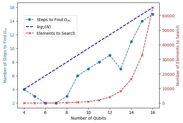
The outer loop of Algorithm 1 is a binary search, which is known to run in logarithmic time in the worst case. Therefore, we can expect the QGMF’s outer iteration can converge quickly, say within dozens of iterations, which is also supported by our experimental result given in Figure 3. The results given in this figure are obtained from simulation using Pennylane [20, 29]. Simulation tests indicate that the QGMF is as accurate as the classical brute-force method. As shown in Figure 3, the number of binary search steps required by the QGMF to locate the global minimum is within 15 for all the 13 cases we studied. These simulations assessed QGMF’s adaptability to different quantum oracles by encoding potential function values in quantum states. Each state involved a randomly generated, normalized input vector of dimension $2^{n}$, adhering to quantum circuitry norms. Detailed construction of the random oracles and comparisons with classical brute-force results are provided in Algorithm 2, underscoring the framework’s potential efficacy in quantum computing applications.

Figure 3: Efficiency of the QGMF in identifying the global minimum of randomly generated oracles, indicated by the number of binary search steps required (left vertical axis) across various qubit counts. It contrasts this with the volume of elements a classical brute-force search must navigate to achieve the same goal (right vertical axis). The function $\log_{2}{(N)}$, where $N$ is problem size, is also depicted.

5 Discussion

In this paper, we introduce the QGMF, an innovative approach designed to efficiently locate the global minimum of quantum oracles. The QGMF integrates a binary search with the VQS, harnessing quantum computing’s potential to outperform traditional brute-force methods significantly. Our analysis confirms the effectiveness of QGMF, demonstrating its superior performance in complex optimization scenarios. The implications of our study are profound, opening new avenues in fields such as finance, chemistry, and machine learning.

Future research will focus on evaluating QGMF under realistic quantum conditions, expanding its applications across various sectors, and refining quantum oracles to enhance their utility and performance. Despite its promising outcomes, we recognize the limitations of our current study, primarily the assumption of ideal quantum computing conditions which might not accurately represent the complexities faced in noisy quantum environments. Additionally, the scalability and practical deployment of QGMF in real-world applications require further exploration to fully realize its potential.

Appendix A Random Oracle Builder Function

Below is the pseudocode for the "Random Oracle Builder" function, illustrating the method used to generate the test vectors and their associated global minimum values for our analysis.

Algorithm 2 Random Oracle Builder

1:Input: $n$: Number of qubits

2:Output: $rand\_vec$: Normalized random vector, $G_{m}$: Global minimum

3:

4:$size\leftarrow 2^{n}$

5:$negative\_index\leftarrow\lfloor size/2\rfloor$

6:Initialize $rand\_vec$ as a zero vector of length $size$

7:$classical\_min\_index\leftarrow size+1$

8:$min\_index\_found\leftarrow$ False

9:Determine number of non-zero elements, $\#non\_zeros$

10:$indices\leftarrow$ randomly selected sorted indices from $size$, of length $\#non\_zeros$

11:for each $i$ in $indices$ do

12:     Assign a random value to $rand\_vec[i]$

13:     if not $min\_index\_found$ then

14:         if $i<negative\_index$ and $i<classical\_min\_index$ then

15:              $classical\_min\_index\leftarrow i$

16:         else if $i\geq negative\_index$ then

17:              $classical\_min\_index\leftarrow i$

18:              $min\_index\_found\leftarrow$ True

19:         end if

20:     end if

21:end for

22:Normalize $rand\_vec$

23:if $classical\_min\_index<negative\_index$ then

24:     $G_{m}\leftarrow classical\_min\_index$

25:else

26:     $sign\_bin\_rep\leftarrow$ 2’s complement of $classical\_min\_index$

27:     $G_{m}\leftarrow$ convert $sign\_bin\_rep$ to integer

28:end if

29:return $rand\_vec$, $G_{m}$

The significance of each vector element in representing function values is twofold: a zero element indicates an outcome not produced by the function, while a non-zero element signifies a possible value. The distribution of positive and negative values within these vectors reflects the function’s behavior across its domain. The detailed process of vector generation and its implications for identifying the function’s global minimum are captured in Algorithm 2, which also highlights the classical method used to benchmark the quantum findings.

Code Availability

The code supporting this study is available on GitHub at the following URL:
https://github.com/natanil-m/quantum_global_minimum_finder.

Data Availability

The datasets generated and/or analysed during the current study are available in the GitHub repository, https://github.com/natanil-m/quantum_global_minimum_finder.

References

- [1] Floudas, C. A. & Pardalos, P. M. State of the art in global optimization: computational methods and applications (Springer Science & Business Media, 2013).
- [2] Boyd, S., Vandenberghe, L. & Faybusovich, L. Convex optimization. \JournalTitleIEEE Transactions on Automatic Control 51, 1859–1859, DOI: 10.1109/TAC.2006.884922 (2006).
- [3] Dixit, A. K. Optimization in economic theory (Oxford University Press, USA, 1990). https://academic.oup.com/book/0/chapter/420796084/chapter-pdf/52079915/isbn-9780198772101-book-part-1.pdf.
- [4] Ge, R., Huang, F., Jin, C. & Yuan, Y. Escaping from saddle points—online stochastic gradient for tensor decomposition. In Conference on learning theory, 797–842 (PMLR, 2015).
- [5] Choromanska, A., Henaff, M., Mathieu, M., Arous, G. B. & LeCun, Y. The loss surfaces of multilayer networks. In Artificial intelligence and statistics, 192–204 (PMLR, 2015).
- [6] Mahoor, M., Salmasi, F. R. & Najafabadi, T. A. A hierarchical smart street lighting system with brute-force energy optimization. \JournalTitleIEEE Sensors Journal 17, 2871–2879 (2017).
- [7] Ploskas, N. & Sahinidis, N. V. Review and comparison of algorithms and software for mixed-integer derivative-free optimization. \JournalTitleJournal of Global Optimization 1–30 (2022).
- [8] Ruder, S. An overview of gradient descent optimization algorithms. arXiv:1609.04747 [cs.LG] (2017).
- [9] Larson, J., Menickelly, M. & Wild, S. M. Derivative-free optimization methods. \JournalTitleActa Numerica 28, 287–404, DOI: 10.1017/S0962492919000060 (2019).
- [10] Katoch, S., Chauhan, S. S. & Kumar, V. A review on genetic algorithm: past, present, and future. \JournalTitleMultimedia tools and applications 80, 8091–8126 (2021).
- [11] Clarke, F. H. Optimization and nonsmooth analysis (SIAM, 1990).
- [12] Knill, E. Quantum computing. \JournalTitleNature 463, 441–443 (2010).
- [13] Rajak, A., Suzuki, S., Dutta, A. & Chakrabarti, B. K. Quantum annealing: an overview. \JournalTitlePhilosophical Transactions of the Royal Society A: Mathematical, Physical and Engineering Sciences 381, DOI: 10.1098/rsta.2021.0417 (2022).
- [14] Albash, T. & Lidar, D. A. Adiabatic quantum computation. \JournalTitleRev. Mod. Phys. 90, 015002, DOI: 10.1103/RevModPhys.90.015002 (2018).
- [15] Grover, L. K. A fast quantum mechanical algorithm for database search. In Symposium on the Theory of Computing (1996).
- [16] Zhu, J., Huang, Z. & Kais, S. Simulated quantum computation of global minima. \JournalTitleMolecular Physics 107, 2015–2023, DOI: 10.1080/00268970903117126 (2009).
- [17] Brassard, G., Høyer, P., Mosca, M. & Tapp, A. Quantum amplitude amplification and estimation, DOI: 10.1090/conm/305/05215 (2002).
- [18] Zhan, J. Variational quantum search with shallow depth for unstructured database search. arXiv:2212.09505 [quant-ph] (2023).
- [19] Patterson, D. A. & Hennessy, J. L. Computer Organization and Design ARM Edition: The Hardware Software Interface (Morgan Kaufmann, 2016).
- [20] Bergholm, V. et al. Pennylane: Automatic differentiation of hybrid quantum-classical computations (2022). 1811.04968.
- [21] Bernstein, E. & Vazirani, U. Quantum complexity theory. \JournalTitleSIAM Journal on Computing 26, 1411–1473, DOI: 10.1137/S0097539796300921 (1997). https://doi.org/10.1137/S0097539796300921.
- [22] Häner, T., Roetteler, M. & Svore, K. M. Optimizing quantum circuits for arithmetic. arXiv:1805.12445 [quant-ph] (2018).
- [23] Ruiz-Perez, L. & Garcia-Escartin, J. C. Quantum arithmetic with the quantum fourier transform. \JournalTitleQuantum Information Processing 16, 1–14 (2017).
- [24] Zhan, J. Quantum multiplier based on exponent adder. arXiv:2309.10204 [quant-ph] (2023).
- [25] Seidel, R., Tcholtchev, N., Bock, S., Becker, C. K.-U. & Hauswirth, M. Efficient floating point arithmetic for quantum computers. \JournalTitleIEEE Access 10, 72400–72415 (2022).
- [26] Bravo-Prieto, C. et al. Variational Quantum Linear Solver. \JournalTitleQuantum 7, 1188, DOI: 10.22331/q-2023-11-22-1188 (2023).
- [27] Yuan, Y. et al. An improved qft-based quantum comparator and extended modular arithmetic using one ancilla qubit. \JournalTitleNew Journal of Physics 25, 103011, DOI: 10.1088/1367-2630/acfd52 (2023).
- [28] Zhan, J. Near-perfect reachability of variational quantum search with depth-1 ansatz. arXiv:2301.13224 [quant-ph] (2023). 2301.13224.
- [29] Soltaninia, M. & Zhan, J. Comparison of quantum simulators for variational quantum search: A benchmark study. arXiv:2309.05924 [quant-ph] (2023).