Pure State Inspired Lossless Post-selected Quantum Metrology of Mixed States

Abstract

Given an ensemble of identical pure quantum states that depend on an unknown parameter, recently it was shown that the quantum Fisher information can be losslessly compressed into a subensemble with a much smaller number of samples. However, generalization to mixed states leads to a technical challenge that is formidable to overcome directly. In this work, we avoid such technicality by unveiling the physics of a featured lossless post-selection measurement: while the post-selected quantum state is unchanged, the parametric derivative of the density operator is amplified by a large factor equal to the square root of the inverse of the post-selection success probability. This observation not only clarifies the intuition and essence of post-selected quantum metrology but also allows us to develop a mathematically compact theory for the lossless post-selection of mixed states. We find that if the parametric derivative of the density operator of a mixed state, or alternatively the symmetric logarithmic derivative, vanishes on the support of the density matrix, lossless post-selection can be achieved with an arbitrarily large amplification factor. We exemplify with the examples of superresolution imaging and unitary encoding of mixed initial states. Our results are useful for realistic post-selected quantum metrology in the presence of decoherence and of foundational interests to several problems in quantum information theory.

Introduction. — Quantum metrology leverages the quantum coherences and quantum entanglement offered by quantum mechanics for precision measurements and therefore promises very high sensitivity. Pioneered by Helstrom [1], Holevo [2], and many others [3], quantum metrology has witnessed very rapid development thanks to the advancement of quantum technology. In practice, a quantum sensor can lose the quantum advantage beyond the coherence time due to its interaction with ambient environments. Numerous efforts have been dedicated to the study of the precision limits [4, 5, 6, 7, 8, 9, 10, 11, 12, 13, 14, 15, 16, 17, 18, 19] for quantum sensing in noisy environments.

In a parallel line, motivated by the quest of investigating anomalous values of observables in quantum mechanics, Aharonov, Albert, and Vaidman [20] propose to measure an observable in a subensemble through pre- and post-selection, resulting in the discovery of weak values of observables. Weak values can be far more outside the range of the spectrum of the observable and therefore can be utilized to amplify weak signals, as experimentally demonstrated in a variety of experiments [21, 22, 23, 24, 25]. Recently, weak value metrology [26], which only concerns projective post-selection measurements, has been further extended to generic post-selected quantum metrology, where general positive operator-valued measure (POVM) measurements are considered [27, 28, 29, 30, 19]. Moreover, post-selected quantum metrology and standard quantum metrology can be recast into a unified framework [30]. The key idea is that optimal measurements in standard quantum metrology maximally extract the information about the estimation parameter into the measurement statistics whereas those in post-selected quantum metrology losslessly compress the complete information into a subensemble with a small number of samples. This observation holds if the samples are in pure states and it is not clear whether post-selection on mixed states can be made lossless or not. The primary technical challenge to this question is because quantum Fisher information (QFI), quantifying the precision in quantum metrology, becomes intractable for mixed states. For example, Ref. [31] concluded that if the depolarization channel is applied before the post-selection measurement discussed in Refs. [29, 28], then loss of the precision can occur.

In this work, we adopt an alternative intuitive approach to the problem and get around this technical difficulty. We first analyze a two-outcome lossless post-selection measurement on a pure state $\rho(x)=\ket{\psi(x)}\bra{\psi(x)}$ where $x$ is the estimation parameter. We observe that the effect of the post-selection is to amplify the parametric derivative $\partial_{x}\rho(x)$ by a large factor $1/\sqrt{\lambda_{\checkmark}}$, where $\lambda_{\checkmark}$ is the post-selection success probability, while the post-selected state remains to be $\rho_{x}$. Inspired by this physical observation, we propose to generalize the post-selection measurement to mixed state. It becomes lossless as long as $\partial_{x}\rho(x)$ or the symmetric logarithmic derivative vanishes on the support of $\rho(x)$, regardless of the type of decoherence. To demonstrate the usefulness of our results, we apply them to the post-selection of the superresolution imaging of two incoherent point sources and mixed states generated through unitary dynamic encoding, respectively. We find in both examples, that there exist regimes where lossless post-selection on mixed states can be achieved. Our results provide an important step towards applying post-selection technology in practical quantum metrology in the presence of environmental noise. Furthermore, the structure of mixed states here may also shed light on the saturability of quantum speed limits and quantum multi-parameter estimation for mixed states.

Post-selection inequality via purification. — We consider a measurement channel $\{M_{\omega}\}_{\omega\in\Omega}$ performed on a quantum state $\rho(x)$, where $x$ is the estimation parameter. In standard quantum metrology, we would require that the QFI encoded in the state $\rho(x)$ be losslessly transferred to the measurement statistics. In post-selected quantum metrology, we would like the QFI to be transferred to the post-selected states [30, 19]. After performing the post-selection measurement, but before post-selection is made, the joint state of the system and the ancilla becomes

$$\sigma^{\text{SA}}(x)=\sum_{\omega\in\Omega}p(\omega|x)\sigma(x|\omega)\otimes\ket{\pi_{\omega}^{A}}\bra{\pi_{\omega}^{A}},$$ (1)

where $p(\omega|x)=\text{Tr}(\rho(x)E_{\omega})$ and $\sigma(x|\omega)=M_{\omega}\rho(x)M_{\omega}^{\dagger}/p(\omega|x)$. The QFI corresponding to the state $\sigma^{\text{SA}}(x)$ is [30, 32],

$$I^{Q}[\sigma^{\text{SA}}(x)]=\sum_{\omega\in\Omega}I_{\omega}^{Q}[\sigma^{\text{SA}}(x)]$$ (2)

where

$$I_{\omega}^{Q}[\sigma_{x}^{\text{SA}}]\equiv I_{\text{{\hbox{\omega}}}}^{\text{cl}}[p(\omega\big{|}x)]+p(\omega\big{|}x)I^{Q}[\sigma(x|\omega)]$$ (3)

and $I_{\text{$\omega$}}^{\text{cl}}[p(\omega\big{|}x)]\equiv\left[\partial_{x}p(\omega\big{|}x)\right]^{2}/p(\omega\big{|}x)$. When the initial state is pure, i.e., $\rho(x)=\ket{\psi(x)}\bra{\psi(x)}$, Ref. [30] shows that

$$p(\omega\big{|}x)I^{Q}[\sigma(x|\omega)]\leq I_{\omega}^{Q}[\sigma^{\text{SA}}(x)]\leq I_{\omega}^{Q}[\ket{\psi(x)}],$$ (4)

where $I_{\omega}^{Q}[\ket{\psi(x)}]\equiv 4\braket{\mathcal{D}_{x}\psi(x)\big{missing}}{E_{\omega}\big{missing}}{\mathcal{D}_{x}\psi(x)}$ and $\ket{\mathcal{D}_{x}\psi(x)}\equiv\ket{\partial_{x}\psi(x)}-\braket{\psi(x)\big{missing}}{\partial_{x}\psi(x)}\ket{\psi(x)}$ is the covariant derivative [33, 34]. We decompose $\Omega=\checkmark\cup\times$, where$\checkmark$ is the subset of desired outcomes and $\times$ is the subset of discarded outcomes. Summing over Eq. (4) leads to

$$\sum_{\omega\in\checkmark}p(\omega\big{|}x)I^{Q}[\sigma(x|\omega)]\leq I^{Q}[\rho(x)]$$ (5)

Furthermore, Ref. [30] also shows that there exist lossless post-selection measurement channels such that Eq. (5) can be saturated. However, realistic quantum systems are always subjected to decoherence and therefore it is worth studying post-selected quantum metrology on mixed states. Several relevant questions naturally arise in this setting: (a) Does Eq. (5) still hold for mixed states? (b) If Eq. (5) holds, is it saturable? That is, whether post-selection on mixed states can be still made lossless for mixed states.

To answer question (a), we note that physically since the measurement process is non-unitary, the QFI cannot grow by any means. As a result therefore or Eq. (5) should still hold. The direct way to prove Eq. (5) is to compute $I^{Q}[\sigma(x|\omega)]$ and then show that it is indeed bounded by $I^{Q}[\rho(x)]$. However, if $\rho(x)$ is mixed and so is $\sigma(x|\omega)$. As is well-known [35, 36], the computation of corresponding QFI involves the cumbersome expression of the symmetric logarithmic derivative (SLD), defined as

$$\partial_{x}\rho(x)=L(x)\rho(x)+\rho(x)L(x),$$ (6)

which presents a formidable obstacle in proving Eq. (5).

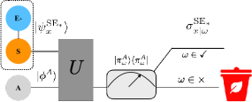
Figure 1: The post-selection of a system in mixed states can be artificially described as the post-selection on the join system consisting of the primary system and the optimal environment. The ancilla is introduced to implement the post-selection measurement.

Alternatively, we may prove Eq. (5) using the idea of purification. According to the Uhlman’s theorem [37, 4], $I[\rho(x)]\leq I(\ket{\psi^{\text{SE}}(x)})$, where $\ket{\psi^{\text{SE}}(x)}$ is a purification of $\rho(x)$ and the upper bound can be saturated by an optimal environment $E_{*}$. Thus, we consider the purification via the optimal environment $E_{*}$ and the post-selection channel $K_{\omega}\otimes\mathbb{I}^{\text{E}*}$, see Fig.  1. Applying Eq. (4) for the composite system consisting of the system, the optimal environment, and the ancilla, we obtain

$$I_{\omega}^{Q}[\sigma^{\text{SE}_{*}\text{A}}(x)]\leq I_{\omega}^{Q}[\ket{\psi^{\text{SE}_{*}}(x)}],$$ (7)

where

$$I_{\omega}^{Q}[\sigma^{\text{SE}_{*}\text{A}}(x)]=I_{\text{{\hbox{\omega}}}}^{\text{cl}}[p(\omega\big{|}x)]+p(\omega\big{|}x)I^{Q}[\ket{\psi^{\text{SE}_{*}}(x|\omega)}]$$ (8)

and $p(\omega\big{|}x)=\text{Tr}\left(\rho^{\text{SE}_{*}}(x)E_{\omega}\otimes\mathbb{I}^{\text{E}*}\right)=\text{Tr}\left(\rho(x)E_{\omega}\right)$, $\ket{\psi^{\text{SE}_{*}}(x|\omega)}=M_{\omega}\otimes\mathbb{I}^{\text{E}*}\ket{\psi^{\text{SE}_{*}}(x)}/\sqrt{p(\omega\big{|}x)}$ and $I_{\omega}^{Q}[\ket{\psi^{\text{SE}_{*}}(x)}]=4\braket{\partial_{x}^{\perp}\psi^{\text{SE}_{*}}(x)\big{missing}}{E_{\omega}\otimes\mathbb{I}^{\text{E}*}\big{missing}}{\partial_{x}^{\perp}\psi^{\text{SE}_{*}}(x)}$. Using the Uhlmann’s theorem once again, we know

$$I^{Q}[\ket{\psi^{\text{SE}_{*}}(x|\omega)}]\geq I_{\omega}^{Q}[\sigma(x|\omega)],$$ (9)

where $\sigma(x|\omega)=\text{Tr}_{\text{E}_{*}}\left(\ket{\psi^{\text{SE}_{*}}(x|\omega)}\bra{\psi^{\text{SE}_{*}}(x|\omega)}\right)$. This leads to a similar version of Eq. (4), i.e.,

$$I_{\omega}^{Q}[\sigma^{\text{S}\text{A}}(x)]\leq I_{\omega}^{Q}[\ket{\psi^{\text{SE}_{*}}(x)}]$$ (10)

Summing over both sides over $\omega$, we know

$$I^{Q}[\sigma^{\text{SA}}(x)]\leq I^{Q}[\ket{\psi^{\text{SE}_{*}}(x)}]\equiv I^{Q}[\rho(x)]$$ (11)

Now let us come to question (b). From above derivation, the saturation of Eq. (5) requires, in addition to saturation of a series of hierarchy of inequalities, the exact knowledge of the optimal environment $E_{*}$, which in general is formidable to find [5]. We may have the impression that post-selecting generic mixed states may likely lead to losses. Nevertheless, one could still ask (c): Are there mixed quantum states with particular features or structures such that they can be post-selected without loss?

The physics of lossless post-selection.— We would like to approach question (c) through a physics perspective, rather than overcoming the technical challenge of evaluating the QFI for mixed states. To this end, let us first revisit the post-selection of pure states discussed in Ref. [30]. For the sake of simplicity, at the moment, we shall focus on binary post-selection, where $\Omega=\{\checkmark,\,\times\}$. In this case, post-selection POVM can be chosen to be

$$E_{\checkmark}=\ket{\psi^{\perp}(x)}\bra{\psi^{\perp}(x)}+\lambda_{\checkmark}\ket{\psi(x)}\bra{\psi(x)},\lambda_{\checkmark}\in(0,1)$$ (12)

The post-selection measurement operator can be taken as

$$M_{\checkmark}=U_{\checkmark}\sqrt{E_{\checkmark}}=\ket{\psi^{\perp}(x)}\bra{\psi^{\perp}(x)}+\sqrt{\lambda_{\checkmark}}\ket{\psi(x)}\bra{\psi(x)}.$$ (13)

where $U_{\checkmark}$ is some unitary operator independent of $x$. Upon taking $U_{\checkmark}=\mathbb{I}$, it can be calculated in Ref.[30] that $\ket{\psi(x|\checkmark)}=\ket{\psi(x)}$ and

$$\partial_{x}\ket{\psi(x|\checkmark)}=\frac{1}{\sqrt{\lambda_{\checkmark}}}\ket{\partial_{x}\psi(x)}+\left(\frac{1}{\sqrt{\lambda_{\checkmark}}}-1\right)\braket{\psi(x)}{\partial_{x}\psi(x)}$$ (14)

Clearly, one can grasp qualitatively on the amplification mechanism of the post-selected QFI: The smaller the success probability is, the larger the prefactor $1/\sqrt{\lambda_{\checkmark}}$ on the first term of the r.h.s of Eq. (14) becomes. Here, we emphasize such an intuition is not quantitative as the role of the second term on the r.h.s. of Eq. (14) is not clear. Furthermore, such an intuition does not generalize to mixed states.

However, in terms of the density operator, we observe that

$$\rho(x|\checkmark)=\rho(x),\;\partial_{x}\rho(x|\checkmark)=\frac{1}{\sqrt{\lambda_{\checkmark}}}\partial_{x}\rho(x).$$ (15)

Eq. (15) is our first main result, which unveils the physics of the lossless post-selection measurement, as we now elaborate. According to Eq. (6), Eq. (15) immediately implies

$$L(x|\checkmark)=\frac{1}{\sqrt{\lambda_{\checkmark}}}L(x),$$ (16)

where $L(x|\checkmark)$ and $L(x)$ are the SLDs for $\rho(x|\checkmark)$ and $\rho(x)$, respectively. It follows from the generic definition of QFI, i.e., $I^{Q}[\rho(x)]=\text{Tr}[\rho(x)L^{2}(x)]$ [35] that

$$I^{Q}[\rho(x|\checkmark)]=\frac{1}{\lambda_{\checkmark}}I^{Q}[\rho(x)].$$ (17)

Here, one can clearly see that the intuition responsible for the amplification effect of the post-selected QFI is due to the amplification of the SLD. The lossless nature of the post-selection measurement follows from Eq. (17).

Finally, let us introduce some notations before turning to the post-selection of mixed states. We partition the Hilbert space to $\mathcal{H}=\mathcal{H}_{k}+\mathcal{H}_{r}$, where $\mathcal{H}_{k}$ and $\mathcal{H}_{r}$ are the kernel and the support of $\rho(x)$, respectively. $\mathcal{H}_{k}$ can be further decomposed as $\mathcal{H}_{k}=\mathcal{H}_{s}\oplus\mathcal{H}_{s}^{\perp}$, where $\mathcal{H}_{s}=\text{span}\{\Pi_{k}\ket{\partial_{x}\psi_{n}(x)}=\ket{\partial_{x}\psi_{n}(x)}-\Pi_{r}\ket{\partial_{x}\psi_{n}(x)}\}_{n=1}^{d_{\rho(x)}}\subseteq\mathcal{H}_{s}$, where $\Pi_{k}$ and $\Pi_{r}$ are the projects to the kernel $\mathcal{H}_{k}$ and the support $\mathcal{H}_{r}$ , respectively. As Eq. (15) is responsible for the amplification effect and lossless nature, we shall promote it to the level that it should also hold for mixed state post-selection. This leads to the following ansatz of the lossless post-selection measurement for mixed states, as a natural generalization of Eq. (12),

$$E_{\checkmark}=\Pi_{s}+\lambda_{\checkmark}\Pi_{r},\,\lambda_{\checkmark}\in(0,1)$$ (18)

where $\Pi_{s}$ and $\Pi_{r}$ are the projectors to the subspace $\mathcal{H}_{s}$ of the kernel and $\mathcal{H}_{r}$, respectively. Here the subscripts $s$ and $r$ indicate the singular and regular projectors in the sense that $\text{Tr}[\Pi_{s}\rho(x)]=0$ and $\text{Tr}[\Pi_{r}\rho(x)]\neq 0$, respectively [34]. It is straightforward to calculate that the first equation of Eq. (15) is satisfied immediately while the second equation of Eq. (15) leads to

$$\Pi_{r}\partial_{x}\rho(x)\Pi_{r}=\Pi_{r}L(x)\Pi_{r}=0.$$ (19)

Furthermore, it can be easily shown that [38] that $\Pi_{s}\partial_{x}\rho(x)\Pi_{s}=0$ is an identity, which holds for all density operators. On the other hand, the value of SLD on $\mathcal{H}_{k}$ is ambiguous, as it is always consistent with the definition (6). Here we shall choose the one that vanishes on $\mathcal{H}_{k}$. Therefore, we conclude our second main result: Eq. (18) is lossless if $\partial_{x}\rho(x)$ or the SLD $L(x)$ bears the “block off-diagonal structure”, i.e., it vanishes on both the support and kernel of $\rho(x)$.

Consider any convex decomposition $\rho(x)=\sum_{n=1}^{N}p_{n}(x)\ket{\psi_{n}(x)}\bra{\psi_{n}(x)}$, where $p_{n}(x)$ is strictly positive and $\{\ket{\psi_{n}(x)}\}$ is a set of normal, but not necessarily orthogonal bases, and $N\geq d_{\rho(x)}=\text{rank}[\rho(x)]$, [39]. Since $\{\ket{\psi_{n}(x)}\}$ spans $\mathcal{H}_{r}$, Eq. (19) is equivalent as [38]

$$\braket{\psi_{k}(x)}{\partial_{x}\rho(x)}{\psi_{l}(x)}=0,\forall k,l$$ (20)

In the special case of spectral decomposition, $\braket{\psi_{k}(x)}{\partial_{x}\rho(x)}{\psi_{l}(x)}$ becomes $\partial_{x}p_{k}(x)\delta_{kl}+\Delta p_{kl}(x)\braket{\partial_{x}\psi_{k}(x)}{\psi_{l}(x)}$, where $\Delta p_{kl}(x)=p_{k}(x)-p_{l}(x)$.

A few comments: (i) For a pure state, in the basis of $\ket{\psi(x)}$ and $\ket{\psi^{\perp}(x)}$, $\partial_{x}\rho(x)=\begin{bmatrix}0&1\\ 1&0\end{bmatrix}$, which obviously satisfy Eq. (19). (ii) Similar with the pure states case, it is possible to deform Eq. (18) into post-selection measurements with multiple outcomes, $E_{\omega}=q_{\omega}\Pi_{s}+\lambda_{\omega}\Pi_{r}$, where $\lambda_{\omega}\in(0,1)$, $\omega\in\checkmark$ and $\sum_{\omega\in\checkmark}q_{\omega}=1$. A redundant projector onto the subspace $\mathcal{H}_{s}^{\perp}$ can be also added to $E_{\omega}$ as in the case of pure states, which does influence its optimality. In general, for $\omega\in\checkmark$, $M_{\omega}=U_{\omega}\sqrt{E}_{\omega}$, where $U_{\omega}$ is some unitary operator that may varies between different outcomes. (iii) It is important to note that in order for the lossless post-selection (18), $\rho(x)$ must be rank-deficient. In the case where $\rho(x)$ is full-rank, ancillas must be supplied to enlarge the Hilbert space. (iv) Finally, when applying to concrete examples, any convex combination of Eq. (19) can work. There is no need to diagonalize $\rho(x)$.

Examples. — Now we apply our theory to practical quantum metrological problems. To characterize the performance of the lossless post-selection measurement (18), we take $M_{\checkmark}=\sqrt{E_{\checkmark}}$ and define the figure of merits

$$\varepsilon_{0}(x)\equiv\|\rho(x|\checkmark)-\rho(x)\|,\,\varepsilon_{1}(x)\equiv\|\partial_{x}\rho(x|\checkmark)-\partial_{x}\rho(x)/\sqrt{\lambda_{\checkmark}}\|,$$ (21)

where $\|\cdot\|$ denotes some operator norm.

As a first example, we consider the superresolution imaging of two point sources with a Gaussian point-spread function [40], which is described by the following rank$-2$ state

$$\rho(x)=q\ket{\psi_{+}(x)}\bra{\psi_{+}(x)}+(1-q)\ket{\psi_{-}(x)}\bra{\psi_{-}(x)}$$ (22)

where $\ket{\psi_{\pm}(x)}=e^{-i\hat{P}\left(\pm\frac{x}{2}\right)}\ket{\psi_{0}}$, $\braket{u}{\psi_{0}}=\left(\frac{1}{2\pi\sigma^{2}}\right)^{1/4}e^{-\frac{u^{2}}{4\sigma^{2}}}$ and $\hat{P}$ is the momentum operator defined as $\braket{u}{\hat{P}}{\psi}=-\text{i}\partial_{u}\braket{u}{\psi}$ . Since we focus on single-parameter estimation and study the fundamental limits of post-selection, we assume the intensities of the sources are known. In this case, it can shown that $I^{Q}[\rho(x)]=1/(4\sigma^{2})$, independent of the values of the source intensities and the values of $x$ [42, 43].

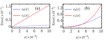
Figure 2: The errors of the post-selection measurements Eq. (18) and Eq. (25) for (a) superresolution and (b) two-qubit example in the limit $x\to 0$, respectively. The norms used in the numerical calculation of Eq. (21) are the $L^{2}$-norm and matrix-$2$ norm for (a) and (b), respectively. Values of parameters: (a) $\lambda=10^{-2}$, $\sigma=1$, $q=0.3$. (b)$\lambda=10^{-4}$, $q=0.3$.

Note that Eq. (22) is a convex decomposition, but not the spectral decomposition. It can be readily observed that in the Rayleigh limit $x\to 0$, Eq. (20) is satisfied. Intuitively, this can be seen as follows: When $x\to 0$, both $\mathcal{H}_{s}$ and $\mathcal{H}_{r}$ become the rank$-1$ subspaces with bases $\ket{\psi_{1}}$ and $\ket{\psi_{0}}$, respectively, where $\langle u|\psi_{1}\rangle=u\braket{u}{\psi_{0}}/\sigma$ is the first-order Hermite-Gaussian function. It follows that $\lim_{x\to 0}\braket{\psi_{0}}{\partial_{x}\rho_{x}}{\psi_{0}}=0$. More precisely, one can calculate that for all values of $x$,

$$\braket{\psi_{+}(x)}{\partial_{x}\rho(x)}{\psi_{+}(x)} =2q\text{i}\langle\hat{P}e^{-\text{i}\hat{P}x}\rangle\langle e^{\text{i}\hat{P}x}\rangle,$$

$$\braket{\psi_{-}(x)}{\partial_{x}\rho(x)}{\psi_{-}(x)} =2(1-q)\text{i}\langle\hat{P}e^{-\text{i}\hat{P}x}\rangle\langle e^{\text{i}\hat{P}x}\rangle,$$

$$\braket{\psi_{+}(x)}{\partial_{x}\rho(x)}{\psi_{-}(x)} =\text{i}\langle\hat{P}e^{-\text{i}\hat{P}x}\rangle,$$

where the average is taken over the state $\ket{\psi_{0}}$. It is clear that Eq. (20) is satisfied in the limit $x\to 0$ thanks to $\langle\hat{P}\rangle=0$.

Therefore, in the Rayleigh limit, we can approximately use the post-selection measurement

$$E_{\checkmark}=\ket{\psi_{1}}\bra{\psi_{1}}+\lambda_{\checkmark}\ket{\psi_{0}}\bra{\psi_{0}}$$ (23)

to reduce the number of detected photons. The performance of this Eq. (23) is shown in Fig. 2(a). Under the $L^{2}$-norm defined as $\|f\|=\sqrt{\int_{-\infty}^{\infty}|f(u,u^{\prime})|^{2}dudu^{\prime}}$, it can be analytically calculated straightforwardly that to the leading order of $x$, $\varepsilon_{0}(x)=|2q-1|(1-\sqrt{\lambda})x/(2\sqrt{2}\sqrt{\lambda}\sigma)$ and $\varepsilon_{1}(x)=\sqrt{2-4\sqrt{\lambda}+3\lambda}x/(8\lambda\sigma^{2})$.

It is straightforward to generalize the arguments here to the case of Zernike point spread function [34] or the estimation of the longitudinal separation  [44]. More interestingly, post-selection measurement of this type has also been shown to be the lossless post-selection channel in the von Neumann measurement model for estimating the spin-meter coupling strength [30].

Next, we consider mixed states generated through unitary dynamic encoding, i.e. $\rho(x)=U(x)\rho_{0}U^{\dagger}(x)$. Denoting the spectral decomposition of $\rho_{0}$ as $\rho_{0}=\sum_{n}q_{n}\ket{\phi_{n}}\bra{\phi_{n}}$, where $q_{n}>0$, we find Eq. (20) reduces to

$$\Delta q_{kl}\langle\phi_{k}|H(x)|\phi_{l}\rangle=0,\,\forall k\neq l,$$ (24)

where $H(x)=\text{i}\partial_{x}U^{\dagger}(x)U(x)$. Given any distinct pair of $k,l$, we know at least one the following conditions $q_{k}=q_{l}$ or $\langle\phi_{k}|H(x)|\phi_{l}\rangle$ must hold. In this case, the QFI takes a simple form [36]:

$$I^{Q}[\rho(x)]=4\left[\sum_{k}q_{k}\text{Var}[H(x)]_{\ket{\phi_{k}}}\!-\!\sum_{k,l,\,l\neq k,q_{l}=q_{k}}q_{k}|\langle\phi_{k}|H(x)|\phi_{l}\rangle|^{2}\right]$$

More specifically, we can consider quantum metrology with two-qubit unitary $U(x)=e^{-\text{i}\sigma_{x}^{(1)}\sigma_{x}^{(2)}x}$. The optimal pure initial state for estimating $x$ can be $\ket{\phi_{1}}=\ket{00}$ and $\ket{\phi_{2}}=\ket{01}$. Suppose there is uncertainty in preparing the second qubit in the computation basis so that the initial state becomes mixed, i.e. $\rho_{0}=q\ket{\phi_{1}}\bra{\phi_{1}}+(1-q)\ket{\phi_{2}}\bra{\phi_{2}}$. It is straightforward to check $\braket{\phi_{1}}{\sigma_{x}^{(1)}\sigma_{x}^{(2)}}{\phi_{2}}=0$ and therefore $I^{Q}[\rho(x)]=I^{Q}[\ket{\psi_{1}(x)}]=I^{Q}[\ket{\psi_{2}(x)}]=4$, where $\ket{\psi_{n}(x)}=U(x)\ket{\phi_{n}}$. In ultra-sensitive estimation where $x$ is very close zero, it can be readily found that $\mathcal{H}_{k}=\text{span}\{\ket{11},\,\ket{10}\}$ and $\mathcal{H}_{r}=\text{span}\{\ket{00},\ket{01}\}$. Then

$$E_{\checkmark}=\ket{1^{(1)}}\bra{1^{(1)}}+\lambda_{\checkmark}\ket{0^{(1)}}\bra{0^{(1)}}$$ (25)

becomes the post-selection measurement only on the first qubit, reminiscent of the weak value amplification. The performance of Eq. (25) is shown in Fig. 2(b).

Discussion and conclusion. — While the amplification effect on the precision due to post-selection seems counterintuitive and confusing, here through a typical two-outcome post-selection channel, we give a straightforward intuition on the amplification effect: Up to a parameter-independent unitary operation, post-selection amplifies the parametric derivative of the density operator while preserving the original state. Based on this intuition, we give the first construction of the loss post-selection measurement on mixed states when the parametric derivative of the density operator or the SLD operator possesses the so-called “block off-diagonal structure”. Our results provide a foundation for post-selected quantum metrology in noisy environments. In the future, it may be interesting to furthermore explore the suppression technical noise [45] of the estimating of mixed states through post-selection measurement.

On the fundamental side, despite the state being mixed, interestingly the “block off-diagonal structure” implies that the state behaves like a pure state. This observation may provide insights into many other problems concerning mixed states in quantum information theory, including the tightness of quantum speed limits for mixed states [46, 47, 48], the construction of optimal measurements when a mixed state satisfies the partial commutativity condition [34, 49].

Acknowledgement. — It is a pleasure to acknowledge inspiring discussions with David Arvidsson-Shukur, Luiz Davidovich, Wenchao Ge, Liang Jiang, Andrew Jordan, Spencer Rogers, and Luis Sanchez-Soto, as well as the hospitality of the Institute of Quantum Studies at Chapman University, the Pritzker School of Molecular Engineering at the University of Chicago, and the Department of Physics at the University of Rhode of Island. This work was supported by the Wallenberg Initiative on Networks and Quantum Information (WINQ) program.

Supplemental Material

I Proof of Eq. (19)

We take the post-selection measurement channel as

$$M_{\checkmark}=\sqrt{E_{\checkmark}}=\Pi_{s}+\sqrt{\lambda}_{\checkmark}\Pi_{r}.$$ (S1)

The post-selected state is

$$\rho(x|\checkmark)=\frac{M_{\checkmark}\rho_{x}M_{\checkmark}^{\dagger}}{\text{Tr}\left[M_{\checkmark}\rho_{x}M_{\checkmark}^{\dagger}\right]},$$ (S2)

Therefore

$$\partial_{x}\rho(x|\checkmark)=\frac{M_{\checkmark}\partial_{x}\rho(x)M_{\checkmark}^{\dagger}}{\lambda_{\checkmark}}-\frac{M_{\checkmark}\rho(x)M_{\checkmark}^{\dagger}}{\lambda_{\checkmark}^{2}}\text{Tr}\left[M_{\checkmark}\partial_{x}\rho_{x}M_{\checkmark}^{\dagger}\right].$$ (S3)

We first consider the spectral decomposition of $\rho(x)$

$$\rho(x)=\sum_{n=1}^{d_{\rho(x)}}q_{n}(x)\ket{\varphi_{n}(x)}\bra{\varphi_{n}(x)}$$

It is also straightforward to calculate

$$\partial_{x}\rho(x)=\sum_{n=1}^{d_{\rho(x)}}\partial_{x}q_{n}(x)\ket{\varphi_{n}(x)}\bra{\varphi_{n}(x)}+\sum_{n=1}^{d_{\rho(x)}}p_{n}(x)\ket{\partial_{x}\varphi_{n}(x)}\bra{\varphi_{n}(x)}+\sum_{n=1}^{d_{\rho(x)}}\partial_{x}p_{n}(x)\ket{\varphi_{n}(x)}\bra{\partial_{x}\varphi_{n}(x)}.$$ (S4)

We denote the remaining normal basis orthogonal to $\{\ket{\varphi_{n}(x)}\}$ as $\ket{e_{m}(x)}$. Clearly,

$$\Pi_{s}=\sum_{m}\ket{e_{m}(x)}\bra{e_{m}(x)},\>\Pi_{r}=\sum_{n=1}^{d_{\rho(x)}}\ket{\varphi_{n}(x)}\bra{\varphi_{n}(x)}.$$ (S5)

With Eq. (S4), it is straightforward to see

$$\Pi_{s}\partial_{x}\rho(x)\Pi_{s}=0$$ (S6)

holds for all density operators $\rho(x)$. Furthermore, it can be readily checked that

$$\text{Tr}[E_{\checkmark}\partial_{x}\rho(x)]=0,$$ (S7)

where $E_{\checkmark}$is defined in Eq. (18) in the main text. Given above facts, Eq. (S3) becomes

$$\partial_{x}\rho(x|\checkmark)=\frac{1}{\sqrt{\lambda_{\checkmark}}}[\Pi_{s}\partial_{x}\rho(x)\Pi_{r}+\text{h.c.}]+\Pi_{r}\partial_{x}\rho(x)\Pi_{r}.$$ (S8)

Now imposing Eq. (15) in the main text, we obtain

$$\Pi_{s}\partial_{x}\rho(x)\Pi_{r}+\text{h.c.}+\Pi_{r}\partial_{x}\rho(x)\Pi_{r}+\sqrt{\lambda_{\checkmark}}\Pi_{r}\partial_{x}\rho(x)\Pi_{r}=\partial_{x}\rho(x),$$ (S9)

which is reduce to, upon decomposing the r.h.s onto the partition $\mathcal{H}=\mathcal{H}_{r}+\mathcal{H}_{s}$,

$$\left(1-\sqrt{\lambda_{\checkmark}}\right)\Pi_{r}\partial_{x}\rho(x)\Pi_{r}=0.$$ (S10)

Since we exclude the trivial case where $\lambda_{\checkmark}$ (corresponding to applying identity post-selection measurements), we end up with

$$\Pi_{r}\partial_{x}\rho(x)\Pi_{r}=0$$ (S11)

Eq. (19) is equivalent to

$$\braket{\varphi_{k}(x)}{\partial_{x}\rho(x)}{\varphi_{l}(x)}=0,\,\forall k,\,l=1,2,\cdots d_{\rho(x)}.$$ (S12)

Using the definition of the SLD (6), we find

$$\braket{\varphi_{k}(x)}{\partial_{x}\rho(x)}{\varphi_{l}(x)}=[p_{k}(x)+p_{l}(x)]\braket{\varphi_{k}(x)}{L(x)}{\varphi_{l}(x)}=0$$ (S13)

Since $p_{k}(x)$ and $p_{l}(x)$ are strictly positive, we conclude that Eq. (S11) also implies

$$\braket{\varphi_{k}(x)}{L(x)}{\varphi_{l}(x)}=0,\,\forall k,\,l=1,2,\cdots d_{\rho(x)}.$$ (S14)

which concludes the proof of Eq. (19) in the main text.

II Proof of Eq. (20)

For a convex decomposition

$$\rho(x)=\sum_{n=1}^{N}p_{n}(x)\ket{\psi_{n}(x)}\bra{\psi_{n}(x)},$$

since $\ket{\psi_{n}(x)}$ must be a linear combination of the set of the orthonormal of basis $\{\varphi_{k}(x)\}_{k=1}^{d_{\rho(x)}}$, Eq. (S12) implies Eq. (20) in the main text. On the other hand, using the Gram-Schmidt orthogonalization process, it is straightforward to see that Eq. (20) implies Eq. (19)

Furthermore, in the spectral representation of $\rho(x)$, it is straightforward to calculate

$$\braket{\varphi_{k}(x)}{\partial_{x}\rho(x)}{\varphi_{l}(x)} =\partial_{x}p_{k}(x)\delta_{kl}+p_{k}(x)\braket{\partial_{x}\varphi_{k}(x)}{\varphi_{l}(x)}+p_{l}(x)\braket{\varphi_{k}(x)}{\partial_{x}\varphi_{l}(x)}$$

$$=\partial_{x}p_{k}(x)\delta_{kl}+\Delta p_{kl}(x)\braket{\partial_{x}\varphi_{k}(x)}{\varphi_{l}(x)}+p_{l}(x)\left[\braket{\partial_{x}\varphi_{k}(x)}{\varphi_{l}(x)}+\braket{\varphi_{k}(x)}{\partial_{x}\varphi_{l}(x)}\right]$$

$$=\partial_{x}p_{k}(x)\delta_{kl}+\Delta p_{kl}(x)\braket{\partial_{x}\varphi_{k}(x)}{\varphi_{l}(x)},$$ (S15)

where in the last step we have used the fact that $\braket{\varphi_{k}(x)}{\varphi_{l}(x)}=0$.

References

- Helstrom [1976] C. W. Helstrom, Quantum Detection and Estimation Theory (Academic Press, 1976).
- Holevo [2011] A. S. Holevo, Probabilistic and Statistical Aspects of Quantum Theory (Springer Science & Business Media, 2011).
- Hayashi [2005] M. Hayashi, ed., Asymptotic Theory Of Quantum Statistical Inference: Selected Papers (World Scientific Pub Co Inc, Singpore, 2005).
- Escher et al. [2011] B. M. Escher, R. L. de Matos Filho, and L. Davidovich, Nature Physics 7, 406 (2011).
- Escher et al. [2012] B. M. Escher, L. Davidovich, N. Zagury, and R. L. De Matos Filho, Physical Review Letters 109, 190404 (2012).
- Chin et al. [2012] A. W. Chin, S. F. Huelga, and M. B. Plenio, Physical Review Letters 109, 233601 (2012).
- Demkowicz-Dobrzański et al. [2012] R. Demkowicz-Dobrzański, J. Kołodyński, and M. Guţă, Nature Communications 3, 1063 (2012).
- Alipour et al. [2014] S. Alipour, M. Mehboudi, and A. T. Rezakhani, Physical Review Letters 112, 120405 (2014).
- Demkowicz-Dobrzański and Maccone [2014] R. Demkowicz-Dobrzański and L. Maccone, Physical Review Letters 113, 250801 (2014).
- Alipour and Rezakhani [2015] S. Alipour and A. T. Rezakhani, Physical Review A 91, 042104 (2015).
- Smirne et al. [2016] A. Smirne, J. Kołodyński, S. F. Huelga, and R. Demkowicz-Dobrzański, Physical Review Letters 116, 120801 (2016).
- Beau and del Campo [2017] M. Beau and A. del Campo, Physical Review Letters 119, 010403 (2017).
- Demkowicz-Dobrzański et al. [2017] R. Demkowicz-Dobrzański, J. Czajkowski, and P. Sekatski, Physical Review X 7, 041009 (2017).
- Haase et al. [2018] J. F. Haase, A. Smirne, S. F. Huelga, J. Kołodynski, and R. Demkowicz-Dobrzanski, Quantum Measurements and Quantum Metrology 5, 13 (2018).
- Liu and Yuan [2017] J. Liu and H. Yuan, Physical Review A 96, 012117 (2017).
- Yang [2019] Y. Yang, Physical Review Letters 123, 110501 (2019).
- Altherr and Yang [2021] A. Altherr and Y. Yang, Physical Review Letters 127, 060501 (2021).
- Bai and An [2023] S.-Y. Bai and J.-H. An, Physical Review Letters 131, 050801 (2023).
- Yang [2024] J. Yang, “When does dissipative evolution preserve and amplify metrological information?” (2024), arxiv:2401.15622 [quant-ph] .
- Aharonov et al. [1988] Y. Aharonov, D. Z. Albert, and L. Vaidman, Physical Review Letters 60, 1351 (1988).
- Hosten and Kwiat [2008] O. Hosten and P. Kwiat, Science 319, 787 (2008).
- Dixon et al. [2009] P. B. Dixon, D. J. Starling, A. N. Jordan, and J. C. Howell, Physical Review Letters 102, 173601 (2009).
- Starling et al. [2009] D. J. Starling, P. B. Dixon, A. N. Jordan, and J. C. Howell, Physical Review A 80, 041803 (2009).
- Starling et al. [2010] D. J. Starling, P. B. Dixon, A. N. Jordan, and J. C. Howell, Physical Review A 82, 063822 (2010).
- Xu et al. [2013] X.-Y. Xu, Y. Kedem, K. Sun, L. Vaidman, C.-F. Li, and G.-C. Guo, Physical Review Letters 111, 033604 (2013).
- Dressel et al. [2014] J. Dressel, M. Malik, F. M. Miatto, A. N. Jordan, and R. W. Boyd, Reviews of Modern Physics 86, 307 (2014).
- Arvidsson-Shukur et al. [2020] D. R. M. Arvidsson-Shukur, N. Yunger Halpern, H. V. Lepage, A. A. Lasek, C. H. W. Barnes, and S. Lloyd, Nature Communications 11, 3775 (2020).
- Lupu-Gladstein et al. [2022] N. Lupu-Gladstein, Y. B. Yilmaz, D. R. M. Arvidsson-Shukur, A. Brodutch, A. O. T. Pang, A. M. Steinberg, and N. Y. Halpern, Physical Review Letters 128, 220504 (2022).
- Jenne and Arvidsson-Shukur [2022] J. H. Jenne and D. R. M. Arvidsson-Shukur, Physical Review A 106, 042404 (2022).
- Yang [2023] J. Yang, “Theory of Compression Channels for Post-selected Metrology,” (2023), arxiv:2311.06679 [quant-ph, stat] .
- Salvati et al. [2023] F. Salvati, W. Salmon, C. H. W. Barnes, and D. R. M. Arvidsson-Shukur, “Compression of metrological quantum information in the presence of noise,” (2023), arxiv:2307.08648 [quant-ph] .
- Combes et al. [2014] J. Combes, C. Ferrie, Z. Jiang, and C. M. Caves, Physical Review A 89, 052117 (2014).
- Braunstein and Caves [1994] S. L. Braunstein and C. M. Caves, Physical Review Letters 72, 3439 (1994).
- Yang et al. [2019] J. Yang, S. Pang, Y. Zhou, and A. N. Jordan, Physical Review A 100, 032104 (2019).
- Paris [2009] M. G. A. Paris, International Journal of Quantum Information 07, 125 (2009).
- Liu et al. [2019] J. Liu, H. Yuan, X.-M. Lu, and X. Wang, Journal of Physics A: Mathematical and Theoretical 53, 023001 (2019).
- Uhlmann [1976] A. Uhlmann, Reports on Mathematical Physics 9, 273 (1976).
- [38] See Supplemental Material.
- Fujiwara and Imai [2008] A. Fujiwara and H. Imai, Journal of Physics A: Mathematical and Theoretical 41, 255304 (2008).
- Tsang et al. [2016] M. Tsang, R. Nair, and X.-M. Lu, Physical Review X 6, 031033 (2016).
- Note [1] It should not be confused that here denotes the position while denotes the estimation parameter.
- Řehaček et al. [2017] J. Řehaček, Z. Hradil, B. Stoklasa, M. Paúr, J. Grover, A. Krzic, and L. L. Sánchez-Soto, Physical Review A 96, 062107 (2017).
- Řeháček et al. [2018] J. Řeháček, Z. Hradil, D. Koutný, J. Grover, A. Krzic, and L. L. Sánchez-Soto, Physical Review A 98, 012103 (2018).
- Zhou et al. [2019] Y. Zhou, J. Yang, J. D. Hassett, S. M. H. Rafsanjani, M. Mirhosseini, A. N. Vamivakas, A. N. Jordan, Z. Shi, and R. W. Boyd, Optica 6, 534 (2019).
- Jordan et al. [2014] A. N. Jordan, J. Martínez-Rincón, and J. C. Howell, Physical Review X 4, 011031 (2014).
- Mandelstam and Tamm [1945] L. Mandelstam and Ig. Tamm, Journal of Physics-USSR 9, 249 (1945).
- Anandan and Aharonov [1990] J. Anandan and Y. Aharonov, Physical Review Letters 65, 1697 (1990).
- del Campo et al. [2013] A. del Campo, I. L. Egusquiza, M. B. Plenio, and S. F. Huelga, Physical Review Letters 110, 050403 (2013).
- Horodecki et al. [2022] P. Horodecki, Ł. Rudnicki, and K. Życzkowski, PRX Quantum 3, 010101 (2022).