Chapter 16 Posterior exploration for computationally intensive forward models
Mikkel B. Lykkegaard, Colin Fox, Dave Higdon, C. Shane Reese,
and J. David Moulton
To appear in the Handbook of Markov Chain Monte Carlo (2nd edition),
probably as Chapter 16.
1 Introduction
In a common inverse problem, we wish to infer about an unknown spatial field given indirect observations . The observations, or data, are linked to the unknown field through some physical system
where denotes the actual physical system and is an -vector of observation errors. Examples of such problems include medical imaging (Kaipio and Somersalo,, 2004), geologic and hydrologic inversion (Stenerud et al.,, 2008), and cosmology (Jimenez et al.,, 2004). When a forward model, or simulator , is available to model the physical process, one can model the data using the simulator
where includes observation error as well as error due to the fact that the simulator may be systematically different from reality for input condition . Our goal is to use the observed data to make inference about the spatial input parameters – predict and characterize the uncertainty in the prediction for .
The likelihood is then specified to account for both mismatch and sampling error. We will assume zero-mean Gaussian errors so that
| (1.1) |
with known. It is worth noting that the data often come from only a single experiment. So while it is possible to quantify numerical errors, such as those due to discretization (e.g.,Kaipio and Somersalo, (2004); Nissinen et al., (2008)), there is no opportunity to obtain data from additional experiments for which some controllable inputs have been varied. Because of this limitation, there is little hope of determining the sources of error in due to model inadequacy. Therefore, the likelihood specification will often need to be done with some care, incorporating the modeler’s judgment about the appropriate size and nature of the mismatch term.
In many inverse problems we wish to reconstruct , an unknown process over a regular 2-d lattice. We consider systems for which the model input parameters denote a spatial field or image. The spatial prior is specified for , which typically takes into account modeling, and possibly computational considerations.
The resulting posterior is then given by
This posterior can, in principle, be explored via Markov chain Monte Carlo (MCMC). However the combined effects of the high dimensionality of and the computational demands of the simulator make implementation difficult, and often impossible, in practice. By itself, the high dimensionality of isn’t necessarily a problem. MCMC has been carried out with relative ease in large image applications (Weir,, 1997; Rue,, 2001). However, in these examples, the forward model was either trivial, or non-existent. Unfortunately, even a mildly demanding forward simulation model can greatly affect the feasibility of doing MCMC to solve the inverse problem.
In this chapter we apply a standard single-site updating scheme that dates back to Metropolis et al., (1953) to sample from this posterior. While this approach has proven effective in a variety of applications, it has the drawback of requiring millions of calls to the simulation model. In Section 3 we consider an MCMC scheme that uses highly multivariate updates to sample from : the multivariate random walk Metropolis algorithm (Gelman et al.,, 1996). Such multivariate updating schemes are alluring for computationally demanding inverse problems since they have the potential to update many (or all) components of at once, while requiring only a single evaluation of the simulator.
Next, in Section 4, we consider augmenting the basic posterior formulation with additional formulations based on faster, approximate simulators. We create two faster, approximate forward models: by leveraging an incomplete multigrid solve; and by coarsening the initial “fine-scale” formulation described in the next section. These approximate simulators can be used in a delayed acceptance scheme (Liu,, 2001; Christen and Fox,, 2005), as well as in an augmented formulation (Higdon et al.,, 2002). Both of these recipes can be utilized with any of the above MCMC schemes, often leading to substantial improvements in efficiency. For a given , resulting output produced by the approximate multigrid model is quite close to that obtained by exact solve of the fine scale model . However, the coarser model shows substantial, systematic differences from the output of the fine-scale model . So we also consider the stochastic approaches for correcting systematic errors between the coarse- and fine-scale model output, introduced in Cui et al., (2011). We find that the corrected coarse model enables cheap and semi-automatic generation of multivariate proposals from the single-site proposal, with an appreciable acceptance rate in the fine-scale chain, giving improved efficiency.
The updating schemes are illustrated with an electrical impedance tomography (EIT) application described in the next section, where the values of denote electrical conductivity of a 2-d object. The chapter concludes with a discussion and some general recommendations.
2 An inverse problem in electrical impedance tomography
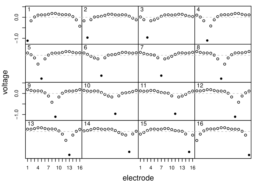
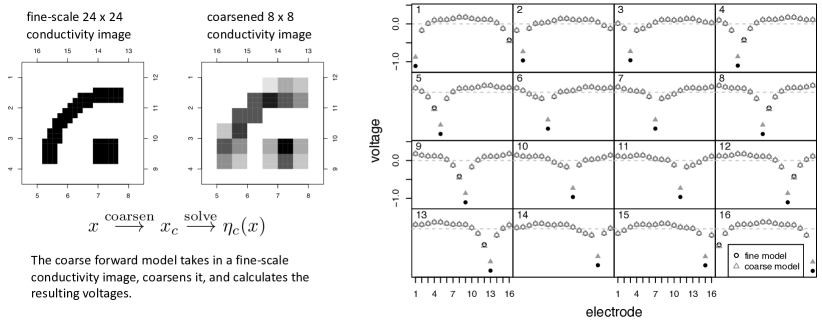
Bayesian methods for EIT applications have been described in Fox and Nicholls, (1997), Kaipio et al., (2000) and Andersen et al., (2003). A notional inverse problem is depicted in Figure 16.1; this setup was given previously in Moulton et al., (2008). Here a 2-d object composed of regions with differing electrical conductivity is interrogated by electrodes. From each electrode, in turn, a current is injected into the object and taken out at a rate of at the remaining 15 electrodes. The voltage is then measured at each of the 16 electrodes. These 16 experimental configurations result in voltage observations which are denoted by the -vector . The measurement error is simulated by adding iid mean 0 Gaussian noise to each of the voltage measurements. The standard deviation of this noise is chosen so that the signal to noise ratio is about 1000:3, which is typical of actual EIT measurements. The resulting simulated data is shown in the right frame of Figure 16.1 – one plot for each of the 16 circuit configurations. In each of those plots, the injector electrode is denoted by the black plotting symbol.

We take to denote spatial locations within the object , and take to denote the electrical conductivity at site . We also take to be the potential at location , and to be the current at boundary location . A mathematical model for the measurements is then the Neumann boundary-value problem
where denotes the boundary of the object and is the unit normal vector at the boundary location . The conservation of current requires that the sum of the currents at each of the 16 electrodes be 0. The arbitrary additive offset in the solution of this Neumann problem is determined by requiring that the sum of voltages at boundary electrodes is zero.
In order to numerically solve this problem for a given set of currents at the electrodes and a given conductivity field, , the conductivity field is discretized into an lattice. We use a standard Cholesky-based sparse solver for this system. Later in Section 4, we also create a faster, approximate solver based on an discretization of the conductivity field.
Now, for any specified conductivity configuration and current configuration, the solver produces 16 voltages. For all 16 current configurations, the forward solver produces an -vector of resulting voltages . Hence the sampling model for the data given the conductivity field is given by (1.1) where .
For the conductivity image prior, we adapt a Markov random field (MRF) prior from Geman and McClure, (1987). This prior has the form
| (2.1) |
where and control the regularity of the field, and is the tricube function of Cleveland, (1979)
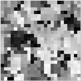
The sum is over all horizontal and vertical nearest neighbors denoted by and given by the edges in the Markov random field graph in Figure 16.2. Hence this prior encourages neighboring ’s to have similar values, but once and are more than apart, the penalty does not grow. This allows occasional large shifts between neighboring ’s. For this chapter, we fix . A realization from this prior is shown in the right frame of Figure 16.2. A typical prior realization shows patches of homogeneous values, along with abrupt changes in intensity at each patch boundary. This prior also allows an occasional, isolated, extreme single pixel value.
The resulting posterior density has the form
| (2.2) |
The patchiness and speckle allowed by this prior along with the rather global nature of the likelihood make posterior exploration for this inverse problem rather challenging, and a good test case for various MCMC schemes that have been developed over the years. We note that nature of the posterior can be dramatically altered by changing the prior specification for . This is discussed later in this section.
This chapter considers a number of MCMC approaches for sampling from this posterior distribution. We start at the beginning.
2.1 Posterior exploration via single-site Metropolis updates
A robust and straightforward method for computing samples from the posterior is the single-site Metropolis scheme, originally carried out in Metropolis et al., (1953) on the world’s first computer with addressable memory, the MANIAC. A common formulation of this scheme is summarized in Algorithm 1 using pseudo code.
This scheme is engineered to maintain balance with the posterior distribution – so that the nett movement between any two states and is done in proportion to the posterior density at these two points. The width of the proposal distribution should be adjusted so that inequality in line 7 is satisfied roughly half the time (Gelman et al.,, 1996), but an acceptance rate between 70% and 30% does nearly as well for single-site updates. The single-site Metropolis in Algorithm 1 scans through each of the parameter elements in a fixed, deterministic order (for loop, steps 3–9) to define one sweep over parameter values. One typically records the current value of after each sweep; we do so every 10 sweeps.
This single-site scheme was originally intended for distributions with very local dependencies within the elements of so that the ratio in line 6 simplifies dramatically. In general, this simplification depends on the full conditional density of
This density is determined by keeping all of the product terms in that contain , and ignoring the terms that don’t. Hence the ratio in line 7 can be rewritten as
In many cases this ratio becomes trivial to compute. However, in the case of this particular inverse problem, we must still evaluate the simulator to compute this ratio. This is exactly what makes the MCMC computation costly for this problem.
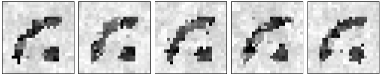
Nonetheless, this straightforward sampling approach does adequately sample the posterior, given sufficient computational effort; see Frigessi et al., (1993) for a proof of ergodicity. Figure 16.3 shows realizations produced by the single-site Metropolis algorithm, separated by sweeps. Inspection of these realizations makes it clear that posterior realizations yield a crisp distinction between the high and low conductivity regions, as was intended by the MRF prior for . Around the boundary of the high conductivity region there is a fair amount of uncertainty as to whether or not a given pixel has high or low conductivity.
Figure 16.4 shows the resulting posterior mean for and shows the history of three pixel values over the course of the single-site updating scheme. The sampler was run until forward simulations were carried out. An evenly spaced sample of 4,000 values for three of the pixels is shown in the right frame of Figure 16.4. Note that for the middle pixel (blue circle), the marginal posterior distribution is bimodal – some realizations have the conductivity value near 3, others near 4. Being able to move between these modes is crucial for a well mixing chain. Getting this pixel to move between modes is not simply a matter of getting that one pixel to move by itself; the movement of that pixel is accomplished by getting the entire image to move between local modes of the posterior.
This local multimodality is largely induced by our choice of prior. For example, if we alter the prior model in (2.1) so that
| (2.3) |
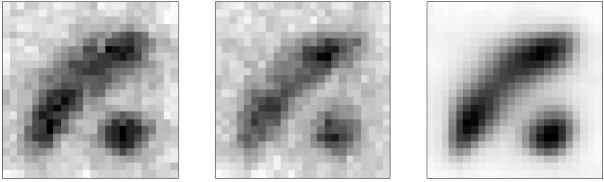
we have a standard Gaussian Markov random field (GMRF) prior for . If, in addition, the simulator is a linear mapping from inputs to ouputs , the resulting posterior is necessarily Gaussian, and hence, unimodal. While this is not true for nonlinear forward models/simulators, the GMRF prior still has substantial influence on the nature of the posterior; indeed, recent theoretical results show that the posterior for EIT with GMRF prior is typically log-concave (Nickl,, 2023), hence unimodal, confirming these computational observations. Figure 16.5 shows two realizations and the posterior mean resulting from such a prior with . Here posterior realizations are locally more variable – the difference between neighboring pixels are generally larger. However the global nature of the posterior realizations are far more controlled than those in Figure 16.3 since the GMRF prior suppresses local modes that appear under the previous formulation. This resulting formulation is also far easier to sample, requiring about a 10th of the effort needed for formulation in (2.2). An alternate, controlling prior formulation uses a process convolution prior for is given in the Appendix. In addition to yielding a more easily sampled posterior, the prior also represents the image with far fewer parameters than the used in the MRF specifications.
While these alternative specifications lead to simpler posterior distributions, they do so at the expense of overly smooth posterior realizations. Still, such realizations may be useful for exploratory purposes, and for initializing other samplers; we do not further pursue such formulations here. Instead, we focus on comparison of various MCMC schemes to sample the original gray level posterior in (2.2). We use the sample traces from the three pixels circled in Figure 16.4 to make comparisons between a variety of samplers which are discussed in the next sections – the movement of these three pixels is representative of all the image pixels. In particular, we focus on the frequency of movement between high and low conductivity at these sites.
3 Multivariate updating schemes
Schemes that propose to update more than just a single component of at a time have the potential to reduce the computational burden of producing an MCMC sample from . The single-site scheme above is also applicable when the proposal for changes some or all of the components of . However, producing a multivariate candidate that has an appreciable chance of being accepted (i.e., satisfying the inequality in line 7 of Algorithm 1) while allowing appreciable movement, is very difficult. This highlights a very appealing aspect of the single-site Metropolis scheme: even fairly thoughtless 1-d proposals have an appreciable chance of being accepted while adequately exploring the posterior.
There are clustering MCMC algorithms from statistical physics that allow for many pixels in to be updated at once (Edwards and Sokal,, 1988). Such methods can be adapted to this particular problem as in Higdon, (1998), however such methods typically show decreased efficiency relative to single-site updating when the likelihood is strong relative to the prior. This is certainly the case with our attempts on this application whose results are not worth discussing here. In the first edition of this handbook Higdon et al., (2011) we also explored the differential evolution-MCMC (DE-MCMC) sampler of ter Braak, (2006). However, we could not find an implementation that effectively sampled this EIT posterior so we do not further discuss DE-MCMC. Here we’ll consider some implementations of multivariate random walk Metropolis updating as competitors to the costly single-site Metropolis updating for our EIT application.
Later, in Section 4 we will also explore multivariate updates generated semi-automatically from the single-site Metropolis scheme by the MSDA algorithm, and highlight the adaptive MSDA algorithm that tunes a modified likelihood function to improve efficiency by leveraging an otherwise inadequate approximation to the forward map.
Random walk Metropolis
The multivariate random walk Metropolis (RWM) has been the focus of a number of theoretical investigations (Tierney,, 1994; Gelman et al.,, 1996). But to date this scheme has not been widely used in applications, and has proven advantageous only in simple, unimodal settings. The preference for single-site, or limited multivariate updates in practice may be attributed to how the full conditionals often simplify computation, or may be due to the difficulty in tuning highly multivariate proposals. In our EIT application, the univariate full conditionals do not lead to any computational advantages. If there is ever an application for which RWM may be preferable, this is it. Single-site updating is very costly, and may be inefficient relative to multivariate updating schemes for this multimodal posterior. The adaptive Metropolis (AM) method of Haario et al., (2006) automatically tunes a multivariate Gaussian proposal, and allows relatively automatic sampling for EIT with GMRF prior (Taghizadeh et al.,, 2020). However, we have not found that direct use of AM successfully samples in a complex inverse problem with multimodal posterior (see, e.g. Cui et al.,, 2011), such as the present posterior (2.2) that allows reconstruction of sharp conductivity boundaries in EIT.
A multivariate Gaussian random walk Metropolis scheme for
the -vector is summarized in Algorithm 2
using pseudo code.
We consider three different proposals for this scheme:
where is the posterior marginal sample variance for the conductivity , and is the sample covariance matrix – both estimated from the previously obtained single-site MCMC run. In each case we set where the scalar is chosen so that the candidate is accepted 30% of the time, which is close to optimal in a Gaussian setting.
MCMC traces for these three implementations of RWM are shown in Figure 16.6. The traces from the single-site Metropolis scheme are also given for comparison. Interestingly, the behavior of the traces varies with the choice of . The scheme with shows the most movement for the central pixel, which moves between high and low conductivity over the run. However its performance for the top, low conductivity pixel is noticeably worse. None of the RWM schemes do as well as single-site Metropolis when looking at the bottom, high conductivity pixel. These results suggest that a scheme that utilizes both single-site and RWM updates with might give slightly better posterior exploration than single-site Metropolis alone.
4 Augmenting with fast, approximate simulators
In many applications, a faster, approximate simulator is available for carrying out the forward model evaluation . There are a number of approaches for using fast, approximate simulators to improve the MCMC exploration of the original (fine-scale) posterior given in (2.2). In this chapter we consider two related approaches: Metropolis-coupled MCMC (Geyer,, 1991; Higdon et al.,, 2003; Andersen et al.,, 2003); and delayed acceptance (DA) schemes that limit the number of calls to the expensive, “exact” simulator (Liu,, 2001,Christen and Fox,, 2005,Cui et al.,, 2011,Banterle et al.,, 2019). We’ll also highlight the adaptive, multi-level extension of DA given in Lykkegaard et al., (2023), demonstrating it for the EIT application of this chapter.
We consider two different approximate forward models: 1) , based on an incomplete multigrid solve; and 2) , based on a coarsened representation of the conductivity image . The solver used for is derived from the BoxMG algorithm of Dendy, (1982) and is described in Higdon et al., (2011). Evaluating takes about a third of the time of evaluating the standard forward model . It calculates rather accurate voltages; all well within for each component of . In contrast, the coarse forward model is well over 100 times faster that , but far less accurate.
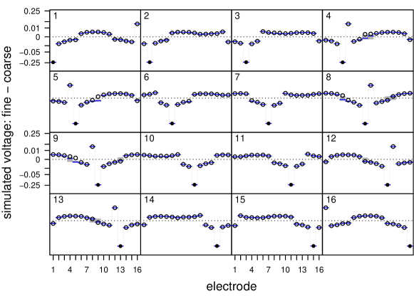
Its calculated voltages can be well over away from at the injector electrodes (see Figure 16.7). This error in poses problems for the basic implementations of Metropolis coupling and delayed acceptance described below, motivating an adaptive error implementation described in Section 4.3.
4.1 Metropolis coupling
By augmenting the posterior of interest with auxiliary distributions one can use Metropolis coupling (Geyer,, 1991), simulated tempering (Marinari and Parisi,, 1992), or related schemes (Liu and Sabatti,, 1999). Here we use Metropolis coupling (MC) and define a joint, product posterior for the pair of conductivity images given by
where the same priors are specified for and , and is the original likelihood, but with the multigrid forward model
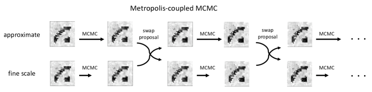
The posterior sampling proceeds by carrying out a fixed number of single site updates for and , using their respective posteriors, and then proposing a swap between and as shown in Figure 16.8. The swap from to is a deterministic Metropolis proposal, accepted with probability . Since can be evaluated in a third of the time required for , a parallel MC-MCMC implementation should allow three times the number of single-site Metropolis updates on the approximate posterior relative to the fine scale posterior before proposing a swap. This will approximately balance the load between the two processors carrying out the single site updates. Using the multigrid approximate forward model results in swaps that are accepted about 80% of the time, owing to its fidelity to the fine scale forward model. If the coarse forward model is used, swaps are never accepted due to its large error.
4.2 Delayed acceptance Metropolis
The delayed acceptance approach of Christen and Fox, (2005) uses a fast, approximate simulator to “filter” a proposal, similarly to the surrogate transition method of Liu, (2001), for dealing with complex forward models. For now, we define approximate posterior formulation using the multigrid simulator :
A simple Metropolis-based formulation of this scheme is given in Algorithm 3,
where and denote the posteriors using the exact and approximate simulators respectively. Notice that the exact simulator need only be run if the filtering condition () involving the faster, approximate simulator is satisfied. Hence, if the proposal width is chosen so that the filtering condition is satisfied only a third of the time, the exact simulator is only run for a third of the MCMC iterations. Using the multigrid simulator , the iterations required for our original single-site Metropolis scheme take about 66% of the computational effort using this delayed acceptance approach. Using the coarse simulator in this delayed acceptance algorithm is ineffective. Any proposal accepted in the approximate test (step 5, algorithm 3) is nearly always rejected in the fine scale test (step 6).
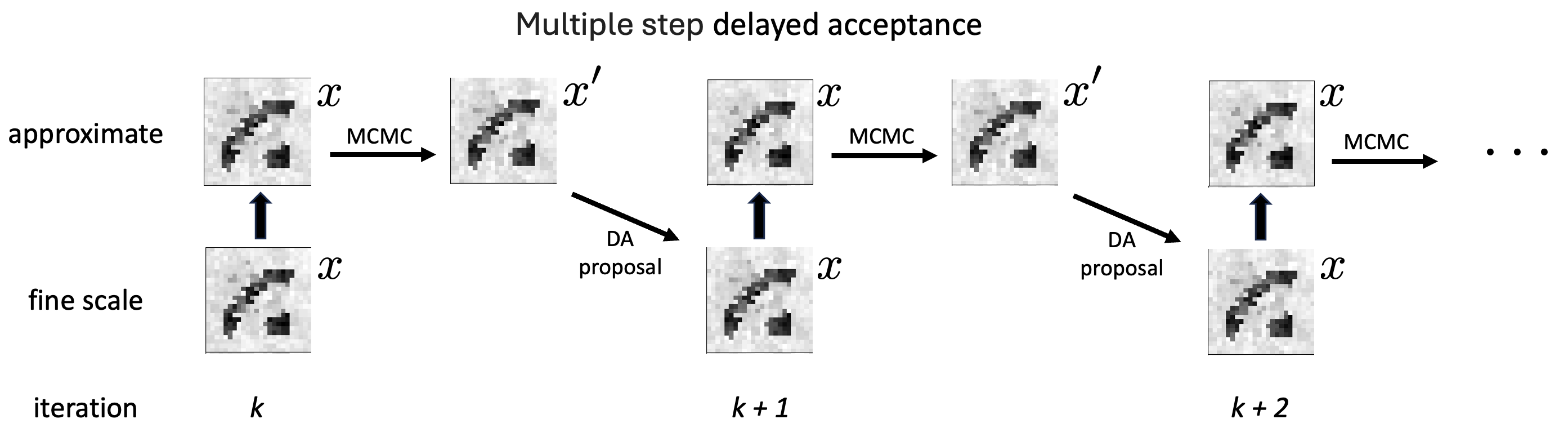
Multiple step delayed acceptance Algorithm 3 “filters” each proposal (step 4) before computing an acceptance outcome (step 6). Alternatively, multiple MCMC steps may be taken on the approximate formulation to produce a candidate that differs from the current state at more than just a single site .
This multiple step delayed acceptance (MSDA) is detailed in Algorithm 4. This algorithm produces updates that are in detailed balance with the fine scale posterior (Liu,, 2001; Lykkegaard et al.,, 2023). Figure 16.9 depicts this algorithm; now the horizontal arrows () denote single site MCMC steps using the approximate posterior as the target distribution. The collection of multiple steps needs to define a Markov kernel that is in detailed balance with the approximate posterior for the second acceptance probability (step 10 in Alg. 4) to be correct and give an algorithm that produces draws from . Randomly choosing the site to update (step 5, Alg. 4) achieves this, whereas the deterministic scan in Algorithm 1 does not.
This MSDA algorithm is very similar to one half of Metropolis coupling, by following a single flow of arrows in Figure 16.8 – the acceptance of the swap proposal in MC-MCMC is identical to acceptance of the eventual proposal produced by MSDA. However, there are major differences. MC-MCMC requires stationarity on the joint product distribution . MSDA aims for stationarity only on the fine scale posterior . The moves made according to the approximate posterior effectively produce a multivariate proposal to be considered at the fine scale. If is small, the proposal is “close” to the fine scale posterior; if very large, the proposal is closer to the approximate posterior. Hence, could serve as an MCMC tuning parameter, much like the proposal width used for the single site Metropolis steps. For the example in Section 4.3, we take .
Finally, we note that Christen and Fox, (2005) and Fox et al., (2020) give a more general formulation for the delayed acceptance sampler for which the approximate simulator can depend on the current state of the chain; the computed example in Christen and Fox, (2005) used a state-dependent linearization of the forward map. While a bit more demanding computationally, the more general algorithm can gain further efficiency by making use of local approximations and error models. Additionally, we remark that while we used a coarsened grid to construct the approximate simulator, any computationally cheaper approximation can be employed. Depending on the broader context of the problem, options include reduced-precision computing (Higham and Mary,, 2022), early stopping of iterative solvers (Wikle et al.,, 2001), early termination of time-dependent problems (Lykkegaard et al.,, 2023), dataset subsampling (Quiroz et al.,, 2019), reduced grid resolution (Lykkegaard et al.,, 2023), surrogate models (Laloy et al.,, 2013; Seelinger et al.,, 2024), and partially-computed likelihoods (Banterle et al.,, 2019).
4.3 Adaptive, multiple step delayed acceptance
So far, the coarse solver-based forward model has been ineffective in these MC-MCMC or MSDA implementations, in spite of its over 100-fold speed up in evaluating . This is because the coarse scale simulator differs too much from the fine scale simulator ; simply swapping out the fine with the coarse simulator in results in a posterior that is too far away from the target . Figure 16.10 shows the difference for the conductivity field shown in the left hand frame of Figure 16.7. The difference is largest at the injector electrodes.
Accounting for bias and error due to using an approximate model in place of the accurate, fine scale model has been a focus in Bayesian inverse problems (Kaipio and Somersalo,, 2007) and in computer model emulation (Kennedy and O’Hagan,, 2000). Here we follow Cui et al., (2011) and Fox et al., (2020) and use adaptive MCMC (Roberts and Rosenthal,, 2009, 2007) to adapt a “coarse” likelihood so that multiple step proposals are more readily accepted in DA. At step , is modified with an adaptive bias -vector and a covariance matrix
This gives an adaptive version of the coarse scale posterior . This adaptive, multiple step delayed acceptance algorithm is described in Algorithm 5.
Our implementation takes , , and initializes and . Figure 16.11 shows the MCMC histories for the same three conductivity pixels shown in previous figures. The computational effort is equivalent to that of Figure 16.4 – the equivalent of 40, forward model runs on the fine scale. After many iterations, the adaptive components and stabilize; the resulting values for are given by the dash (-) symbols in Figure 16.10.
We employed the free and open-source Python software library tinyDA (Lykkegaard,, 2023) for the numerical experiments involving Delayed Acceptance MCMC outlined here. In addition to standard Metropolis-Hastings, DA and MSDA MCMC, tinyDA provides routines for Multilevel Delayed Acceptance (MLDA), a multilevel extension to MSDA, which enables MCMC sampling using a multilevel hierarchy of increasingly coarser models (Lykkegaard et al.,, 2023). When carefully implemented, such a multilevel model hierarchy can provide even higher gains to the MCMC sampling efficiency than the two-level sampler employed in this work.
5 Discussion
For the EIT example, single-site Metropolis requires about 20 million simulator evaluations to effectively sample this posterior distribution. Multivariate updating schemes such as random walk Metropolis or DE-MCMC – as we implemented them here, or in the previous version of this chapter – don’t offer any real relief. Tempering and Metropolis-coupling schemes can help if the approximate forward model is very close to the fine scale forward model. Here the multigrid-based approximation is quite accurate, but is only three times faster. Hence the speed-up with such a model will be of a similar magnitude. The AMSDA approach using the much faster (over ) coarse forward model seems to be an exception. The combination of the adaptive error term and the multiple steps before testing the candidate with the expensive, fine-scale forward model results in an MCMC scheme that is over an order of magnitude more efficient. The success of this approach with other challenging inverse problems (Fox et al.,, 2020; Lykkegaard et al.,, 2023) suggests this isn’t just due to the special features of this particular EIT example. We also note that for ease of presentation, we have described rather basic implementations of delayed acceptance schemes. We point the reader to Fox et al., (2020), Banterle et al., (2019) and Lykkegaard et al., (2023) for richer implementations.
One challenging feature of this application is the multimodal nature of the posterior which is largely induced by our choice of prior. By specifying a more regularizing prior, such as the GMRF 2.3) or the process convolution (6.1), the resulting posterior will more likely be unimodal, so that standard MCMC schemes will be more efficient. Of course, the sacrifice is that one is now less able to recover small-scale structure that may be present in the inverse problem.
We considered two different fast, approximate simulators in this chapter. There is a rather vast literature developing fast approximations to computationally intensive models. This includes reduced order models (Benner et al.,, 2017), cross approximations (Dolgov and Scheichl,, 2019), and response surface/regression approaches such as polynomial chaos (Xiu and Karniadakis,, 2002), Gaussian processes (Kennedy and O’Hagan,, 2001), or additive regression trees (Pratola and Higdon,, 2016). The response surface approaches are most useful when the effective dimension of the parameter vector is fairly small () and the output response to parameter changes is smooth and predictable. The response surface is typically estimated from a collection of model runs carried out at different input parameter settings. By contrast, a well designed reduced order model can enable MCMC to handle some rather complicated high-dimensional, non-linear problems – see Keating et al., (2010), for example. A comparison of reduced model and response surface approaches can be found in Frangos et al., (2010).
Finally we note that the traditional way to speed up the computation required to solve an inverse problem is to speed up the simulator . A substantial amount of progress has been made to create simulators that run on highly distributed computing machines. While MCMC does not lend itself to easy parallelization, we are seeing advances in the use of parallelized MCMC for inverse problems (Craiu et al.,, 2009; Vrugt,, 2016; Nishihara et al.,, 2014; Conrad et al.,, 2018; Brockwell,, 2006). The integration of modern computing architecture with MCMC methods will certainly extend the reach of MCMC based solutions to inverse problems.
Acknowledgments
DH was supported, in part, by the U.S. Department of Energy, Office of Science, Office of Advanced Scientific Computing Research and Office of High Energy Physics, Scientific Discovery through Advanced Computing (SciDAC) program. CF is grateful to digiLab for support and a pleasant working environment.
References
- Andersen et al., (2003) Andersen, K., Brooks, S., and Hansen, M. (2003). Bayesian inversion of geoelectrical resistivity data. Journal of the Royal Statistical Society: Series B, 65(3):619–642.
- Banterle et al., (2019) Banterle, M., Grazian, C., Lee, A., and Robert, C. P. (2019). Accelerating Metropolis-Hastings algorithms by delayed acceptance. Foundations of Data Science, 1(2):103–128.
- Benner et al., (2017) Benner, P., Cohen, A., Ohlberger, M., and Willcox, K. (2017). Model reduction and approximation: theory and algorithms. Computational Science and Engineering. SIAM.
- Brockwell, (2006) Brockwell, A. E. (2006). Parallel Markov chain Monte Carlo simulation by pre-fetching. Journal of Computational and Graphical Statistics, 15(1):246–261.
- Christen and Fox, (2005) Christen, J. and Fox, C. (2005). Markov chain Monte Carlo using an approximation. Journal of Computational & Graphical Statistics, 14(4):795–810.
- Cleveland, (1979) Cleveland, W. S. (1979). Robust locally weighted regression and smoothing scatterplots. Journal of the American Statistical Association, 74:829–836.
- Conrad et al., (2018) Conrad, P. R., Davis, A. D., Marzouk, Y. M., Pillai, N. S., and Smith, A. (2018). Parallel local approximation MCMC for expensive models. SIAM/ASA Journal on Uncertainty Quantification, 6(1):339–373.
- Craiu et al., (2009) Craiu, R. V., Rosenthal, J., and Yang, C. (2009). Learn from thy neighbor: Parallel-chain and regional adaptive MCMC. Journal of the American Statistical Association, 104(488):1454–1466.
- Cui et al., (2011) Cui, T., Fox, C., and O’Sullivan, M. J. (2011). Bayesian calibration of a large-scale geothermal reservoir model by a new adaptive delayed acceptance Metropolis Hastings algorithm. Water Resources Research, 47(10).
- Dendy, (1982) Dendy, J. E. (1982). Black box multigrid. J. Comput. Phys., 48:366–386.
- Dolgov and Scheichl, (2019) Dolgov, S. and Scheichl, R. (2019). A hybrid alternating least squares–TT cross algorithm for parametric PDEs. SIAM/ASA Journal on Uncertainty Quantification, 7(1):260–291.
- Edwards and Sokal, (1988) Edwards, R. G. and Sokal, A. D. (1988). Generalization of the Fortuin-Kasteleyn-Swendsen-Wang representation and Monte Carlo algorithm. Physical Review Letters, 38:2009–2012.
- Fox et al., (2020) Fox, C., Cui, T., and Neumayer, M. (2020). Randomized reduced forward models for efficient Metropolis–Hastings MCMC, with application to subsurface fluid flow and capacitance tomography. GEM-International Journal on Geomathematics, 11:1–38.
- Fox and Nicholls, (1997) Fox, C. and Nicholls, G. (1997). Sampling conductivity images via MCMC. The art and science of Bayesian image analysis. Proceedings of the Leeds annual statistics research workshop, pages 91–100.
- Frangos et al., (2010) Frangos, M., Marzouk, Y., Willcox, K., and van Bloemen Waanders, B. (2010). Surrogate and reduced-order modeling: a comparison of approaches for large-scale statistical inverse problems. Large-Scale Inverse Problems and Quantification of Uncertainty, pages 123–149.
- Frigessi et al., (1993) Frigessi, A., Stefano, P. D., Hwang, C.-R., and Sheu, S.-J. (1993). Convergence rates of the Gibbs sampler, the Metropolis algorithm and other single-site updating dynamics. Journal of the Royal Statistical Society. Series B (Methodological), 55(1):205–219.
- Gelman et al., (1996) Gelman, A., Roberts, G., and Gilks, W. (1996). Efficient Metropolis jumping rules. Bayesian Statistics 5: Proceedings of the Fifth Valencia International Meeting, June 5-9, 1994.
- Geman and McClure, (1987) Geman, S. and McClure, D. (1987). Statistical methods for tomographic image reconstruction. Bulliten of the International Statistical Institute, 52:no.4 5–21.
- Geyer, (1991) Geyer, C. J. (1991). Monte Carlo maximum likelihood for dependent data. In Keramidas, E., editor, Computer Science and Statistics: Proceedings of the 23rd Symposium Interface, pages 156–163.
- Haario et al., (2006) Haario, H., Laine, M., Mira, A., and Saksman, E. (2006). DRAM: efficient adaptive MCMC. Statistics and computing, 16:339–354.
- Higdon, (2002) Higdon, D. (2002). Space and space-time modeling using process convolutions. In Anderson, C., Barnett, V., Chatwin, P. C., and El-Shaarawi, A. H., editors, Quantitative Methods for Current Environmental Issues, pages 37–56, London. Springer Verlag.
- Higdon et al., (2002) Higdon, D., Lee, H., and Bi, Z. (2002). A Bayesian approach to characterizing uncertainty in inverse problems using coarse and fine scale information. IEEE Transactions in Signal Processing, 50:389–399.
- Higdon et al., (2011) Higdon, D., Reese, C. S., Moulton, J. D., Vrugt, J. A., and Fox, C. (2011). Posterior exploration for computationally intensive forward models. Handbook of Markov Chain Monte Carlo, pages 401–418.
- Higdon, (1998) Higdon, D. M. (1998). Auxiliary variable methods for Markov chain Monte Carlo with applications. Journal of the American Statistical Association, 93:585–595.
- Higdon et al., (2003) Higdon, D. M., Lee, H., and Holloman, C. (2003). Markov chain Monte Carlo-based approaches for inference in computationally intensive inverse problems. In Bernardo, J. M., Bayarri, M. J., Berger, J. O., Dawid, A. P., Heckerman, D., Smith, A. F. M., and West, M., editors, Bayesian Statistics 7. Proceedings of the Seventh Valencia International Meeting, pages 181–197. Oxford University Press.
- Higham and Mary, (2022) Higham, N. J. and Mary, T. (2022). Mixed precision algorithms in numerical linear algebra. Acta Numerica. Publisher: Cambridge University Press (CUP).
- Jimenez et al., (2004) Jimenez, R., Verde, L., Peiris, H., and Kosowsky, A. (2004). Fast cosmological parameter estimation from microwave background temperature and polarization power spectra. Physical Review D, 70(2):23005.
- Kaipio et al., (2000) Kaipio, J., Kolehmainen, V., Somersalo, E., and Vauhkonen, M. (2000). Statistical inversion and Monte Carlo sampling methods in electrical impedance tomography. INVERSE PROBL, 16(5):1487–1522.
- Kaipio and Somersalo, (2007) Kaipio, J. and Somersalo, E. (2007). Statistical inverse problems: discretization, model reduction and inverse crimes. Journal of computational and applied mathematics, 198(2):493–504.
- Kaipio and Somersalo, (2004) Kaipio, J. P. and Somersalo, E. (2004). Statistical and Computational Inverse Problems. Springer, New York.
- Keating et al., (2010) Keating, E. H., Doherty, J., Vrugt, J. A., and Kang, Q. (2010). Optimization and uncertainty assessment of strongly nonlinear groundwater models with high parameter dimensionality. Water Resources Research, 46(10).
- Kennedy and O’Hagan, (2000) Kennedy, M. and O’Hagan, A. (2000). Predicting the output from a complex computer code when fast approximations are available. Biometrika, 87:1–13.
- Kennedy and O’Hagan, (2001) Kennedy, M. and O’Hagan, A. (2001). Bayesian calibration of computer models (with discussion). Journal of the Royal Statistical Society (Series B), 68:425–464.
- Laloy et al., (2013) Laloy, E., Rogiers, B., Vrugt, J. A., Mallants, D., and Jacques, D. (2013). Efficient posterior exploration of a high-dimensional groundwater model from two-stage Markov chain Monte Carlo simulation and polynomial chaos expansion. Water Resources Research, 49(5):2664–2682.
- Liu, (2001) Liu, J. (2001). Monte Carlo Strategies in Scientific Computing. Springer.
- Liu and Sabatti, (1999) Liu, J. and Sabatti, C. (1999). Simulated sintering: Markov chain Monte Carlo with spaces of varying dimensions. Bayesian Statistics 6: Proceedings of the Sixth Valencia International Meeting, June 6-10, 1998.
- Lykkegaard, (2023) Lykkegaard, M. B. (2023). tinyDA. https://github.com/mikkelbue/tinyDA.
- Lykkegaard et al., (2023) Lykkegaard, M. B., Dodwell, T. J., Fox, C., Mingas, G., and Scheichl, R. (2023). Multilevel delayed acceptance MCMC. SIAM/ASA Journal on Uncertainty Quantification, 11(1):1–30.
- Marinari and Parisi, (1992) Marinari, E. and Parisi, G. (1992). Simulated tempering: a new Monte Carlo scheme. Europhysics Letters, 19:451–458.
- Metropolis et al., (1953) Metropolis, N., Rosenbluth, A., Rosenbluth, M., Teller, A., and Teller, E. (1953). Equations of state calculations by fast computing machines. Journal of Chemical Physics, 21:1087–1091.
- Moulton et al., (2008) Moulton, J. D., Fox, C., and Svyatskiy, D. (2008). Multilevel approximations in sample-based inversion from the Dirichlet-to-Neumann map. J. Phys.: Conf. Ser., 124:012035 (10pp).
- Nickl, (2023) Nickl, R. (2023). Bayesian Non-linear Statistical Inverse Problems. EMS Press.
- Nishihara et al., (2014) Nishihara, R., Murray, I., and Adams, R. P. (2014). Parallel MCMC with generalized elliptical slice sampling. The Journal of Machine Learning Research, 15(1):2087–2112.
- Nissinen et al., (2008) Nissinen, A., Heikkinen, L. M., and Kaipio, J. P. (2008). The Bayesian approximation error approach for electrical impedance tomography; experimental results. Meas. Sci. Technol., 19(1):015501 (9pp).
- Paciorek and Schervish, (2004) Paciorek, C. J. and Schervish, M. J. (2004). Nonstationary covariance functions for Gaussian process regression. In Thrun, S., Saul, L., and Schölkopf, B., editors, Advances in Neural Information Processing Systems 16. MIT Press, Cambridge, MA.
- Pratola and Higdon, (2016) Pratola, M. T. and Higdon, D. M. (2016). Bayesian additive regression tree calibration of complex high-dimensional computer models. Technometrics, 58(2):166–179.
- Quiroz et al., (2019) Quiroz, M., Kohn, R., Villani, M., and Tran, M.-N. (2019). Speeding up MCMC by efficient data subsampling. Journal of the American Statistical Association, 114(526):831–843.
- Roberts and Rosenthal, (2007) Roberts, G. O. and Rosenthal, J. S. (2007). Coupling and ergodicity of adaptive Markov chain Monte Carlo algorithms. Journal of applied probability, 44(2):458–475.
- Roberts and Rosenthal, (2009) Roberts, G. O. and Rosenthal, J. S. (2009). Examples of adaptive MCMC. Journal of computational and graphical statistics, 18(2):349–367.
- Rue, (2001) Rue, H. (2001). Fast sampling of Gaussian Markov random fields. Journal of the Royal Statistical Society: Series B, 63(2):325–338.
- Seelinger et al., (2024) Seelinger, L., Reinarz, A., Lykkegaard, M. B., Alghamdi, A. M. A., Aristoff, D., Bangerth, W., Bénézech, J., Diez, M., Frey, K., Jakeman, J. D., Jørgensen, J. S., Kim, K.-T., Martinelli, M., Parno, M., Pellegrini, R., Petra, N., Riis, N. A. B., Rosenfeld, K., Serani, A., Tamellini, L., Villa, U., Dodwell, T. J., and Scheichl, R. (2024). Democratizing Uncertainty Quantification. arXiv:2402.13768 [cs, stat].
- Stenerud et al., (2008) Stenerud, V. R., Kippe, V., Lie, K. A., and Datta-Gupta, A. (2008). Adaptive multiscale streamline simulation and inversion for high-resolution geomodels. SPE Journal, 13(01):99–111.
- Taghizadeh et al., (2020) Taghizadeh, L., Karimi, A., Stadlbauer, B., Weninger, W. J., Kaniusas, E., and Heitzinger, C. (2020). Bayesian inversion for electrical-impedance tomography in medical imaging using the nonlinear Poisson–Boltzmann equation. Computer Methods in Applied Mechanics and Engineering, 365:112959.
- ter Braak, (2006) ter Braak, C. F. J. (2006). A Markov Chain Monte Carlo version of the genetic algorithm Differential Evolution: easy Bayesian computing for real parameter spaces. Statistics and Computing, 16(3):239–249.
- Tierney, (1994) Tierney, L. (1994). Markov chains for exploring posterior distributions (with discussion). Annals of Statistics, 21:1701–1762.
- Vrugt, (2016) Vrugt, J. A. (2016). Markov chain Monte Carlo simulation using the DREAM software package: Theory, concepts, and MATLAB implementation. Environmental Modelling & Software, 75:273–316.
- Weir, (1997) Weir, I. (1997). Fully Bayesian reconstructions from single photon emission computed tomography. Journal of the American Statistical Association, 92:49–60.
- Wikle et al., (2001) Wikle, C. K., Milliff, R. F., Nychka, D., and Berliner, L. M. (2001). Spatiotemporal Hierarchical Bayesian Modeling: Tropical Ocean Surface Winds. Journal of the American Statistical Association, 96(454):382–397.
- Xiu and Karniadakis, (2002) Xiu, D. and Karniadakis, G. E. (2002). The Wiener–Askey polynomial chaos for stochastic differential equations. SIAM journal on Scientific Computing, 24(2):619–644.
6 Formulation based on a process convolution prior
An alternative to treating each pixel in the image as a parameter to be estimated is to use a lower dimensional representation for the prior. Here we describe a process convolution (Higdon,, 2002) prior for the underlying image .
We define to be a mean zero Gaussian process. But rather than specify through its covariance function, it is determined by a latent process and a smoothing kernel . The latent process is located at the spatial sites , also in (shown in Figure 12). The ’s are then modeled as independent draws from a distribution. The resulting continuous Gaussian process model for is then
| (6.1) |
where is a kernel centered at . For the EIT application, we define the smoothing kernel to be a radially symmetric bivariate Gaussian density, with standard deviation . Figure 12 shows a prior draw from this model over the pixel sites in .
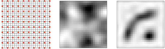
Under this formulation, the image is controlled by parameters in . Thus a single-site Metropolis scan of takes less than 20% of the computational effort required to update each pixel in . In addition, this prior enforces very smooth realizations for . This makes the posterior distribution better behaved, but may make posterior realizations of unreasonably smooth. The resulting posterior mean for is shown in Figure 12. For a more detailed look at process convolution models, see (Higdon,, 2002); Paciorek and Schervish, (2004) give non-stationary extensions of these spatial models.