Adaptive Bidirectional Displacement for Semi-Supervised Medical Image Segmentation
Abstract
Consistency learning is a central strategy to tackle unlabeled data in semi-supervised medical image segmentation (SSMIS), which enforces the model to produce consistent predictions under the perturbation. However, most current approaches solely focus on utilizing a specific single perturbation, which can only cope with limited cases, while employing multiple perturbations simultaneously is hard to guarantee the quality of consistency learning. In this paper, we propose an Adaptive Bidirectional Displacement (ABD) approach to solve the above challenge. Specifically, we first design a bidirectional patch displacement based on reliable prediction confidence for unlabeled data to generate new samples, which can effectively suppress uncontrollable regions and still retain the influence of input perturbations. Meanwhile, to enforce the model to learn the potentially uncontrollable content, a bidirectional displacement operation with inverse confidence is proposed for the labeled images, which generates samples with more unreliable information to facilitate model learning. Extensive experiments show that ABD achieves new state-of-the-art performances for SSMIS, significantly improving different baselines. Source code is available at https://github.com/chy-upc/ABD.
1 Introduction
Medical image segmentation derives from computer tomography (CT) or magnetic resonance imaging (MRI), which is crucial for various clinical applications [34, 45]. Obtaining a large medical dataset with precise annotation to train segmentation models is challenging, as reliable annotations can only be provided by experts, which constrains the development of medical image segmentation algorithms and poses substantial challenges for further research and implementation [31, 43]. To mitigate the burden of manual annotation and address these challenges, semi-supervised medical image segmentation (SSMIS) [28, 35, 2, 42] is emerging as a practical approach to encourage segmentation models to learn from readily available unlabelled data in conjunction with limited labeled examples.

Most recent approaches in SSMIS employ consistency learning [11, 44, 9, 15] to make the decision boundary of the learned model located within the low-density boundary [12]. By ensuring consistent features or predictions under diverse perturbations, this strategy becomes one of the most effective solutions for learning from unlabelled data. According to the perturbation differences, consistency learning approaches can be divided into three categories: 1) Input perturbations, which mainly produce different inputs to the same model [5, 29, 41], e.g., weak and strong data augmentation for the given image. 2) Feature perturbations [25, 47, 17], which mainly include feature noise, feature dropout, and context masking. 3) Network perturbations [13, 8], which focus on using different network architectures for the same input. To ensure the stability of consistency learning, most previous approaches [32, 51, 16, 38] solely utilize one of the above perturbations, restricting the performance of the consistency learning and leading to imprecise decision boundary since the specific single perturbation can only handle limited cases, as shown in Fig. 1(a).
Utilizing mixed or multiple perturbations presents a direct solution to solve the above problem. However, once added multiple perturbations, the consistency learning process is easily out-of-control, leading to restricted learning quality. For example, Cross Pseudo Supervision (CPS) [8] is a widely-used technique in consistency learning that primarily applies network perturbation to produce two discriminate predictions for further consistency learning. If we directly add input perturbation by using weak and strong augmentation to the input training data, consistency learning will be ineffective. As shown in Fig. 1(b), when the original input is replaced with weak and strong augmentation inputs, the CPS model incorrectly classifies the background as the foreground with consistency learning mechanism, indicating decreased performance when mixed perturbations are introduced.
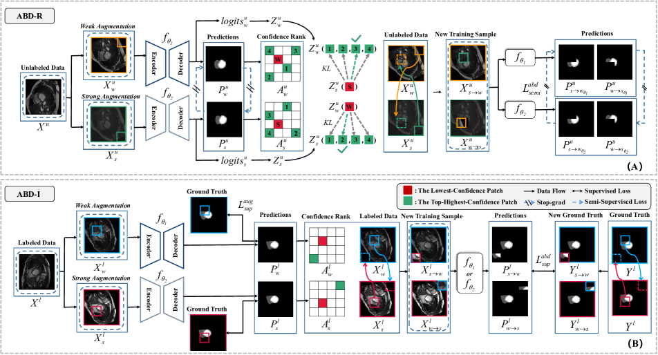
To tackle the aforementioned challenges, we propose Adaptive Bidirectional Displacement (ABD) for SSMIS, as shown in Fig. 1(c). Specifically, for each unlabelled image, the input perturbation is firstly applied to produce a pair of input images, e.g., weak augmentation image and strong augmentation image. Then we generate two confidence matrices (confidence rank maps) based on the predictions from the above two perturbed images. The confidence matrix assesses the certainty of predicted pixels belonging to various categories, thereby reflecting the model’s reliability to different perturbations. Then, for any augmented image, its region with the lowest confidence rank is displaced with the region from the other augmented image that has the most similar output distribution with highly confident scores. We refer to this as an adaptive bidirectional displacement with reliable confidence (ABD-R). In this way, the newly generated image can remove the uncontrolled region and obtain complementary and approximate semantic information from another augmented image, which ensures consistent predictions of the model across different perturbations. Meanwhile, to enforce the model to learn those potentially uncontrollable regions, we incorporate inverse confidence for labeled data as an additional adaptive bidirectional displacement (ABD-I). For any labeled augmented image, the image regions with the highest confidence scores are displaced with the regions from another augmented image having the lowest confidence scores. This operation will strengthen the model to tackle uncontrollable regions. Combining these two strategies, our approach performs a novel input perturbation method, which can be directly applied to existing consistency learning approaches. Extensive experiments show that ABD achieves new state-of-the-art (SOTA) performances for SSMIS, significantly improving different baseline performances.
We summarize our main contributions as follows:
-
•
We observed that the combination of different perturbations leads to instability in consistency learning. To address this issue, we propose Adaptive Bidirectional Displacement to enable the generation of semantically complementary data by replacing model inadaptable regions with credible regions, which assists the model in effectively correcting erroneous predictions and enhances the quality of consistency learning.
-
•
To take full advantage of labeled data, we propose an enhanced Adaptive Bidirectional Displacement that incorporates inverse confidence for labeled data to enforce the model to tackle those potentially uncontrollable regions.
-
•
The proposed method can be easily plug-and-play, which can be embedded into different approaches and enhance their performance. Extensive experiments are conducted to validate the feasibility of the method, resulting in significant improvements compared to previous SOTA approaches on different datasets.
2 Related Work
2.1 Consistency Learning in Semi-Supervised Medical Image Segmentation
Consistency learning has been widely used in recent approaches for SSMIS. It aims to improve the performance of models by promoting consistent predictions for unlabeled data under different perturbations. According to the perturbation differences, consistency learning has three categories: input perturbation, feature perturbation, and network perturbation. Input perturbation is achieved through producing different inputs. For instance, Huang et al. [11] introduced cutout content loss and slice misalignment as perturbations in the input. In contrast, ST++ [39] involved strong augmentation on unlabeled images and directly utilizes the augmented samples for re-training. PseudoSeg [51] was similar to FixMatch [30] in leveraging pseudo-labels generated from weakly augmented images to supervise the predictions of strongly augmented images. BCP [2] encouraged the mixing of labeled and unlabeled images on the input level, enabling unlabeled data to learn comprehensive and general semantic information from labeled data in both directions. Meanwhile, feature perturbation and network perturbation are achieved by producing different features or outputs for the same input. Specifically, for feature perturbation, Mismatch [38] introduced morphological feature perturbation, which is based on classic morphological operations. For network perturbation, CPS [8] encouraged consistent predictions from different initialized networks with an input image. Mean Teacher [32] utilized the exponential moving average (EMA) technique to transfer semantic knowledge from the student network to the teacher network. However, existing methods only guarantee the consistency of predictions under a single perturbation, which greatly limits the scalability of consistency learning.
2.2 Consistency Learning in Other Tasks
Consistency learning [46, 18] is a major technique to tackle unlabeled data in semi-supervised learning. Several methods are proposed with consistency learning in various domains, including image segmentation [40, 26], domain generalization [50, 49], image classification [48, 33], pre-train language model [10], etc. For image segmentation, Revisiting UniMatch [40] proposed a unified approach using dual-stream perturbations for semi-supervised semantic segmentation by combining input and feature perturbations. Additionally, ViewCo [26] introduced text-to-view consistency modeling, incorporating additional text to learn comprehensive segmentation masks. In domain generalization, Zhou et al. [50] exploited the latent uncertainty information of the unlabeled samples to design an uncertainty-guided consistency loss. StyleMatch [49] enforced prediction consistency between images from one domain and their style-transferred counterparts. In image classification, SimMatch [48] applied consistency regularization on both the semantic level and instance level to generate high-quality and reliable targets. ICT [33] introduced the interpolation consistency training which encourages the prediction at an interpolation of unlabeled points to be consistent with the interpolation of the predictions at those points. In addition, in the pre-train language model, GALAXY [10] applied consistency regularization on all data to minimize the bi-directional KL divergence between model predictions.
3 Method
3.1 Problem Setting
In the semi-supervised segmentation, we utilize a labeled dataset along with an unlabeled dataset . Here, represents a labeled image and represents its corresponding label. Similarly, denotes an unlabeled image. For convenience, will be omitted in the following part. It is worth emphasizing that the number of labeled images is significantly larger than the number of unlabeled images, i.e., .
3.2 Overview
The overall framework of our approach is shown in Fig. 2, which can be divided into the following steps:
-
1.
For the input labeled image, we first apply input perturbation to generate two different samples, e.g., a weak augmentation image and a strong augmentation image, both of which are input to the model with network perturbation: the weak augmentation image is input to one network and the strong augmentation image is input to the other network to generate two corresponding predictions, using the provided label as supervision.
-
2.
For an unlabeled image, two predictions are obtained following the above pipeline. Then using our proposed ABD-R, the corresponding confidence matrices are used to perform bidirectional displacement between two augmented unlabeled images to generate new input samples.
-
3.
Meanwhile, to enforce learning from the potentially uncontrollable regions, the ABD-I strategy based on inverse confidence is applied to labeled data to generate two new samples with the corresponding labels.
-
4.
Finally, all generated new samples are input to the model to produce the corresponding predictions. The predictions of unlabeled data are used for cross-supervision, and the predictions of labeled data are supervised by the newly generated labels.
3.3 Adaptive Bidirectional Displacement with Reliable Confidence
Under various perturbations, the segmentation model produces unreliable predictions for unlabeled data. Imposing alignment using these predictions can render consistent learning ineffective. A direct solution is to remove the regions related to unreliable prediction. In practice, we first generate the confidence matrix based on the model’s predictions. The confidence matrix measures the confidence of each predicted pixel belonging to different categories, it reflects the model’s reliability to different perturbations. Utilizing the confidence matrix, our ABD-R can generate a new training sample that exhibits more reliable regions.
Suppose is an unlabeled medical image with weak augmentation. is the same unlabeled medical image but with strong augmentation. After passing the model, we generate their corresponding outputs:
| (1) |
where and are two networks, which usually have different architecture or initialization to build the network perturbation. and are the logits outputs that correspond to and , respectively. Applying softmax to these logits yields the corresponding prediction probability scores:
|
|
(2) |
where is the prediction of and is the prediction of . After upsampling them to the same height and width with input, we can generate and . is the number of classes.
Then we divide into patches, each with a size of , denoting as , where and . For any patch ( is the index of the patch), the corresponding logits outputs are represented as and predictions are represented as .
Then, for each patch of , its logits scores is:
| (3) |
where represents the average logits score of the -th patch for the class and , is the logit score of the class for the -th pixel in the -th patch. We regard as the output distribution for the -th patch of .
Meanwhile, the corresponding confidence score for the -th patch is computed as follows:
| (4) |
where is the index of the corresponding patch, is the probability of the class for the -th pixel in the patch. is a maximum operator to select the highest confidence score for each pixel. is the average confidence score for the -th patch, which measures the reliability of the corresponding patch.
Then the index of the patch with the lowest confidence for is computed as:
| (5) |
Simultaneously, using the confidence map , the top highest confidence patches in are selected, and the corresponding index set is represented as:
| (6) |
where is an index set that includes the indices of the selected top highest confidence patches. is the selected indices, for example, is the index of the patch that has the highest (top 1) confidence score.
Similarly, following the above operations, we divide into patches, the corresponding logits and confidence score are represented as and , respectively. After processing from Eq. (5) to Eq. (6), the indices of the top-highest and the lowest confidence for are generated, representing as and , respectively. And
To achieve controlled effects of the mixed perturbations and enhance semantic coherence of the displacement operation, we select the most similar patch from the obtained index sets ( and ) by calculating the difference of the output distribution between the selected top- highest confidence patches in one image and the lowest confidence patch in the other image:
|
|
(7) |
where is to compute the KL divergence [14], e.g., , which reflects the difference in the output distribution. and represent the indices of final selected patches.
Finally, the bidirectional displacement operation is performed for and . The patch of one augmented image with the lowest confidence score is displaced with the final selected patch from the other augmented image:
| (8) |
| (9) |
After removing the patching operation and reshaping them to the image, two new samples and are generated, which are then input to two networks and for cross-supervision, as shown in Eq. (18).
This approach allows the two networks to adapt to each other’s input perturbations, resulting in higher quality and more reliable pseudo-labels. As a cross-supervised process for the unlabeled data, it also reduces the likelihood of one model making erroneous predictions, thereby preventing the degradation of the other model’s training process.
3.4 Adaptive Bidirectional Displacement with Inverse Confidence
In the above ABD-R module, unlabeled images are manipulated to create new samples by replacing the potentially uncontrollable patches with new patches, it does not directly learn from the original regions. To enforce the model to learn from these potentially uncontrollable regions, we propose Adaptive Bidirectional Displacement with Inverse Confidence (ABD-I) for the labeled images to strengthen the learning for uncontrollable regions.
Specifically, for a labeled image , we perform a strong augmentation to obtain a sample and a weak augmentation to obtain a sample . Let as an example, we execute Eq. (1) to Eq. (6) on to get its region index, i.e., and . Similarly, we repeat the above operation for the strong augmented image to get and . Note that and are the indices of the patches that have the highest (top 1) confidence score, we directly use them rather than selecting from candidates since these regions are the most potentially controllable region and we do not need to consider the semantic coherence with the given annotations. and share the same definition with Eq. (5).
Then ABD-I is used, the region of one image with the highest confidence scores is displaced with the region from the other image having the lowest confidence scores:
| (10) |
| (11) |
Using Eq. (10) and Eq. (11), the new samples and are generated. To effectively supervise the displaced samples, the same displacement is applied to the original label. Suppose is the label of images and , we also divide into patches, denoting as . The corresponding displacement operation is expressed as:
| (12) |
| (13) |
Finally and are used to supervise the generated samples and , as shown in Eq. (16).
3.5 Loss Functions
The overall loss function consists of two parts, the supervised loss for labeled data and the unsupervised loss for unlabeled data, defined as:
| (14) | ||||
where is a weight that balances different losses, which gradually increase with iterations increases based on the Gaussian warming up: , is the current iteration and is the total iteration.
The consists of and . is used for the original augmented labeled images, is used for the newly generated labeled samples.
The loss is computed as:
|
|
(15) |
where , are the cross-entropy loss and dice loss [24], respectively. is the label.
The loss is computed as:
| (16) | |||
The unsupervised loss consists of and . is used for the original augmented unlabeled images, is for the newly generated unlabeled images.
Method Scans used Metrics Labeled Unlabeled DSC Jaccard 95HD ASD U-Net (MICCAI’2015) [27] 3(5%) 0 47.83 37.01 31.16 12.62 7(10%) 0 79.41 68.11 9.35 2.70 70(All) 0 91.44 84.59 4.30 0.99 DTC (AAAI’2021) [21] 3(5%) 67(95%) 56.90 45.67 23.36 7.39 URPC (MICCAI’2021) [22] 55.87 44.64 13.60 3.74 MC-Net (MICCAI’2021) [36] 62.85 52.29 7.62 2.33 SS-Net (MICCAI’2022) [37] 65.83 55.38 6.67 2.28 SCP-Net (MICCAI’2023) [44] 87.27 - - 2.65 Cross Teaching (Reported) (MIDL’2022) [23] 65.60 - 16.2 - BCP (CVPR’2023) [2] 87.59 78.67 1.90 0.67 Ours-ABD (Cross Teaching) 86.35 76.73 4.12 1.22 Ours-ABD (BCP) 88.96 80.70 1.57 0.52 DTC (AAAI’2021) [21] 7(10%) 63(90%) 84.29 73.92 12.81 4.01 URPC (MICCAI’2021) [22] 83.10 72.41 4.84 1.53 MC-Net (MICCAI’2021) [36] 86.44 77.04 5.50 1.84 SS-Net (MICCAI’2022) [37] 86.78 77.67 6.07 1.40 SCP-Net (MICCAI’2023) [44] 89.69 - - 0.73 PLGCL (CVPR’2023) [3] 89.1 - 4.98 1.80 Cross Teaching (Reported) (MIDL’2022) [23] 86.40 - 8.60 - Cross Teaching (Reproduced) 86.45 77.02 6.30 1.86 BCP (CVPR’2023) [2] 88.84 80.62 3.98 1.17 Ours-ABD (Cross Teaching) 88.52 79.97 5.06 1.43 Ours-ABD (BCP) 89.81 81.95 1.46 0.49
The loss function is defined as:
| (18) | |||
where and , which are the predictions from and , respectively. Similarly, and are obtained using the same operation.
4 Experiments
4.1 Dataset and Evaluation Metrics
ACDC dataset: The ACDC dataset [4] comprises 200 annotated short-axis cardiac cine-MR images from a cohort of 100 patients with four classes. 2D segmentation is more common than direct 3D segmentation [1]. The data split remains 70 patients’ scans for training, 10 for validation, and 20 for testing. Following previous approaches, four evaluation metrics are chosen: Dice Similarity Coefficient (DSC), Jaccard, 95% Hausdorff Distance (95HD) and Average Surface Distance (ASD).
PROMISE12 dataset: The PROMISE12 dataset [19] was made available for the MICCAI 2012 prostate segmentation challenge. MRI of 50 patients with various diseases was acquired at different locations. All 3D scans are converted into 2D slices. Following previous approaches, DSC and ASD are used as evaluation metrics.
4.2 Implementation Details
Cross Teaching [23] is a cross-supervision framework, which utilizes two networks to perform the network perturbation: and , representing UNet [27] and Swin-UNet [6], respectively. We add the input perturbation using weak and strong data augmentation to provide two kinds of inputs. For weak data augmentation, random rotation and flipping are used. For strong data augmentations, colorjitter, blur [7] and Cutout [39] are used. During training, all inputs are cropped to and divided into patches. The networks are trained with a batch size of 16, including 8 labeled slices and 8 unlabeled slices.
BCP [2] is a mean-teacher framework, which applies weak and strong augmentation to perform input perturbation. We add the network perturbation by providing two student networks with different initializations. Our ABD is used on these two student networks following the above design. During training, all inputs are cropped to and divided into patches.
4.3 Comparison with Sate-of-the-Art Methods
ACDA dataset: Table 1 shows the average performance on the ACDC dataset using 5% and 10% labeled ratios. For the 5% label ratio, our ABD achieves state-of-the-art performance compared to recent methods, surpassing the baseline Cross Teaching by a large margin. BCP is one of the newly released methods, it achieved high performance on the ACDC dataset. By incorporating our method into BCP, i.e., Ours-ABD (BCP), it has a noticeable improvement, which highlights the flexibility and scalability of our approach. Specifically, we observe a 20.75% DSC improvement compared to Cross Teaching and a 1.37% DSC improvement compared to BCP. Considering the 10% labeled ratio, our ABD outperforms SCP-Net [44] in all evaluation metrics and achieves a new state-of-the-art performance. It demonstrates that ABD mitigates the uncontrolled effects caused by the mixture of multiple perturbations and validates the mixed perturbations could expand the upper bound of consistency learning.
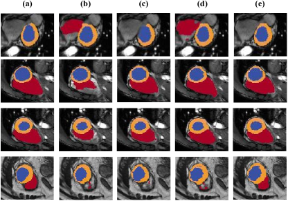
Fig. 3 gives some qualitative results, our method effectively suppresses areas that are inaccurately segmented by Cross Teaching and BCP, while accurately segmenting the foregrounds that are ignored by the two methods.
PROMISE12 dataset: Following SS-Net [37], we conduct experiments with 20% labeled data. We compare ABD with CCT [25], URPC [22], SS-Net [37], SLC-Net [20] and SCP-Net [44]. As shown in Table 2, Ours-ABD surpasses all other approaches. Compared to the recently proposed SCP-Net, ABD brings a 5.0% DSC increase.
4.4 Ablation Studies
We select Cross Teaching [23] as the baseline. All experiments are conducted on the ACDC dataset with 10% labeled data unless otherwise stated.
Effectiveness of each module in ABD: Table 3 demonstrates the effectiveness of each module in ABD by progressively adding ABD-R and ABD-I. It can be observed that the introduction of input perturbation (IP) decreases the performance of the baseline, indicating that the mixed perturbation easily leads to out-of-control. Incorporating ABD-R and ABD-I brings increased performance. By incorporating both ABD-R and ABD-I into the baseline, the model has the best result, reaching 88.52% DSC and surpassing the baseline in 2.07%. The improvement indicates that the two modules are complementary which is consistent with the design targets. ABD-R enhances the upper limit of consistency learning for mixed perturbations, and ABD-I enables the model to learn potentially uncontrollable regions, thereby the combination can learn more semantics.
Base IP ABD-R ABD-I DSC Jaccard 95HD ASD ✓ 86.45 77.02 6.30 1.86 ✓ ✓ 86.25 76.69 5.44 1.72 ✓ ✓ ✓ 87.42 78.37 5.23 1.68 ✓ ✓ ✓ 87.20 78.07 6.06 1.96 ✓ ✓ ✓ ✓ 88.52 79.97 5.06 1.43
Displacement Strategies: Table 4 illustrates the impact of different displacement strategies. The default displacement strategy (denoted as “Reliable”) in our ABD-R module is displacing the region with the top-highest confidence from one image with the region of lowest confidence from the other image. “Random” refers to randomly selecting patches for displacement. “Same” means the displacement strategy is performed by displacing the region that has the highest confidence from one image with the corresponding region from the other image. “Same+Reliable” represents that in each iteration, we randomly select a strategy from the “Same” or “Reliable”. The “Same” generates samples that have more uncontrolled regions and yields unsatisfactory results. While the “Same+Reliable” alleviates the unfavorable results, it is still not as effective as our approach.
| Strategy | DSC | Jaccard | 95HD | ASD |
|---|---|---|---|---|
| Random | 86.55 | 77.07 | 6.13 | 1.74 |
| Same | 87.22 | 78.04 | 5.61 | 1.50 |
| Same+Reliable | 87.38 | 78.06 | 4.56 | 1.69 |
| Reliable | 87.42 | 78.37 | 5.23 | 1.68 |
Selection of Patch Number: Table 5 indicates the impact of the patch number. represents the number of patches. An optimal result is achieved when .
| DSC | Jaccard | 95HD | ASD | |
|---|---|---|---|---|
| 4 | 87.39 | 78.35 | 5.06 | 1.69 |
| 16 | 88.52 | 79.97 | 5.06 | 1.43 |
| 64 | 87.54 | 78.57 | 5.52 | 1.88 |
Choice of Strong Augmentation: Table 6 illustrates the influence of three different augmentation methods: colorjitter, blur, and cutout. Through comparison, combining colorjitter and cutout produces better performance.
Cutout Colorjitter Blur DSC Jaccard 95HD ASD ✓ 88.23 79.53 5.90 1.40 ✓ 88.03 79.34 7.15 1.76 ✓ 87.76 78.76 7.28 1.61 ✓ ✓ 88.52 79.97 5.06 1.43 ✓ ✓ ✓ 87.83 79.02 6.14 1.87
5 Conclusion
In this paper, we proposed an adaptive bidirectional displacement (ABD) for semi-supervised medical image segmentation. Our key idea is to mitigate the constraints of mixed perturbations on consistency learning, thereby enhancing the upper limit of consistency learning. To achieve this, we designed two novel modules in our ABD: an ABD-R module reduces the uncontrolled regions in unlabeled samples and captures comprehensive semantic information from input perturbations, and an ABD-I module enhances the learning capacity to uncontrollable regions in labeled samples to compensate for the deficiencies of ABD-R. With the cooperation of two modules, our method achieves state-of-the-art performance and is easily embedded into different methods. In the future, we will design a patch adaptive displacement strategy to tackle more complicated cases.
Acknowledge: This work was supported by National Natural Science Foundation of China (No. 62301613), the Taishan Scholar Program of Shandong (No. tsqn202306130), the Shandong Natural Science Foundation (No. ZR2023QF046), Qingdao Postdoctoral Applied Research Project (No. QDBSH20230102091) and Independent Innovation Research Project of China University of Petroleum (East China) (No. 22CX06060A).
References
- Bai et al. [2017] Wenjia Bai, Ozan Oktay, Matthew Sinclair, Hideaki Suzuki, Martin Rajchl, Giacomo Tarroni, Ben Glocker, Andrew King, Paul M Matthews, and Daniel Rueckert. Semi-supervised learning for network-based cardiac mr image segmentation. In Medical Image Computing and Computer-Assisted Intervention, pages 253–260. Springer, 2017.
- Bai et al. [2023] Yunhao Bai, Duowen Chen, Qingli Li, Wei Shen, and Yan Wang. Bidirectional copy-paste for semi-supervised medical image segmentation. In Proceedings of the IEEE/CVF Conference on Computer Vision and Pattern Recognition, pages 11514–11524, 2023.
- Basak and Yin [2023] Hritam Basak and Zhaozheng Yin. Pseudo-label guided contrastive learning for semi-supervised medical image segmentation. In Proceedings of the IEEE/CVF Conference on Computer Vision and Pattern Recognition, pages 19786–19797, 2023.
- Bernard et al. [2018] Olivier Bernard, Alain Lalande, Clement Zotti, Frederick Cervenansky, Xin Yang, Pheng-Ann Heng, Irem Cetin, Karim Lekadir, Oscar Camara, Miguel Angel Gonzalez Ballester, et al. Deep learning techniques for automatic mri cardiac multi-structures segmentation and diagnosis: is the problem solved? IEEE transactions on medical imaging, 37(11):2514–2525, 2018.
- Berthelot et al. [2019] David Berthelot, Nicholas Carlini, Ian Goodfellow, Nicolas Papernot, Avital Oliver, and Colin A Raffel. Mixmatch: A holistic approach to semi-supervised learning. Advances in neural information processing systems, 32, 2019.
- Cao et al. [2022] Hu Cao, Yueyue Wang, Joy Chen, Dongsheng Jiang, Xiaopeng Zhang, Qi Tian, and Manning Wang. Swin-unet: Unet-like pure transformer for medical image segmentation. In European conference on computer vision, pages 205–218. Springer, 2022.
- Chen et al. [2020] Xinlei Chen, Haoqi Fan, Ross Girshick, and Kaiming He. Improved baselines with momentum contrastive learning. arXiv preprint arXiv:2003.04297, 2020.
- Chen et al. [2021] Xiaokang Chen, Yuhui Yuan, Gang Zeng, and Jingdong Wang. Semi-supervised semantic segmentation with cross pseudo supervision. In Proceedings of the IEEE/CVF Conference on Computer Vision and Pattern Recognition, pages 2613–2622, 2021.
- Du et al. [2023] Jie Du, Xiaoci Zhang, Peng Liu, and Tianfu Wang. Coarse-refined consistency learning using pixel-level features for semi-supervised medical image segmentation. IEEE Journal of Biomedical and Health Informatics, 2023.
- He et al. [2022] Wanwei He, Yinpei Dai, Yinhe Zheng, Yuchuan Wu, Zheng Cao, Dermot Liu, Peng Jiang, Min Yang, Fei Huang, Luo Si, et al. Galaxy: A generative pre-trained model for task-oriented dialog with semi-supervised learning and explicit policy injection. In Proceedings of the AAAI conference on artificial intelligence, number 10, pages 10749–10757, 2022.
- Huang et al. [2022] Wei Huang, Chang Chen, Zhiwei Xiong, Yueyi Zhang, Xuejin Chen, Xiaoyan Sun, and Feng Wu. Semi-supervised neuron segmentation via reinforced consistency learning. IEEE Transactions on Medical Imaging, 41(11):3016–3028, 2022.
- Jiao et al. [2022] Rushi Jiao, Yichi Zhang, Le Ding, Rong Cai, and Jicong Zhang. Learning with limited annotations: a survey on deep semi-supervised learning for medical image segmentation. arXiv preprint arXiv:2207.14191, 2022.
- Ke et al. [2020] Zhanghan Ke, Di Qiu, Kaican Li, Qiong Yan, and Rynson WH Lau. Guided collaborative training for pixel-wise semi-supervised learning. In Computer Vision–ECCV, pages 429–445. Springer, 2020.
- Kullback and Leibler [1951] Solomon Kullback and Richard A Leibler. On information and sufficiency. The annals of mathematical statistics, 22(1):79–86, 1951.
- Lai et al. [2021] Xin Lai, Zhuotao Tian, Li Jiang, Shu Liu, Hengshuang Zhao, Liwei Wang, and Jiaya Jia. Semi-supervised semantic segmentation with directional context-aware consistency. In Proceedings of the IEEE/CVF Conference on Computer Vision and Pattern Recognition, pages 1205–1214, 2021.
- Li et al. [2020] Xiaomeng Li, Lequan Yu, Hao Chen, Chi-Wing Fu, Lei Xing, and Pheng-Ann Heng. Transformation-consistent self-ensembling model for semisupervised medical image segmentation. IEEE Transactions on Neural Networks and Learning Systems, 32(2):523–534, 2020.
- Li et al. [2021] Yanwen Li, Luyang Luo, Huangjing Lin, Hao Chen, and Pheng-Ann Heng. Dual-consistency semi-supervised learning with uncertainty quantification for covid-19 lesion segmentation from ct images. In Medical Image Computing and Computer Assisted Intervention, pages 199–209. Springer, 2021.
- Liang et al. [2023] Chen Liang, Wenguan Wang, Jiaxu Miao, and Yi Yang. Logic-induced diagnostic reasoning for semi-supervised semantic segmentation. In Proceedings of the IEEE/CVF International Conference on Computer Vision, pages 16197–16208, 2023.
- Litjens et al. [2014] Geert Litjens, Robert Toth, Wendy Van De Ven, Caroline Hoeks, Sjoerd Kerkstra, Bram Van Ginneken, Graham Vincent, Gwenael Guillard, Neil Birbeck, Jindang Zhang, et al. Evaluation of prostate segmentation algorithms for mri: the promise12 challenge. Medical image analysis, 18(2):359–373, 2014.
- Liu et al. [2022] Jinhua Liu, Christian Desrosiers, and Yuanfeng Zhou. Semi-supervised medical image segmentation using cross-model pseudo-supervision with shape awareness and local context constraints. In International Conference on Medical Image Computing and Computer-Assisted Intervention, pages 140–150. Springer, 2022.
- Luo et al. [2021a] Xiangde Luo, Jieneng Chen, Tao Song, and Guotai Wang. Semi-supervised medical image segmentation through dual-task consistency. In Proceedings of the AAAI conference on artificial intelligence, number 10, pages 8801–8809, 2021a.
- Luo et al. [2021b] Xiangde Luo, Wenjun Liao, Jieneng Chen, Tao Song, Yinan Chen, Shichuan Zhang, Nianyong Chen, Guotai Wang, and Shaoting Zhang. Efficient semi-supervised gross target volume of nasopharyngeal carcinoma segmentation via uncertainty rectified pyramid consistency. In Medical Image Computing and Computer Assisted Intervention, pages 318–329. Springer, 2021b.
- Luo et al. [2022] Xiangde Luo, Minhao Hu, Tao Song, Guotai Wang, and Shaoting Zhang. Semi-supervised medical image segmentation via cross teaching between cnn and transformer. In International Conference on Medical Imaging with Deep Learning, pages 820–833. PMLR, 2022.
- Milletari et al. [2016] Fausto Milletari, Nassir Navab, and Seyed-Ahmad Ahmadi. V-net: Fully convolutional neural networks for volumetric medical image segmentation. In 2016 fourth international conference on 3D vision (3DV), pages 565–571. Ieee, 2016.
- Ouali et al. [2020] Yassine Ouali, Céline Hudelot, and Myriam Tami. Semi-supervised semantic segmentation with cross-consistency training. In Proceedings of the IEEE/CVF Conference on Computer Vision and Pattern Recognition, pages 12674–12684, 2020.
- Ren et al. [2023] Pengzhen Ren, Changlin Li, Hang Xu, Yi Zhu, Guangrun Wang, Jianzhuang Liu, Xiaojun Chang, and Xiaodan Liang. Viewco: Discovering text-supervised segmentation masks via multi-view semantic consistency. arXiv preprint arXiv:2302.10307, 2023.
- Ronneberger et al. [2015] Olaf Ronneberger, Philipp Fischer, and Thomas Brox. U-net: Convolutional networks for biomedical image segmentation. In Medical Image Computing and Computer-Assisted Intervention, pages 234–241. Springer, 2015.
- Sedai et al. [2019] Suman Sedai, Bhavna Antony, Ravneet Rai, Katie Jones, Hiroshi Ishikawa, Joel Schuman, Wollstein Gadi, and Rahil Garnavi. Uncertainty guided semi-supervised segmentation of retinal layers in oct images. In Medical Image Computing and Computer Assisted Intervention, pages 282–290. Springer, 2019.
- Shu et al. [2022] Yucheng Shu, Hengbo Li, Bin Xiao, Xiuli Bi, and Weisheng Li. Cross-mix monitoring for medical image segmentation with limited supervision. IEEE Transactions on Multimedia, 2022.
- Sohn et al. [2020] Kihyuk Sohn, David Berthelot, Nicholas Carlini, Zizhao Zhang, Han Zhang, Colin A Raffel, Ekin Dogus Cubuk, Alexey Kurakin, and Chun-Liang Li. Fixmatch: Simplifying semi-supervised learning with consistency and confidence. Advances in neural information processing systems, 33:596–608, 2020.
- Tajbakhsh et al. [2020] Nima Tajbakhsh, Laura Jeyaseelan, Qian Li, Jeffrey N Chiang, Zhihao Wu, and Xiaowei Ding. Embracing imperfect datasets: A review of deep learning solutions for medical image segmentation. Medical Image Analysis, 63:101693, 2020.
- Tarvainen and Valpola [2017] Antti Tarvainen and Harri Valpola. Mean teachers are better role models: Weight-averaged consistency targets improve semi-supervised deep learning results. Advances in neural information processing systems, 30, 2017.
- Verma et al. [2022] Vikas Verma, Kenji Kawaguchi, Alex Lamb, Juho Kannala, Arno Solin, Yoshua Bengio, and David Lopez-Paz. Interpolation consistency training for semi-supervised learning. Neural Networks, 145:90–106, 2022.
- Wang et al. [2019] Yan Wang, Yuyin Zhou, Wei Shen, Seyoun Park, Elliot K Fishman, and Alan L Yuille. Abdominal multi-organ segmentation with organ-attention networks and statistical fusion. Medical image analysis, 55:88–102, 2019.
- Wu et al. [2022a] Huisi Wu, Zhaoze Wang, Youyi Song, Lin Yang, and Jing Qin. Cross-patch dense contrastive learning for semi-supervised segmentation of cellular nuclei in histopathologic images. In Proceedings of the IEEE/CVF Conference on Computer Vision and Pattern Recognition, pages 11666–11675, 2022a.
- Wu et al. [2021] Yicheng Wu, Minfeng Xu, Zongyuan Ge, Jianfei Cai, and Lei Zhang. Semi-supervised left atrium segmentation with mutual consistency training. In Medical Image Computing and Computer Assisted Intervention, pages 297–306. Springer, 2021.
- Wu et al. [2022b] Yicheng Wu, Zhonghua Wu, Qianyi Wu, Zongyuan Ge, and Jianfei Cai. Exploring smoothness and class-separation for semi-supervised medical image segmentation. In International Conference on Medical Image Computing and Computer-Assisted Intervention, pages 34–43. Springer, 2022b.
- Xu et al. [2022] Mou-Cheng Xu, Yu-Kun Zhou, Chen Jin, Stefano B Blumberg, Frederick J Wilson, Marius deGroot, Daniel C Alexander, Neil P Oxtoby, and Joseph Jacob. Learning morphological feature perturbations for calibrated semi-supervised segmentation. In International Conference on Medical Imaging with Deep Learning, pages 1413–1429. PMLR, 2022.
- Yang et al. [2022] Lihe Yang, Wei Zhuo, Lei Qi, Yinghuan Shi, and Yang Gao. St++: Make self-training work better for semi-supervised semantic segmentation. In Proceedings of the IEEE/CVF Conference on Computer Vision and Pattern Recognition, pages 4268–4277, 2022.
- Yang et al. [2023a] Lihe Yang, Lei Qi, Litong Feng, Wayne Zhang, and Yinghuan Shi. Revisiting weak-to-strong consistency in semi-supervised semantic segmentation. In Proceedings of the IEEE/CVF Conference on Computer Vision and Pattern Recognition, pages 7236–7246, 2023a.
- Yang et al. [2023b] Xiaosu Yang, Jiya Tian, Yaping Wan, Mingzhi Chen, Lingna Chen, and Junxi Chen. Semi-supervised medical image segmentation via cross-guidance and feature-level consistency dual regularization schemes. Medical Physics, 2023b.
- Zhang et al. [2023a] Shuo Zhang, Jiaojiao Zhang, Biao Tian, Thomas Lukasiewicz, and Zhenghua Xu. Multi-modal contrastive mutual learning and pseudo-label re-learning for semi-supervised medical image segmentation. Medical Image Analysis, 83:102656, 2023a.
- Zhang et al. [2023b] Yichi Zhang, Rushi Jiao, Qingcheng Liao, Dongyang Li, and Jicong Zhang. Uncertainty-guided mutual consistency learning for semi-supervised medical image segmentation. Artificial Intelligence in Medicine, 138:102476, 2023b.
- Zhang et al. [2023c] Zhenxi Zhang, Ran Ran, Chunna Tian, Heng Zhou, Xin Li, Fan Yang, and Zhicheng Jiao. Self-aware and cross-sample prototypical learning for semi-supervised medical image segmentation. arXiv preprint arXiv:2305.16214, 2023c.
- Zhao et al. [2023a] Xiangyu Zhao, Zengxin Qi, Sheng Wang, Qian Wang, Xuehai Wu, Ying Mao, and Lichi Zhang. Rcps: Rectified contrastive pseudo supervision for semi-supervised medical image segmentation. arXiv preprint arXiv:2301.05500, 2023a.
- Zhao et al. [2023b] Zhen Zhao, Lihe Yang, Sifan Long, Jimin Pi, Luping Zhou, and Jingdong Wang. Augmentation matters: A simple-yet-effective approach to semi-supervised semantic segmentation. In Proceedings of the IEEE/CVF Conference on Computer Vision and Pattern Recognition, pages 11350–11359, 2023b.
- Zheng et al. [2022a] Ke Zheng, Junhai Xu, and Jianguo Wei. Double noise mean teacher self-ensembling model for semi-supervised tumor segmentation. In ICASSP 2022-2022 IEEE International Conference on Acoustics, Speech and Signal Processing (ICASSP), pages 1446–1450. IEEE, 2022a.
- Zheng et al. [2022b] Mingkai Zheng, Shan You, Lang Huang, Fei Wang, Chen Qian, and Chang Xu. Simmatch: Semi-supervised learning with similarity matching. In Proceedings of the IEEE/CVF Conference on Computer Vision and Pattern Recognition, pages 14471–14481, 2022b.
- Zhou et al. [2023] Kaiyang Zhou, Chen Change Loy, and Ziwei Liu. Semi-supervised domain generalization with stochastic stylematch. International Journal of Computer Vision, pages 1–11, 2023.
- Zhou et al. [2022] Qianyu Zhou, Zhengyang Feng, Qiqi Gu, Guangliang Cheng, Xuequan Lu, Jianping Shi, and Lizhuang Ma. Uncertainty-aware consistency regularization for cross-domain semantic segmentation. Computer Vision and Image Understanding, 221:103448, 2022.
- Zou et al. [2020] Yuliang Zou, Zizhao Zhang, Han Zhang, Chun-Liang Li, Xiao Bian, Jia-Bin Huang, and Tomas Pfister. Pseudoseg: Designing pseudo labels for semantic segmentation. arXiv preprint arXiv:2010.09713, 2020.