High-Precision Positioning with Continuous Delay and Doppler Shift using AFT-MC Waveforms

Abstract

This paper explores a novel integrated localization and communication (ILAC) system using the affine Fourier transform multicarrier (AFT-MC) waveform. Specifically, we consider a multiple-input multiple-output (MIMO) AFT-MC system with ILAC and derive a continuous delay and Doppler shift channel matrix model. Based on the derived signal model, we develop a two-step algorithm with low complexity for estimating channel parameters. Furthermore, we derive the Cramér-Rao lower bound (CRLB) of location estimation as the fundamental limit of localization. Finally, we provide some insights about the AFT-MC parameters by explaining the impact of the parameters on localization performance. Simulation results demonstrate that the AFT-MC waveform is able to provide significant localization performance improvement compared to orthogonal frequency division multiplexing (OFDM) while achieving the CRLB of location estimation.

I Introduction

Integrated localization and communications (ILAC) is expected to play a key role in a multitude of applications for the beyond fifth generation (B5G) and sixth generation (6G) wireless networks [18], such as the Internet of Things (IoT), smart environments, and autonomous driving. In particular, millimeter wave (mmWave) networks can enable new applications via large-bandwidth exploitation and multiantenna processing. However, the mmwave network also face a number of challenges. Among them, the path loss is extremely severe at high carrier frequencies, which must be compensated through beamforming [5], while the key to beamforming lies in the knowledge of the location of the target.

The propagation channel is an important bridge between localization and communication. Typical location-related channel parameters include round-trip delay, angle of arrival (AoA), angle of departure (AoD), and so on. The key to obtaining these parameters lies in the design and processing of the signal in the physical layer of the ILAC system [17].

Among the existing multicarrier waveforms, conventional orthogonal frequency division multiplexing (OFDM) has been widely studied for ILAC [16]. However, OFDM is susceptible to inter-carrier interference (ICI) in high mobility environments, which leads to degradation of communication performance. An alternative strategy for designing robust ILAC waveforms is to employ chirp-based multicarrier techniques. An early scheme was the fractional Fourier transform multicarrier (FrFT-MC) waveform [2], in which the fractional Fourier transform (FrFT) is used to generate multi-chirp signals. However, the FrFT-MC waveform cannot achieve perfect orthogonality among subcarriers, leading to inevitable performance degradation.

Another idea is the affine Fourier transform multicarrier (AFT-MC) waveform [15], which utilizes the inverse affine Fourier transform (IAFT) to modulate the information symbols into a chirp domain. In [8], the authors presented a general interference analysis of the AFT-MC system and demonstrated that the AFT-MC system could efficiently reduce interference with high spectral efficiency. In [10], the authors investigated the secrecy of the waveform in both communications and ranging and demonstrated that the AFT-MC waveform is robust against eavesdropping and signal spoofing/impersonation attacks. While its advantages in interference suppression and secrecy communication have been studied, its potential advantages in high-precision positioning have not yet been explored.

In this paper, we consider a mono-static ILAC system with the AFT-MC waveform and derive a continuous delay and Doppler shift channel matrix model for channel parameter estimation. Based on the derived signal model, we develop a low complexity algorithm to support high-precision localization. The AoA estimation is first performed independently of the other parameters via multiple signal classification (MUSIC) algorithm with spatial smoothing. Then the delay and Doppler shifts are estimated iteratively with the approximate maximum likelihood method. Meanwhile, we derive the CRLB of location estimation. Specifically, we first evaluate the Fisher information matrix (FIM) of channel parameters. Subsequently, we could obtain the FIM of the position with the bijective transformation. Furthermore, we provide some insights about the AFT-MC parameters $c_{1}$ and $c_{2}$ by analyzing how they affect localization performance.

II System Model

Let us consider an ILAC system consisting of a mono-static base station (BS) and $P$ targets of interest, as shown in Fig. 1. The BS is equipped with $N_{t}$ transmit (TX) antennas and $N_{r}$ receive (RX) antennas, which are both in the form of a uniform linear array (ULA). Each target is equipped with $N_{u}$ antennas for receiving information from the BS.

In this section, we derive the AFT-MC signal model and formulate the channel parameter estimation problem. We assume that the transmit antenna array and the receive antenna array are co-located and perfectly decoupled due to the full-duplex operation [7], the received signals would not interfere with the transmitted signals, i.e., the sensing process does not hinder the communication functions. Therefore, the focus of this paper is target positioning based on the AFT-MC waveform.

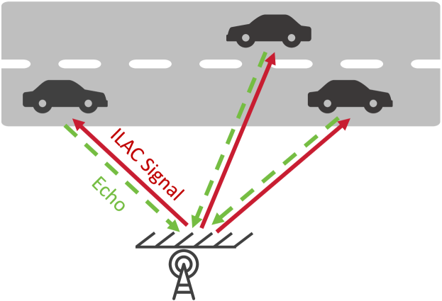
Figure 1: The considered mono-static ILAC system model.

II-A AFT-MC Transmit Signal Model

In this subsection, we briefly introduce the AFT-MC waveform proposed in [15]. Let $\mathbf{x}\in\mathbb{A}^{M\times 1}$ denote the vector of quadrature amplitude modulation (QAM) information symbols, where $M$ denotes the number of subcarriers. The transmitted baseband time domain signal is given as [15]

$$s(t)=\frac{1}{\sqrt{M}}\sum_{m=0}^{M-1}x[m]e^{j2\pi\left(c_{2}m^{2}+\frac{m}{T}t+\frac{M^{2}c_{1}}{T^{2}}t^{2}\right)},\quad 0\leq t\leq T,$$ (1)

where $T$ denotes the symbol duration, $c_{1}$ and $c_{2}$ are two adjustable AFT-MC parameters ($c_{1}$ determines the slope of the chirp subcarriers, $c_{2}$ affects the phase of the information symbol), and $x[m]$ is the $m^{th}$ element of $\mathbf{x}$.

It is then fairly easy to see that sampling at a rate of $nT/M$ for $n=0,\cdots,M-1$ results in the discrete time-domain signal as

$$s[n]=\frac{1}{\sqrt{M}}\sum_{m=0}^{M-1}x[m]e^{j2\pi\left(c_{2}m^{2}+\frac{mn}{M}+c_{1}n^{2}\right)}.$$ (2)

Equation (2) can be expressed in matrix form as

$$\mathbf{s}=\boldsymbol{\Lambda}_{c_{1}}^{H}\mathbf{F}^{H}\boldsymbol{\Lambda}_{c_{2}}^{H}\mathbf{x}=\mathbf{A}^{H}\mathbf{x},$$ (3)

where $\mathbf{A}=\boldsymbol{\Lambda}_{c_{2}}\mathbf{F}\boldsymbol{\Lambda}_{c_{1}}\in\mathbb{C}^{M\times M}$ is the M-point discrete affine Fourier transform (DAFT) matrix with the M-point unitary discrete Fourier transform (DFT) matrix $\mathbf{F}$, and $\boldsymbol{\Lambda}_{c}=\operatorname{diag}(e^{-j2\pi cm^{2}},m=0,1,\ldots,M-1)$. In this paper, The notation $(\cdot)^{{T}}$, $(\cdot)^{{*}}$ and $(\cdot)^{{H}}$ stand for transpose, conjugate and Hermitian transpose of a matrix/vector. Similar to OFDM, the transmit signal $\mathbf{s}$ need to append with a chirp periodic prefix (CPP) [9]. The signal being added CPP of length $L$ is expressed as

$$\mathbf{s}_{\mathrm{cpp}}=\left[\begin{array}[]{cc}\mathbf{0}_{L\times\left(M-L\right)}&\mathbf{C}_{L\times L}\\ \mathbf{I}_{M\times M}\end{array}\right]\mathbf{s},$$ (4)

where $\mathbf{C}=\operatorname{diag}(e^{-j2\pi c_{1}(M^{2}+2Ml)},l=-L,\cdots,-1)$, $\mathbf{I}_{M\times M}$ and $\mathbf{0}_{M\times N}$ represent $M\times M$ identity and $M\times N$ zero matrices, respectively. The CPP is not only the copy of its tail data but should have chirp periodicity. Finally, the entire time domain signal with CPP is denoted by

$$s_{\mathrm{cpp}}(t)=\left\{\begin{array}[]{ll}s(t),&0\leq t\leq T,\\ s(t+T)e^{-j2\pi c_{1}(T^{2}+2Tt)},&-T_{\mathrm{cpp}}\leq t<0,\end{array}\right.$$ (5)

where $T_{\mathrm{cpp}}=LT/M$ denotes the CPP duration. We assume that the CPP duration is greater than the round-trip delay of the farthest target.

Assuming a single-stream beamforming model [4], the signal $s_{\mathrm{cpp}}(t)$ is transmitted over all $N_{t}$ antennas using a beamforming vector $\mathbf{f}_{\mathrm{T}}$ can be represented as

$$x(t)=\mathbf{f}_{\mathrm{T}}s_{\mathrm{cpp}}(t).$$ (6)

where $\mathbf{f}_{\mathrm{T}}=\sqrt{\frac{p}{N_{t}}}\mathbf{a}(\tilde{\theta})$ is used to steer the transmitted signal $s_{\mathrm{cpp}}(t)$ towards the intended direction $\tilde{\theta}$ [13], $p$ denotes the allocated power and $\mathbf{a}(\tilde{\theta})$ denotes the steering vector of the TX antenna array, which is given by

$$\mathbf{a}(\tilde{\theta})=\left[1,e^{-j\frac{2\pi}{\lambda}d\sin(\tilde{\theta})},\ldots,e^{-j\frac{2\pi}{\lambda}d\left(N_{t}-1\right)\sin(\tilde{\theta})}\right]^{T},$$ (7)

where $\lambda$ and $d$ denote the signal wavelength and antenna element spacing, respectively.

II-B AFT-MC Receive Signal Model

Assuming the existence of $P$ targets in the far-field environment, we consider the both time and frequency selective MIMO channel model [13], which is given by

$$\mathbf{H}(t,\tau)=\sum_{i=1}^{P}\beta_{i}\mathbf{b}\left(\theta_{i}\right)\mathbf{a}^{\mathrm{H}}\left(\phi_{i}\right)\delta\left(\tau-\tau_{i}\right)e^{j2\pi\nu_{i}t},$$ (8)

where $\mathbf{b}(\theta)=\left[1,e^{-j\frac{2\pi}{\lambda}d\sin(\theta)},\ldots,e^{-j\frac{2\pi}{\lambda}d\left(N_{r}-1\right)\sin(\theta)}\right]^{T}$ denotes the steering vectors of the RX antenna array. The terms $\beta_{i}$, $\theta_{i}$, $\phi_{i}$, $\tau_{i}$ and $\nu_{i}$ denote the reflection coefficient, the AoA, the AoD, the round-trip delay, and the round-trip Doppler shift corresponding to the $i^{th}$ target, respectively. It should be noted that the AoA and AoD are assumed to have the same value as the TX and RX antenna arrays are co-located. As a result, the received signal at the BS can be expressed as

$$\mathbf{r}(t) =\sum_{i=1}^{P}\beta_{i}\mathbf{b}\left(\theta_{i}\right)\mathbf{a}^{\mathrm{H}}\left(\theta_{i}\right)x\left(t-\tau_{i}\right)e^{j2\pi\nu_{i}t}+\mathbf{w}(t)$$

$$=\sum_{i=1}^{P}\beta_{i}\mathbf{b}\left(\theta_{i}\right)\mathbf{a}^{\mathrm{H}}\left(\theta_{i}\right)\mathbf{f}_{\mathrm{T}}s_{\mathrm{cpp}}\left(t-\tau_{i}\right)e^{j2\pi\nu_{i}t}+\mathbf{w}(t)$$

$$=\sum_{i=1}^{P}\alpha_{i}\mathbf{b}\left(\theta_{i}\right)s_{\mathrm{cpp}}\left(t-\tau_{i}\right)e^{j2\pi\nu_{i}t}+\mathbf{w}(t),$$ (9)

where $\alpha_{i}\triangleq\beta_{i}\mathbf{a}^{\mathrm{H}}\left(\theta_{i}\right)\mathbf{f}_{\mathrm{T}}$, and $\mathbf{w}(t)$ stands for the additive white Gaussian noise (AWGN).

Let $s_{\tau_{i}}[n]$ denotes the sampling signal of $s_{\mathrm{cpp}}\left(t-\tau_{i}\right)$ at $t=nT/M$ for $n=0,\cdots,M-1$, we obtain

$$s_{\tau_{i}}[n] =\frac{1}{\sqrt{M}}\sum_{m=0}^{M-1}x[m]e^{j2\pi\left(c_{2}m^{2}+\frac{m}{T}\left(\frac{nT}{M}-\tau_{i}\right)+\frac{M^{2}c_{1}}{T^{2}}\left(\frac{nT}{M}-\tau_{i}\right)^{2}\right)}$$ (10)

$$=\frac{\gamma_{i}}{\sqrt{M}}\sum_{m=0}^{M-1}x[m]e^{j2\pi\left(c_{2}m^{2}+\frac{mn}{M}-\frac{m\tau_{i}}{T}+c_{1}n^{2}+\frac{2Mc_{1}n\tau_{i}}{T}\right)},$$

where $\gamma_{i}=e^{j2\pi\frac{c_{1}M^{2}{\tau_{i}}^{2}}{T^{2}}}$. Then we can derive it in the compact matrix form as

$$\mathbf{s}_{\tau_{i}} =\gamma_{i}\mathbf{c}(\tau_{i})\boldsymbol{\Lambda}_{c_{1}}^{H}\mathbf{F}^{H}\mathbf{d}(\tau_{i})\boldsymbol{\Lambda}_{c_{2}}^{H}\mathbf{x}$$

$$=\gamma_{i}\mathbf{c}(\tau_{i})\boldsymbol{\Lambda}_{c_{1}}^{H}\mathbf{F}^{H}\mathbf{d}(\tau_{i})\mathbf{F}\boldsymbol{\Lambda}_{c_{1}}\mathbf{s},$$ (11)

where $\mathbf{c}(\tau_{i})=\operatorname{diag}\{1,e^{-j2\pi\frac{2Mc_{1}\tau_{i}}{T}},\cdots,e^{-j2\pi(M-1)\frac{2Mc_{1}\tau_{i}}{T}}\}$ and $\mathbf{d}(\tau_{i})=\operatorname{diag}\{1,e^{-j2\pi\frac{\tau_{i}}{T}},\cdots,e^{-j2\pi(M-1)\frac{\tau_{i}}{T}}\}$. Finally, we can derive the input-output relation for discrete-time representation as

$$\mathbf{R} =\sum_{i=1}^{P}\alpha_{i}\mathbf{\Delta}\left(\nu_{k}\right)\mathbf{s}_{\tau_{i}}\mathbf{b}^{T}\left(\theta_{i}\right)+\mathbf{W}$$ (12)

$$=\sum_{i=1}^{P}h_{i}\mathbf{\Delta}\left(\nu_{k}\right)\mathbf{c}(\tau_{i})\boldsymbol{\Lambda}_{c_{1}}^{H}\mathbf{F}^{H}\mathbf{d}(\tau_{i})\mathbf{F}\boldsymbol{\Lambda}_{c_{1}}\mathbf{s}\mathbf{b}^{T}\left(\theta_{i}\right)+\mathbf{W},$$

where $\mathbf{\Delta}\left(\nu_{k}\right)=\operatorname{diag}\{1,e^{-j2\pi\frac{\nu_{i}}{MT}},\cdots,e^{-j2\pi(M-1)\frac{\nu_{i}}{MT}}\}$ denotes the diagonal Doppler matrix, $h_{i}=\alpha_{i}\gamma_{i}$ denotes channel gain. $\mathbf{W}$ is the additive noise matrix with $\operatorname{vec}(\mathbf{W})\sim\mathcal{CN}\left(\mathbf{0},\sigma^{2}\mathbf{I}\right)$.

By applying the discrete affine Fourier transform (DAFT), we get the demodulated AFT-MC signal as follows

$$\mathbf{Y} =\boldsymbol{\Lambda}_{c_{2}}\mathbf{F}\boldsymbol{\Lambda}_{c_{1}}\mathbf{R}$$

$$=\sum_{i=1}^{P}h_{i}\boldsymbol{\Lambda}_{c_{2}}\mathbf{F}\mathbf{\Delta}\left(\nu_{k}\right)\mathbf{c}(\tau_{i})\mathbf{F}^{H}\mathbf{d}(\tau_{i})\boldsymbol{\Lambda}_{c_{2}}^{H}\mathbf{x}\mathbf{b}^{T}\left(\theta_{i}\right)+\widetilde{\mathbf{W}}$$

$$=\sum_{i=1}^{P}h_{i}\mathbf{H}_{i}\mathbf{x}\mathbf{b}^{T}\left(\theta_{i}\right)+\widetilde{\mathbf{W}},$$ (13)

where $\mathbf{H}_{i}=\boldsymbol{\Lambda}_{c_{2}}\mathbf{F}\mathbf{\Delta}\left(\nu_{k}\right)\mathbf{c}(\tau_{i})\mathbf{F}^{H}\mathbf{d}(\tau_{i})\boldsymbol{\Lambda}_{c_{2}}^{H}$, and the noise matrix $\widetilde{\mathbf{W}}=\boldsymbol{\Lambda}_{c_{2}}\mathbf{F}\boldsymbol{\Lambda}_{c_{1}}\mathbf{W}$. Since $\boldsymbol{\Lambda}_{c_{2}}\mathbf{F}\boldsymbol{\Lambda}_{c_{1}}$ is a unitary matrix, $\widetilde{\mathbf{W}}$ and $\mathbf{W}$ have the same covariance [9].

II-C Maximum Likelihood Estimation of Channel Parameters

With full knowledge of the transmit signal $\mathbf{x}$ at the BS, it is possible to accurately estimate the channel parameters $(\boldsymbol{h},\boldsymbol{\theta},\boldsymbol{\tau},\boldsymbol{\nu})$, where $\boldsymbol{h}=[h_{1},\cdots,h_{P}]^{T}$, $\boldsymbol{\theta}=[\theta_{1},\cdots,\theta_{P}]^{T}$, $\boldsymbol{\tau}=[\tau_{1},\cdots,\tau_{P}]^{T}$, $\boldsymbol{\nu}=[\nu_{1},\cdots,\nu_{P}]^{T}$. Based on the above AFT-MC receive signal model in Sec. II-B, we formulate the problem of channel parameter estimation as a maximum likelihood estimation (MLE) problem, which is given by

$$(\hat{\boldsymbol{h}},\hat{\boldsymbol{\theta}},\hat{\boldsymbol{\tau}},\hat{\boldsymbol{\nu}})=\arg\min_{(\boldsymbol{h},\boldsymbol{\theta},\boldsymbol{\tau},\boldsymbol{\nu})}\left\|\sum_{i=1}^{P}h_{i}\mathbf{H}_{i}\mathbf{x}\mathbf{b}^{T}\left(\theta_{i}\right)-\mathbf{Y}\right\|_{F}^{2},$$ (14)

where $\left\|\cdot\right\|_{F}$ represents the Frobenius norm of a matrix.

III Channel Parameter Estimation and Localization

Note that the above channel parameter estimation problem in Sec. II-C is non-linear, and no closed-form solution exists. Moreover, a brute-force search for the 5P-dimensional (the channel gain $h_{i}$ consists of amplitude $\left|h_{i}\right|$ and phase $\angle h_{i}$) continuous domain requires high complexity and becomes unfeasible in general. To this end, we propose a channel parameter estimation algorithm with low complexity.

III-A AoA Estimation via MUSIC with Spatial Smoothing

Equation (13) implies that the AoA is decoupled from the delay-Doppler, which makes it possible to estimate the AoA independently of delay-Doppler [4]. Nevertheless, the received signal inevitably exhibit coherent signals as a result of multipath effects. For this reason, we consider the MUSIC algorithm with spatial smoothing for high-resolution AoA estimation [6]. As shown in Fig. 2, the antenna array is divided into a number of subarrays (assuming the subarray number is $K$, each subarray contains $L=M-K+1$ antennas), and the spatially smoothed signal is the average of all subarray signals. We construct the correlation matrix $\mathbf{R}_{ss}\in\mathbb{C}^{L\times L}$ of the spatially smoothed signal as

$$\mathbf{R}_{ss} =\frac{1}{K}\sum_{k=1}^{K}\mathbf{R}_{l}$$

$$=\frac{1}{KM}\sum_{k=1}^{K}\sum_{m=0}^{M-1}{\mathbf{Y}_{l}}^{H}{\mathbf{Y}_{l}},$$ (15)

where $\mathbf{Y}_{l}\in\mathbb{C}^{M\times L}$ represents the received signal of the $l^{th}$ subarray, and $\mathbf{R}_{l}\in\mathbb{C}^{L\times L}$ is the correlation matrix of $\mathbf{Y}_{l}$.

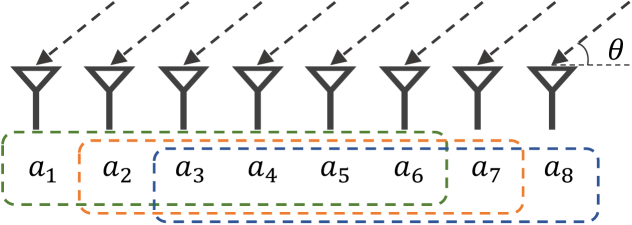
Figure 2: Principle of AoA estimation with spatial smoothing, the ULA consisting of 8 antennas is divided into 3 groups of subarrays.

Assuming $L>P$, the correlation matrix $\mathbf{R}_{ss}$ can be denoted as $\mathbf{R}_{ss}=\mathbf{U}_{s}\boldsymbol{\Lambda}_{s}\mathbf{U}_{s}^{H}+\mathbf{U}_{n}\boldsymbol{\Lambda}_{n}\mathbf{U}_{n}^{H}$, where the diagonal matrix $\boldsymbol{\Lambda}_{n}$ contains the smallest $L-P$ eigenvalues and $\boldsymbol{\Lambda}_{s}$ contains the remaining $P$ eigenvalues, corresponding to the noise and the signals respectively. The noise subspace $\mathbf{U}_{n}$ and the signal subspace $\mathbf{U}_{s}$ are orthogonal, and the MUSIC spectrum can be computed as

$$\boldsymbol{P}(\theta)=\frac{1}{\mathbf{b}^{T}(\theta)\mathbf{U}_{n}\mathbf{U}_{n}^{H}\mathbf{b}^{*}(\theta)},$$ (16)

in which sharp peaks occur at the AoA of the echo signals.

III-B Delay and Doppler Shift Estimation via Approximate Maximum Likelihood

In this subsection, we adopt an interference cancellation mechanism to estimate the delay-Doppler for multiple targets. Specifically, we first estimate the strongest signal and then subtract it from the mixed signals. Subsequently, we estimate the next strongest signal with the same process until all targets are estimated.

We reformulate the model of the received signal in equation (13) as a vector form

$$\mathbf{y}=\operatorname{vec}(\mathbf{Y})=\sum_{i=1}^{P}h_{i}\mathbf{b}\left(\theta_{i}\right)\otimes\mathbf{H}_{i}\mathbf{x}+\mathbf{w},$$ (17)

where the notation $\otimes$ represents the Kronecker product of matrices. For the $i^{th}$ target at a given angle $\hat{\theta}_{i}$, the estimator is given by

$$\left(\hat{h}_{i},\hat{\tau}_{i},\hat{\nu}_{i}\right)=\arg\min_{\left(h_{i},\tau_{i},\nu_{i}\right)}\left\|h_{i}\mathbf{b}(\hat{\theta}_{i})\otimes\mathbf{H}_{i}\mathbf{x}-\mathbf{y}_{i}\right\|_{F}^{2},$$ (18)

where $\mathbf{y}_{i}=\mathbf{y}-\sum_{j\neq i}\hat{h}_{j}\mathbf{b}(\hat{\theta}_{j})\otimes\mathbf{H}_{j}\mathbf{x}$ denotes the signal after eliminating the interference. Let $\mathbf{D}_{i}=\mathbf{b}(\hat{\theta}_{i})\otimes\mathbf{H}_{i}\mathbf{x}$, $\mathbf{D}=[\mathbf{D}_{1},\cdots,\mathbf{D}_{P}]$, for fixed $\theta_{i}$, $\tau_{i}$ and $\nu_{i}$, minimizing (18) with respect to $h_{i}$ yields

$$\hat{{h}}_{i}=\left({\mathbf{D}_{i}}^{H}{\mathbf{D}_{i}}\right)^{-1}{\mathbf{D}_{i}}^{H}{\mathbf{y}_{i}}.$$ (19)

Substituting equation (19) into (18), the minimization problem can be converted to a maximization problem as

$$\left(\hat{\tau}_{i},\hat{\nu}_{i}\right)=\arg\max_{\left(\tau_{i},\nu_{i}\right)}\left|\left(\mathbf{b}(\hat{\theta}_{i})\otimes\mathbf{H}_{i}\mathbf{x}\right)^{H}\mathbf{y}_{i}\right|^{2}.$$ (20)

The primary cause of the inaccuracy arises from inaccurate determination of background noise during the sequential estimation of delay-Doppler for each target. For example, When the algorithm estimates the delay-Doppler of the first target, it considers the residual signal (i.e., the received signal minus the first target echo) as the noise. On the contrary, the residual signal actually consists of echoes from other targets and the actual noise. Therefore, by conducting the algorithm iteratively and using the residual signal from the previous estimation as a representation of noise, we can more gradually obtain the actual noise and hence the estimated delay-Doppler can be further refined. Simulation results show that the iterative procedure can achieve satisfactory performance in only a few iterations.

The proposed channel parameter estimation algorithm is summarized in Algorithm 1.

Algorithm 1 Channel Parameter Estimation Algorithm

0:  Received signal $\mathbf{Y}$, transmitted signal $\mathbf{x}$.

0:  Channel parameter estimates of multiple targets $(\hat{\boldsymbol{h}},\hat{\boldsymbol{\theta}},\hat{\boldsymbol{\tau}},\hat{\boldsymbol{\nu}})$.

1:  Initialize $(\hat{\boldsymbol{h}},\hat{\boldsymbol{\theta}},\hat{\boldsymbol{\tau}},\hat{\boldsymbol{\nu}})=\mathbf{0}$.

2:  Executing the MUSIC algorithm with spatial smoothing to obtain the estimated AoAs $\widehat{\boldsymbol{\theta}}$.

3:  repeat

4:     for $i=1:P$ do

5:        Solve (20) and obtain delays $\widehat{\tau}_{i}$ and Doppler shift $\widehat{\nu}_{i}$.

6:        Calculate channel gains $h_{i}$ according to (19).

7:     end for

8:  until Stopping criteria.

III-C Localization Performance Analysis

With the AoA and delay estimation of all targets relative to the BS in hand, we can calculate the location of the target. Assuming that the BS is located at $\mathbf{q}_{\mathrm{BS}}=[q_{x,\mathrm{BS}},q_{y,\mathrm{BS}}]^{\mathrm{T}}$, then the location of the $i^{th}$ target $\mathbf{q}_{i}=[q_{i,x},q_{i,y}]^{\mathrm{T}}$ can be calculated as

$$\hat{q}_{i,x}=q_{x,\mathrm{BS}}+\frac{c_{0}\hat{\tau}_{i}\sin\hat{\theta}_{i}}{2},\quad\hat{q}_{i,y}=q_{y,\mathrm{BS}}+\frac{c_{0}\hat{\tau}_{i}\cos\hat{\theta}_{i}}{2}.$$ (21)

where $c_{0}$ represents the speed of light.

Following, we analyze the localization performance using the CRLB of location estimation. Specifically, we first evaluate the Fisher information matrix (FIM) of channel parameters, then convert it to the FIM of location estimation, and finally the CRLB for all target positions can be calculated.

Let $\boldsymbol{\rho}=[\boldsymbol{\theta}^{T},\boldsymbol{\tau}^{T},\boldsymbol{\nu}^{T}]^{T}$ denote the channel parameter vector (in addition to the channel gain $\boldsymbol{h}$). Performing similar calculations in [11], the FIM $\mathbf{J}(\boldsymbol{\rho})\in\mathbb{C}^{3P\times 3P}$ of channel parameters is given by

$$\mathbf{J}(\boldsymbol{\rho})=\frac{2}{\sigma^{2}}\operatorname{Re}\left\{\mathbf{E}^{H}\mathbf{P}_{\mathbf{D}}^{\perp}\mathbf{E}\odot\left({\tilde{\boldsymbol{h}}}^{*}{\tilde{\boldsymbol{h}}}^{T}\right)\right\},$$ (22)

where $\tilde{\boldsymbol{h}}=[\boldsymbol{h}^{T},\boldsymbol{h}^{T},\boldsymbol{h}^{T}]^{T}$, the notation $\odot$ represents the Hadamard product of matrices, $\operatorname{Re}\{\cdot\}$ represents the real part of a complex number matrix,

$$\mathbf{E}=\left[\frac{\partial\mathbf{D}_{1}}{\partial\theta_{1}},\cdots,\frac{\partial\mathbf{D}_{P}}{\partial\theta_{P}},\frac{\partial\mathbf{D}_{1}}{\partial\tau_{1}},\cdots,\frac{\partial\mathbf{D}_{P}}{\partial\tau_{P}},\frac{\partial\mathbf{D}_{1}}{\partial\nu_{1}},\cdots,\frac{\partial\mathbf{D}_{P}}{\partial\nu_{P}}\right],$$

$\mathbf{P}_{\mathbf{D}}^{\perp}=\mathbf{I}_{M\times N_{r}}-\mathbf{D}\left(\mathbf{D}^{H}\mathbf{D}\right)^{-1}\mathbf{D}^{H}$ represents the projection matrix onto the null space of matrix $\mathbf{D}$.

Let $\boldsymbol{\eta}=[\mathbf{q}_{1}^{T},\cdots,\mathbf{q}_{P}^{T}]^{T}$ denote the location vector. By performing the bijective transformation, the FIM $\mathbf{J}(\boldsymbol{\eta})\in\mathbb{C}^{2P\times 2P}$ of position estimation can be obtained as

$$\mathbf{J}(\boldsymbol{\eta})=\mathbf{T}\mathbf{J}(\boldsymbol{\rho})\mathbf{T}^{T},$$ (23)

where

$$\mathbf{T}=\frac{\partial\boldsymbol{\rho}^{T}}{\partial\boldsymbol{\eta}}=\left[\frac{\partial\boldsymbol{\theta}^{T}}{\partial\boldsymbol{\eta}},\frac{\partial\boldsymbol{\tau}^{T}}{\partial\boldsymbol{\eta}},\frac{\partial\boldsymbol{\nu}^{T}}{\partial\boldsymbol{\eta}}\right]\in\mathbb{C}^{2P\times 3P}.$$ (24)

We finally obtain the CRLB for all target positions as

$$\operatorname{CRLB}(\boldsymbol{\eta})=\frac{\sigma^{2}}{2}\left[\operatorname{Re}\left\{\mathbf{T}\mathbf{E}^{H}\mathbf{P}_{\mathbf{D}}^{\perp}\mathbf{E}\odot\left({\tilde{\boldsymbol{h}}}^{*}{\tilde{\boldsymbol{h}}}^{T}\right)\mathbf{T}^{T}\right\}\right]^{-1}.$$ (25)

III-D AFT-MC Parameters

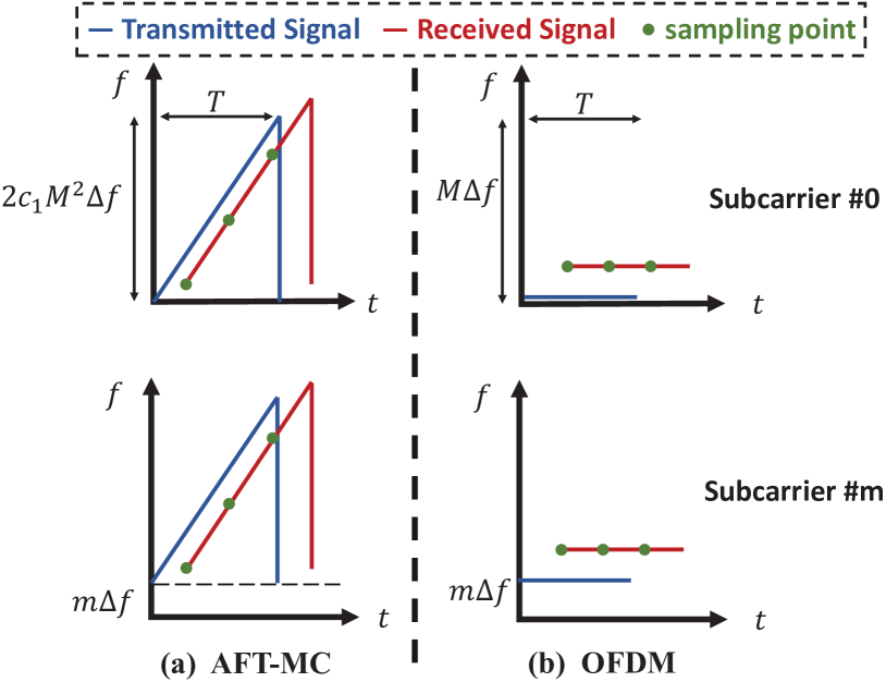
Figure 3: The illustration of the transmitted and received signals using (a) AFT-MC and (b) OFDM.

In this subsection, we show some insights about AFT-MC parameters $c_{1}$ and $c_{2}$. The channel impulse response (CIR) in time-frequency domain is given by

$$\mathbf{H}(t,f)=\sum_{i=1}^{P}\beta_{i}\mathbf{b}\left(\theta_{i}\right)\mathbf{a}^{\mathrm{H}}\left(\theta_{i}\right)e^{j2\pi\nu_{i}t}e^{-j2\pi\tau_{i}f}.$$ (26)

We can observe that the mechanism of delay estimation lies in the phase difference of $e^{-j2\pi\tau_{i}f}$. In the OFDM system, the frequency of each subcarrier over time is fixed, where $f=m\Delta f$ for $m=0,\cdots,M-1$, $\Delta f=1/T$ denotes the subcarrier spacing. The phase difference $e^{-j2\pi\tau_{i}m\Delta f}$ is only introduced between different subcarriers. However, the frequency of each chirp subcarrier changes linearly over time for the AFT-MC waveform, as shown in Fig. 3(a). The phase difference $e^{-j2\pi\tau_{i}m\Delta f}$ is not only introduced between different subcarriers but also has a phase difference $e^{-j4\pi Mc_{1}\tau_{i}n\Delta f}$ at different sampling points $nT/M$ for $n=0,\cdots,M-1$.

When the AFT-MC waveform has only one subcarrier and $2Mc_{1}=1$, it could realize similar ranging performance as OFDM. When the AFT-MC waveform has multiple subcarriers or enlarges $c_{1}$, better ranging performance can be obtained compared to OFDM.

Furthermore, the equation (25) demonstrates that the calculation of CRLB is associated with parameter $c_{2}$. In other words, with sufficient understanding of the channel characteristics (i.e., the channel parameters are known), it is possible to select the appropriate $c_{2}$ to minimize the CRLB and thus enhance the localization performance.

IV Simulation Results

In this section, we validated our proposed ILAC scheme based on AFT-MC waveforms in the mmWave channel through numerical simulations. The transmit symbols $\mathbf{x}$ are chosen randomly from a 16-QAM alphabet, and the simulation parameters are described in Table I. Mutually independent AWGN is added to control the signal-to-noise ratio (SNR). In implementing the proposed two-step channel parameter estimation algorithm, each loop in the delay-Doppler estimation is terminated after 3 iterations. We consider two reference targets as, $(50\mathrm{~{}m},50\mathrm{~{}m}/\mathrm{s}$, $30^{\circ})$, $(100\mathrm{~{}m},100\mathrm{~{}m}/\mathrm{s},50^{\circ})$. To illustrate the localization performance, each provided result is an average over 300 independent runs.

TABLE I: Simulation Parameters

Notation	Definition	Value
$f_{c}$	Carrier frequency	$60\mathrm{~{}GHz}$
$M$	Number of subcarriers	64
$\Delta f$	Subcarrier spacing	$15\mathrm{~{}KHz}$
$T$	Symbol Duration	$66.67~{}\mu\mathrm{s}$
$T_{\mathrm{cpp}}$	Chirp Cyclic Prefix Duration	$16.67~{}\mu\mathrm{s}$
$N_{t}$	Number of transmit antennas	16
$N_{r}$	Number of receive antennas	16

First, we demonstrate the localization performance with various AFT-MC parameters, as shown in Fig. 4. As $c_{1}$ increases, the CRLB of location estimation significantly decreases. Additionally, we could observe that different values of $c_{2}$ affect the localization performance as well. The results accord well with our insights in Sec. III-D.

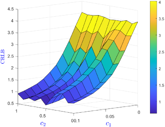
Figure 4: The CRLB of location estimation with different AFT-MC parameters.

Next, we show in Fig. 5 the performance of the AoA estimation. We compare the spatially smoothed MUSIC (SS-MUSIC) with conventional beamforming (CBF), minimum variance distortionless response (MVDR), and MUSIC. The results show the SS-MUSIC algorithm has a narrower main lobe width, which can achieve better performance.

We further investigate the localization accuracy for the AFT-MC and OFDM. The performance metrics are the root mean square error (RMSE) and CRLB. As shown in Fig. 6, the AFT-MC with $c_{1}=0.03$ significantly improves localization accuracy by an order of magnitude compared to OFDM. At the same time, as $c_{1}$ increases, there is a corresponding improvement in localization accuracy. It also validates the effectiveness of the channel parameter estimation algorithm we proposed. In Fig. 7, we consider $c_{1}=0$ and optimal $c_{2}$ (in each independent experiment, We assume that the transmit symbols $\mathbf{x}$ are fixed and the channel parameters are known, the optimal $c_{2}$ is selected by a heuristic algorithm [1] to minimize the CRLB). Simulation results show that better localization performance can be achieved by choosing a appropriate $c_{2}$.

As a final remark, although the advantages of AFT-MC come at a considerable cost in terms of signal bandwidth, it is possible to deploy the AFT-MC waveform in mmWave networks with large-bandwidth. Additionally, the severe path loss issues in mmWave networks can be mitigated by pulse compression techniques. Therefore, the AFT-MC waveform based on chirp signals can be considered a strong candidate of the ILAC-enabling waveform for B5G and 6G systems.

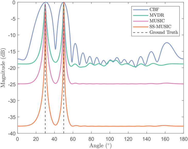
Figure 5: AoA Estimation spectrum using different algorithms.

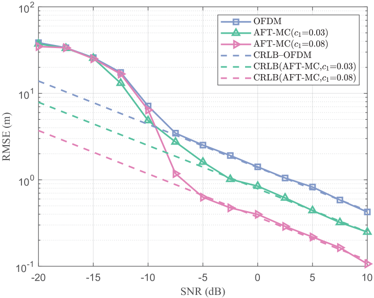
Figure 6: Localization performance comparison using OFDM, AFT-MC ($c_{1}=0.03$, $c_{2}=0$) and AFT-MC ($c_{1}=0.08$, $c_{2}=0$).

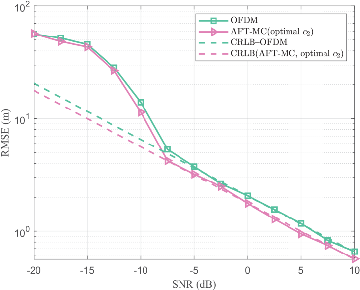
Figure 7: Localization performance comparison using OFDM and AFT-MC ($c_{1}=0$, optimal $c_{2}$).

V Conclusion

In this paper, we provide an in-depth study of the ILAC system with the AFT-MC waveform and exploit its potential advantages in high-precision localization. We derive a continuous delay and Doppler shift channel matrix model and develop a novel algorithm to support multi-target localization. The proposed algorithm first obtains the AoA of the received signal and then iteratively estimates the delay-Doppler by approximating the maximum likelihood method. The simulation results demonstrate the feasibility of the proposed algorithm and the potential of the AFT-MC waveform for high-precision localization. Our future work will be devoted to the development of a facile parameter selection strategy to realize the trade-off between localization and communication.

References

- [1] S. Mirjalili, S. M. Mirjalili, and A. Lewis, “Grey wolf optimizer,” Advances in engineering software, vol. 69, pp. 46–61, 2014.
- [2] M. Martone, “A multicarrier system based on the fractional fourier transform for time-frequency-selective channels,” IEEE Trans. Commun., vol. 49, no. 6, pp. 1011–1020, 2001.
- [3] H. Yin, X. Wei, Y. Tang, and K. Yang, “Diagonally reconstructed channel estimation for MIMO-AFDM with inter-doppler interference in doubly selective channels,” arXiv preprint arXiv:2206.12822, 2023.
- [4] M. F. Keskin, H. Wymeersch, and V. Koivunen, “MIMO-OFDM joint radar-communications: Is ICI friend or foe?” IEEE J. Sel. Areas Commun., vol. 15, no. 6, pp. 1393–1408, 2021.
- [5] S. Hur, T. Kim, D. J. Love, J. V. Krogmeier, T. A. Thomas, and A. Ghosh, “Millimeter wave beamforming for wireless backhaul and access in small cell networks,” IEEE Trans. Commun., vol. 61, no. 10, pp. 4391–4403, 2013.
- [6] S. Pillai and B. Kwon, “Forward/backward spatial smoothing techniques for coherent signal identification,” IEEE Transactions on Acoustics, Speech, and Signal Processing, vol. 37, no. 1, pp. 8–15, 1989.
- [7] P. Kumari, S. A. Vorobyov, and R. W. Heath, “Adaptive virtual waveform design for millimeter-wave joint communication–radar,” IEEE Trans. Signal Process., vol. 68, pp. 715–730, 2020.
- [8] D. Stojanović, I. Djurović, and B. R. Vojcic, “Multicarrier communications based on the affine Fourier transform in doubly-dispersive channels,” EURASIP Journal on Wireless Communications and Networking, vol. 2010, pp. 1–10, 2010.
- [9] A. Bemani, N. Ksairi, and M. Kountouris, “Affine frequency division multiplexing for next generation wireless communications,” IEEE Trans. Wireless Commun., vol. 22, no. 11, pp. 8214–8229, 2023.
- [10] Y.-G. Zhang, H.-M. Wang, P. Liu, and X.-H. Lu, “A robust joint sensing and communications waveform against eavesdropping and spoofing,” in 2022 IEEE 95th Vehicular Technology Conference, 2022, pp. 1–6.
- [11] F. Wen, P. Liu, H. Wei, Y. Zhang, and R. C. Qiu, “Joint azimuth, elevation, and delay estimation for 3-D indoor localization,” IEEE Trans. Veh. Technol., vol. 67, no. 5, pp. 4248–4261, 2018.
- [12] L. Gaudio, M. Kobayashi, G. Caire, and G. Colavolpe, “On the effectiveness of OTFS for joint radar parameter estimation and communication,” IEEE Trans. Wireless Commun., vol. 19, no. 9, pp. 5951–5965, 2020.
- [13] W. Yuan, Z. Wei, S. Li, R. Schober, and G. Caire, “Orthogonal time frequency space modulation—Part III: ISAC and potential applications,” IEEE Communications Letters, vol. 27, no. 1, pp. 14–18, 2023.
- [14] P. Kumari, J. Choi, N. González-Prelcic, and R. W. Heath, “IEEE 802.11ad-based radar: An approach to joint vehicular communication-radar system,” IEEE Trans. Veh. Technol., vol. 67, no. 4, pp. 3012–3027, 2018.
- [15] T. Erseghe, N. Laurenti, and V. Cellini, “A multicarrier architecture based upon the affine Fourier transform,” IEEE Trans. Commun., vol. 53, no. 5, pp. 853–862, 2005.
- [16] G. Kwon, Z. Liu, A. Conti, H. Park, and M. Z. Win, “Integrated localization and communication for efficient millimeter wave networks,” IEEE J. Sel. Areas Commun., vol. 41, no. 12, pp. 3925–3941, 2023.
- [17] Z. Gong, F. Jiang, C. Li, and X. Shen, “Simultaneous localization and communications with massive MIMO-OTFS,” IEEE J. Sel. Areas Commun., vol. 41, no. 12, pp. 3908–3924, 2023.
- [18] Z. Xiao and Y. Zeng, “An overview on integrated localization and communication towards 6G,” Science China Information Sciences, 2022.