Directed Redundancy in Time Series
Abstract
We quantify the average amount of redundant information that is transferred from a subset of relevant random source processes to a target process. To identify the relevant source processes, we consider those that are connected to the target process and in addition share a certain proportion of the total information causally provided to the target. Even if the relevant processes have no directed information exchange between them, they can still causally provide redundant information to the target. This makes it difficult to identify the relevant processes. To solve this issue, we propose the existence of a hidden redundancy process that governs the shared information among the relevant processes. We bound the redundancy by the minimal average directed redundancy from the relevant processes to the target, from the hidden redundancy process to the target, and from the hidden redundancy process to the relevant processes.
I INTRODUCTION
Mutual information is frequently used when quantifying the amount of redundancy between random variables [1]. Shannon’s mutual information measure is only able to quantify the shared information between two sets of variables [2]. Thus, a naive way to compute the amount of common information of three or more variables is to use the minimum of their pairwise mutual informations. Alternative ways of analyzing the intrinsic relationships between multiple random variables have been considered in e.g., [3, 4, 5, 6, 7, 8, 9, 10, 11].
Consider the case where is the target signal and and the source signals. We are interested in assessing the amount of redundant information in due to and , i.e., the amount of shared information that both and convey to . This was considered for discrete random variables in [3] as:
| (1) | ||||
where are the alphabets of , and , respectively.
An extension of the redundancy measure in (1) to continuous-alphabet sources was considered in [12]:
| (2) |
In order to extend (2) to processes, one could use a directed measure for discrete-time stationary processes and ; such as transfer entropy [13]:
| (3) |
We can then form a directed version of the average minimal redundancy measure for processes as follows:
| (4) | ||||
We are, however, facing a number of problems with (4):
-
i)
Computing for every is practically infeasible since is uncountably infinite.
-
ii)
If there are more than two source processes, the minimum would be taken over all sources processes. However, perhaps only a few of them are connected to the target, and hence the minimum transfer entropy over all source processes and to the target is then always zero.
-
iii)
A positive transfer entropy does not necessarily imply that the processes are causally related.
Note also that two source processes that have zero causal interaction with each other, could potentially still causally provide redundant information to the target.
It was suggested in [12] and further developed in [14] to use the minimum transfer entropy from the sources to the target as a measure of redundancy. Such an approach would solve problem i). Moreover, the idea that source variables can be weakly or even uncorrelated and yet carry redundant information was discussed in [5] and [12]. Here they suggested to not consider the mutual information among all the source variables but only between the sources and the target. We will leverage upon both of these ideas in the sequel.
In this paper, we propose and analyze a new notion of directed redundancy that is applicable to both discrete-time continuous-alphabet and discrete-alphabet processes. The notion is motivated by the analysis of brain networks, where it is currently unknown to what degree the human brain relies upon redundant information for processing [15].
Our main contribution is to quantify the redundant information exchange a set of relevant source processes each provide to a given target process. This is complicated by the following problem. Two causally independent sources could provide different (and hence non-redundant) information to the target. Thus, if we only measure the amount of causal information exchange from the sources and to the target, then these sources would wrongly be classified as providing redundant information transfer to the target. On the other hand, the causal information exchange between the source processes could be zero even though they provide redundant information to the target. Thus, it is necessary but non-trivial to include the dependency between the sources to guarantee that they actually provide redundant information to the target. To tackle this problem, we hypothesize the existence of a (perhaps hidden) redundancy process, , which causally affect the source processes. Thus, if we know , we can compute the causal information exchange from to all the relevant sources, and also to the target. The minimum of these causal exchanges, would be an upper bound to the redundancy.
I-A Notation
We use to denote a one-sided scalar random process, i.e., where . For brevity, we will occasionally refer to simply by . For example, denotes the transfer entropy from to .The th element of is denoted , and . We use the notation to distinguish between time-series each of length . If , for a deterministic function , then there is a directional (or causal) dependency from to .
II Redundancy via Minimal Sufficient Statistics
In this section, we motivate the use of minimal sufficient statistics as a means to bound the common information. Let , and be mutually independent discrete random variables. Moreover, let , and . What is the amount of common (redundant) information between , and ? Using the minimum of their pairwise mutual informations yields:
| (5) |
since . Similarly, and . Thus, if the entropies are positive the pairwise common information is positively bounded away from zero. On the other hand, we can define a notion of redundancy based upon sufficient statistics, which is zero for the above example. Let be a sufficient statistics of with respect to , i.e., and forms a Markov chain, i.e., and are conditionally independent of each other given knowledge of [1]. A minimal sufficient statistics satisfies [1]:
For the above example, one may observe that the minimal sufficient statistics are , and . Then, clearly . Since the minimal sufficient statistics have no information overlap with each other one could argue that the triplet therefore should have zero information in common, which implies zero redundancy. The above example inspire us to introduce a new notion of redundancy for random variables, which we extend to processes in the next section:
| (6) | ||||
where denotes a minimal sufficient statistics for with respect to , and similarly for and . Clearly,
III Directed Redundancy
In this section, we introduce a hidden redundancy process, and define a notion of directed redundancy for processes.
III-A Hidden redundancy process
The following example illustrates the usefulness of considering a (perhaps hidden) redundancy process that governs the shared information, which is exhanged by a set of source processes to a target process. Consider the following system:
| (7) | ||||
| (8) | ||||
| (9) | ||||
| (10) | ||||
| (11) |
where , are mutually independent and standard normally distributed. This set of processes is constructed such that represents a (hidden) redundancy process which "induces" redundant information exchanges to via and but not via . However, is also causally providing information to the target. Thus, if one would use a measure like (5), then the redundancy would be estimated as being zero, since is causally independent of and . Even if the mutual dependency between the sources were left out, the estimate would be the minimum of , which is also wrong, since the information provided by is independent (and hence not redundant) of that provided by to the target. Our key idea is to only focus upon the relevant source processes, and , which provide some common directed information to even though they are causally independent of each other.
III-B Directed Redundancy for Processes
In the sequel, we will consider the transfer entropy to be our desired measure of directed (causal) information exchange. Our results are also valid if the transfer entropy is substituted by, e.g., conditional directed information [16, 17].
Definition 1
The transfer-entropy measurable causal redundancy provided to the target via the source processes , which are driven by the hidden redundancy process is defined as:
where is a causal minimal sufficient statistics for with respect to , which we define to mean that satisfies the conditional Markov chain
where
The last quantity in the definition is a standard mutual information. This term is necessary to exclude the case where and would only be providing non-redundant information to in which case .
It is non-trivial to find minimal sufficient statistics for general sources, and below we introduce an upper bound to the redundancy that does not rely on minimal sufficient statistics.
Lemma 1
Proof:
The proof follows by replacing the minimal sufficient statistics in Definition 1 by their associated random processes. Omitting can only increase the estimated redundancy. may overestimate the amount of information exchanged from to , since also receives information from . Similarly for . Thus, it is necessary to also take into account the amount of redundant information that is induced into and . This is upper bounded by and , respectively. Finally, since is driving the redundancy in the system, the redundancy can be no greater than . ∎
The following lemma demonstrates the existence of systems that are bounded by the different terms in (12), and thereby showing that all of the terms are needed.
Lemma 2
Proof:
We first expand by the chain rule of mutual information:
The first term can be further written as:
Since , follows, and it further implies . Similarly, we have that:
Finally, , where:
All the arguments of the logarithms in (13), (14), and (15) are convex in , and are having their minima at and maxima at . Pairwise equating the arguments of (13), (14), and (15), and solving for , yields real roots corresponding to the cases provided in (16). The minima can then readily be verified by evaluating the arguments for any within the corresponding regions. ∎
Example 1
Let , and let the length of the processes in (7) – (11) be . The transfer entropies between all pairs of processes are shown in Table I.111The TRENTOOL transfer entropy estimator of [18] was used. It can be observed that all sources () appears to be coupled to the target , and one could therefore wrongly conclude that they all provide a degree of common (redundant) information, which would be upper bounded by . This is clearly a false assessment, since the information provided by to is distinct from that provided by to and hence and convey zero common information to . Let us now ignore and treat as the source that is driving the redundancy. An upper bound to the amount of common information which and both relay to is then via Lemma 1 estimated as .
| From/To | |||||
|---|---|---|---|---|---|
| – | 0.00 | 0.00 | 0.00 | 0.03 | |
| 0.00 | – | 0.09 | 0.09 | 0.04 | |
| 0.00 | 0.00 | – | 0.00 | 0.06 | |
| 0.00 | 0.00 | 0.00 | – | 0.06 | |
| 0.00 | 0.00 | 0.00 | 0.00 | – |
In the above example, we deliberately made the choice of omitting , and focusing on the exchange of redundant information from only via the sources and to the target . For larger systems, or for systems with unknown dynamics, it would be advantageous to use a systematic approach to select the hidden redundancy process and the associated desired set of relevant sources. In principle, one could consider all possible subsets of sources and find the one that maximizes the minimal transfer entropy among them. This is a problem with exponential complexity in the number of possible subsets, and equally important, it is known that the amount of redundant information between variables is decreasing in the number of variables [3]. Thus, such a strategy would potentially be biased towards selecting a minimal number of sources. We propose an efficient strategy for finding a hidden redundancy process and selecting its associated relevant sources in Section IV.
IV Selecting relevant source processes
In this section, we consider multiple sources and a single target . We will first identify the subset of sources that are relevant with respect to the target , i.e., we are interested in determining whether they are "causally" coupled to the target as measured by the strength of the transfer entropy from to . Then we identify the hidden process, , and finally identify the subset of relevant sources, i.e., those that are all governed by the hidden process and in addition they are all coupled to the target.
IV-A Target-relevant source processes
We propose to find a tentative set of sources, which is a set of sources that are all coupled to the target. We refer to as the target-relevant set of sources. We choose to define this set as the one with the minimal number of sources that provides at least an -fraction of the total sum of transfer entropy from all sources to the target. This is akin to the smallest high-probability sets in [19, Ch.4.3]. This can formally be stated as the following optimization problem (for ):
| (17) | ||||
The constraint in (17) provides an efficient way to omit sources that are only weakly coupled to the target. The optimization problem can be efficiently computed by first sorting the transfer entropies in descending order, and then including the greatest elements one by one until the threshold is breached. If several elements have equal probability, there could be ambiguous output unless is adjusted to either include or exclude all of the equal probability elements, cf. [19].
IV-B Identifying the hidden process
We will now find the hidden redundancy process, which is that particular source out of all the sources in , which dominates the redundancy within a selective group of relevant sources. For each source , where , find the minimal subset of that provides a given fraction of the total amount of transfer entropy:
| (18) | ||||
The minimal causal information exchange from the th source and to its associated processes in is:
| (19) |
Out of all the source processes in , the one that induces the greatest minimal redundancy within its associated set of sources will be chosen as the hidden redundancy process:
| (20) | ||||
| (21) | ||||
| (22) |
where is the hidden redundancy process, is the set of relevant sources associated with , and is an upper bound on the redundancy induced by into the set .
IV-C Bounding the minimal redundant information
Inspired by Lemma 1, we formulate the following upper bound to the causal redundancy defined by Definition 1:
Theorem 1
The minimal redundant information causally exchanged (as measured by the transfer entropy) to the target via a set of relevant sources, and which is due to a single hidden redundancy process is upper bounded by:
| (23) |
where
| (24) | ||||
| (25) |
Proof:
bounds the information exchange from the hidden redundancy process to the target, bounds the information exchange from the hidden redundancy process and to the relevant sources, and bounds the information exchange from the relevant sources to the target. ∎
V Simulation study
We consider 76-channel real-world intracranial EEG recordings obtained from a patient undergoing 8 periods of seizures. 64 cortical electrodes (referred to as electrodes 1 – 64) and 12 in-depth electrodes (referred to as electrodes 65 – 76) arranged as two 6 nodes depth-strips were implanted on the subject. Details about the data can be obtained from [20]222Data available online: http://math.bu.edu/people/kolaczyk/datasets.html. It was pointed out in [20] that in particular the depth-strip with electrodes 71 – 76 and the lower left corner of the cortical grid with electrodes 1 – 4, 9 – 11, and 17 exhibited strong synchronous neuronal activity during seizures.
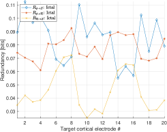
In our study, the lower range of cortical electrodes ranging from 1 – 20 will be considered the targets. The sources will be all the 12 depth electrodes and the hidden redundancy processes will also be found amongst the 12 depth electrodes. For each target electrode we first find the set of sources that are coupled to the target using (17). Then we identify the hidden redundancy process, which is inducing the majority of the redundancy in the set. This is done using (21). Having identified a potential hidden redundancy process for a given target electrode, we then use (22) to find the associated set of relevant source processes. From the target, the hidden redundancy process, and this set of relevant source processes, we can find the corresponding transfer entropies given by (24). These are plotted in Fig. 1. The parameters used for the transfer entropy estimator are: a maximum lag of 5, 10 nearest neighbors, and . A greater means less source selected.
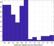
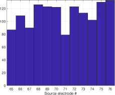
From Fig. 1 one can observe that the minimal redundancy mainly follows , i.e., the minimal transfer entropy from the relevant sources and to the targets. It is interesting to see that the minimal redundancy is peaking for target electrodes 6 – 8 and 14 – 16, which are complementary to the electrodes identified in [20] that were exhibiting strong synchronous neuronal activity. Moreover, the transfer entropy between the hidden redundancy processes and the targets reaches its minima when is peaking. This can be explained by the fact that when is high, the same information is exchanged via different sources, and thus the total information about that exists in the targets is not much greater than that provided by a single source. On the other hand, when is low, the different sources could potentially provide distinct information about to the target, which would result in an overall greater amount of information about in the targets. To further explore the cases, where the redundancy is peaking, i.e., for target electrodes 6 – 8 and 14 – 16, we have shown the histograms for the selected hidden redundancy processes, see Fig. 1 (right), and their associated relevant sources, see Fig. 2 (left). It is interesting to note from Fig. 2 (left) that the redundancy appears to mainly come from within sources on the same depth-strip (electrodes 65 – 70). Moreover, Fig. 1 (right) shows that the hidden redundancy process is also mainly belonging to this depth-strip. The most frequently chosen electrode as the hidden redundancy process is #68. This one is then selected less as a relevant source, since the hidden redundancy process is excluded when finding the relevant sources. We have tried to compare our findings with the graph theoretic analysis of the electrodes provided in [20], however, we have been unable to explain why electrode 68 appears to be the main driver of redundancy. For comparison, we have in Fig. 2 (right) shown the histogram of the sources in (17), i.e., those having 80% of the entire transfer entropy to the targets. In this case, the hidden redundancy process is not taken into account, and a more uniform distribution is obtained compared to Fig. 2, where the hidden redundancy process is taken into account.

VI Conclusions
We proposed a new methodology for quantifying the causal redundancy provided by a set of source processes (time series) to a target process. The sources do not need to be causally dependent upon each other. Instead we motivated the existence of a hidden redundancy process, which governs the redundancy within a subset of the source processes. We defined a set of relevant source processes to be those that are causally coupled to the target, and where the hidden redundancy process is causally coupled to all of them. We finally provided an upper bound for the redundancy as the minimal average redundancy from the relevant sources to the target, from the hidden redundancy process to the target, and from the hidden redundancy process to the relevant sources.
References
- [1] T. Cover and J. Thomas, Elements of Information Theory. Wiley-Interscience, 2006.
- [2] R. Yeung, “A first course in information theory,” Springer, 2002.
- [3] P. L. Williams and R. D. Beer, “Nonnegative decomposition of multivariate information,” CoRR, vol. abs/1004.2515, 2010.
- [4] M. Harder, C. Salge, and D. Polani, “Bivariate measure of redundant information,” Physical Review E, vol. 87, no. 1, 2013.
- [5] N. Bertschinger, J. Rauh, E. Olbrich, J. Jost, and N. Ay, “Quantifying unique information,” Entropy, vol. 16, p. 2161–2183, 2014.
- [6] R. A. A. Ince, “Measuring multivariate redundant information with pointwise common change in surprisal,” Entropy, vol. 19, no. 7, 2017.
- [7] R. G. James and J. P. Crutchfield., “Multivariate dependence beyond shannon information,” Entropy, 2017.
- [8] M. Wibral, V. P. J. Kay, J. Lizier, and W. Philips, “Partial information decomposition as a unified approach to the specification of neural goal functions,” Brain and Cognition, vol. 112, 2017.
- [9] J. Kunert-Graf, N. Sakhanenko, and D. Galas, “Partial information decomposition and the information delta: A geometric unification disentangling non-pairwise information,” Entropy, vol. 22, no. 1333, 2020.
- [10] R. James, J. Emenheiser, and J. Crutchfield, “Unique information and secret key agreement,” MDPI Entropy, vol. 21, no. 1, 2021.
- [11] P. Mediano, F. Rosas, A. Luppi, R. Carhart-Harris, D. Bor, A. Seth, and A. Barrett, “Towards an extended taxonomy of information dynamics via integrated information decomposition,” arxiv.org:, 2021.
- [12] A. B. Barrett, “Exploration of synergistic and redundant information sharing in static and dynamical gaussian systems,” Phys. Rev. E., vol. 91, no. 052802, 2015.
- [13] T. Schreiber, “Measuring information transfer,” Phys. Rev. Lett., vol. 85, 2000.
- [14] L. Faes, D. Marinazzo, and S. Stramaglia, “Multiscale information decomposition: Exact computation for multivariate gaussian processes,” Entropy, 2017.
- [15] A. Luppi, P. Mediano, F. Rosas, N. Holland, T. Fryer, J. O’Brien, J. Rowe, D. Menon, D.Bor, and E. Stamatakis, “A synergistic core for human brain evolution and cognition,” Nature Neuroscience, vol. 25, 2022.
- [16] J. Massey, “Causality, feedback and directed information,” The International Symposium on Information Theory and Its Applications, 1990.
- [17] G. Kramer, “Capacity results for the discrete memoryless network,” IEEE Transactions on Information Theory, vol. 49, no. 1, pp. 4–21, 2003.
- [18] M. Lindner, R. Vicente, V. Priesemann, and M. Wibral, “Trentool: a matlab open source toolbox to analyse information flow in time series data with transfer entropy,” BMC Neurosci., vol. 12, p. 119, 2011.
- [19] D. J. C. MacKay, Information theory, inference, and learning algorithms. Cambridge University Press, 2003.
- [20] M. A. Kramer, E. D. Kolaczyk, and H. E. Kirsch, “Emergent network topology at seizure onset in humans,” Epilepsy Research, vol. 79, no. 173 – 186, 2008.