Object detection under the linear subspace model with application to cryo-EM images
Abstract
Detecting multiple unknown objects in noisy data is a key problem in many scientific fields, such as electron microscopy imaging. A common model for the unknown objects is the linear subspace model, which assumes that the objects can be expanded in some known basis (such as the Fourier basis). In this paper, we develop an object detection algorithm that under the linear subspace model is asymptotically guaranteed to detect all objects, while controlling the family wise error rate or the false discovery rate. Numerical simulations show that the algorithm also controls the error rate with high power in the non-asymptotic regime, even in highly challenging regimes. We apply the proposed algorithm to experimental electron microscopy data set, and show that it outperforms existing standard software.
Keywords— Object detection, Multiple hypothesis testing, False discovery rate, Family-wise error rate, Matched filter **footnotetext: These authors contributed equally
1 Introduction
Detecting objects buried in noise is a fundamental problem in signal and image analysis, with applications in a wide variety of scientific areas, such as neuroimaging [19, 35, 32, 10], electron microscopy [17, 6], fluorescence microscopy [18], and astronomy [8]. Nonetheless, in most cases there is no known optimal procedure for detecting the objects, nor algorithms with performance guarantees, and various problem-dependent heuristics are being used.
Many object detection algorithms were developed over the years. A comprehensive survey of object detection methods (about 50) is given in [15], focusing on anomaly detection (the problem which we call “object detection” is referred to in the literature by various names). In this problem, the image contains background (noise) and anomalies (objects) spread at unknown locations. The survey [15] categorizes the different methods to probabilistic methods, distance-based methods, reconstruction-based methods, domain-based methods, and information-theoretic methods. Since we aim at algorithms with performance bounds, from our perspective, the methods in [15] can be divided into two families. The first family includes algorithms with no theoretical guarantees whose results are tailored for specific data sets, see for example [36, 27, 3, 41, 33]. The second family includes methods that are accompanied by theoretical guarantees that their family-wise error rate (FWER [28]) is controlled when the parameters of the algorithm are properly tuned [15, 11, 2, 42, 20, 7]. Importantly, none of these methods control the power and FWER simultaneously. Moreover, none of the algorithms provably controls the false discovery rate (FDR) [5].
Most recently, [26] proposed an object detection algorithm that controls the FDR and maximizes power, assuming, among other things, that the observables share the same marginal distribution under the null hypothesis and exhibit exchangeability. However, as we aim to detect points close to an object’s center, the null hypothesis in our model contains regions with objects, thus the observable does not share the same marginal distribution under the null hypotheses. Moreover, the test sample (referred to as the candidate set in our case 2.2) does not satisfy exchangeability, preventing us from using the algorithm proposed by [26].
A step towards deriving detection algorithms with performance guarantees for both the power and the error rate (FDR or FWER) was carried out in [29], under the rather restrictive model that the objects are one-dimensional, unimodal, and positive (namely, each object is positive and has only one maximum within its support). Under this model, [29] suggests a detection algorithm that asymptotically controls the FWER or the FDR, while its power tends asymptotically to one. The algorithm consists of smoothing the observed data followed by applying multiple hypothesis testing to the local maxima of the smoothed data. Specifically, the algorithm computes the -values of the heights of the local maxima of the smoothed data, and then applies the Bonferroni (Bon) [28] or Benjamini-Hochberg (BH) [5] procedures for thresholding the -values. This provides asymptotic control of the FWER or the FDR with power tends to one, as the domain size and the norm of the objects grow. The algorithm relies on a closed-form expression for the distribution of the height of local maxima, which is unavailable in most practical cases. The approach of [29] has been extended in [9] to higher dimensional Euclidean domains, yet the latter suffers from the same shortcomings as [29]. In particular, the objects to detect have to be unimodal. Moreover, both [29, 9] only show that the peaks detected by their algorithms fall within the support of the objects, and are not necessarily close to the objects’ centers (more on that issue below).
In this paper, we design an object detection algorithm that overcomes the shortcomings of [29, 9]. First, the objects do not have to be unimodal but rather are spanned by an arbitrary orthogonal basis. This is what we call the linear subspace model. Second, we prove that with high probability, the estimated centers by the algorithm are close to the objects’ centers, rather than just within the support of the objects. Third, as our setting requires a test statistic that is Chi-Squared and not Gaussian, we derive an appropriate test function which allows to asymptotically control the error rate while achieving maximum power. The precise setting for our model is described in Section 2.1. Our detection algorithm is described in Section 2.2. The performance guarantees of the algorithm are provided in Section 2.3.
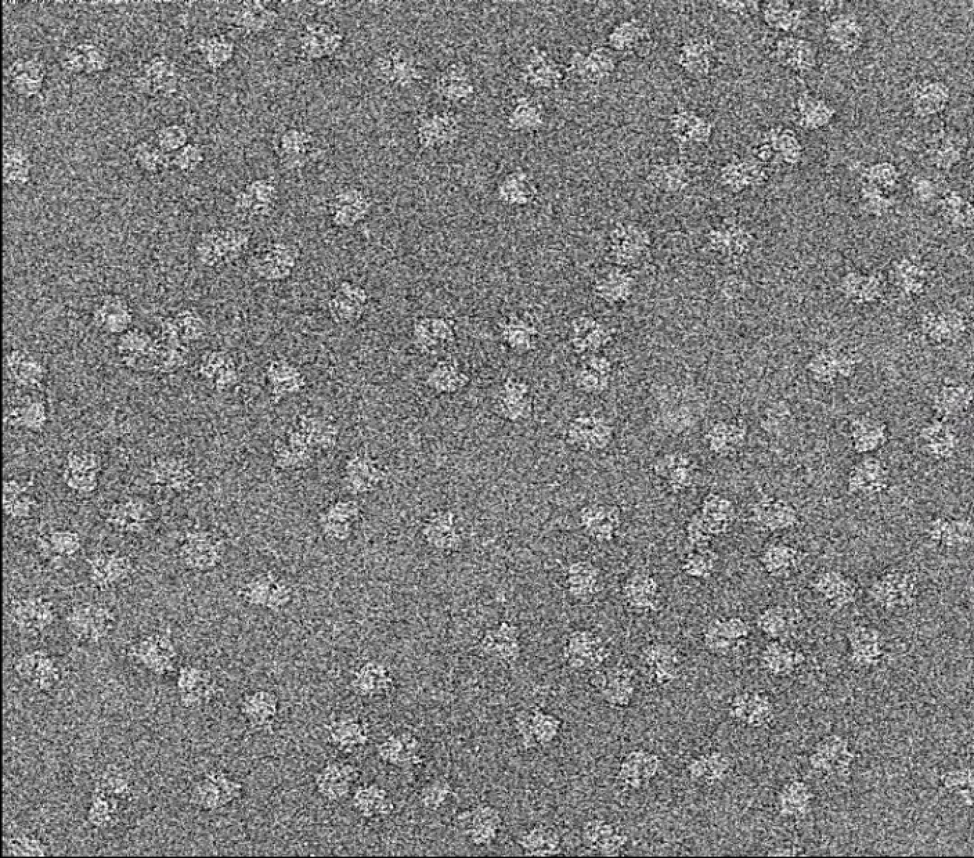
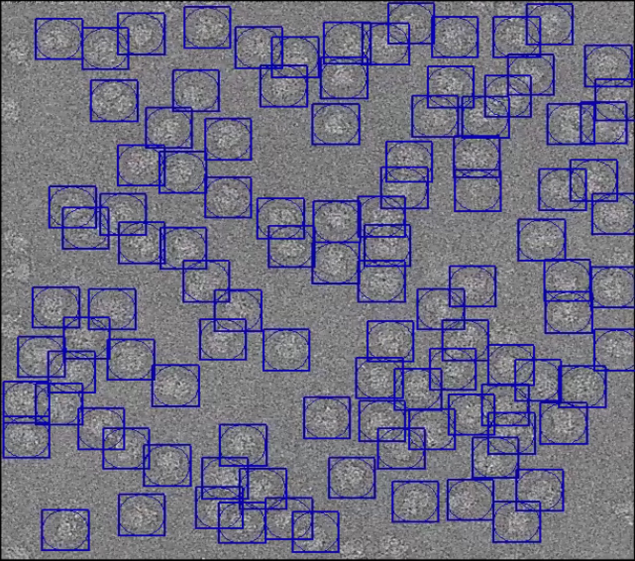
A particular application of great scientific importance that motivates this work is the particle detection task in single-particle cryo-electron microscopy (cryo-EM), which is currently the leading method for resolving the three-dimensional structure of molecules [25, 14]. In this method, a sample containing multiple copies of a molecule is rapidly frozen in a thin layer of ice, whereby the locations and orientations of the frozen molecules in the ice layer are unknown. An electron beam is transmitted through the frozen sample, resulting in a large, highly noisy, two-dimensional image containing two-dimensional smaller images of the molecules (technically, their tomographic projections) at unknown locations within the larger image. These two-dimensional small images are typically referred to as particles. An example cryo-EM image together with manually annotated particles is shown in Figure 1. One of the first steps towards resolving the three-dimensional structure of the molecule is locating the particles in the image, a step called “particle picking.” Currently, all particle picking algorithms, e.g., [39, 30, 12, 16] suffer from a high percentage of false positives (detecting “non-particles” as particles), thus requiring a time-consuming process of cleaning the data. The algorithm derived in this paper will allow to collect electron microscopy data sets with a low percentage of non-particle images, and will significantly speed up the processing of cryo-electron microscopy data. Moreover, it will eliminate the necessary manual intervention in current processing pipelines, which may introduce subjective bias into the analysis [21, 4]. We will demonstrate in Section 3 the applicability of our algorithm to simulated and experimental cryo-EM data sets, and present improvement compared to one of the existing standard software. Based on our theoretical derivations (Section 2.3) and empirical insights (Section 3), we discuss in Section 4 the limitations and possible extensions of our algorithm.
To summarize, the contribution of our paper is five-fold. First, we introduce a general and flexible observation model for object detection tasks. Second, we devise an object detection algorithm accompanied by performance guarantees for its power and error rate. In particular, we suggest a test statistic which is applicable to non-Gaussian data. Third, we introduce the notion of localization, which quantifies how accurately can we detect the centers of the objects. Fourth, we develop new proof techniques, which are essential in order to prove that the power of our algorithm approaches while controlling the error rate. Finally, we apply our algorithm to experimental cryo-EM data sets, demonstrating improvement compared to existing algorithms.
The data analysis and all simulations were implemented in Matlab. The code is available at https://github.com/ShkolniskyLab/object_detection_LSM/.
2 Theory
2.1 Problem setup
In this section, we introduce the observation model and define the object detection problem. We assume that the observable is given by
| (1) |
where consists of the objects to be detected and is a centered Gaussian stationary ergodic process on , representing the noise in the data. We assume that is observed on , where
| (2) |
is the closed hyper cube centered at with side length . If the hyper cube in (2) is open, we denote it by . Additionally, suppose that is given by
| (3) |
where is the (unknown) number of objects, , are known functions, compactly supported on , and orthonormal in , while the coefficients are unknown and depend on . Note that each in (3) is a deterministic function which is compactly supported within an open hypercube of a known side length , centered at an unknown location . We term this model the linear subspace model. Our goal is to estimate the objects’ centers given , , and .
Note that the proposed model is significantly more general than the model of [29, 9], as the objects are not required to be unimodal nor positive, and we only assume that the objects are spanned by some known basis functions, such as the Fourier basis, orthogonal polynomials, PCA basis, etc. Moreover, in contrast to [29, 9], we aim to estimate the unknown centers , and not just detect some arbitrary point within the support of each object.
2.2 Algorithm’s outline
A typical object detection algorithm consists of two main steps: a) applying a score map (or a heat map) on the observed data, which is a function that assigns a number to each position in the data; b) declaring all peaks in the score map larger than some threshold as the centers of the detected objects. We consider each value of the score map as a proxy for the presence of an object at that location. Two fundamental questions are how to design the score map and how to set the threshold so that the detection algorithm has high power and controlled FWER or FDR.
We first introduce the algorithm step by step, and then discuss its different components.
-
1.
Compute the score map
(4) where and is a linear convolution over .
-
2.
Select candidate peaks. We choose the highest peak in to be our first candidate for an object’s location. We then erase a box of size around this peak (the value of the parameter will be defined below). Then, we select the highest peak in the remaining data, and repeat this process until the remaining data is empty. Formally, we define a sequence of points
where is the number of steps until we cover . We denote the set of candidate peaks by .
-
3.
For with observed height , compute the test values . The test value for identifying peaks is
(5) where is the number of basis functions.
- 4.
The intuition behind step 1 above is as follows. The expression (4) is the energy of the projection of the observed data onto the set that spans the unknown objects. Since the noise is not spanned by this set of functions, we expect that projecting regions in the data containing objects would result in larger compared to areas that do not. We quantify this intuition in A.2. In light of step 1, in step , higher values of the score map are expected to indicate the presence of an object. We thus choose the highest peak in as the first candidate for an object location (and prove in A.8 that it indeed corresponds to an object with high probability). Since all pixels around this peak belong to that object, we remove them from subsequent peak searches, and repeat this process. The test value in step 3 allows to compute a detection threshold which distinguishes signal from noise by quantifying the expected peak height due to noise only. This is done in step 4 using a multiple hypothesis testing procedure. We show in Section 2.3 that the above procedure detects all objects, while controlling the error rate (under asymptotic conditions described in Section 2.3). The algorithm is illustrated in Figure 2.
2.3 Theoretical guarantees
To quantify the performance of the algorithm, we first need to rigorously define its power and error rate. As we would like to estimate the object centers from (3), we consider as a true positive (successful detection) a peak returned by our algorithm which is within distance from , for some chosen parameter . We would obviously like to be small, and discuss its choice below. We define to be the union of the neighborhoods about the centers (the true positive region), and the null region Having applied the algorithm of Section 2.2, the number of truly detected peaks and falsely detected peaks are
where is defined in (6). Both and are defined to be zero if is empty.
The FWER is defined as the probability of obtaining at least one falsely detected peak, formally given by
| (7) |
The false discovery rate (FDR) is defined as the expected proportion of falsely detected peaks,
| (8) |
where the expectation is taken with respect to the noise. The power of the algorithm corresponds to the ratio of objects detected by the algorithm. Formally, for a given threshold , we define
| (9) |
The indicator operator in (9) ensures that if more than one peak falls within the same neighborhood of some center, only one is counted, so that the power is not artificially inflated. The power is always non negative and less than : power equal means that we did not detect any objects, while power equal means that we detected all objects.
The parameter that appears in the above definitions cannot be made arbitrarily small. A necessary condition for the algorithm to find the objects is that it detects the objects when no noise is present. This implies that each peak detected in step 2 of the algorithm should be “close” to some . The condition ensuring this is given in the following definition.
Definition 2.1 (Localization property).
We say that satisfies the localization property if, for every , there exists some representative such that for all
where is a positive constant, is the coefficients vector of , is defined in (3), and is the scoring map applied to the clean objects.
We show in Appendix D how to compute a value of which satisfies this property for a given set of functions . Once has been set, our goal is to compute an optimal detection threshold in step 4 of the algorithm that will control the error rate (FWER or FDR) below a pre-specified level , while ensuring that the power is as close as possible to . We make the following assumptions.
Assumptions.
Let satisfy the localization property (Definition 2.1). Consider the following assumptions
-
1.
-
2.
, where is the boundary of the hypercube.
-
3.
, where .
-
4.
Set , then .
Assumption ensures that the objects are sufficiently separated (as a function of ). Assumption means that there are no objects near the boundary, as we want to detect only whole objects. Assumption states that the number of objects increases with , while the density of the object occurrences over is fixed. Finally, assumption states that the norms of the objects are large enough to overcome the noise.
We begin by controlling the FWER. Here, we set the threshold to be the smallest such that , where (recall that is the parameter used in step 2 of the algorithm). Then, the following holds.
Theorem 2.2.
Suppose the assumptions above hold. Then, the algorithm of Section 2.2 with and the Bonferroni threshold satisfies
Proof.
See Appendix B. ∎
To control the FDR below level , we apply the Benjamini-Hochberg procedure [5] in step 4 of the algorithm as follows:
-
1.
Sort the set in a non-decreasing order.
-
2.
Find the largest index such that , where .
-
3.
Define the threshold to be the smallest number such that .
-
4.
Declare all points in as the detected objects’ centers.
Since is a random variable, the expectation in (8) and (9) is taken over all possible realizations of the random threshold . We then have the following theorem.
Theorem 2.3.
Suppose the assumptions above hold. Then, the algorithm of Section 2.2 with and the Benjamini-Hochberg threshold satisfies
Proof.
See Appendix C. ∎
We comment that the model (1) was formulated in the continuous domain ( is continuous), whereas in applications we inevitably work with discretized data (such as images given by a discrete array of pixels). Our analysis suggests that extending Theorem 2.2 to the discrete case (when is given on a discrete finite set) is straightforward. In Theorem 2.3, it is relatively straightforward to prove that the power tends to one, but seems less trivial to prove the control of the FDR, as the current proof requires the continuity of some intermediate functions.
3 Numerical results
3.1 Simulations
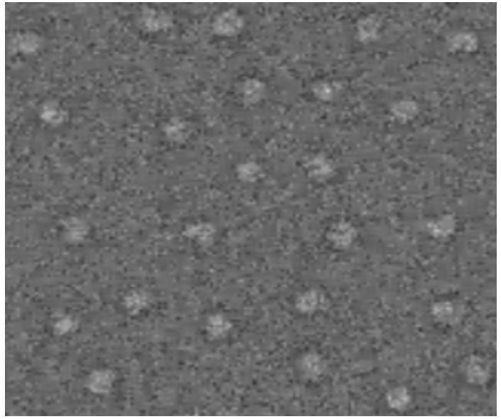
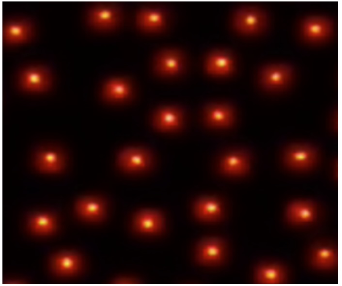
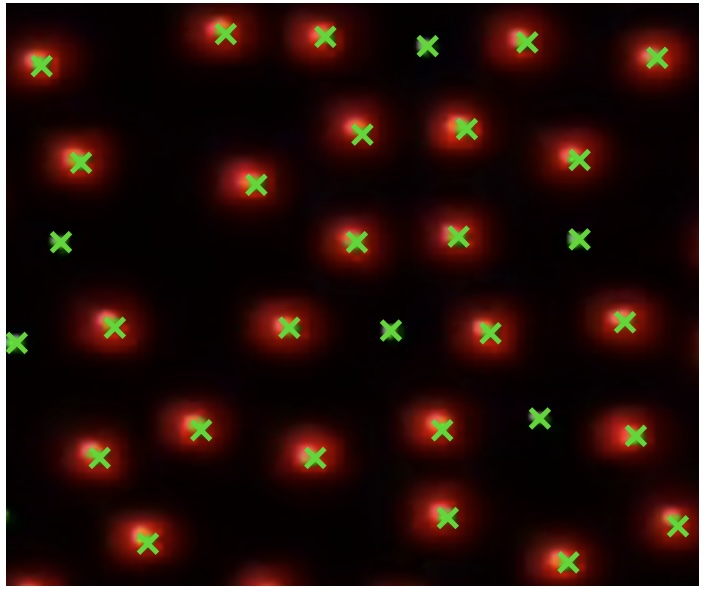
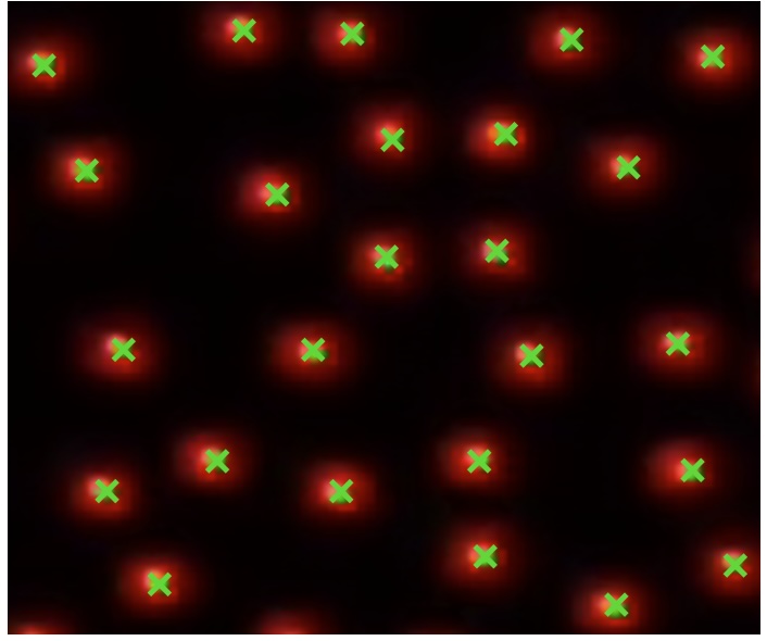
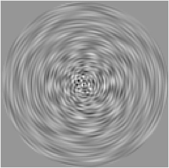
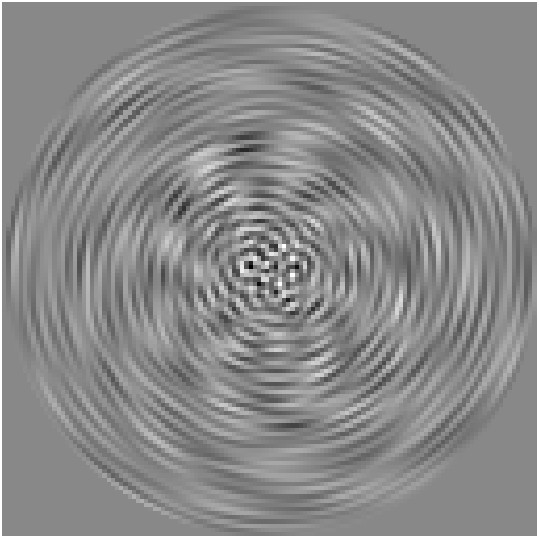
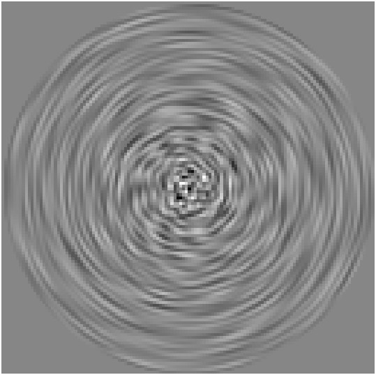
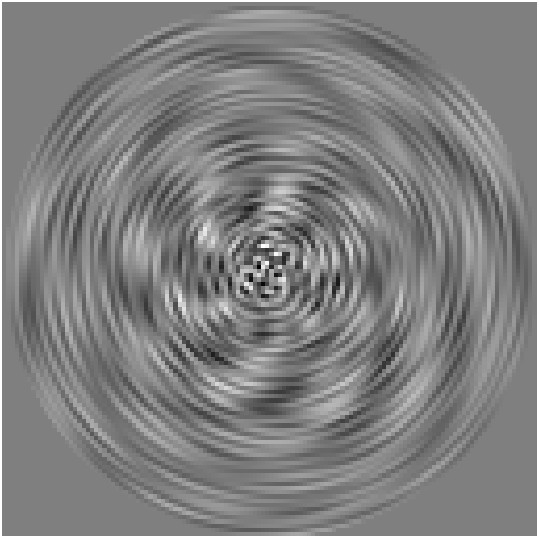
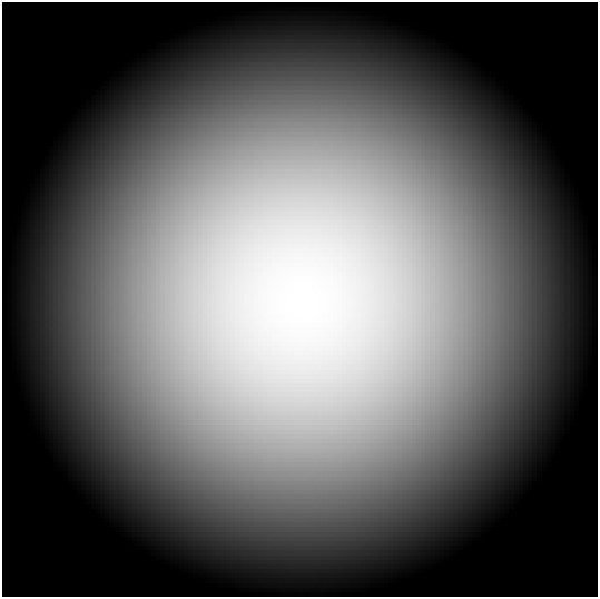
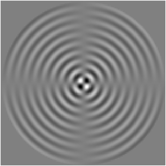
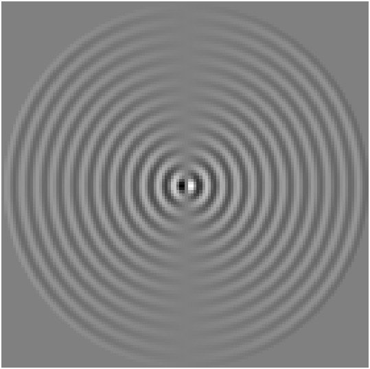
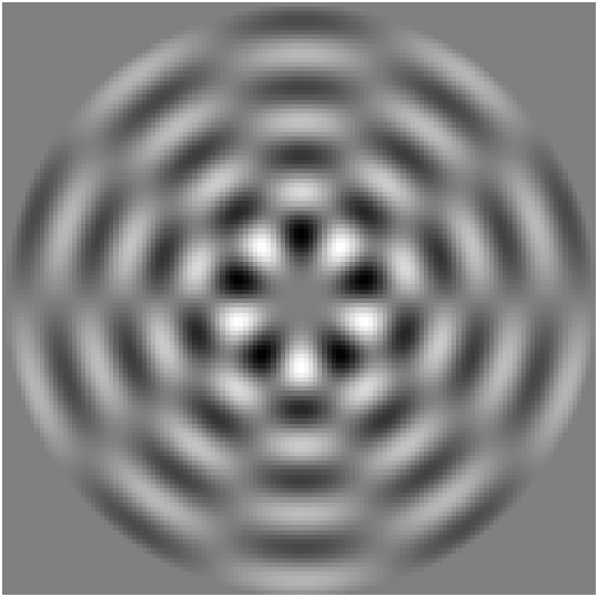
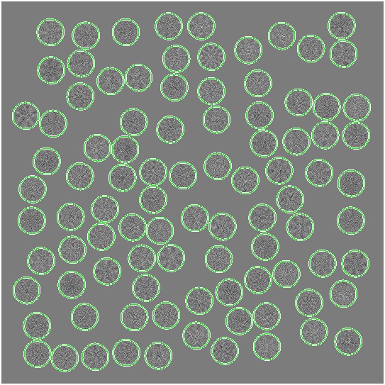
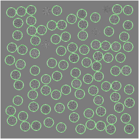
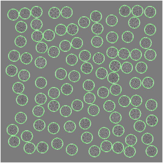
We first evaluate the performance of the proposed algorithm using simulations. In each experiment, we simulate a D realizations of of size pixels (i.e. ) which contain images (objects) of size pixels (). The objects are positioned at randomly chosen, non-overlapping locations, such that the density . Each object is formed as a linear combinations of Fourier Bessel functions [38], forcing symmetry so that the objects are real. The coefficients of each object are drawn independently from a uniform distribution over , such that the norm is . We use the method of Appendix D to conclude that pixels satisfies the localization property of Definition 2.1 and set . The noise (a realization of ) is a centered Gaussian process with covariance kernel , where . As a pre-processing step, we simulate only the pure noise in an image of size pixels, independently times. We denote each noise realization by . The image size of is chosen such that convolving it with the basis functions will give an output with the correct size needed to compute the samples defined in (5).
From the realization of , we compute the candidate set by applying steps and of the algorithm (see Section 2.2). By the law of large numbers, using , where , we estimate defined in (5) as , where and . Using the estimates of we apply step of the algorithm (see Section 2.2) with . Finally, we estimate the FWER, FDR, and the power by repeating the entire experiment described in this paragraph times independently, and using (7)–(9), where the expectation is estimated by the sample mean computed over the 500 trials. To quantify the noise level in the data, we define the signal-to-noise-ratio (SNR)
| (10) |
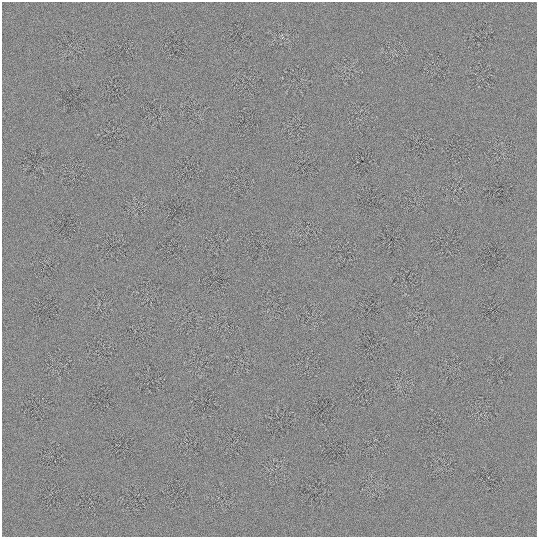
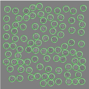
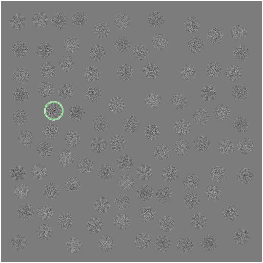
where and are defined in Assumption 4. Note that since each of the objects has norm equal to , we have that , and thus, determines the SNR. Figure 3 shows examples of both the objects and basis functions. Figure 4 shows examples of the detection results for both the Bonferroni and Benjamini-Hochberg procedures, described in Theorems 2.2 and 2.3. Table 1 presents the estimated FWER, FDR, and their power for different SNRs. As one can see, the error rates are always equal zero, indicating that the test value (5) is too conservative, which follows since it is given as times the maximum of . Instead, one can consider the more natural statistic , leading to an alternative test value
| (11) |
Unfortunately, proving performance guarantees when using the test value (11) by our current proof strategy requires the continuity of (11) with respect to , which we have not been able to establish. Yet, we demonstrate numerically the performance of the test value in (11). Table 2 presents the estimated FWER, FDR, and their power, for SNRs in which the test value defined in (5) fails. Note that the error rates are not zero as in Table 1 but still controlled.
| SNR | FWER | power | FDR | power |
|---|---|---|---|---|
Y Bonferroni Benjamini-Hochberg
SNR = 1
SNR = 0.5

SNR = 0.4

SNR = 0.35

| SNR | FWER | power | FDR | power |
|---|---|---|---|---|
3.2 Example of an experimental cryo-EM dataset
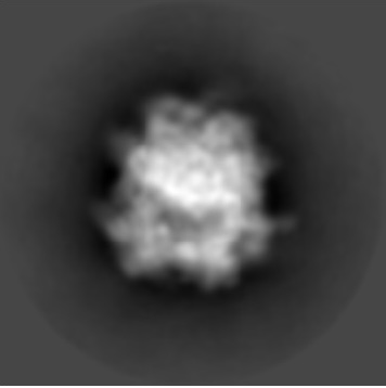
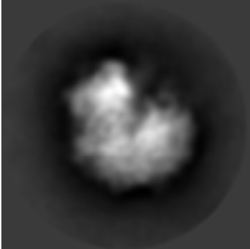
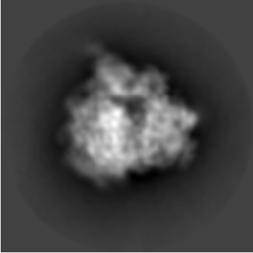
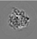
We next demonstrate our algorithm for template-based object detection in experimental data. In this setting, we are searching given templates in a large noisy image. The data consists of cryo-EM images of size pixels, taken from the Plasmodium Falciparum 80S ribosome (PF8r) data-set [34], downloaded from the Electron Microscopy Public Image Archive [23]. The size of the objects is approximately pixels and there are between to objects in each image. Due to memory constraints, we down-sample the images such that the size of the objects after downsampling is pixels (). To generate templates, we used the algorithm of [40], resulting in different two-dimensional views of the underlying molecule. Four views are shown in Figure 5. The basis used by our algorithm is generated by applying the Gram-Schmidt orthogonalization to the views. Four of the basis functions are shown in Figure 5. For the resulting basis, we set pixels, and used the method of Appendix D to numerically verify that this satisfies the localization property of Definition 2.1. We also set . Next, we need to generate noise samples following the distribution of the noise in the data. To that end, we identified noise patches in the data, estimated their (isotropic) covariance matrix, and generated Gaussian samples with mean zero and the estimated covariance. All subsequent steps of the algorithm are implemented as in Section 3.1 with the test value (11).
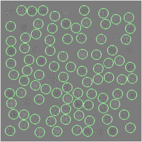
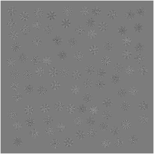
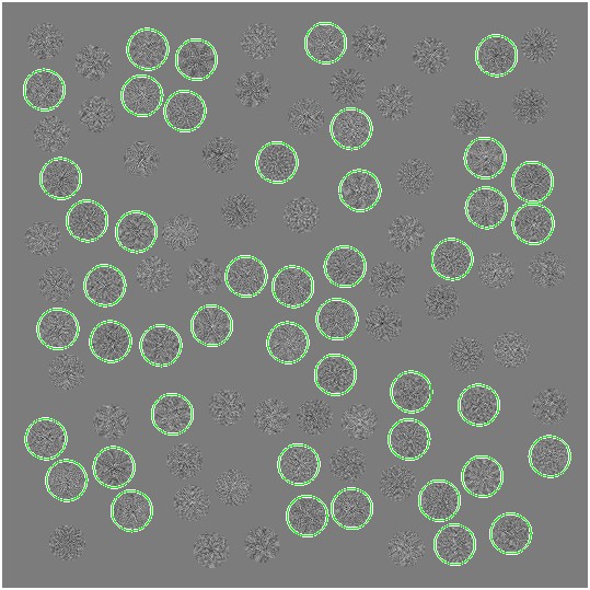
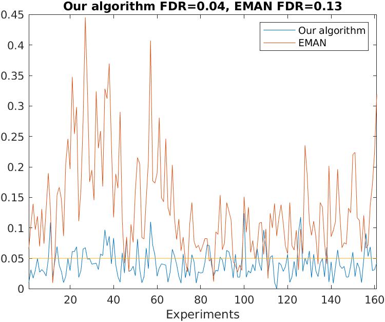
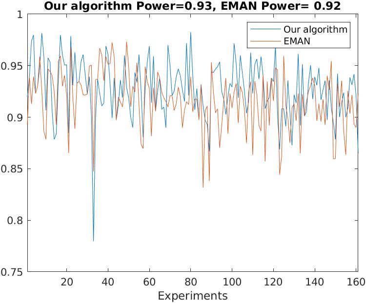
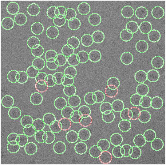
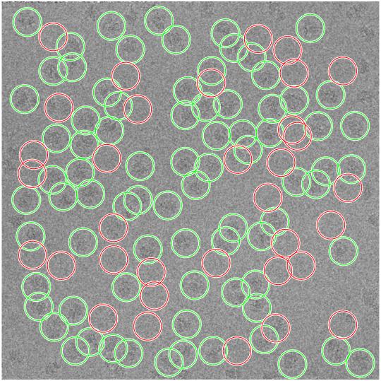
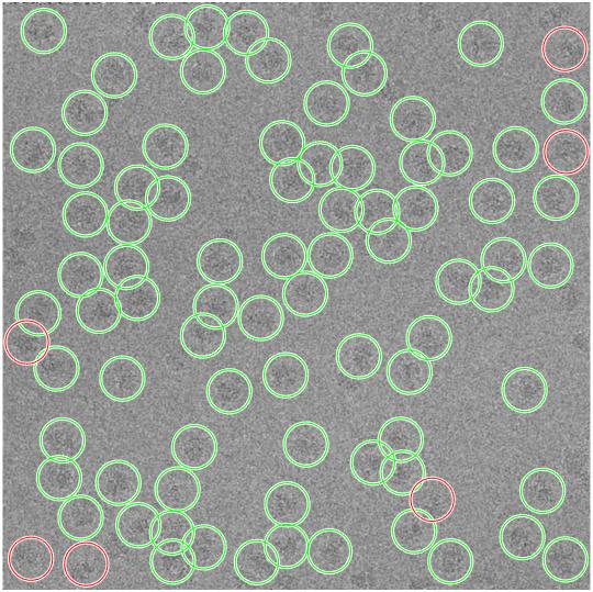
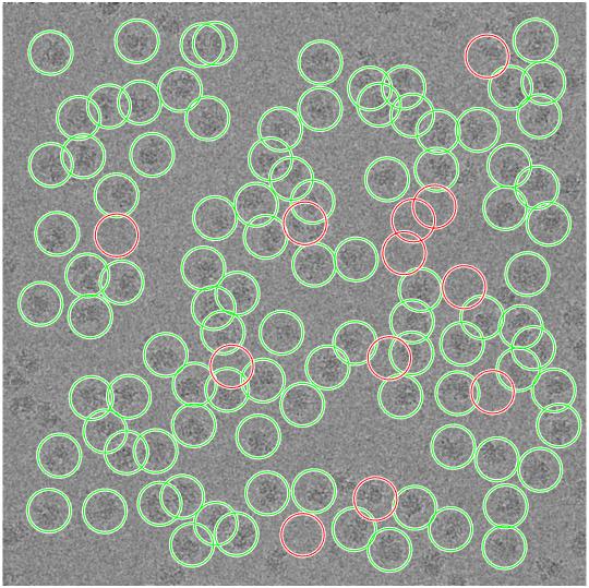
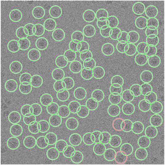
We compare the results of our algorithm with the results of the particle picking algorithm in EMAN [31] (one of the popular software packages for cryo-EM data processing). We use the same input to both algorithms. The detection threshold of the algorithm in EMAN is computed automatically by the software. To evaluate the results of both algorithms we used the benchmark dataset [13], which reports the centers of the objects in the data. Since the centers’ identification process in [13] is manual, it is subject to small errors. Therefore, we define true positive whenever an algorithm detects a point in the data that is up to pixels from the center reported in the benchmark dataset (this value corresponds to 50% of the radius of the object). Figure 6 presents the FDR and power for both algorithms. As one can see, the FDR of our algorithm is controlled, lower than EMAN’s and our power is higher. We do not present results for the FWER, as both algorithms make more than one mistake on each image (experiment), which leads to an FWER of . Finally, Figure 7 shows examples of the detection results. Note that our algorithm has higher number of true positives (green circles) than EMAN, while having fewer false positives (red circles).


EMAN Our algorithm
93

94
95
4 Discussion and future research
In this work, we presented an object detection algorithm that allows to control the power and error rates simultaneously. The performance bounds of the algorithm are proven in an asymptotic regime, though the numerical experiments show that it performs well in real-world scenarios, and in particular, in the non-asymptotic regime.
An important future work is deriving non-asymptotic performance bounds. In particular, we conjecture that we can replace the requirement that the norms of the objects tend to infinity by requiring that the projected SNR (see A.2) is sufficiently large. In addition, as noted in Section 3.1, the test value we use seems to be sub-optimal; we intend to analyze the performance of the proposed algorithm with the alternative test value (11). The main difficulty is proving that this test value is continuous with respect to . Finally, we wish to design bases that allow to be as small as possible.
Acknowledgments
Amitay Eldar was supported by NSF-BSF award 2019733. Keren Mor Waknin was supported in part by a fellowship from the Edmond J. Safra Center for Bioinformatics at Tel-Aviv University and The Jacob and Riva Damm Endowment Fund. Tamir Bendory supported in part by BSF grant no. 2020159, NSF-BSF grant no. 2019752, and ISF grant no.1924/21. Samuel Davenport and Armin Schwartzman were supported in part by NIH/NIBIB Award R01EB026859. Yoel Shkolnisky was supported in part by NIH/NIGMS Award R01GM136780-01.
Appendix A Auxiliary claims
Claim A.1.
Let and , then, .
Proof.
Denote , then,
where the fifth equality is due to change of variables and the seventh equality follows from Assumption 1. ∎
Claim A.2 (Projected SNR is higher at an object’s center).
Let . Denote by the input signal-to-noise ratio and by the projected signal-to-noise ratio, where . Then, for some .
Proof.
We can write where is an orthonormal complement of and are random variables. Denote . Then,
where the second equality follows from Parseval’s theorem, and the third follows from the monotone convergence theorem. On the other hand, by stationarity, for each ,
where . The latter, combined with A.1, implies that
∎
Claim A.3.
, where , , .
Proof.
∎
Claim A.4 (Controlling the growth of the mixed term ).
Let , and denote by the set of indices of centers such that . Then,
where , and is a positive constant.
Proof.
Let , then, as in A.1, by a change of variable we get
Hence,
By the Cauchy–Schwartz inequality,
Applying the Cauchy–Schwartz inequality again, and using the fact that , for all , we get that
Note that for any , since the centers are at least at distance from each other, there can be at most centers satisfying , so . Hence,
∎
Definition A.5.
Let . We say if there exist positive constants and that do not depend on , such that .
Claim A.6 (Controlling the growth of the projected noise).
Proof.
Denote for all , . The first inequality follows immediately by
| (12) |
surely for all . Then,
where the last inequality is the union bound. Let us bound the probability
To this end, divide into boxes of volume 1. Then,
Now, set
By the Borell–TIS inequality [1] we get,
so that
where , , and . Overall, we get
∎
Claim A.7.
The test value defined in (5) i.e. is continuous for all .
Proof.
By [37], for each , is a continuous random variable. For all ,
which implies the continuity of each of the . Then,
which yields the continuity of as the maxima of continuous random variables.
∎
Claim A.8 (All objects are picked first).
Let the assumptions from Assumptions hold, and suppose that our algorithm is applied with . Denote by the event that the first points in are in . Then
| (13) |
where is defined in A.5.
Proof.
Recall that , and denote . Note that . We will prove that for all ,
This will complete the proof as
where the limit tends to zero by Assumptions 3 and 4. Assume (without loss of generality) that . We start with . Recall that is the representative defined in Definition 2.1, and that . Note that
Now, using A.4, we get that
Altogether we get,
The latter yields,
where we used the localization property (Definition 2.1), since . This implies
Using A.6, we get that for all ,
which yields,
For , we are going to intersect it with the event which means we want to bound the probability that and . Note that for a unique . Denote . Since then, on the event , we have that , which implies
Now, in order to bound and with , first observe that . Indeed, since and for all , it holds that . Second, for , note that since and , then, , which implies that . Hence . Combining the latter with A.4, we get
In order to bound we split to cases. If , then, and , so it follows from Definition 2.1 that
Otherwise, , which means that and , which implies that , and hence, we can apply Definition 2.1 again to get
To conclude, in both cases we have , and thus,
Overall, we get
Then, we can repeat this argument for all and induction to get
∎
Claim A.9 (The multiple testing procedure stops after more than or equal to steps).
Let the assumptions from Assumptions hold, and suppose that our algorithm is applied with . Denote by , the events that the Bonferroni or Benjamini-Hochberg procedures, defined in Theorems 2.2 and 2.3, stop after more than or equal to steps. Then,
| (14) |
where is defined in A.5.
Proof.
We start with the Benjamini-Hochberg procedure. Recall that is the largest index such that
Let . Recall that is the event that the first points in are in . In A.8 we proved that . Set , where defined in 2.1. By A.6, and the union bound it holds that . Combining both we have that
where the limit is zero due to Assumptions 3 and 4. We shall prove that such that for all ,
which finishes the proof. Assume without loss of generality that . Let . Then, (see definition of in Section 2.2). Now,
where the third equality follows from A.3, the forth inequality is due to non-negativity of and the fifth inequality follows by A.4 and Definition 2.1. The six equality is due to the fact that , the seven inequality follows from the definition of . In the last two inequalities, we used A.6 and Assumptions (3),(4). To conclude we proved that for every and , the BH procedure stops after more than or equal to steps which means by definition that .
For the Bonferroni procedure, we use the last inequality to get
which implies that such that it holds that . ∎
Recall that for all , where and are defined in Sections 2.2 and 2.3. Define for all
| (15) |
where , , and is a partition of into evenly sized closed hypercubes of side length (assuming without loss of generality that is divided by ).
Claim A.10.
Let the assumptions from section (Assumptions) hold, and suppose that our algorithm is applied with . On the event (defined in Claim A.8) where the first points in are in , it holds that
for all .
Proof.
Note that . The algorithm in Section 2.2 gives that if , then , and therefore, there is only one point from that can be in . The latter yields that and thus
On the event , we have that , then, again by the algorithm in Section 2.2, for all : . Hence, on the event ,
∎
Appendix B FWER control and power consistency
Proof of Theorem 2.2.
We start with the power. Since our algorithm erases cubes of side length (step in Section 2.2) and (because , see Appendix D), there is at most one element from in each -neighborhood of the centers. Then for all ,
We shall prove that
On the event , it holds that . By Claims A.8 and A.9,
Hence, we get
Recall that for all , and that the test function 5 is defined by . Note that due to stationarity of we have that
Next we show that the FWER is controlled i.e.
Now, applying Markov’s inequality and using Claim A.10 and the trivial bound , we have that,
where the fifth inequality follows from A.8.. Taking concludes the proof by Assumptions 3 and 4. ∎
Appendix C FDR control and power consistency
Proof of Theorem 2.3.
The proof of power consistency is the same as in Appendix B. For the FDR, we shall use subsequences of , so we denote , , , and . We need to prove that
Without the loss of generality, assume . Set to be the event where the first points in are in , and that the BH algorithm (defined in Section 2.3) stops after more than steps i.e. . By Claims A.8, A.9 and Assumption 3 in Section 2.3, there exists such that for all ,
| (16) |
Now, consider the event
and note that
Throughout the proof, we will rely on the ergodicity of the process (defined in (1)) which implies that for all ,
| (17) |
Set
| (18) |
where and is our probability space for the process . Then, by (17), for all , , which implies . Set and note that . We have,
Now, for all
Hence
where the last inequality follows from Jensen’s inequality. By claim A.10, we have that for all , on the event , . By monotonicity of the map ,
The latter expression is connected to the test value (5) as for a deterministic threshold , . Though is random, the next lemma overcomes the randomness by bounding it from below with a random sequence that converges to a deterministic threshold.
Lemma C.1.
Let be the smallest solution of . Then, there exists a random sequence such that for all and
-
•
-
•
.
The Proof of Lemma C.1 is in Section C.2.
∎
This lemma, combined with the monotonicity of , implies that
By Egorov’s Theorem [24], there exists such that and
which yields that there exists such that for all and
It follows that
where in we trivially bound . To conclude, for all
Hence,
where is a positive constant. Taking , by continuity of (see A.7), we get
∎
C.2 Proof of Lemma C.1
First, we will prove that on , every convergent subsequence of converge to a solution of the inequality . Recall that on , The first points in the candidate set are in , and the Benyamini-Hochberg procedure (defined in section 2.3) stops after more then steps. As a result, the number of detected objects, denoted by , equal to the number of objects plus the number of false positives. The latter, combined with the definition of the BH-threshold (see Section 2.3), gives for all ,
Let , and note that is bounded. Indeed, by (16) for all , and so,
| (19) |
Moreover, by definition, and hence
| (20) |
Since is monotone decreasing, is bounded. Consider , a convergent subsequence of . Then, for every there exists a large enough such that for every ,
Let , and choose such that . By A.10 and the monotonicity of , we get for all ,
| (21) | ||||
Since (defined in (18)), taking the limit in (21) and using the continuity of yields
Using again the monotonicity of , we get that
Taking limit over in the last inequality implies that satisfies
hence
Set , where is the smallest solution for and let . We want to prove that . Let . Since is bounded, there exists a convergent subsequence where . Now,
which implies . We proved that every convergent subsequence of converges to the same deterministic , and therefore .
To conclude, we found a random sequence such that for all and , and as desired.
Appendix D Estimating which satisfies Definition 2.1
Recall Definition 2.1: we say that satisfies the localization property if for all , there exists some representative such that
where , and is a positive constant. Clearly, such depends on the given , the unknown coefficients and locations of the objects, all are defined in Section 2.1. Nonetheless, in all cases, satisfies Definition 2.1, hence such s always exists. Indeed, for , it holds that for all , and by A.1, it holds that for all . Therefore, taking suffices. Our goal is to find satisfying Definition 2.1 which is smaller than . To that end, we will develop an inequality whose solutions satisfy Definition 2.1, see D.4, and use it throughout Section 3 in order to validate that a given value of can be used.
First we note that can be written as a bi-linear form involving the inner product of the translated basis functions. Set the matrix to be, for all ,
is a real symmetric matrix, which depends on .
Claim D.1.
| (22) |
Proof.
Denote . Then,
∎
Denote by
where are the minimal and maximal eigenvalue respectively.
Claim D.2.
Let , and assume for all . Denote . Then,
-
1.
,
-
2.
.
Proof.
For the first part, let , then
| (23) | ||||
The second equality in the latter expression is due to the fact that if and the centers are more than apart, then all the other terms in the sum of are zero. The last inequality in the latter expression is a known bound in linear algebra [22].
For the second part, let . Then,
| (24) | ||||
where the last inequality is again a known bound from linear algebra [22]. ∎
By D.2, we have and ,
As mentioned above, is a function of , which makes translation invariant with respect to the object centers and . That is, for all we have , which implies the same for the eigenvalues of . In particular, for ,
and for
To conclude,
where is defined on D.2. Now, taking the supremum with respect to and all possible locations of objects yields the following definition.
Definition D.3.
for
Claim D.4.
Assume that . Then, given such that , implies that satisfies Definition 2.1.
Proof.
Choose such that . By Definition D.3, for which . Using the shift invariant property of and Definition D.3:
| (25) |
Assume without loss of generality that . Then, by D.2
Next, if , then , which implies where defined in D.2. By D.2, the shift invariant property of , and Definition D.3, such that ,
We can repeat this argument for , and get the desired property, which completes the proof. ∎
Recall that our algorithm requires as input a that satisfies Definition 2.1 (to ensure the statistical guarantees outlined in Theorems 2.2 and 2.3). When processing numerical data, as discussed in Section 3, the basis functions spanning the objects are represented on a grid that scales with the size of the objects (denoted by ). Following the assertion made in D.4, we seek to determine such a value for , by numerically solving the inequality . To that end, we iterate over , starting with the smallest possible value which is computationally feasible, for example, the minimum distance between two points on the grid. In each iteration, in order to estimate , we computes for all possible centers and points on the grid. This iterative process persists until invariably concluding at since (as explained earlier in this section).
References
- [1] Robert J Adler and Jonathan E Taylor. Random fields and geometry, chapter 2. Springer Science & Business Media, 2007.
- [2] Dror Aiger and Hugues Talbot. The phase only transform for unsupervised surface defect detection. In 2010 IEEE Computer Society Conference on Computer Vision and Pattern Recognition, pages 295–302. IEEE, 2010.
- [3] Jinwon An and Sungzoon Cho. Variational autoencoder based anomaly detection using reconstruction probability. Special lecture on IE, 2(1):1–18, 2015.
- [4] Tamir Bendory, Alberto Bartesaghi, and Amit Singer. Single-particle cryo-electron microscopy: Mathematical theory, computational challenges, and opportunities. IEEE signal processing magazine, 37(2):58–76, 2020.
- [5] Yoav Benjamini and Yosef Hochberg. Controlling the false discovery rate: a practical and powerful approach to multiple testing. Journal of the Royal statistical society: series B (Methodological), 57(1):289–300, 1995.
- [6] T. Bepler, A. Morin, M. Rapp, J. Brasch, L. Shapiro, A. J. Noble, and B. Berger. Positive-unlabeled convolutional neural networks for particle picking in cryo-electron micrographs. Nature Methods, 16(11):1153–1160, 2019.
- [7] Giacomo Boracchi, Diego Carrera, and Brendt Wohlberg. Novelty detection in images by sparse representations. In 2014 IEEE Symposium on Intelligent Embedded Systems (IES), pages 47–54. IEEE, 2014.
- [8] P. Brutti, C. R. Genovese, C. J. Miller, R. C. Nichol, and L. H. Wasserman. Spike hunting in galaxy spectra. Technical report, Carnegie Mellon University, 2005.
- [9] D. Cheng and A. Schwartzman. Multiple testing of local maxima for detection of peaks in random fields. The Annals of Statistics, 45(2):529–556, 2017.
- [10] Samuel Davenport, Thomas E Nichols, and Armin Schwarzman. Confidence regions for the location of peaks of a smooth random field. arXiv preprint arXiv:2208.00251, 2022.
- [11] Axel Davy, Thibaud Ehret, Jean-Michel Morel, and Mauricio Delbracio. Reducing anomaly detection in images to detection in noise. In 2018 25th IEEE International Conference on Image Processing (ICIP), pages 1058–1062. IEEE, 2018.
- [12] J. M. de la Rosa-Trevín, J. Otón, R. Marabini, A. Zaldívar, J. Vargas, J. M. Carazo, and C. O. S Sorzano. Xmipp 3.0: an improved software suite for image processing in electron microscopy. Journal of structural biology, 184(2):321–328, 2013.
- [13] Ashwin Dhakal, Rajan Gyawali, Liguo Wang, and Jianlin Cheng. A large expert-curated cryo-EM image dataset for machine learning protein particle picking. Scientific Data, 10(1):392, 2023.
- [14] Editorial. Method of the year 2015. Nature Methods, 13(1):1, January 2016.
- [15] Thibaud Ehret, Axel Davy, Jean-Michel Morel, and Mauricio Delbracio. Image anomalies: A review and synthesis of detection methods. Journal of Mathematical Imaging and Vision, 61:710–743, 2019.
- [16] A. Eldar, I. Amos, and Y. Shkolnisky. ASOCEM: Automatic segmentation of contaminations in cryo-EM. Journal of Structural Biology, 214(3):107871, 2022.
- [17] Amitay Eldar, Boris Landa, and Yoel Shkolnisky. KLT picker: Particle picking using data-driven optimal templates. Journal of structural biology, 210(2):107473, 2020.
- [18] C. Geisler, A. Schönle, C. von Middendorff, H. Bock, C. Eggeling, A. Egner, and S. W. Hell. Resolution of in fluorescence microscopy using fast single molecule photo-switching. Applied Physics A, 88:223––226, 2007.
- [19] C. R. Genovese, N. A. Lazar, and T. Nichols. Thresholding of statistical maps in functional neuroimaging using the false discovery rate. NeuroImage, 15(4):870–878, 2002.
- [20] Bénédicte Grosjean and Lionel Moisan. A-contrario detectability of spots in textured backgrounds. Journal of Mathematical Imaging and Vision, 33:313–337, 2009.
- [21] Richard Henderson. Avoiding the pitfalls of single particle cryo-electron microscopy: Einstein from noise. Proceedings of the National Academy of Sciences, 110(45):18037–18041, 2013.
- [22] Kenneth Hoffman. Linear algebra, chapter 10. Pearson, 1971.
- [23] Andrii Iudin, Paul K Korir, Sriram Somasundharam, Simone Weyand, Cesare Cattavitello, Neli Fonseca, Osman Salih, Gerard J Kleywegt, and Ardan Patwardhan. Empiar: the electron microscopy public image archive. Nucleic Acids Research, 51(D1):D1503–D1511, 2023.
- [24] Vasilevich Kolmogorov, Nikolaevich. Introductory real analysis, chapter 8. Courier Corporation, 1975.
- [25] D. Lyumkis. Challenges and opportunities in cryo-EM single-particle analysis. The Journal of biological chemistry, 294(13):5181–5197, 2019.
- [26] Ariane Marandon, Lihua Lei, David Mary, and Etienne Roquain. Machine learning meets false discovery rate. arXiv preprint arXiv:2208.06685, 2022.
- [27] Der-Baau Perng, Ssu-Han Chen, and Yuan-Shuo Chang. A novel internal thread defect auto-inspection system. The International Journal of Advanced Manufacturing Technology, 47:731–743, 2010.
- [28] G Rupert Jr et al. Simultaneous statistical inference. Springer Science & Business Media, 2012.
- [29] A. Schwartzman, Y. Gavrilov, and R. J. Adler. Multiple testing of local maxima for detection of peaks in 1D. The Annals of Statistics, 39(6):3290–3319, 2011.
- [30] G. Tang, L. Peng, P. R. Baldwin, D. S. Mann, W. Jiang, I. Rees, and S. J. Ludtke. EMAN2: an extensible image processing suite for electron microscopy. Journal of Structural Biology, 157(1):38–46, 2007.
- [31] Guang Tang, Liwei Peng, Philip R. Baldwin, Deepinder S. Mann, Wen Jiang, Ian Rees, and Steven J. Ludtke. Eman2: An extensible image processing suite for electron microscopy. Journal of Structural Biology, 157(1):38–46, 2007. Software tools for macromolecular microscopy.
- [32] J. E. Taylor and K. J. Worsley. Detecting sparse signals in random fields, with an application to brain mapping. Journal of the American Statistical Association, 102(479):913–928, 2007.
- [33] D-M Tsai and C-Y Hsieh. Automated surface inspection for directional textures. Image and Vision computing, 18(1):49–62, 1999.
- [34] Wilson Wong, Xiao-chen Bai, Alan Brown, Israel S Fernandez, Eric Hanssen, Melanie Condron, Yan Hong Tan, Jake Baum, and Sjors HW Scheres. Cryo-EM structure of the Plasmodium falciparum 80s ribosome bound to the anti-protozoan drug emetine. eLife, 3:e03080, jun 2014.
- [35] K. J. Worsley, S. Marrett, P. Neelin, A. C. Vandal, and A. C. Friston, K. J.and Evans. A unified statistical approach for determining significant signals in images of cerebral activation. Human Brain Mapping, 4(1):58–73, 1996.
- [36] Xianghua Xie and Majid Mirmehdi. Texems: Texture exemplars for defect detection on random textured surfaces. IEEE transactions on pattern analysis and machine intelligence, 29(8):1454–1464, 2007.
- [37] Donald Ylvisaker. A note on the absence of tangencies in gaussian sample paths. The Annals of Mathematical Statistics, 39(1):261–262, 1968.
- [38] Zhizhen Zhao and Amit Singer. Fourier–Bessel rotational invariant eigenimages. JOSA A, 30(5):871–877, 2013.
- [39] J. Zivanov, T. Nakane, B. O. Forsberg, D. Kimanius, W. J. Hagen, E. Lindahl, and S. H. Scheres. New tools for automated high-resolution cryo-EM structure determination in RELION . Elife, 7:e42166, 2018.
- [40] Jasenko Zivanov, Takanori Nakane, Björn O Forsberg, Dari Kimanius, Wim JH Hagen, Erik Lindahl, and Sjors HW Scheres. New tools for automated high-resolution cryo-EM structure determination in relion. eLife, 7:e42166, nov 2018.
- [41] Maria Zontak and Israel Cohen. Defect detection in patterned wafers using multichannel scanning electron microscope. Signal processing, 89(8):1511–1520, 2009.
- [42] Maria Zontak and Israel Cohen. Defect detection in patterned wafers using anisotropic kernels. Machine Vision and Applications, 21:129–141, 2010.