.tifpdf.pdfconvert #1 .tif

Reevaluating coexistence and stability in ecosystem networks to address ecological transients: methods and implications

Sarah A. Vollert^a,b,∗, Christopher Drovandi^a,b, & Matthew P. Adams^a,b,c

^aCentre for Data Science, Queensland University of Technology, Brisbane, Australia

^bSchool of Mathematical Sciences, Queensland University of Technology, Brisbane, Australia

^cSchool of Chemical Engineering, The University of Queensland, St Lucia, Australia

^∗Corresponding author. E-mail: sarah.vollert@hdr.qut.edu.au

Abstract

Representing ecosystems at equilibrium has been foundational for building ecological theories, forecasting species populations and planning conservation actions. The equilibrium “balance of nature” ideal suggests that populations will eventually stabilise to a coexisting balance of species. However, a growing body of literature argues that the equilibrium ideal is inappropriate for ecosystems. Here, we develop and demonstrate a new framework for representing ecosystems without considering equilibrium dynamics. Instead, far more pragmatic ecosystem models are constructed by considering population trajectories, regardless of whether they exhibit equilibrium or transient (i.e. non-equilibrium) behaviour. This novel framework maximally utilises readily available, but often overlooked, knowledge from field observations and expert elicitation, rather than relying on theoretical ecosystem properties. We developed innovative Bayesian algorithms to generate ecosystem models in this new statistical framework, without excessive computational burden. Our results reveal that our pragmatic framework could have a dramatic impact on conservation decision-making and enhance the realism of ecosystem models and forecasts.

1 Introduction

The equilibrium perspective is ubiquitous in ecology. Much of our ecological theory¹; ²; ³; ⁴; ⁵; ⁶; ⁷; ⁸; ⁹; ¹⁰ and conservation decision making¹¹; ¹²; ¹³; ¹⁴; ¹⁵; ¹⁶; ¹⁷ has been achieved by representing ecosystems at equilibrium. This “balance of nature” ideal suggests that in the long term ecosystem populations will stabilise towards a balance of coexisting species¹⁸.

Simple equilibrium concepts have been highly useful for representing ecosystems generally ^{1; 2; 4; 7}, or in the absense of data ¹¹; ¹⁷; ¹³. Ecosystems are commonly represented as stably coexisting communities ⁴; ⁷; ⁹; ¹¹; ¹³, which can be thought of as two separate constraints: feasibility and stability. Ecosystem feasibility (a concept aligned with persistence and coexistence) suggests that steady-state populations must be positive, as a negative abundance would be meaningless ⁵; ⁸; ⁷. Stability is another commonly assumed feature of ecosystems, such that the system can recover from small changes to species abundances ³. Models constructed using constraints like these have been used in practice to analyse potential conservation actions ¹¹; ¹⁷; ¹⁴; ¹⁵; ¹²; ¹⁶ and to advance theoretical knowledge of ecosystem formation and function ¹; ¹⁰; ⁷; ⁴; ⁶.

However, feasible and stable equilibria cannot be directly observed in an ecosystem (since they are a product of the modelling), and are therefore a challenge to verify through empirical evidence ¹⁹; ²⁰. Here, along with with a growing body of literature, we question whether this idealistic representation of ecosystems is appropriate, particularly in the context of conservation ²¹; ¹⁸; ¹⁹; ²⁰; ²²; ²³; ²⁴; ²⁵.

Feasibility and stability describe ecosystem behaviour near equilibrium, such that population dynamics are not affected by strong abiotic or biotic factors ²⁶. In the modern world, where climate change, human development, and invasive species are persistent threats across the globe, ecosystems are rarely unaffected by strong external factors ²⁷; ²². This mismatch between modelled equilibrium states, and the disturbances seen in nature brings into question the use of equilibrium assumptions ²⁸; ²³; ²².

While ecosystems may appear to be exhibiting steady-state equilibrium behaviour, this could be a mismatch between human and ecological timescales ¹⁹. Not all ecosystems will always be in equilibrium, and they may instead be exhibiting long transient dynamics ²¹; ¹⁹; ²⁴; ²⁰, such that the ecosystem exhibits non-equilibrium slow-changing behaviour ²⁴. Representing ecosystems using equilibrium perspectives when compared to long transients yields qualitatively different model parameterisations ²⁹, and different model-informed conservation decision making ²⁵. Yet, it is a challenge to even identify if an ecosystem is experiencing long transient or equilibrium behaviour ²⁰; ³⁰.

Despite these criticisms, equilibrium perspectives remain pervasive in ecological modelling ²⁴; ²⁵. To our best knowledge, there is currently no method for constraining ecosystem model behaviour that does not rely on time series data or equilibrium assumptions. Since population monitoring data is often sparse, noisy or unavailable ³¹; ³²; ³³; ¹¹, the equilibrium perspective is therefore needed to represent ecosystems without investing significant time and money into data collection.

Here, we propose a novel framework to accommodate constraints far more pragmatic than stable and feasible equilibria. To illustrate the framework, we propose three new sets of constraints. Firstly, we introduce the option to restrict population sizes to within expert-elicited limits, such that models that yield unrealistic populations are excluded. Secondly, we relax the assumption forcing ecosystems to be represented at equilibrium, and instead consider an equilibrium-agnostic population trajectory-based alternative to address the likely common situation of transient (non-equilibrium) ecosystem dynamics ²⁹. Finally, we introduce the option to limit population fluctuations based on field knowledge, to restrict populations from growing or shrinking at unobserved or extreme rates.

To implement this new framework, we develop a novel approach to generating ensembles of parameter sets whose model predictions match a set of constraints. Approximate Bayesian algorithms ³⁴ provide a path for parameterising using non-data constraints, but new algorithms are needed to parameterise these models in an efficient manner. Here, we significantly extend an approximate Bayesian sequential Monte Carlo algorithm ¹³ to rapidly parameterise time-series trajectories where the previous approach is too computationally infeasible to consider.

Our new framework, together with statistical advances that make it practically accessible, can produce far more pragmatic representations of ecosystems, without needing to distinguish between equilibrium or transient (i.e. non-equilibrium) behaviour. To our best knowledge, this is the first equilibrium-agnostic framework for representing ecosystems without data. To do so, we maximally utilise expert knowledge and/or field observations – a readily available and often overlooked source of information. This new framework has the potential for dramatic impact on the management of complex ecosystems, improving both the precision of the models that represent these ecosystems and the confidence in any forecasted scenarios in these ecosystems.

2 Results

Starting from the classic equilibrium constraints – feasible and stable equilibria (set (1) in Table 1) – we demonstrated a series of increasingly pragmatic alternatives for representing ecosystems without data (see Table 1 for a summary; full details are provided in the Methods 4.1), either by constraining the long-term equilibrium behaviour (set (2)) or when considering finite population trajectories (sets (3) and (4)). We demonstrate these new pragmatic constraints for generalised Lotka Volterra models – a common choice in the literature ⁴; ¹¹; ³⁵ – combined with our efficient statistical framework for generating parameter sets that satisfy the constraints. Here, our results illustrate that elicited knowledge of expected populations (sets (2)-(4)), or unobserved population fluctuations (set (4)) can be used in place of equilibrium assumptions to yield knowledge-derived representations of ecosystems.

Set of constraints	Description	Mathematical constraint
(1) Positive and stable equilibria	The long term behaviour of the system will have coexistence of all species, and will be able to recover from small changes to populations. These constraints are commonly considered in the literature (e.g., Baker et al. 11; Allesina and Tang 1; Song et al. 8).	Equilibrium populations are positive, and stability is achieved when the real part of the eigenvalues of the Jacobian evaluated at the equilibrium are negative.
(2) Bounded and stable equilibria	The long term behaviour of the system will have bounded populations, and will be able to recover from small changes to populations. Here, equilibrium abundances are restricted to expert elicited “reasonable” limits.	Equilibrium populations are within specified bounds, and stability is achieved when the real part of the eigenvalues of the Jacobian evaluated at the equilibrium are negative.
(3) Bounded trajectories	For a specified period of time, the population sizes will be bounded. Here, we only consider short-term non-equilibrium behaviour.	For a given period, population trajectories are within specified bounds.
(4) Bounded and slow-changing trajectories	For a specified period of time, the population sizes will be bounded and are limited by how rapidly they can increase or decrease. Here, any expert-elicited “unreasonable” population changes are excluded.	For a given period, population trajectories are within specified bounds, and the rates of population change are within bounds.

Table 1: A summary of the sets of constraints used to generate parameter sets for ecosystem modelling. Full details of these constraints are provided in Methods section 4.1.

2.1 Constraint choice drastically alters species population predictions, illustrated by a three-species predator-prey system

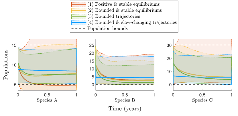
Figure S1: Median and 95% prediction interval populations for the three-species ecosystem model using each of the four sets of constraints.

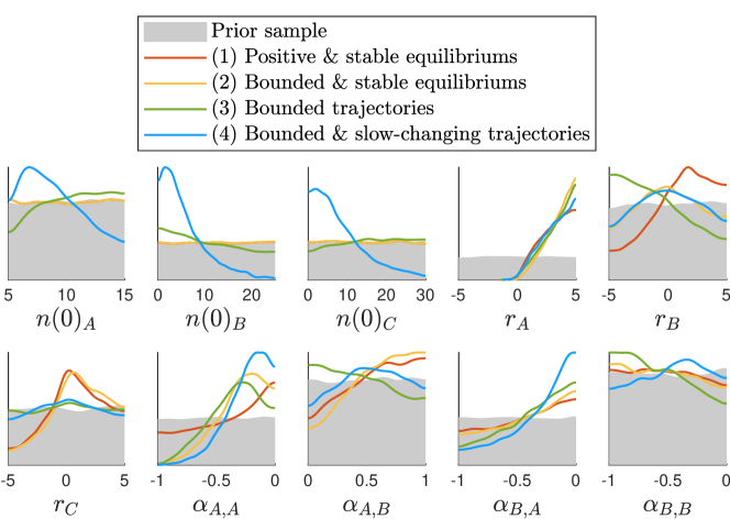
Figure S2: Estimated marginal parameter distributions of the three-species predator-prey ecosystem model when parameterised to each of the four sets of constraints.

Each of the four sets of constraints we analysed led to qualitatively different population trajectories (as shown for a simple three-species predator-prey ecosystem in Figure 1; full details of the ecosystem model provided in Supplementary Materials Section S.3.1). First, if the classic feasible and stable equilibrium-based constraints (constraint set 1 in Table 1) are used to generate ecosystem trajectories, the resulting steady state populations are not restricted, and can result in extremely large or small populations that do not necessarily adhere to “reasonable limits” that we may wish to enforce (Figure 1b row 1). Introducing limits to equilibrium populations (constraint set 2 in Table 1) can be used to force the long-term behaviour within some limits; however, populations can still exceed these before reaching equilibrium (Figure 1b, row 2). Instead, the non-equilibrium assumption that constrains trajectories to be within reasonable bounds (constraint set 3 in Table 1) removed any possibility of observing unrealistic population sizes for a period of interest (Figure 1b, row 3). Finally, in addition to constraining trajectories by population sizes, limiting the rate of population change (constraint set 4 in Table 1; Figure 1b, row 4) removes the chaotic fluctuations in populations that may be present in other sets of constraints where the rate of population change is not limited. Hence, the choice of constraints can drastically alter the population trajectories obtained for an ecosystem model. Beyond these individual trajectories, the constraint choice also affects predictions from an ensemble of trajectories (Figure S1) and the parameter estimates (Figure S2).

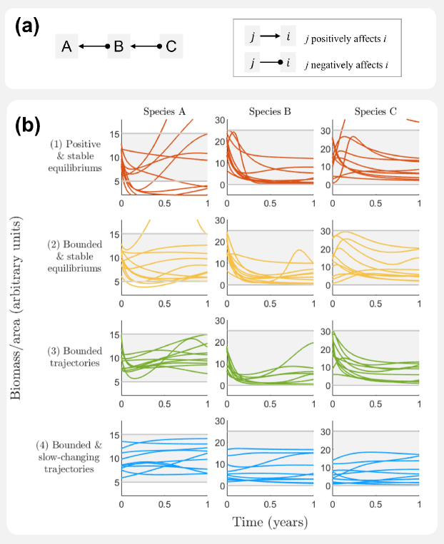
Figure 1: (a) The three-species predator-prey ecosystem network constructed into a Lotka-Volterra ecosystem model (see Supplementary Material Section S.3.1 for further detail). (b) Ten examples of population trajectories for the simple three-species ecosystem model obtained using each set of constraints. The shaded area between the grey lines indicates the expert-elicited “reasonable” population limits (see Supplementary Material Section S.3.1 for further detail). Notice that the choice out of the four sets of constraints can lead to considerably different population predictions.

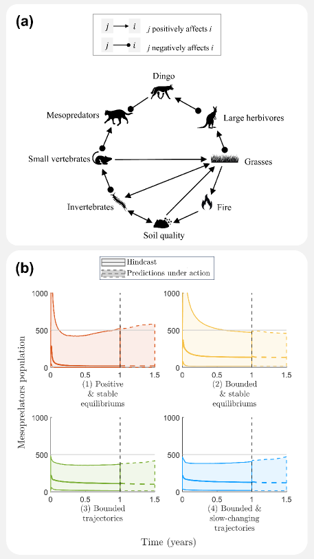
Figure 2: (a) A semiarid Australian ecosystem network simulated by a Lotka-Volterra ecosystem model (see Supplementary Material Section S.4.1 for further detail). (b) Predicted mesopredator population responses (median and 95% prediction interval) to removing 50% of the dingo population from the ecosystem using each set of constraints. Each ensemble of constraints was used to predict one year of population dynamics in the full ecosystem, then were used to predict population responses for the six month period following the pulse perturbation to dingoes. Notice that the choice of constraints affects both the projected populations and the responses to the management action, such that the populations are orders of magnitude different and reveal different trends.

2.2 Constraint choice drastically alters predicted management outcomes, illustrated by an eight-node semi-arid Australian ecosystem model

Vastly different population responses are obtained depending on the constraints used to model the ecosystem-wide effects of dingo regulation in semi-arid Australia ³⁶; ¹¹. Modelled populations (e.g., for mesopredators, Figure 2b) can change considerably based on the constraint choice, both for hindcasts (left of vertical dashed line) and in response to removing 50% of the dingoes (right of vertical dashed line). Figure 2b reveals that the modelled populations can be orders of magnitude different between constraints (e.g., the 95% prediction interval yields a maximum mesopredator population of approximately 2000 for set (1), compared to 500 for set (4)), and can show qualitatively different trends in response to dingo removal (e.g.  the 95% prediction interval indicates that in response to the action mesopredators populations may rise under set (1), but fall under set (2)). Such changes in the predicted effects of ecosystem management could ultimately lead decision-makers to different conclusions on the best management of an ecosystem. See Supplementary Material Section S.4.1 for further information on this case study.

2.3 Relatively stable ecosystem trajectories can easily be obtained without enforcing feasible and stable equilibrium populations

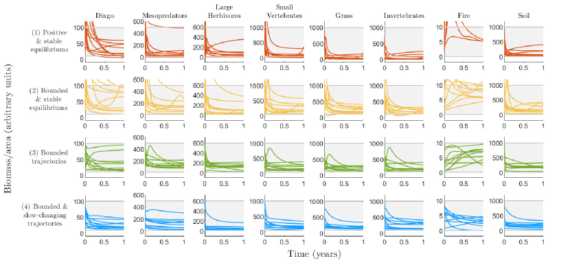
Figure S3: Comparison of some example trajectories produced by each set of constraints for the semiarid Australia ecosystem model.

Ensembles constrained by their non-equilibrium behaviour (constraint sets 3 and 4 in Table 1) exhibit reasonable slow-changing dynamics during the period of interest (Figure S3). For example, for the semiarid Australia ecosystem model (Figure 2a), roughly half of the trajectory-based ensembles (constraint sets (3) and (4) in Table 1) were either infeasible or unstable (Figure 3), which is potentially reasonable ecosystem behaviour that is simply not mathematically possible if equilibrium constraints are imposed (constraint sets (1) or (2) in Table 1). This indicates fundamental differences in the long-term behaviour of these parameterisations, and shows that trajectories which seem reasonable can also be infeasible and unstable.

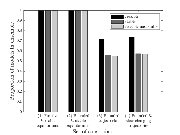
Figure 3: The proportion of parameter sets that have equilibrium behaviour that is feasible, stable or both for the semiarid Australia ecosystem model (Figure 2a; see Supplementary Material Section S.4.1 for further detail). Notice that the trajectory-based constraints lead to many parameterisations that are not feasible and stable.

2.4 Faster ecosystem generation using a new temporally-adaptive algorithm

Generation of ecosystem parameterisations that satisfy the trajectory-based constraints, can be slow, even when using the most recent SMC-EEM algorithm proposed for its computational efficiency ¹³, in one case taking over 81 hours on a high performance computer (Table S4; 12 parallel cores). However, the computation time can be cut using a new temporally adaptive version of this algorithm introduced in the present work (Methods Section 4.2). Put simply, our new algorithm initially simulates a shorter period when finding parameterisations that meet the constraints, and sequentially increases the simulation period until the full time period is covered (Figure 4a). The new temporally adaptive algorithm produces equivalent ensembles to the unaltered SMC-EEM algorithm (Figure 4b), whilst being up to four times faster (Table S4).

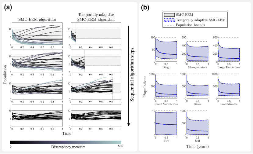
Figure 4: (a) A conceptual schema highlighting the differences between SMC-EEM (left) and temporally adaptive SMC-EEM (right). In this example, both algorithms aim to generate trajectories with populations in the grey area (arbitrary populations of 4-10). Each trajectory has an associated discrepancy measure, ranging from no discrepancy (black; trajectories meet constraints) to the maximum observed discrepancy (light blue; trajectories furthest from meeting constraints). From top to bottom, this figure shows that both algorithms iterate the trajectories closer to meeting the constraints, by sequentially reducing the discrepancy measures. The key difference is that SMC-EEM always simulates the full period (one unit of time). On the other hand, temporally adaptive SMC-EEM initially only simulates a small period (0.1 units of time) to rapidly eliminate trajectories that do not meet the constraints, and subsequently progresses the algorithm sequentially in time focusing on increasingly promising trajectories. (b) The population predictions for the semiarid Australian ecosystem model constrained using bounded trajectories (set (3) in Table 1; see Supplementary Materials Section S.4.1 for more information on this case study). Here we compare the median and 95% prediction intervals generated using both SMC-EEM (black) and temporally adaptive SMC-EEM (blue, dashed). Notice that both parameterisation algorithms produce similar forecasting distributions (see Supplementary Material Section S.4.3 for further comparison), yet the temporally adaptive algorithm is up to four times faster (Table S4).

3 Discussion

3.1 The argument for relaxing equilibrium assumptions when modelling ecological phenomena

Feasibility and stability conditions are ubiquitous in conservation modelling ¹²; ¹⁶ and in community ecology analyses ¹; ⁴; ⁷, despite concerns of whether the equilibrium perspective is appropriate for ecosystems ²³; ²⁵; ¹⁹. Given increasingly strong evidence and arguments against the concepts of ecological equilibrium and the “balance of nature” ideal ¹⁸, we argue in the present work that a reevaluation of coexistence ans stability in ecological networks is needed, and we introduce and demonstrate quantitative methods for how this can be achieved. This reevaluation does not yield trivial changes in projections – rather, drastic consequences of these assumptions are uncovered (see also Section 3.3), so we lay out here our justifications for the reevaluation of feasibility and stability conditions.

There is potentially a very large difference between the long-term equilibrium behaviour of an ecosystem and its current state ¹⁹; ²⁴, and this difference can lead to significantly different representations ²⁹ (Figures 1b, 2b, and S1-S4) and conservation practices ²⁵; ¹⁹ (Figure 2b) for an ecosystem. Ecosystems may never reach their long-term state; in fact, most time series data do not show evidence of an equilibrium state ²⁵, or cannot be distinguished from long transient behaviour ²⁰; ³⁰; ¹⁹. Therefore, representations of these ecosystems should seek to replicate the observable system behaviours without equilibrium assumptions, since many ecosystems that appear to be at equilibrium may instead be demonstrating long-transient behaviour ²¹; ²⁴; ¹⁹. In this work, we echo the sentiments of a growing body of literature which suggests that the equilibrium paradigm may not be appropriate for representing ecosystems ²⁵; ²¹; ²⁴; ²²; ¹⁹; ²³.

3.2 Field observations and/or expert knowledge should always fill the assumption gap

The arguments against ecological equilibria clearly raise concern about their persistent use in the literature. However, if making conclusions generally (e.g., Gellner et al. ³⁷) or if data is limited (e.g., Rendall et al. ¹²), some assumptions about ecosystem dynamics are necessary. We assert that this assumption gap should be filled not with equilibrium theory, but with readily available expert knowledge. The quantitative methods presented here (summarised in Table 1) provide a number of options for accomplishing this, depending on the available network information. Elicitation provides a fast and cheap way to input system knowledge ¹⁷. This information can be imperfect: it can contain biases ³⁸ and different experts may provide contradictory viewpoints (see e.g., Peterson et al. ¹⁶). However, any observed information can be of immense value, particularly when the alternative is to have no data ¹⁷; ³⁹.

The new methods we introduce here utilise (when available) expert-elicited upper and/or lower limits of population abundances, and upper limits on population rates of change. Information on equilibrium population limits can be elicited based on any knowledge of a species’ carrying capacity or by estimating minimum sustainable populations. Additionally, when considering trajectory-based constraints (set (3) or (4) in Table 1), then the estimated minimum and maximum abundance estimates for an observation period can be elicited, even though populations may have been historically higher or lower. Similarly, eliciting limits on population rates of change could be informed by ecological insights such as the maximum population growth (e.g., maximum eggs laid per year), or by whether sudden population changes have been observed (e.g., “for the last ten years of observation, we believe that populations have never halved over the period of a month”).

If this information cannot be confidently ascertained, conservative estimates can be provided (e.g., by multiplying best estimates by a factor of ten), limits can be left unspecified for certain species, or sensitivity analyses can be performed to identify if/when an estimate affects the represented system (this may be used to decide if further data collection is necessary; see Plein et al. ⁴⁰ Fig 3 for a similar analysis).

3.3 Towards using equilibrium-agnostic assumptions in practice

While the scientific consensus is gradually moving away from the equilibrium perspective ⁴¹, these ideas have not followed practice ²³; ²², due to the challenges of implementing transient theories in management ¹⁹. To our best knowledge, this is the first framework for parameterising transient ecosystem dynamics without time-series data. To illustrate our new framework, we developed three new ecosystem constraints (sets (2)-(4) in Table 1) as pragmatic alternatives to feasibility and stability for ecosystem modelling (set (1) in Table 1), two of which consider non-equilibrium behaviours.

When compared the classic feasible and stable equilibrium criteria (set (1)), introducing expert-informed limits on equilibrium populations (set (2)) can make equilibrium constraints more realistic by preventing models from stabilising on unreasonably large or small populations (Figure 1). While this constraint restricts equilibrium populations to a reasonable domain, population dynamics are unconstrained outside of the equilibrium dynamics, that may never be reached in nature ¹⁹; ²⁴. Therefore, for further constraints (set (3) and (4)), we instead consider population trajectories, regardless of whether they are at equilibrium or not; this choice to be equilibrium-agnostic is particularly appropriate as distinguishing equilibrium from non-equilibrium behaviour in time series data is a challenge in of itself ²⁰; ³⁰. This change to an equilibrium-agnostic perspective circumvents many of the issues associated with the equilibrium perspective: it replicates the observable ecosystem dynamics over the period the system has been managed; it allows for the possibility that the ecosystem may not be at or near equilibrium; and it does not restrict ecosystem behaviour outside the observation period (in case the observed system behaviour is e.g., a long transient ²¹).

Through limiting population trajectories to a reasonable population domain (set (3)), the strictness of assuming equilibrium behaviour is relaxed, such that ecosystem dynamics are reasonably constrained (Figure 1) without enforcing the equilibrium ideal (Figure 3). The population limits for trajectory-based constraints (sets (3) and (4)) define the populations that could reasonably have been expected during the observation period, hence they may be specified less conservatively than when constraining the theoretical equilibrium populations (set (2)). Finally, preventing impossible or unobserved population fluctuations (set (4)) can further ground these models in reality, such that the chaotic dynamics that ecosystem models can produce are only modeled during the observation period if experts agree it was possible (Figure 1). Overall, this process of redefining constraints has relaxed the equilibrium assumption such that constraints are equilibrium-agnostic, whilst increasing the restrictions on reasonable population dynamics using field knowledge.

The new constraints demonstrated in this work represent a starting point to a new way of thinking, rather than a definitive list of options for constraining ecosystem dynamics. System specific knowledge or data beyond those we have considered can always be available to further inform ecosystem models. Regardless, our results reveal that the choice of constraints can matter.

Predicted population trajectories can appear qualitatively different based on the constraints (Figure 1). Population hindcasts and predictions in response to conservation actions produced by ensembles can yield populations that are orders or magnitude different with different overall trends across different constraint sets (Figure 2). These differences can be so significant that it may lead to different conservation decision-making based on the framework chosen for modelling. Finally, we found that the choice of constraints could lead to entirely different long-term behaviour (Figure 3), such that population trajectories that appear reasonable according to our constraints are not capable of stable coexistence at equilibrium. While it is important to note that the impacts of this decision about constraints may depend on the ecosystem, the strictness of the constraint bounds chosen, and the model structure, we have shown that large differences in outcomes are possible. This has the potential for dramatic impact on the management of complex ecosystems, so motivates careful consideration of the models that represent these ecosystems and the confidence in any forecasted scenarios in these ecosystems ³⁵; ⁴².

3.4 Robust statistical frameworks drive advancements in simulation models and their connection to new data sources

Our novel framework connecting time series simulation models to expert knowledge in a statistically robust and efficient manner is useful beyond the ecological context discussed here. In this work, we exclusively demonstrated our methods on generalised Lotka-Volterra model structures because of its ubiquity in the field ⁴; ¹¹; ³⁵; however, any simulation model can be used. Any model that can produce species population trajectories can be used within this framework, including ordinary differential equation models, stochastic representations (see e.g., Ives et al. ⁴³) or spatial models. Additionally, in this work, we have emphasised that embedding expert-elicited information is invaluable where data is noisy, sparse or unavailable; but this statistical framework can use expert knowledge in conjunction with a myriad of other data sources. New, vast and high quality ecological data sources are constantly emerging as our technology advances, and robust statistical frameworks, such as this, are needed for combining these data with expert knowledge and mathematical representations.

As ecological modelling advances, statistical frameworks must not only be flexible to new data sources, but also efficient in the process that incorporates them. In switching from calculating equilibrium abundances to simulating population trajectories, the computational demands of generating ensembles can go from minutes to days (Table S4). Hence, the practical relaxation of equilibrium constraints, for realistic ecosystem networks, requires computational developments such as new statistical modifications to ensemble generation processes. In this work, we found that a temporally-adaptive modification of the present state-of-the-art model generation algorithm ¹³ could make the process up to four times faster (Table S4) without altering the results (Figure 4).

This temporal adaptation can enhance approximate Bayesian parameterisations of time series simulations in any context, and our novel framework can be generalised to incorporate expert knowledge beyond this ecological application. Modelling and simulation have become an integral part of understanding the world around us – from molecular systems ⁴⁴ to vast environmental domains ³³ – and new expert insights or ways to collect data constantly enhance our capability to predict what will happen in these systems ⁴⁵; ⁴⁶. Here, our desire to better represent ecosystems drives simultaneous improvement in computational techniques and statistical frameworks, benefiting ecology and quantitative science in general.

4 Methods

4.1 Choosing a set of assumptions for ecosystem modelling

For conservation modelling, we are typically interested in modelling populations through time. There are a multitude of suitable modelling frameworks (e.g., generalised Lotka-Volterra) that take the general form

$$\frac{\mathrm{d}n_{i}}{\mathrm{d}t}=f(n_{i}),\qquad i=1,\dots,N,$$ (1)

where $\frac{\mathrm{d}n_{i}}{\mathrm{d}t}$ is the change in population abundances $n_{i}(t)$ for ecosystem node $i$ over time $t$, $N$ is the number of ecosystem nodes being modelled, and $f$ is the functional form of the model. This model is specified by a set of parameters, whose values are chosen such that the resulting model meets the ecosystem constraints (e.g., feasible and stable equilibria). We describe four sets of assumptions that could be used for constraining parameter values for modelling ecosystems populations, and summarise these in Table 1 (Supplementary Material Section S.1 contains mathematical descriptions of each set of constraints).

4.1.1 Equilibria are feasible and stable

The first set of assumptions we consider are commonly used for conservation planning: feasible and stable equilibria ¹¹; ¹⁷; ¹⁴; ¹⁵; ¹²; ¹⁶. A model that satisfies these two constraints will have positive equilibrium populations, and local asymptotic stability.

Models which exhibit feasible and stable equilibria result in populations that tend toward positive populations, such that, population trajectories will eventually become attracted to the positive fixed point, or they will oscillate around these equilibrium values ²⁸; ⁴⁷. Hence, these models represent idealised long-term behaviour of ecosystems in the absence of any large external impacts: an ideal known as the “balance of nature” ¹⁸. However, these constraints place no restriction on the size of equilibrium populations and can yield extremely low or high equilibrium abundances.

4.1.2 Equilibria are bounded and stable

The condition of feasible equilibria requires the long-term populations of all species to be positive, but ecologists may wish to further restrict the possible abundances under equilibrium (e.g., limiting vegetation biomass to what is physically possible, or requiring a minimum invertebrate biomass to sustain an ecosystem). In addition to feasible and stable equilibria, this second set of constraints requires that equilibrium populations are within specified bounds for a subset of the species, where any unspecified bounds limit equilibria to positive values (feasibility).

Much like models constrained by feasible and stable equilibria, the resulting population trajectories for this set of constraints will stably approach or oscillate around a fixed point in population space in the long term. However, in this case, the fixed point is not only forced to be positive (feasible), but also within “reasonable” population limits.

This set of constraints may be advantageous to simply assuming feasibility and stability because any readily available information on reasonable populations can be included. However, as this is an equilibrium-based constraint, only the little-known long-term behaviour of the system is considered, and this may still allow unreasonable populations before the equilibrium is reached.

4.1.3 Trajectories are bounded

Next, we consider the population trajectories rather than the equilibrium behaviour of the system. The third constraint set requires population trajectories that exhibit finite coexistence, such that populations remain within bounds for a specified finite period of time $T$ (when simulated from a given set of initial conditions).

This constraint can be practically considered from the perspective of an ecosystem manager, who determines the minimum and maximum possible populations for their period of observation (e.g., “in the last 10 years there were 200-600 dingoes in the national park”). This approach assumes all species could persist for a period of time determined based on historical beliefs, rather than assuming species will indefinitely persist. Hence, feasibility is enforced for the period $T$, but beyond this extinctions are possible.

There are many arguments for why non-equilibrium approaches may be advantageous (see e.g., Oro and Martínez-Abraín ²⁵; Hastings et al. ²¹; Francis et al. ¹⁹), and this set of constraints allows modellers to parameterise non-equilibrium behaviour even without data. Since the stability of the system is no longer be assessed (as we do not consider the equilibrium behaviour), this set of constraints places no limitations on how rapidly populations can fluctuate.

4.1.4 Trajectories are bounded and slow-changing

Lastly, we impose restrictions on the rate of population change within the observation period (e.g., limiting population growth based on reproductive capabilities, or limiting population declines if crashes have not been observed). The fourth constraint set restricts population trajectories for the period $T$, such that both populations and the population rate of change are within specified bounds.

Again, this approach is targeted at what an ecosystem manager could observe: e.g., for the last 5 years, populations never halved or doubled in a month. Beyond the constrained period, species may go extinct or have explosive populations, hence we can think of this constraint as finite coexistence with “slow-changing” or “pseudo-stable” behaviour.

4.2 Generating samples that meet the constraints

For any given model structure, we aim to obtain a representative ensemble of parameter sets which meet the constraints (such that the ensemble provides a reasonable and well-balanced sample of all areas of parameter space that meet the constraints). Since this parameterisation process must be done without data, standard parameter inference techniques that require data cannot be applied. Instead, we use ideas from approximate Bayesian inference, where datasets are turned into summary statistics that are used for inference ³⁴; instead, in our case, the set of ecosystem constraints that must be satisfied are treated as summary statistics ¹³. To our best knowledge, only two approximate Bayesian sampling algorithms have been used for generating ensembles of ecosystem models to meet theoretical assumptions of ecosystem models. Firstly, an accept-reject algorithm that rejects any sampled parameter sets that do not satisfy all constraints has been used to find feasible and stable ecosystem models ¹¹ but this approach can be slow when there is a low probability of randomly sampling appropriate parameter values ¹³. Instead, the Sequential Monte Carlo ensemble ecosystem modelling (SMC-EEM) algorithm can be far more efficient at parameterising high-dimensional ecosystem networks to satisfy feasibility and stability constraints, while still producing a representative ensemble ¹³. Thus, below we summarise the SMC-EEM method, then introduce a new temporally adaptive extension of this method that provides an elegant solution for trajectory-based constraints.

4.2.1 SMC-EEM

The SMC-EEM algorithm uses information from rejected parameter sets to sequentially propose new values from a more informed distribution of potential parameter sets, rather than always using the prior distribution ¹³. The general idea, depicted in Figure 4a (left), is to iteratively reduce the measured “discrepancy” between the model simulations and ecosystem assumptions until the resulting ensemble of models all fully satisfy the enforced ecosystem constraints. For further details of the algorithm see Vollert et al. ¹³, and implementations are available in MATLAB ⁴⁸ and R ⁴⁹. While SMC-EEM is an efficient choice when the discrepancy is evaluated by analytically calculating the equilibrium, simulating full time series trajectories can add significant computation time, making SMC-EEM too slow to consider when trajectory-based constraints are present.

4.2.2 Temporally adaptive SMC-EEM

One downside of using SMC-EEM for trajectory-based constraints is that even if a trajectory has undesirable behaviour (and a very high discrepancy) in the early stages of the simulation, the full period $T$ is simulated, leading to wasted computation time. Instead, we propose a temporally adaptive modification of the SMC-EEM algorithm that avoids simulating the full time series by sequentially increasing, at each iteration $k$, the simulation time $t_{k}\leq T$, as more and more parameter sets are found that meet the constraints for the simulated period. Our new temporally adaptive SMC-EEM algorithm simultaneously decreases the discrepancy of model simulations from the constraints in the period $[0,t_{k}]$ and increases the simulation period $t_{k}$ towards the full time period $T$ (Figure 4a, right). Hence, we introduce and use the temporally adaptive SMC-EEM algorithm to generate ensembles of parameter sets for trajectory-based constraints in the present work. For details of the temporally adaptive SMC-EEM algorithm, see Supplementary Material Section S.2.

Data availability

The MATLAB code needed to replicate the results presented here is freely and publicly available on FigShare (DOI: 10.6084/m9.figshare.25679550).

Author contributions

SAV wrote the code and drafted the manuscript. SAV, CD and MPA designed the research, analysed the results, and edited the manuscript.

Supplementary materials

S.1 Further mathematical detail for constraint sets

S.1.1 Positive and stable equilibria

Feasibility and stability constrain the asymptotic (long-term) behaviour of the system. Hence, mathematically they are considered at the equilibrium population $n_{i}^{*}$ for each species $i$, obtained by solving

$$\frac{\mathrm{d}n_{i}^{*}}{\mathrm{d}t}=0,\qquad i=1,\dots,N,$$ (S1)

for the model defined by Equation (1) in the manuscript. Feasibility is achieved if these equilibrium populations are positive, $n^{*}_{i}>0$ for all species $i$ ⁷.

Stability – specifically local asymptotic stability – deals with the behaviour of the system when it is near this equilibria, hence the Jacobian matrix must be evaluated at the equilibrium populations $n_{i}^{*}$ to analyse stability:

$$J_{ij}=\left.\frac{\partial f_{i}}{\partial n_{j}}\right|_{n_{i}=n_{i}^{*}},$$ (S2)

where $J_{ij}$ is the $(i,j)$th element of the Jacobian matrix, and $f_{i}$ is the change in abundance for the $i$th node represented by the RHS of Equation (1) in the manuscript. A system is stable if the ecosystem populations will return to the equilibrium populations ⁷, such that the real part of all eigenvalues ($\lambda_{i}$) of the Jacobian matrix are negative, i.e. $\mathbb{R}\{\lambda_{i}\}<0,\ \forall i=1,...,N$.

S.1.2 Bounded and stable equilibria

In addition to stability, the equilibrium population $n_{i}^{*}$ of each species $i$ must be between $n_{i,\mathrm{min}}$ and $n_{i,\mathrm{max}}$ in its long-term dynamics (where $0\leq n_{i,\mathrm{min}}<n_{i,\mathrm{max}}$). These bounds are specified for each species in the system where it is appropriate to do so, and for the remaining species setting $n_{i,\mathrm{min}}=0$ and $n_{i,\mathrm{max}}=\infty$ is equivalent to the feasibility condition.

S.1.3 Bounded trajectories

Where the system must be simulated for a period of time, the initial populations $\bm{n}(0)$ are required to calculate population trajectories. We use the previously specified population bounds $n_{i,\mathrm{min}}$ and $n_{i,\mathrm{max}}$ to define a prior distribution for initial populations $\pi(n_{i}(0))\sim\mathcal{U}(n_{i,\mathrm{min}},n_{i,\mathrm{max}})$ and these initial conditions $\pi(n_{i}(0))$ are treated as parameters to be calibrated. Mathematically, the constraints will be satisfied if $n_{i,\mathrm{min}}<n_{i}(t)<n_{i,\mathrm{max}}$ for all species $i$ and for the full period time $t=(0,T)$, where $n_{0}$ are the initial conditions. Since the equilibrium behaviour is no longer considered, stability of the system is disregarded.

S.1.4 Bounded and slow-changing trajectories

The rate of change in species $i$ abundance per time step can be calculated as

$$R_{i}(t+\delta t)=\frac{\mathrm{d}n_{i}(t)/\mathrm{d}t}{n_{i}(t)}=\frac{n_{i}(t+\delta t)-n_{i}(t)}{n_{i}(t)\delta t},$$ (S3)

where $n_{i}(t)$ is the population of species $i$ at time $t$, and $\delta t$ is the change in time. By defining and measuring this rate of change, constraints can be enforced to limit this rate of change such that $R_{i,\mathrm{decrease}}<R_{i}(t+\delta t)<R_{i,\mathrm{increase}}$, where $R_{i,\mathrm{decrease}}$ is the negative rate of change limiting how quickly populations can decrease, and $R_{i,\mathrm{increase}}$ is the positive rate of change limiting how quickly populations can increase. For example, setting $R_{i,\mathrm{decrease}}=-0.5$ would indicate populations cannot reduce to 50% in one time step, and $R_{i,\mathrm{increase}}=0.5$ would mean populations cannot increase by 50% in one time step.) If it is inappropriate to limit the rate of change for a species $i$, the limits can be set as $R_{i,\mathrm{decrease}}=-\infty$ and $R_{i,\mathrm{increase}}=\infty$, such that any fluctuations will be allowed.

S.1.5 Summary of mathematical detail for each set of constraints

For each set of constraints, the mathematical description of the constraints and the measure used to calculate the discrepancy when using SMC-EEM are specified in Table S1.

Set of constraints	Description	Mathematical definition	Discrepancy measure $\rho(\bm{\theta})$ used in SMC-EEM
(1) Positive and stable equilibria	The long term behaviour of the system will have coexistence of all species, and will be able to recover from small changes to populations. The long term trajectories will be attracted towards a fixed set of positive populations, either reaching these populations or oscillating around them.	Equilibrium populations are positive, $\ n_{i}^{*}>0\ \ \forall i$, and stable, $\ \mathbb{R}(\lambda_{i})<0\ \ \forall i$.	$\displaystyle\sum_{i=1}^{N}\Bigl{[}$ $\displaystyle\max\{0,-n^{*}_{i}(\bm{\theta})\}$ $\displaystyle+\max\{0,\mathbb{R}\{\lambda_{i}\}\}\Bigr{]}$
(2) Bounded and stable equilibria	The long term behaviour of the system will have reasonable populations of all species, and will be able to recover from small changes to populations. The long term trajectories will be attracted towards a fixed set of reasonable populations, either reaching these populations or oscillating around them.	Equilibrium populations are within bounds, $\ n_{i,\mathrm{min}}\leq n_{i}^{*}\leq n_{i,\mathrm{max}}\ \ \forall i$, and stable, $\ \mathbb{R}(\lambda_{i})<0\ \ \forall i$.	$\displaystyle\sum_{i=1}^{N}\Bigl{[}$ $\displaystyle\max\{0,n^{*}_{i}(\bm{\theta})-n_{i,\mathrm{max}}\}$ $\displaystyle+\max\{0,n_{i,\mathrm{min}}-n^{*}_{i}(\bm{\theta})\}$ $\displaystyle+\max\{0,\mathbb{R}\{\lambda_{i}\}\}\Bigr{]}$
(3) Bounded trajectories	For a specified period of time, the population sizes will be reasonable without any constraints on the population dynamics. Beyond this period and for different species abundances, populations are not limited.	For $t=(0,T)$ populations are within bounds, $\ n_{i,\mathrm{min}}\leq n_{i}(t)\leq n_{i,\mathrm{max}}\ \ \forall i$.	$\displaystyle\sum_{i=1}^{N}\int_{t=0}^{T}\Bigl{[}$ $\displaystyle\max\{0,n_{i}(t,\bm{\theta})-n_{i,\mathrm{max}}\}\mathrm{d}t$ $\displaystyle+\max\{0,n_{i,\mathrm{min}}-n_{i}(t,\bm{\theta}\}\mathrm{d}t\Bigr{]}$
(4) Bounded and slow-changing trajectories	For a specified period of time, the population sizes will be reasonable and are limited by how rapidly they can increase or decrease. Beyond this period and for different species abundances, populations sizes and changes are not limited.	For $t=(0,T)$ populations are within bounds, $\ n_{i,\mathrm{min}}\leq n_{i}(t)\leq n_{i,\mathrm{max}}\ \ \forall i$ and the rate of population changes are within bounds, $\ R_{i,\mathrm{decrease}}\leq R_{i}(t)\leq R_{i,\mathrm{increase}}\ \ \forall i$.	$\displaystyle\sum_{i=1}^{N}\int_{t=0}^{T}\Bigl{[}$ $\displaystyle\max\{0,n_{i}(t,\bm{\theta})-n_{i,\mathrm{max}}\}\mathrm{d}t\,$ $\displaystyle+\max\{0,n_{i,\mathrm{min}}-n_{i}(t,\bm{\theta}\}\mathrm{d}t\,$ $\displaystyle+\max\{0,R_{i}(t,\bm{\theta})-R_{i,\mathrm{increase}}\}\mathrm{d}t\,$ $\displaystyle+\max\{0,R_{i,\mathrm{decrease}}-R_{i}(t,\bm{\theta})\}\mathrm{d}t\Bigr{]}$

Table S1: A detailed mathematical summary of each set of constraints.

S.2 Sequential Monte Carlo ensemble ecosystem modelling algorithms

Vollert et al. ¹³ introduced the SMC-EEM algorithm, based on sequential Monte Carlo - approximate Bayesian computation and provides a general overview, detailed algorithm and code. Here, we detail the temporally adaptive version of the algorithm by highlighting the differences from SMC-EEM in blue via an overview (Algorithm 1) and in full (Algorithms 2 and 3).

Within each iteration of the SMC-EEM algorithm (the black text in Algorithm 1), the ensemble of parameter sets are used to simulate the system (e.g., produce population trajectories), such that each parameter set can be attributed a discrepancy: a measure of how much the constraints were broken (e.g., how much above the upper bound did populations go). Using the collection of discrepancy scores, new parameter sets are proposed to reduce the discrepancy of simulations and iteratively approach an ensemble which meets all constraints.

INITIALISE

Define the discrepancy function as a measure of how much the constraints are exceeded, $\rho(\bm{\theta})$

Generate a sample from the prior distribution, $\pi(\bm{\theta})$ WEIGHT

Simulate the time series for each parameter set $\bm{\theta}$ for the period $(0,t_{0})$

Evaluate the discrepancy $\rho(\bm{\theta})$ for the simulation from $(0,t_{0})$

Set the initial discrepancy threshold $\epsilon_{0}$ such that a percentage of particles have $\rho<\epsilon_{0}$ while there are particles that break the constraints, $\max(\bm{\rho})>0$ OR the simulation time is less than the full period, $t_{k}<T$ do

       if there is a large portion of particles above the discrepancy threshold $\epsilon_{t}$ OR the simulation time is the full period $t_{k}=T$ then

             RESAMPLE

             Duplicate parameter sets based on their discrepancy ${\rho}$ to replace those with $\rho_{i}>\epsilon_{t}$

             MOVE

             Move each replaced parameter set using MCMC-ABC

       end if

       REWEIGHT

       Increase the simulation time based on the percentage of $\rho=0$, such that $t_{k}=\min\{t_{k-1}(1+n_{c}/M),T\}$ Simulate the time series for each parameter set for the period $(t_{k-1},t_{k})$

       Evaluate the discrepancy ${\rho}(\bm{\theta})$ for the simulation from $(0,t_{k})$

       Set the discrepancy threshold $\epsilon_{t}$, such that a percentage of particles have $\rho<\epsilon_{t}$

end while

Algorithm 1 Temporally adaptive SMC-EEM overview algorithm

INITIALISE

Define the discrepancy function as a measure of how much the constraints are exceeded, $\rho(\bm{\theta})$

Specify the prior distribution, $\pi(\bm{\theta})$

Select the tuning variables, including:

$\rightarrow$ The number of particles to be sampled, $M$

$\rightarrow$ The percentage of particles retained in each sequential step, $a$

$\rightarrow$ The desired probability of particles unmoved during MCMC-ABC, $c$

$\rightarrow$ The number of trial MCMC-ABC steps to gauge acceptance rate, $n_{\mathrm{MCMC}}$

$\rightarrow$ The initial period to simulate, $t_{k}=t_{0}$

$\rightarrow$ The maximum number of particles that can be kept when resampling, $b$

Generate a sample of $M$ particles ($\{\bm{\theta}_{i}\}_{i=1}^{M}$) from the prior distribution, $\pi(\bm{\theta})$ REWEIGHT

Simulate the systems defined by $\{\bm{\theta}_{i}\}_{i=1}^{M}$ for the period $(0,t_{k})$

Evaluate the discrepancy $\bm{\rho}=\{\rho(\bm{\theta}_{i})\}_{i=1}^{M}$ for the simulation from $(0,t_{k})$

Sort the particles $\bm{\theta}$ in ascending order of their corresponding discrepancy $\bm{\rho}$

Set the discrepancy threshold $\epsilon_{t}$ based on the number of particles to be retained $n_{\mathrm{keep}}=\lfloor a\times M\rfloor$ while there are particles that break the constraints, $\max(\bm{\rho})>0$ OR the simulation time is less than the full period, $t_{k}<T$ do

       if there are enough particles to drop, $n_{keep}<b$ OR the simulation time is the full period $t_{k}=T$ then

             RESAMPLE

             Transform current values of $\bm{\theta}$ to $\tilde{\bm{\theta}}$ such that the parameter-space is less restricted

             Duplicate retained particle values based on discrepancy $\bm{\rho}$ to replace those with $\rho_{i}>\epsilon_{t}$

             Calculate the sample covariance matrix, $\Sigma=cov(\{\bm{\theta}_{i}\}_{i=1}^{n_{\mathrm{keep}}})$ MOVE

             for each of the $n_{\mathrm{MCMC}}$ trial MCMC-ABC steps do

                   Move the particles using MCMC-ABC (Algorithm 3)

             end for

            Estimate the acceptance rate, $a_{t}$

             Determine the number of MCMC-ABC iterations to perform, $R_{t}=\lceil\log(c)/\log(1-a_{t})\rceil$

             for each of the remaining MCMC-ABC steps, $R_{t}-n_{\mathrm{MCMC}}$ do

                   Move the particles using MCMC-ABC (Algorithm 3)

             end for

            

       end if

       REWEIGHT

       Increase the simulation time based on the number of particles $n_{c}$ with no discrepancy, such that $t_{k}=\min\{t_{k-1}(1+n_{c}/M),T\}$

end while

Transform current values of $\tilde{\bm{\theta}}$ to $\bm{\theta}$ to simulate the system

Simulate the systems defined by $\{\bm{\theta}_{i}\}_{i=1}^{M}$ for the period $(t_{k-1},t_{k})$ (NOTE: $(0,t_{k-1})$ is already simulated)

Evaluate the discrepancy $\bm{\rho}=\{\rho(\bm{\theta}_{i})\}_{i=1}^{M}$ for the simulation from $(0,t_{k})$

Sort the particles $\bm{\theta}$ in ascending order of their corresponding discrepancy $\bm{\rho}$

Set the discrepancy threshold based on the number of particles to be retained, $\epsilon_{t}=\rho(\bm{\theta}_{n_{\mathrm{keep}}})$

if we are dropping particles which meet all constraints, $\rho(\bm{\theta}_{i})=0$ where $i>n_{\mathrm{keep}}$ then

       Adjust $n_{\mathrm{keep}}$ to retain all particles where $\rho(\bm{\theta}_{i})=0$

end if

Algorithm 2 Temporally adaptive SMC-EEM

for each particle $i$ in $\{\bm{\theta}_{i}\}_{i=n_{\mathrm{keep}}}^{M}$ do

       Propose a new set of parameter values ${\tilde{\bm{\theta}_{i}}}^{*}$ using a multivariate normal proposal distribution, ${\tilde{\bm{\theta}_{i}}}^{*}\sim N(\tilde{\bm{\theta}_{i}},\Sigma)$

       Calculate the prior probability ($\pi(\tilde{\bm{\theta}})$ for the transform space) of the current and proposed parameter values ($\tilde{\bm{\theta}_{i}}$ and ${\tilde{\bm{\theta}_{i}}}^{*}$)

       Transform the current and proposed parameter values ($\tilde{\bm{\theta}_{i}}$ and ${\tilde{\bm{\theta}_{i}}}^{*}$) in terms of $\bm{\theta}$

       Simulate the system defined by $\{\bm{\theta}_{i}^{*}\}$ for the period, $(0,t_{k})$

       Evaluate the discrepancy $\rho(\bm{\theta}_{i}^{*})$ for the simulation from $(0,t_{k})$

       Accept or reject a particle based on a Metropolis-Hastings acceptance probability $\alpha=\min\left(1,\pi(\tilde{\bm{\theta}}_{i}^{*})/\pi(\tilde{\bm{\theta}}_{i})\right)$, if within the discrepancy threshold, $\rho(\bm{\theta}_{i}^{*})\leq\epsilon_{t}$

end for

Algorithm 3 MCMC-ABC algorithm used within temporally adaptive SMC-EEM method (Algorithm 2)

S.3 Additional information for the three species predator-prey network

This section contains both additional details of the three-species ecosystem model (Section S.3.1) and comparisons between models produced using different sets of constraints (Section S.3.2).

S.3.1 Modelling details

The three species ecosystem network (depicted in Figure 1a in the main text) was modelled using the generalised Lotka-Volterra equations. The generalised Lotka-Volterra equations take the form

$$\frac{\mathrm{d}n_{i}}{\mathrm{d}t}=\left[r_{i}+\sum_{j=1}^{N}\alpha_{i,j}n_{j}(t)\right]n_{i}(t),$$ (S4)

where $n_{i}(t)$ is the abundance of the $i$th ecosystem node at time $t$, $r_{i}$ is the growth rate of the $i$th ecosystem node, $N$ is the number of ecosystem nodes being modelled, and $\alpha_{i,j}$ is the per-capita interaction strength characterising the effect of node $j$ on node $i$. Typically, an ecosystem network – which specifies the interactions between each species – are used to characterise whether each interaction is positive, negative or zero. For this three-species network, the associated ecosystem model is given by

$$\frac{\mathrm{d}n_{A}}{\mathrm{d}t} =r_{A}n_{A}-\alpha_{A,A}{n_{A}}^{2}+\alpha_{A,B}n_{B}n_{A},$$

$$\frac{\mathrm{d}n_{B}}{\mathrm{d}t} =r_{B}n_{B}-\alpha_{B,A}n_{A}n_{B}-\alpha_{B,B}{n_{B}}^{2}+\alpha_{B,C}n_{B}n_{C},$$

$$\frac{\mathrm{d}n_{C}}{\mathrm{d}t} =r_{C}n_{C}-\alpha_{C,B}{n_{C}}n_{B}-\alpha_{C,C}{n_{C}}^{2}$$

The modelling framework used to generate the results was the Lotka-Volterra equations, though any model structure which allows calculation of the equilibrium populations and stability can be used instead. The equilibrium population $n_{i}^{*}$ for each species $i$ is the solution to

$$\frac{\mathrm{d}n^{*}_{i}}{\mathrm{d}t}=r_{i}n^{*}_{i}+n^{*}_{i}\sum_{j=1}^{N}\alpha_{i,j}n^{*}_{j}=0,\quad\quad\quad\forall i=1,...,N.$$ (S5)

For this three-species model, this can be calculated as …

To determine if the equilibrium is stable first requires calculation of the Jacobian matrix, evaluated at equilibrium populations ${n}_{i}^{*}$,

$$J_{ij}=\left.\frac{\partial\left(r_{i}n_{i}+n_{i}\sum_{j=1}^{N}\alpha_{i,j}n_{j}\right)}{\partial n_{j}}\right|_{n_{i}=n_{i}^{*}},$$ (S6)

where $J_{ij}$ is the $(i,j)$th element of the Jacobian matrix. The dynamic system is considered locally asymptotically stable if the real part of all eigenvalues ($\lambda_{i}$) of the Jacobian matrix are negative, i.e. $\mathbb{R}\{\lambda_{i}\}<0,\ \forall i=1,...,N$.

Within this modelling framework, the following details were specified:

Item	Description	Choice
Ensemble size	The number of parameter sets to be generated that meet the constraints.	$M=10,000$
Prior distribution	A distribution of the initial belief of parameter values.	$r_{i}\sim U(-5,5),$
		$\alpha_{i,j}\sim U(0,1),$
		$\qquad\forall i,j={A,B,C}.$
Population bounds	The (hypothetical) expert-elicited population limits for each species.	$5\leq n_{\mathrm{A}}\leq 15,$
		$0\leq n_{\mathrm{B}}\leq 25,$
		$0\leq n_{\mathrm{C}}\leq 30.$
Simulation period	The observation period for trajectory-based constraints.	$T=1$
Population change bounds	The (hypothetical) expert-elicited limits on population rate of change	$-1\leq R_{A}\leq 1,$
		$-2\leq R_{B}\leq 2,$
		$-6\leq R_{C}\leq 6.$

Table S2: Modelling choices for the three-species predator-prey ecosystem case study.

S.3.2 Additional results comparing sets of constraints

S.4 Additional information for the semiarid Australia case study

This section contains both additional detail on the modelling of the semiarid Australia ecosystem model (Section S.4.1), additional comparison of the effects of different sets of constraints on the modelling (Section S.4.2), and additional results comparing SMC-EEM with temporally adaptive SMC-EEM (Section S.4.3).

S.4.1 Modelling details

The ecosystem model we consider for this example is the generalised Lotka Volterra model for the semiarid Australian ecosystem network (Figure 2a in the manuscript). For more details on the generalised Lotka Volterra equations and ecosystem networks see Supplementary Materials Section S.3.1 where we describe the process for the three-species predator-prey network.

Within this modelling framework, the following details were specified:

Item	Description	Choice
Ensemble size	The number of parameter sets to be generated that meet the constraints.	$M=50,000$
Prior distribution	A distribution of the initial belief of parameter values.	$r_{i}\sim U(-5,5),\ \ \forall i$
		$\alpha_{i,j}\sim U(0,1),\ \ \forall i,j.$
Population bounds	The (hypothetical) expert-elicited population limits for each species.	$10\leq n_{\mathrm{D}}\leq 100,$
		$10\leq n_{\mathrm{M}}\leq 500,$
		$10\leq n_{\mathrm{LH}}\leq 600,$
		$50\leq n_{\mathrm{SV}}\leq 1000,$
		$100\leq n_{\mathrm{G}}\leq 1000,$
		$100\leq n_{\mathrm{I}}\leq 1000,$
		$0\leq n_{\mathrm{F}}\leq 10,$
		$0\leq n_{\mathrm{S}}\leq 1000$
Simulation period	The observation period for trajectory-based constraints.	$T=1$
Population change bounds	The (hypothetical) expert-elicited limits on population rate of change	$R_{i,\mathrm{increase}}=12,\ \ \forall i$
		$R_{i,\mathrm{decrease}}=-36,\ \ \forall i.$

Table S3: Modelling choices for the semiarid Australian ecosystem network case study. Population limits for each ecosystem network node are indicated such that $D$ represents dingoes, $M$ represents mesopredators, $LH$ represents large herbivores, $SV$ represents small vertebrates, $G$ represents grasses, $I$ represents invertebrates, $F$ represents fires, and $S$ represents soil quality.

Using the ensembles parameterised using each set of constraints, we simulated the system for the observation period ($T=1$ year) then removed 50% of the dingo population, and simulated the resulting populations over the following six months ($T=1/2$ years).

S.4.2 Additional results comparing sets of constraints

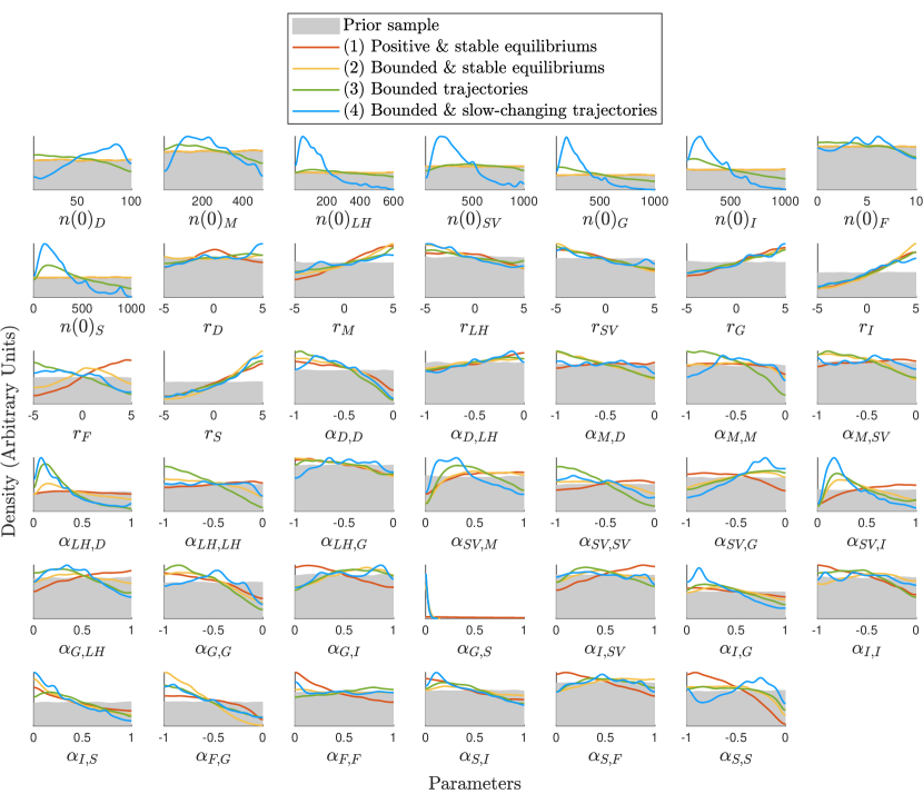
Figure S4: Estimated marginal parameter values for each set of constraints for the semiarid Australian ecosystem model.

S.4.3 Additional results comparing ensemble generation algorithms

The two different sampling algorithms – SMC-EEM and temporally adaptive SMC-EEM – were compared to assess whether the outputs of SMC-EEM were reproducible using temporally adaptive SMC-EEM. In addition to the comparison of predictive distributions (Figure 4b), we can compare the estimated marginal parameter values between SMC-EEM and the temporally adaptive version (see Vollert et al. ¹³ for a similar comparison).

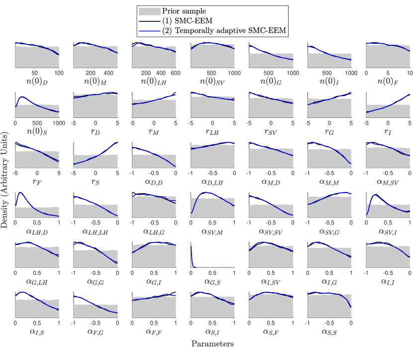
Figure S5: The estimated marginal parameter distributions for the semiarid Australia model, constrained using bounded trajectories (set 3). Here the outputs of SMC-EEM and temporally adaptive SMC-EEM are equivalent.

Set of constraints	Computation time (seconds)
	SMC-EEM	Temporally adaptive SMC-EEM
(1) Positive & stable equilibria	$70$	NA
(2) Bounded & stable equilibria	$1086$ ($\sim 18.1$ minutes)	NA
(3) Bounded trajectories	$12232$ ($\sim 3.4$ hours)	$6675$ ($\sim 1.9$ hours)
(4) Bounded & slow changing trajectories	$294582$ ($\sim 81.8$ hours)	$63841$ ($\sim 17.7$ hours)

Table S4: Computation times for generating 50000 parameter sets the semiarid Australia ecosystem model with each set of constraints. These ensembles were generated using the Queensland University of Technology’s high performance computers with 12 parallel cores.

References

- Allesina and Tang 2012 Stefano Allesina and Si Tang. Stability criteria for complex ecosystems. Nature, 483(7388):205–208, 2012.
- Barbier et al. 2021 Matthieu Barbier, Claire de Mazancourt, Michel Loreau, and Guy Bunin. Fingerprints of high-dimensional coexistence in complex ecosystems. Physical Review X, 11(1):011009, 2021.
- Donohue et al. 2016 Ian Donohue, Helmut Hillebrand, José M Montoya, Owen L Petchey, Stuart L Pimm, Mike S Fowler, Kevin Healy, Andrew L Jackson, Miguel Lurgi, Deirdre McClean, et al. Navigating the complexity of ecological stability. Ecology Letters, 19(9):1172–1185, 2016.
- Dougoud et al. 2018 Michaël Dougoud, Laura Vinckenbosch, Rudolf P Rohr, Louis-Félix Bersier, and Christian Mazza. The feasibility of equilibria in large ecosystems: A primary but neglected concept in the complexity-stability debate. PLoS Computational Biology, 14(2):e1005988, 2018.
- Gravel et al. 2016 Dominique Gravel, François Massol, and Mathew A Leibold. Stability and complexity in model meta-ecosystems. Nature Communications, 7(1):12457, 2016.
- Landi et al. 2018 Pietro Landi, Henintsoa O Minoarivelo, Åke Brännström, Cang Hui, and Ulf Dieckmann. Complexity and stability of ecological networks: a review of the theory. Population Ecology, 60:319–345, 2018.
- Grilli et al. 2017 Jacopo Grilli, Matteo Adorisio, Samir Suweis, György Barabás, Jayanth R Banavar, Stefano Allesina, and Amos Maritan. Feasibility and coexistence of large ecological communities. Nature Communications, 8(1):1–8, 2017.
- Song et al. 2018 Chuliang Song, Rudolf P Rohr, and Serguei Saavedra. A guideline to study the feasibility domain of multi-trophic and changing ecological communities. Journal of Theoretical Biology, 450:30–36, 2018.
- Stone 2018 Lewi Stone. The feasibility and stability of large complex biological networks: a random matrix approach. Scientific Reports, 8(1):1–12, 2018.
- Rohr et al. 2014 Rudolf P. Rohr, Serguei Saavedra, and Jordi Bascompte. On the structural stability of mutualistic systems. Science, 345(6195), 2014. doi: 10.1126/science.1253497.
- Baker et al. 2017 Christopher M Baker, Ascelin Gordon, and Michael Bode. Ensemble ecosystem modeling for predicting ecosystem response to predator reintroduction. Conservation Biology, 31(2):376–384, 2017.
- Rendall et al. 2021 Anthony R Rendall, Duncan R Sutherland, Christopher M Baker, Ben Raymond, Raylene Cooke, and John G White. Managing ecosystems in a sea of uncertainty: invasive species management and assisted colonizations. Ecological Applications, 31(4):e02306, 2021.
- Vollert et al. 2024a Sarah A Vollert, Christopher Drovandi, and Matthew P Adams. Unlocking ensemble ecosystem modelling for large and complex networks. PLoS Computational Biology, 20(3):e1011976, 2024a.
- Pesendorfer et al. 2018 Mario B Pesendorfer, Christopher M Baker, Martin Stringer, Eve McDonald-Madden, Michael Bode, A Kathryn McEachern, Scott A Morrison, and T Scott Sillett. Oak habitat recovery on California’s largest islands: scenarios for the role of corvid seed dispersal. Journal of Applied Ecology, 55(3):1185–1194, 2018.
- Peterson and Bode 2021 Katie Peterson and Michael Bode. Using ensemble modeling to predict the impacts of assisted migration on recipient ecosystems. Conservation Biology, 35(2):678–687, 2021.
- Peterson et al. 2021 Katie A Peterson, Megan D Barnes, Cailan Jeynes-Smith, Saul Cowen, Lesley Gibson, Colleen Sims, Christopher M Baker, and Michael Bode. Reconstructing lost ecosystems: A risk analysis framework for planning multispecies reintroductions under severe uncertainty. Journal of Applied Ecology, 58(10):2171–2184, 2021.
- Bode et al. 2017 Michael Bode, Christopher M Baker, Joe Benshemesh, Tim Burnard, Libby Rumpff, Cindy E Hauser, José J Lahoz-Monfort, and Brendan A Wintle. Revealing beliefs: using ensemble ecosystem modelling to extrapolate expert beliefs to novel ecological scenarios. Methods in Ecology and Evolution, 8(8):1012–1021, 2017.
- Cuddington 2001 Kim Cuddington. The “balance of nature” metaphor and equilibrium in population ecology. Biology and Philosophy, 16:463–479, 2001.
- Francis et al. 2021 Tessa B Francis, Karen C Abbott, Kim Cuddington, Gabriel Gellner, Alan Hastings, Ying-Cheng Lai, Andrew Morozov, Sergei Petrovskii, and Mary Lou Zeeman. Management implications of long transients in ecological systems. Nature Ecology & Evolution, 5(3):285–294, 2021.
- Boettiger 2021 Carl Boettiger. Ecological management of stochastic systems with long transients. Theoretical Ecology, 14(4):663–671, 2021.
- Hastings et al. 2018 Alan Hastings, Karen C Abbott, Kim Cuddington, Tessa Francis, Gabriel Gellner, Ying-Cheng Lai, Andrew Morozov, Sergei Petrovskii, Katherine Scranton, and Mary Lou Zeeman. Transient phenomena in ecology. Science, 361(6406), 2018.
- Wallington et al. 2005 Tabatha J Wallington, Richard J Hobbs, and Susan A Moore. Implications of current ecological thinking for biodiversity conservation: a review of the salient issues. Ecology and Society, 10(1), 2005.
- Mori 2011 Akira S Mori. Ecosystem management based on natural disturbances: hierarchical context and non-equilibrium paradigm. Journal of Applied Ecology, 48(2):280–292, 2011.
- Morozov et al. 2020 Andrew Morozov, Karen Abbott, Kim Cuddington, Tessa Francis, Gabriel Gellner, Alan Hastings, Ying-Cheng Lai, Sergei Petrovskii, Katherine Scranton, and Mary Lou Zeeman. Long transients in ecology: Theory and applications. Physics of Life Reviews, 32:1–40, 2020.
- Oro and Martínez-Abraín 2023 Daniel Oro and Alejandro Martínez-Abraín. Ecological non-equilibrium and biological conservation. Biological Conservation, 286:110258, 2023.
- Botkin 1990 Daniel B Botkin. Discordant harmonies: a new ecology for the twenty-first century. Oxford University Press, New York, 1990.
- Waltner-Toews et al. 2003 David Waltner-Toews, James J Kay, Cynthia Neudoerffer, and Thomas Gitau. Perspective changes everything: managing ecosystems from the inside out. Frontiers in Ecology and the Environment, 1(1):23–30, 2003.
- DeAngelis and Waterhouse 1987 Donald L DeAngelis and JC Waterhouse. Equilibrium and nonequilibrium concepts in ecological models. Ecological Monographs, 57(1):1–21, 1987.
- Hastings 2001 Alan Hastings. Transient dynamics and persistence of ecological systems. Ecology Letters, 4(3):215–220, 2001.
- Reimer et al. 2021 JR Reimer, J Arroyo-Esquivel, J Jiang, HR Scharf, EM Wolkovich, K Zhu, and C Boettiger. Noise can create or erase long transient dynamics. Theoretical Ecology, 14(4):685–695, 2021.
- Mouquet et al. 2015 Nicolas Mouquet, Yvan Lagadeuc, Vincent Devictor, Luc Doyen, Anne Duputié, Damien Eveillard, Denis Faure, Eric Garnier, Olivier Gimenez, Philippe Huneman, et al. Predictive ecology in a changing world. Journal of Applied Ecology, 52(5):1293–1310, 2015.
- Kristensen et al. 2019 Nadiah P Kristensen, Ryan A Chisholm, and Eve McDonald-Madden. Dealing with high uncertainty in qualitative network models using Boolean analysis. Methods in Ecology and Evolution, 10(7):1048–1061, 2019.
- Geary et al. 2020 William L Geary, Michael Bode, Tim S Doherty, Elizabeth A Fulton, Dale G Nimmo, Ayesha IT Tulloch, Vivitskaia JD Tulloch, and Euan G Ritchie. A guide to ecosystem models and their environmental applications. Nature Ecology & Evolution, 4(11):1459–1471, 2020.
- Sunnåker et al. 2013 Mikael Sunnåker, Alberto Giovanni Busetto, Elina Numminen, Jukka Corander, Matthieu Foll, and Christophe Dessimoz. Approximate Bayesian computation. PLoS Computational Biology, 9(1):e1002803, 2013.
- Adams et al. 2020 Matthew P Adams, Scott A Sisson, Kate J Helmstedt, Christopher M Baker, Matthew H Holden, Michaela Plein, Jacinta Holloway, Kerrie L Mengersen, and Eve McDonald-Madden. Informing management decisions for ecological networks, using dynamic models calibrated to noisy time-series data. Ecology Letters, 23(4):607–619, 2020.
- Newsome et al. 2015 Thomas M Newsome, Guy-Anthony Ballard, Mathew S Crowther, Justin A Dellinger, Peter JS Fleming, Alistair S Glen, Aaron C Greenville, Chris N Johnson, Mike Letnic, Katherine E Moseby, et al. Resolving the value of the dingo in ecological restoration. Restoration Ecology, 23(3):201–208, 2015.
- Gellner et al. 2023 Gabriel Gellner, Kevin McCann, and Alan Hastings. Stable diverse food webs become more common when interactions are more biologically constrained. Proceedings of the National Academy of Sciences, 120(31):e2212061120, 2023.
- Martin et al. 2012 Tara G Martin, Mark A Burgman, Fiona Fidler, Petra M Kuhnert, SAMANTHA Low-Choy, Marissa McBride, and Kerrie Mengersen. Eliciting expert knowledge in conservation science. Conservation Biology, 26(1):29–38, 2012.
- Kuhnert et al. 2010 Petra M Kuhnert, Tara G Martin, and Shane P Griffiths. A guide to eliciting and using expert knowledge in bayesian ecological models. Ecology Letters, 13(7):900–914, 2010.
- Plein et al. 2022 Michaela Plein, Katherine R O’Brien, Matthew H Holden, Matthew P Adams, Christopher M Baker, Nigel G Bean, Scott A Sisson, Michael Bode, Kerrie L Mengersen, and Eve McDonald-Madden. Modeling total predation to avoid perverse outcomes from cat control in a data-poor island ecosystem. Conservation Biology, 36(5):e13916, 2022.
- Moore et al. 2009 Susan A Moore, Tabatha J Wallington, Richard J Hobbs, Paul R Ehrlich, CS Holling, Simon Levin, David Lindenmayer, Claudia Pahl-Wostl, Hugh Possingham, Monica G Turner, et al. Diversity in current ecological thinking: implications for environmental management. Environmental management, 43:17–27, 2009.
- Botelho et al. 2024 Larissa Lubiana Botelho, Cailan Jeynes-Smith, Sarah Vollert, and Michael Bode. Ecosystem models cannot predict the consequences of conservation decisions. arXiv preprint arXiv:2401.10439, 2024.
- Ives et al. 2003 Anthony R Ives, Brian Dennis, Kathryn L Cottingham, and Stephen R Carpenter. Estimating community stability and ecological interactions from time-series data. Ecological monographs, 73(2):301–330, 2003.
- Schlick 2010 Tamar Schlick. Molecular modeling and simulation: an interdisciplinary guide, volume 2. Springer, 2010.
- Monsalve-Bravo et al. 2022 Gloria M Monsalve-Bravo, Brodie AJ Lawson, Christopher Drovandi, Kevin Burrage, Kevin S Brown, Christopher M Baker, Sarah A Vollert, Kerrie Mengersen, Eve McDonald-Madden, and Matthew P Adams. Analysis of sloppiness in model simulations: Unveiling parameter uncertainty when mathematical models are fitted to data. Science advances, 8(38):eabm5952, 2022.
- Ma’ayan 2017 Avi Ma’ayan. Complex systems biology. Journal of the Royal Society Interface, 14(134):20170391, 2017.
- Edelstein-Keshet 2005 Leah Edelstein-Keshet. Mathematical Models in Biology. SIAM, 2005.
- Vollert et al. 2024b Sarah A Vollert, Christopher Drovandi, and Matthew P Adams. Code repository for Unlocking ensemble ecosystem modelling for large and complex networks. https://figshare.com/articles/software/Code_repository_for_Unlocking_ensemble_ecosystem_modelling_for_large_and_complex_networks_/23707119, 2024b.
- Pascal 2024 Luz V Pascal. EEMtoolbox. https://github.com/luzvpascal/EEMtoolbox, 2024.
Acknowledgements
SAV is supported by a Queensland University of Technology Centre for Data Science, Australia Scholarship. CD is supported by an Australian Research Council Future Fellowship (FT210100260). MPA and SAV acknowledge funding support from an Australian Research Council Discovery Early Career Researcher Award (DE200100683). Computational resources were provided by the eResearch Office, Queensland University of Technology.