Conformal inference for random objects

Abstract

We develop an inferential toolkit for analyzing object-valued responses, which correspond to data situated in general metric spaces, paired with Euclidean predictors within the conformal framework. To this end we introduce conditional profile average transport costs, where we compare distance profiles that correspond to one-dimensional distributions of probability mass falling into balls of increasing radius through the optimal transport cost when moving from one distance profile to another. The average transport cost to transport a given distance profile to all others is crucial for statistical inference in metric spaces and underpins the proposed conditional profile scores. A key feature of the proposed approach is to utilize the distribution of conditional profile average transport costs as conformity score for general metric space-valued responses, which facilitates the construction of prediction sets by the split conformal algorithm. We derive the uniform convergence rate of the proposed conformity score estimators and establish asymptotic conditional validity for the prediction sets. The finite sample performance for synthetic data in various metric spaces demonstrates that the proposed conditional profile score outperforms existing methods in terms of both coverage level and size of the resulting prediction sets, even in the special case of scalar and thus Euclidean responses. We also demonstrate the practical utility of conditional profile scores for network data from New York taxi trips and for compositional data reflecting energy sourcing of U.S. states.

Keywords: Conditional distance profiles, Conformity score, Empirical process, Non-Euclidean data, Transport cost, Uniform convergence

1 Introduction

The conformal prediction framework was introduced by Vovk et al. (2005, 2009) as a sequential approach for forming prediction intervals. Subsequently, conformal inference has achieved notable success in various statistical settings, such as predictive inference for non-parametric regression (Lei et al., 2013; Lei and Wasserman, 2014; Lei et al., 2018; Chernozhukov et al., 2021; Barber et al., 2023), covariates shift problems (Barber et al., 2023; Gibbs and Candès, 2021, 2022), change point detection (Vovk et al., 2021), hypothesis testing (Vovk, 2021; Hu and Lei, 2023), outlier detection (Bates et al., 2023), time series (Angelopoulos et al., 2024; Yang et al., 2024) and survival analysis (Candès et al., 2023).

In the regression setting with training data $(X_{i},Y_{i})_{i=1}^{n}$ and additional identically and independently distributed (i.i.d.) sampled data $(X_{n+1},Y_{n+1})$, the aim of conformal prediction is to construct a prediction set $C_{\alpha}(X_{n+1})$ such that

$$\mathbb{P}({Y_{n+1}\in C_{\alpha}(X_{n+1})})\geq 1-\alpha.$$ (1)

To determine whether a value $y$ in the response space should be included in the prediction set $C_{\alpha}(X_{n+1})$, the basic idea of conformal prediction is to test the null hypothesis that $Y_{n+1}=y$ and to construct a valid $p$-value based on the empirical quantiles of a suitable score function that is evaluated for the sample $(X_{i},Y_{i}),\ldots,(X_{n},Y_{n}),(X_{n+1},y)$.

Besides marginal coverage (1), a more pertinent but also more ambitious and harder to achieve target is to require guaranteed coverage for each new instance rather than average coverage as conveyed by (1), i.e., to satisfy the conditional validity criterion

$$\mathbb{P}({Y_{n+1}\in C_{\alpha}(X_{n+1})|X_{n+1}})\geq 1-\alpha.$$ (2)

The left-hand side of equation (2) represents coverage conditional on the predictor $X_{n+1}$, while the marginal coverage (1) is defined by taking an additional expectation over $X_{n+1}$. In many real-world applications, conditional validity is the more satisfactory criterion since often one aims at predictions for a specific predictor level $X_{n+1}$, and averaging across all potential values of $X_{n+1}$ provides a lesser guarantee if one has $X_{n+1}$ in hand and is interested in prediction at this specific value of the predictor. However, conditional validity is hard to achieve and requires strong assumptions for the distribution of $(X,Y)$ (Vovk, 2012; Lei and Wasserman, 2014; Foygel Barber et al., 2021). A commonly adopted alternative is asymptotic conditional validity (Lei et al., 2018; Chernozhukov et al., 2021), i.e.,

$$\mathbb{P}({Y_{n+1}\in C_{\alpha}(X_{n+1})|X_{n+1}})\geq 1-\alpha+o_{P}(1).$$ (3)

A key feature of conformal inference is that the marginal coverage level (1) is always guaranteed as long as the score function meets certain symmetry conditions (Lei et al., 2018). However, the choice of the conformity score influences the size of the prediction sets and a well chosen score yields smaller prediction sets. In particular, Chernozhukov et al. (2021) utilized an adjusted conditional distribution function as conformity score and achieved an optimal prediction interval. However, their approach requires the optimization of a loss function involving the conditional quantile of $Y|X$, which becomes rather complicated when $Y|X$ is not unimodal. It is also worth noting that the optimality in Chernozhukov et al. (2021) specifically concerns prediction sets that comprise a single interval. In cases with bimodal conditional distributions, prediction sets featuring a union of distinct intervals are expected to be more efficient than those featuring a single interval. This observation motivated the adoption by Izbicki et al. (2022) of the conditional density as conformity score, and it was demonstrated that the resulting HPD-split conformal prediction sets have the smallest Lebesgue measure asymptotically.

One method to achieve conditional coverage is to partition the sample space $\mathcal{X}$ into distinct bins. For a new data point $X_{n+1}$, the model is fitted and conformity scores are evaluated solely within the sub-region containing $X_{n+1}$ (Lei and Wasserman, 2014; Izbicki et al., 2022). These approaches rely on the partitioning technique and specifically on the choice of tuning of parameters such as the number of bins. A general principle is to seek a conformity score that is approximately independent of $X$. The basic idea is straightforward: For any random variable $X$ with a distribution function $F$, the transformed variable $F(X)$ follows a uniform distribution on $(0,1)$, independently of $X$. Building on this idea, Chernozhukov et al. (2021) introduced the conditional cumulative distribution of $Y|X$ as conformity score and Izbicki et al. (2022) proposed the conditional density of $Y|X$ as score function.

Extending the scope of previous models for conformal prediction, we consider here a setting where the $Y_{i}$ are complex data objects that are situated in a general metric space $\mathcal{M}$ and the $X_{i}$ are Euclidean predictors. Object data residing in metric spaces paired with Euclidean predictors have found increasing interest in modern data analysis and various statistical approaches for analyzing such data have been developed over the last years. Statistical models for regression scenarios with object responses and Euclidean predictors have been studied for various scenarios, including responses located on a Riemannian manifold, which can be locally approximated by linear spaces (Chang, 1989; Fisher et al., 1993; Yuan et al., 2012; Fletcher, 2013; Cornea et al., 2017), responses that are distributions located in the Wasserstein space (Chen et al., 2023; Zhu and Müller, 2023) and also for responses in general metric spaces (Petersen and Müller, 2019; Lin and Müller, 2021). These previous studies either implicitly or explicitly developed models for object regression through implementations of conditional Fréchet means, thus focusing on the mean response.

For real-world data analysis, understanding the distribution of the responses given a covariate level is as important as quantifying the behavior of conditional means or Fréchet means when covariates vary. For example, regression models that only target conditional means are of little use when the underlying conditional distribution of a Euclidean response is not naturally centered around a single value, for example if it is bimodal. We extend the conformal framework to a new realm by introducing a conformity score that produces prediction sets of reasonably small size for all covariate levels, is sufficiently flexible to adapt to various response distributions, is efficient and, importantly, is easily computable for all types of responses that are situated in various non-Euclidean metric spaces.

Mapping object-valued data to linear spaces such as tangent spaces for the case of random objects situated on Riemannian manifolds is a familiar strategy to circumvent the absence of linear operations in metric spaces. However, available transformations are limited to responses that are situated in distributional and Riemannian spaces and do not cover other metric spaces. Another major limitation is that these linearizing maps are either metric-distorting or not bijective. In the latter case inverse maps that are necessary for the construction of prediction sets do not exist; various ad hoc work-arounds have been proposed, none of which is entirely satisfactory (Petersen and Müller, 2016; Bigot et al., 2017; Chen et al., 2023). More recently, new methods that operate intrinsically and do not rely on mapping to a linear space have been considered. These are more promising as they directly address the challenges of working within the non-Euclidean geometry of the response space (Dubey and Müller, 2020; Zhu and Müller, 2023). We adopt here such an intrinsic approach by adopting distance profiles (Dubey et al., 2024) for the proposed conformal inference. Distance profiles characterize the distributions of the distances of each element to a random object in the metric space. Distance profiles are determined by both the metric of the object space and its underlying probability measure and they characterize this measure if the metric is of strong negative type. Distance profiles correspond to one-dimensional distributions indexed by the elements $\omega$ of the metric space and form a well-defined stochastic process on the metric space. For the proposed extension of conformal inference, we introduce conditional distance profiles $F_{\omega|x}$, which characterize the inherent conditional distribution $Y|X=x$.

Statistical inference for object-valued data not only suffers from the absence of linear operations but also from the challenge that one does not have density functions, so that the density-based methods of Chernozhukov et al. (2021); Izbicki et al. (2022) are not feasible anymore. Note that as in the unconditional case $\{F_{\omega|x}:\omega\in\mathcal{M}\}$ is a family of one-dimensional distributions indexed by $\omega\in\mathcal{M}$ and $F_{Y|X=x}$ is a random measure when considering a random element $Y$ in the response space. Then the expected value of the 1-Wasserstein distance between $F_{Y|X=x}$ and $F_{\omega|X=x}$ characterizes the average transport cost of moving from $F_{Y|X=x}$ to $F_{\omega|X=x}$ and this motivates to employ conditional profile average transport costs (CPCs) to quantify the compatibility of a given element $\omega\in\mathcal{M}$ with the conditional distribution of $Y|X=x$. The heuristic is that less compatible elements should not be included in conditional prediction sets. Thus conditional profile costs serve as proxies for the unavailable conditional density function in general metric spaces and provide the starting point to arrive at conformal inference for object data by employing local linear estimators for both conditional distance profiles and conditional profile average transport costs. We derive uniform convergence rates, providing a solid theoretical foundation and show that these rates attain the optimal one-dimensional kernel smoothing rate when the metric space where responses reside has a polynomial covering number.

Employing this approach for conformal prediction leads to model-free statistical inference for object-valued responses coupled with Euclidean predictors when using a conditional profile score as conformity score, which we introduce here and that is defined as the distribution of conditional profile average transport costs. We then use the split conformal algorithm to derive prediction sets for object responses and show that these prediction sets lead to asymptotic conditional validity under mild assumptions. Conditional validity is also demonstrated via numerical experiments with synthetic data for various metric spaces. Even for the special Euclidean case where the responses are scalars, the proposed method consistently outperforms the HPD split approach (Izbicki et al., 2022) in both coverage levels and lengths of prediction sets for various settings. When dealing with multivariate predictors, local linear smoothing becomes increasingly problematic due to the curse of dimensionality. For this case we therefore replace local linear smoothing by single index Fréchet regression (Bhattacharjee and Müller, 2023), where one first obtains an estimate of a direction parameter and then projects the multivariate predictor onto this direction to obtain a single index predictor. Under mild assumptions on the consistency of the direction parameter the asymptotic conditional validity of the proposed conformity score remains valid.

To summarize, the main contributions of this paper are as follows. First, we introduce conditional distance profiles for random objects paired with Euclidean predictors. Second, we propose a novel conditional profile average transport cost and demonstrate its utility for statistical inference in general metric spaces. Third, we introduce the conditional profiles score, which is a new conformity score for general object responses situated in general metric spaces and paired with Euclidean predictors. Fourth, we show that this score achieves asymptotic conditional coverage under mild assumptions. Fifth, we develop a theoretical framework to establish uniform convergence rates for the local linear estimator involving indicator functions defined on metric spaces. Sixth, the efficiency of the conditional profile score is illustrated through comprehensive simulations and data applications across various metric spaces. Even for the classical case of scalar responses in $\mathbb{R}$ the proposed conditional profile score outperforms the HPD-score of Izbicki et al. (2022) in terms of both coverage levels and sizes of prediction sets. Data illustrations include networks for New York taxi trips and to compositional data reflecting energy usage by U.S. states as responses.

The paper is organized as follows. In Section 2, we introduce conditional distance profiles and conditional profile average transport costs. The main methods are presented in Section 3, including estimation procedures and the split conformal algorithm. Section 4 contains the main theoretical results; proofs and additional results can be found in the Supplement. The multivariate predictor case is discussed in Section 5. Numerical results for simulated data are presented in Section 6, and data applications in Section 7.

2 Conditional distance profiles

In what follows, we use $A_{n}=O_{p}(B_{n})$ to denote $\mathbb{P}(A_{n}\leq MB_{n})\geq 1-\epsilon$ and $A_{n}=o_{p}(B_{n})$ for $\mathbb{P}(A_{n}\leq\epsilon B_{n})\rightarrow 0$ as $n\rightarrow\infty$ for each $\epsilon>0$ and a positive constant $M=M(\epsilon)$. A non-random sequence $a_{n}$ is said to be $O(1)$ if it is bounded, and for each non-random sequence $b_{n}$, $b_{n}=O(a_{n})$ stands for $b_{n}/a_{n}=O(1)$ and $b_{n}=o(a_{n})$ stands for $b_{n}/a_{n}\rightarrow 0$. The relation $a_{n}\lesssim b_{n}$ indicates $a\leq\text{const}\cdot b$ for large $n$, and the relation $\gtrsim$ is defined analogously. We write $a_{n}\asymp b_{n}$ if $a_{n}\lesssim b_{n}$ and $b_{n}\lesssim a_{n}$. For $a\in\mathbb{R}$, we use $\lfloor a\rfloor$ to denote the largest integer smaller or equal to $a$. We write $\mathcal{L}^{2}(\mathcal{D}):=\{f:\,\,\mathcal{D}\mapsto\mathbb{R}:\,\,\int_{\mathcal{D}}f^{2}(x)dx<\infty\}$ for the space of square-integrable functions on $\mathcal{D}$, $\|f\|_{2}^{2}:=\int_{\mathcal{D}}f(s)^{2}ds$, and $\|f\|_{\infty}:=\sup_{s\in\mathcal{D}}|f(s)|$.

Consider a random pair $Z=(X,Y)\in\mathcal{X}\times\mathcal{M}$, where $\mathcal{X}$ is a compact subset of $\mathbb{R}^{d}$ and $\mathcal{M}$ is a totally bounded, separable metric space with the associated distance function $d(\cdot,\cdot)$. Given a probability space $(\Omega,\mathcal{O},\mathbb{P})$, where $\mathcal{O}$ represents the Borel $\sigma$-algebra on the domain $\Omega$ and $\mathbb{P}$ is a probability measure, the random pair $Z$ can be described as a measurable mapping $Z:\,\,\Omega\to\mathbb{R}^{d}\times\mathcal{M}$. The joint law of $(X,Y)$ is represented by $\mathbf{P}_{Z}$, such that $\mathbf{P}_{Z}(A)=\mathbb{P}(s\in\Omega:\,\,Z(s)\in A)$ for any Borel measurable set $A\subset\mathbb{R}^{d}\times\mathcal{M}$. We denote the marginal laws of $X$ and $Y$ as $\mathbf{P}_{X}$ and $\mathbf{P}_{Y}$, respectively. We also assume the conditional probability measure $\mathbf{P}_{Y|x}$ of $Y$ given $X=x$ exists, where $Y$ is the object response and $X$ a Euclidean predictor. We aim at inference for $Y$ given $X$, first focusing on the case of a one-dimensional predictor where $d=1$ in Section 3, while multivariate predictors are studied in Section 5.

For any $x\in\mathcal{X}$ and $\omega\in\mathcal{M}$, let $F_{\omega\mid x}$ represent the cumulative distribution function (CDF) of the distance between $\omega$ and the response $Y$, conditional on $X=x$ and with respect to $\mathbf{P}_{Z}$. We refer to the $F_{\omega\mid x}$ as conditional distance profiles,

$$F_{\omega\mid x}(t)=\mathbb{P}(d(\omega,Y)\leq t|X=x),\ \text{for all }t\in\mathbb{R}^{+}.$$ (4)

These conditional distance profiles can be seen as extensions of the previously introduced distance profiles $F_{\omega}(t)=\mathbb{P}(d(\omega,Y)\leq t)$ (Dubey et al., 2024) and related concepts (Wang et al., 2023); they serve to indicate the centrality of an element $\omega$; if $\omega$ is centrally located given $X=x$, its corresponding profile $F_{\omega\mid x}(t)$ will have relatively larger values near $t=0$ compared to the profiles of less centrally located elements $\omega\in\mathcal{M}$.

We may view $F_{\omega\mid x}(t)$ as an element in the Wasserstein space of distributions with positive domain,

$$\mathcal{W}:=\,\left\{\mu\in\mathcal{P}(\mathbb{R}^{+}):\,\,\int_{\mathbb{R}^{+}}x^{2}{\rm d}\mu(x)<\infty\right\},$$

where $\mathcal{P}(\mathbb{R}^{+})$ is the set of all probability measures on $\mathbb{R}^{+}$, equipped with the $p$-Wasserstein metric $d_{W,p}(\cdot,\cdot)$, which for $\mu,\nu\in\mathcal{W}$ is defined as

$$d_{W,p}(\mu,\nu):=\,\inf\left\{\left(\int_{\mathbb{R}^{+}\times\mathbb{R}^{+}}|x_{1}-x_{2}|^{p}{\rm d}\Gamma(x_{1},x_{2})\right)^{1/p}:\,\,\Gamma\in\Gamma(\mu,\nu)\right\}\quad\text{for }p>0,$$ (5)

where $\Gamma(\mu,\nu)$ is the set of joint probability measures on $\mathbb{R}^{+}\times\mathbb{R}^{+}$ with $\mu$ and $\nu$ as marginal measures. The Wasserstein space $(\mathcal{W},d_{W,p})$ is a separable and complete metric space (Ambrosio et al., 2008; Villani et al., 2009). The emerging field of distributional data analysis frequently utilizes the Wasserstein metric for one-dimensional distributions (Petersen and Müller, 2016; Petersen et al., 2022; Chen et al., 2023). We write $F^{-1}(u)=\inf\{x\in\mathbb{R}:\,\,F(x)\geq u\}$ for $u\in(0,1)$ to represent quantile functions and consider both $F_{\omega\mid x}$, $F^{-1}_{\omega|x}$ as representations of the probability measure $\mu_{\omega|x}$.

Given $X=x$, the conditional distance profile $F_{Y|x}$ can be regarded as a random element of $\mathcal{W}$, since it is indexed by the random element $Y\in\mathcal{M}.$ For any $\omega\in\mathcal{M}$, if $F_{\omega\mid x}$ is absolutely continuous with respect to the Lebesgue measure, the optimal transport map $F^{-1}_{Y|x}\circ F_{\omega\mid x}$ is the push-forward map from $F_{\omega\mid x}$ to $F_{Y|x}$. The integral

$$d_{W,1}(F_{Y|x},F_{\omega|x})=\int_{\mathbb{R}^{+}}\left|F^{-1}_{Y|x}\circ F_{\omega\mid x}(u)-u\right|{\rm d}F_{\omega\mid x}(u)$$

represents the 1-Wasserstein distance between $F_{\omega\mid x}$ and $F_{Y|x}$, and quantifies the amount of mass that needs to be moved from $F_{\omega\mid x}$ to arrive at $F_{Y|x}$, i.e., the transport cost. The connection between this transport cost and the conditional distance profiles is as follows.

Proposition 1.

For all $x_{1},x_{2}\in\mathcal{X}$ and $\omega_{1},\omega_{2}\in\mathcal{M}$, if $F_{\omega_{1}|x_{1}}(u)$ or $F_{\omega_{2}|x_{2}}(u)$ is continuous in $u$,

$$\int_{0}^{1}\left|F^{-1}_{\omega_{1}|x_{1}}(u)-F^{-1}_{\omega_{2}|x_{2}}(u)\right|{\rm d}u=\int_{{\mathbb{R}}^{+}}\left|F_{\omega_{1}|x_{1}}(u)-F_{\omega_{2}|x_{2}}(u)\right|{\rm d}u.$$

When the domain of the two cumulative distribution functions (CDFs) $F$ and $G$ is $[0,1]$, the equality $\int_{0}^{1}|F(u)-G(u)|{\rm d}u=\int_{0}^{1}|F^{-1}(u)-G^{-1}(u)|{\rm d}u$ is straightforward by the Fubini theorem. However, it is less obvious when this does not hold, and the proof of Proposition 1 utilizes the definition of conditional distance profiles, a change of variables, and the Fubini Theorem; details are in the supplement. Under the assumption that $F_{\omega_{2}|x_{2}}(u)$ is continuous, for the 1-Wasserstein distance, by Proposition 1,

$$d_{W,1}(F_{Y|x},F_{\omega|x})=\int_{0}^{1}\left|F^{-1}_{Y|x}(u)-F^{-1}_{\omega|x}(u)\right|{\rm d}u=\int_{0}^{\infty}\left|F_{Y|x}(u)-F_{\omega|x}(u)\right|{\rm d}u,$$

and this motivates

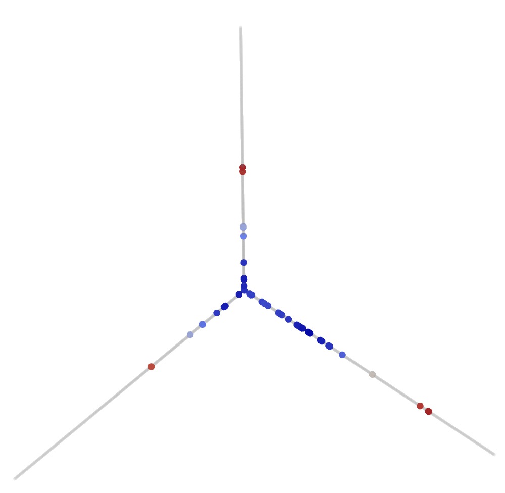
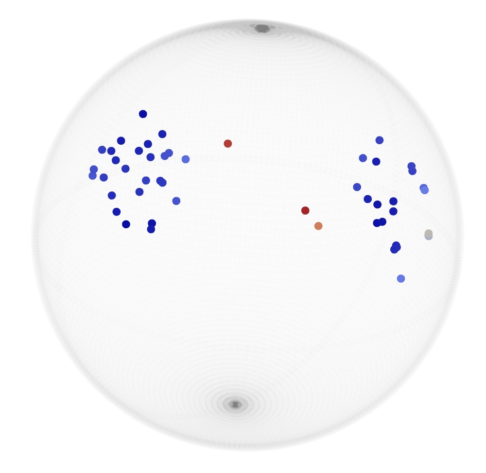
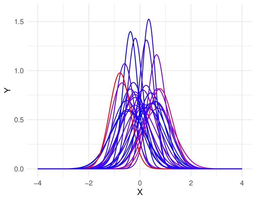
Figure 1: Illustration of the proposed profile average transport costs for data points generated for various metric spaces. The transition from low to high CPCs (6) is indicated by the color gradient from blue to red, where red indicates high values of profile average transport costs, while blue indicates low values. The left panel shows data in the tree space $\mathbb{T}^{3}$ with the BHV metric; each axis represents a distinct tree topology, and the position on the axis reflects the length of the interior edge. The middle panel shows data points that follow a distribution on $\mathbb{S}^{2}$, which is characterized by two modes centered at $\mu_{1}=(1,0,0)$ and $\mu_{2}=(0,1,0)$, each with equal probability 0.5. The data points are generated from the exponential map at $\mu_{k}$, applied to a random vector $V_{k}$. Here $V_{1}=(0,\epsilon_{1},\epsilon_{2})$ and $V_{2}=\epsilon_{3},0,\epsilon_{4})$, where $\epsilon_{1},\dots,\epsilon_{4}$ are r.v.s drawn from $\mathcal{N}(0,0.2)$. The right panel refers to data from the 2-Wasserstein space. Each curve represents the density function of a normal distribution $\mathcal{N}(\mu,\sigma))$, where $\mu$ and $\sigma$ are drawn from uniform distributions $\operatorname{Unif}(-0.8,0.8)$ and $\operatorname{Unif}(0.25,0.75)$.

the concept of conditional profile average transport cost (CPC),

$$C(\omega|x)=\,\mathbb{E}\left[\int_{\mathbb{R}^{+}}\left|F_{\omega\mid X}(t)-F_{Y|X}(t)\right|\,\mathrm{d}t\,\Bigm{|}X=x\right].$$ (6)

A low value of $C(\omega|x)$ means that the average transport cost for moving from $F_{\omega|x}$ to $F_{Y|x}$ is relatively small, indicating that $\omega$ has a high degree of centrality within the distribution $Y|X=x$. Figure 1 illustrates the proposed CPCs, conditional on a fixed $X=x$, for three metric spaces: The tree space $\mathbb{T}^{3}$ with the BHV metric, the sphere $\mathbb{S}^{2}$ with the geodesic metric and the 2-Wasserstein space $\mathcal{W}_{2}$ of distributions.

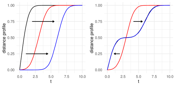
Figure 2: Distance profiles for normal and mixture normal distributions of $\mathcal{M}=\mathbb{R}$. The underlying distribution is normal $\mathcal{N}(3,1)$ for the left panel and a mixture of normals $0.5\mathcal{N}(-3,1)+0.5\mathcal{N}(3,1)$ for the right panel. Black, red, and blue lines represent the estimated distance profiles at $\omega=3,0,-3$, respectively. Arrows indicate the direction of transport of distance profiles, moving from the most central to the outermost point as determined by $\mathcal{H}(\omega|x_{0})$. In the right panel, the black and blue lines overlap for the most part.

Here CPCs are based on conditional expectations, unlike previously introduced unconditional transports and ranks (Dubey et al., 2024) that can also serve as a centrality measure. These transports and derived ranks can also be defined conditionally,

$$\mathcal{H}(\omega|x)=\,\mathbb{E}\left[\int_{0}^{1}\left\{F_{Y|X}^{-1}(u)-F_{\omega|X}^{-1}(u)\right\}\mathrm{d}u\Bigm{|}X=x\right].$$ (7)

Given $X=x_{0}$, for a distribution $Y|X=x_{0}$ that is symmetric around a central point $\omega_{0}$, the integral in Equation (7) with $\omega=\omega_{0}$ can be expected to be relatively large and $\mathcal{H}(\omega|x_{0})$ to decrease as the distance $d(\omega_{0},\omega)$ increases. The left panel of Figure 2 displays estimators for the distance profiles $F_{3|x_{0}}(t)$, $F_{0|x_{0}}(t)$, and $F_{-3|x_{0}}(t)$, corresponding to the conditional distribution $Y|X=x_{0}\sim\mathcal{N}(3,1)$. In this scenario, $\omega_{0}=3$ represents the most central point, with mass transferring from $F_{\omega_{0}|x_{0}}(t)$ to $F_{\omega|x_{0}}(t)$ from left to right for all $t>0$ and $\omega\neq\omega_{0}$. However, when the underlying distribution of $Y|X=x_{0}$ is not centered around a single point, the most central point as determined by Equation (7) may not always be the most pertinent choice. For instance, consider a mixture of normal distributions $Y|X=x_{0}\sim 0.5\mathcal{N}(-3,1)+0.5\mathcal{N}(3,1)$; the right panel of Figure 2 illustrates estimators for distance profiles $F_{3|x_{0}}(t)$, $F_{0|x_{0}}(t)$, and $F_{-3|x_{0}}(t)$. By symmetry, $F_{3|x_{0}}(t)=F_{-3|x_{0}}(t)$ for all $t>0$. Notably, mass transfers from $F_{0|x_{0}}(t)$ to $F_{3|x_{0}}(t)$ (or $F_{-3|x_{0}}(t)$) proceed from right to left for $t\in(0,3)$ and from left to right for $t\in(3,\infty)$. Since the centrality measure $\mathcal{H}(\omega|x_{0})$ reflects the difference between rightward and leftward moving mass, rather than the total transport cost, at the global center of the data, $\omega_{0}=0$, positioned between the two modes, the integral in Equation (7) reaches its maximum and decreases as $\omega$ moves away from $\omega_{0}$. However, in bimodal settings, this global center is less pertinent and statistical inference that adapts to the mixture distribution is preferable. The proposed average transport cost criterion performs much better in bimodal cases, as illustrated in Figure 4 of Section 3.1 below.

3 Conformal inference for object data

3.1 Conformal prediction with profile transport costs

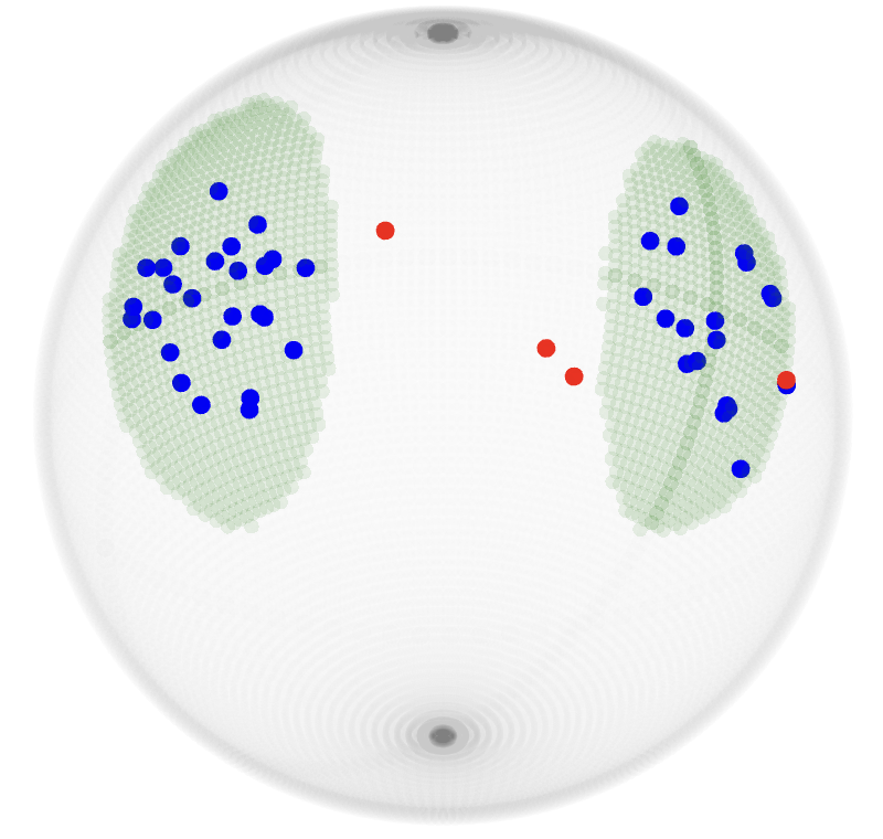
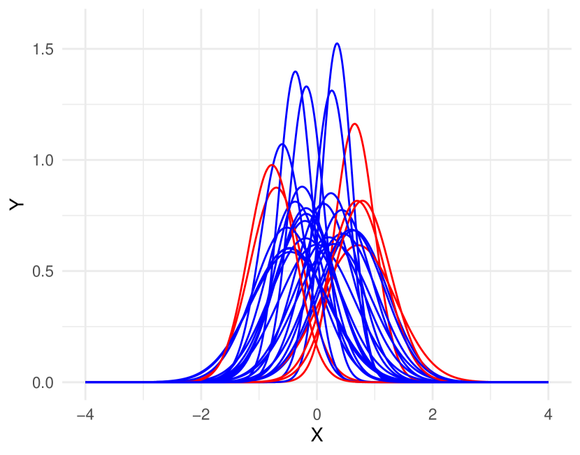
Figure 3: Illustration of conformal sets using conditional profile scores based on the data from Figure 1. The blue points (curves) represent the training data falling within the 90% prediction set, while the red points (curves) denote those that fall outside the 90% prediction set. In the left and middle panels, the estimated prediction sets are highlighted in green.

Given i.i.d. observations $(X_{i},Y_{i})\in\mathcal{X}\times\mathcal{M}$ for $i=1,\cdots,n$, we aim to predict $Y_{n+1}$ using the information from a future predictor $X_{n+1}$. In contrast to standard regression methods that correspond to versions of Fréchet regression in the scenario with random object responses and focus on the conditional Fréchet mean, our goal is to construct a prediction set $\hat{C}_{\alpha}(X_{n+1})$ that ensures asymptotic conditional validity (3) for a specified miscoverage level $\alpha$. The collection of prediction sets $\hat{C}_{\alpha}:=\{\hat{C}_{\alpha}(x):\,\,x\in\mathcal{X}\}$ is referred to as the $\alpha$-level prediction set.

The selection of a good score function is crucial for the effectiveness of conformal inference methods. A well-chosen score not only yields a smaller prediction set but also achieves asymptotic conditional validity. Note that for any random variable $X$ with a distribution function $F$, the transformed variable $F(X)$ follows a uniform distribution over the interval $(0,1)$ and is independent of $X$. Building on this, Chernozhukov et al. (2021) proposed $F(Y,X)$ as the conformity score, where $F(y,x)=\mathbb{P}(Y\leq y|X=x)$ represents the conditional CDF of $Y$ for a given $X=x$. Similarly, Izbicki et al. (2022) proposed the HPD-split score $H(f(Y|X)|X)$, where $f(y|x)$ is the conditional density function of $Y$ given $X=x$ and $H(z|x)=\mathbb{P}(f(Y|X)\leq z|X=x)$ denotes the conditional CDF of $f(Y|X)$ for a given $X=x$.

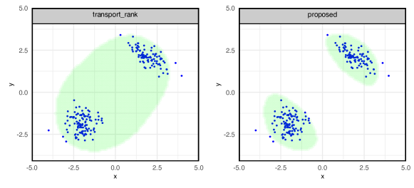
Figure 4: Conformal prediction sets generated using transport ranks (Dubey et al., 2024) as conformity score (left panel) and the proposed conditional profile scores defined in Equation (8) (right panel), for $\mathcal{M}=\mathbb{R}^{2}$. The training data are from a 2-dimensional Gaussian mixture, $0.5\mathcal{N}(\bm{\mu}_{1},\bm{\Sigma}_{1})+0.5\mathcal{N}(\bm{\mu}_{2},\bm{\Sigma}_{2})$, where $\bm{\mu}_{1}=(2,2)^{\top}$, $\bm{\mu}_{2}=(-2,-2)^{\top}$, $\bm{\Sigma}_{1}=(0.5,-0.3;-0.3,0.3)$ and $\bm{\Sigma}_{1}=(0.5,0;0,0.3)$. The data in the training set are blue, and the respective 90% conformal sets are shaded in green.

As discussed in Section 2, the conditional profile average transport costs (6) can be viewed as a centrality measure relating to the conditional probability measure on the object space. It is then straightforward to use the profile average transport costs as conformity score. However, this approach does not guarantee conditional coverage in general. Instead, we introduce the conditional profile score (CPS) as conformity score for random objects. The CPS corresponds to the conditional distribution of profile average transport costs,

$$S(z|x):=\,\mathbb{P}(C(Y|X)\leq z|X=x).$$ (8)

This choice is motivated by the example in Figure 3, which illustrates the conformal sets derived using the proposed conditional profile average transport costs (8) as conformity scores for the data in Figure 1, conditional on a specific $X=x$. Note that the generated conformal prediction sets aptly provide conformal inference for both unimodal and bimodal structures across different metric spaces.

An alternative is to use conditional transport ranks (Dubey et al., 2024) as conformity score. Based on (7), unconditional transport ranks are obtained as

$$R(\omega)=\hbox{expit}\left(\mathbb{E}\left[\int_{0}^{1}\{F^{-1}_{Y}(u)-F^{-1}_{\omega}(u)\}\,du\right]\right),$$ (9)

where $\hbox{expit}(x)=\frac{e^{x}}{1+e^{x}}$. The transport ranks $R(\omega)$ quantify the aggregated preference of $\omega$ in relation to the data distribution, where a larger $R(\omega)$ indicates that $\omega$ is more centrally located within the distribution. However, as illustrated in Figure 2, $R(\omega)$ is less suited to serve as a conformity score, which is evident when the underlying distribution is not centered around a single element. In the example in Figure 4, the conformal set determined by transport ranks as conformity scores is centered at the global center of the data, It is seen to be quite suboptimal for a 2-dimensional mixture Gaussian distribution. In contrast, the proposed CPS successfully distinguishes the two groups and leads to smaller prediction sets.

3.2 Estimation and split conformal algoritm

Up to now, conditional distance profiles, conditional profile average transport costs and conditional profile scores have been introduced as population concepts. In this subsection, we discuss estimates of these quantities using independent random samples $\{(X_{i},Y_{i})\}_{i=1}^{n}$ drawn from $(X,Y)$. These estimates will then be combined with the split conformal algorithm to arrive at conformal prediction sets.

As we aim at prediction sets for $Y$ conditional on $X=x$, it makes sense to primarily use those $(X_{i},Y_{i})$ for which $X_{i}$ is close to $x$ when aiming at conditional estimates. This motivates the adoption of local linear smoothers (Fan and Gijbels, 1992; Fan, 1993) to obtain conditional empirical profiles and estimates of $F_{\omega\mid x}(t)$ for each $x\in\mathcal{X}$, $\omega\in\mathcal{M}$, and $t\in\mathbb{R}^{+}$,

$$\hat{F}_{\omega\mid x}(t)=\,\,\mathrel{\mathop{\arg\min}\limits_{\beta_{0}\in{\mathbb{R}}}}\frac{1}{nh_{n}}\sum_{j=1}^{n}\left\{L_{j}(\omega,t)-\beta_{0}-\beta_{1}(X_{j}-x)\right\}^{2}\mathrm{K}\left(\frac{X_{j}-x}{h_{n}}\right),$$ (10)

where $L_{j}(\omega,t)=\mathds{1}_{\{d(\omega,Y_{j})\leq t\}}$, $\mathrm{K}$ is a symmetric and continuous density kernel on $[-1,1]$ of bounded variation and $h_{n}$ is a sequence of bandwidths. Subsequently, to estimate the conditional profile average transport costs as defined in (6), we utilize local linear smoothing for $(X_{j},J_{j}(\omega,x))$, where $J_{j}(\omega,x)=\int|\hat{F}_{\omega\mid x}(t)-\hat{F}_{Y_{j}|X_{j}}(t)|\mathrm{d}t$ with estimated profiles $\hat{F}_{\omega\mid x}$,

$$\widehat{C}(\omega|x)=\,\,\mathrel{\mathop{\arg\min}\limits_{\beta_{0}\in{\mathbb{R}}}}\frac{1}{nh_{n}}\sum_{j=1}^{n}\left\{J_{j}(\omega,x)-\beta_{0}-\beta_{1}(X_{j}-x)\right\}^{2}\mathrm{K}\left(\frac{X_{j}-x}{h_{n}}\right).$$ (11)

The estimated conditional profile scores are then

$$\widehat{S}(z|x)=\,\,\mathrel{\mathop{\arg\min}\limits_{\beta_{0}\in{\mathbb{R}}}}\frac{1}{nh_{n}}\sum_{j=1}^{n}\left\{H_{j}(z)-\beta_{0}-\beta_{1}(X_{j}-x)\right\}^{2}\mathrm{K}\left(\frac{X_{j}-x}{h_{n}}\right),$$ (12)

where $H_{j}(z)=\mathds{1}_{\{\widehat{C}(Y_{j}|X_{j})\leq z\}}$ is the empirical estimate of $\mathbb{P}(C(Y|X)<z)$.

The split conformal method has become popular tool, due to its computational efficiency, and the benefit of needing to train the model only once (Lei et al., 2018; Chernozhukov et al., 2021; Izbicki et al., 2022). Its underlying principle is sample splitting, which ensures independence between the estimators and subsequent statistics. Sample splitting has a long history and it has been adopted for various problems beyond conformal inference, including variable selection in high dimensions (Wasserman and Roeder, 2009; Meinshausen et al., 2009), change point detection (Zou et al., 2020), testing and false discovery rate control (Du et al., 2023) and functional linear regression (Zhou et al., 2023). An outline of the algorithm for implementing the split conformal method with the CPS is as follows.

Algorithm 1 Split conformal algorithm for object valued data

Input: Data $(X_{i},Y_{i})$, $i=1,\ldots,n$; level $\alpha$ and a new data point $X_{n+1}$.

1:Randomly split $\{(X_{i},Y_{i})\}_{i=1}^{n}$ into training set $\mathcal{D}_{\mathrm{tra}}$ and calibration set $\mathcal{D}_{\mathrm{cal}}$.

2:Get $\hat{F}_{\omega\mid x},{\widehat{C}}(\omega|x)$ and $\widehat{S}(z|x)$ based on the training set $\mathcal{D}_{\mathrm{tra}}$ by (10), (11) and (12).

3:Evaluate the conformity scores $\{\hat{S}_{i}=\widehat{S}(\widehat{C}(Y_{i}|X_{i})|X_{i})\}$ for $(X_{i},Y_{i})$ in the calibration set $\mathcal{D}_{\mathrm{cal}}$.

4:Compute $\hat{Q}_{\alpha}$, the $(1-\alpha)(1+1/|\mathcal{D}_{\mathrm{cal}}|)$ empirical quantile of $\{\hat{S}_{i}\}$.

Output: Return the $(1-\alpha)$ prediction set $\hat{C}_{\alpha}(X_{n+1})=\{y\in\mathcal{M}:\,\,\widehat{S}(\widehat{C}(y|X_{i})|X_{i})\leq\hat{Q}_{\alpha}\}$.

In Algorithm 1, output is the prediction set $\hat{C}_{\alpha}$, which generally does not have an analytical form. Therefore, it is necessary to determine it over a finite grid $\mathcal{M}^{L}=\{y_{l}\}_{l=1}^{L}$ over $\mathcal{M}$. For example, if $\mathcal{M}=\mathbb{S}^{2}$, one can first generate mesh grids $\theta^{L}:=\{k/\pi,\,k=1,2,\ldots,L\}$ and $\phi^{L}:=\{k/(2\pi),\,k=1,2,\ldots,L\}$. Then $\mathcal{M}=\{(x,y,z):\,\,x=\sin(\theta_{l_{1}})\cos(\phi_{l_{2}}),y=\sin(\theta_{l_{1}})\sin(\phi_{l_{2}}),z=\cos(\theta_{l_{1}}),\,1\leq l_{1},l_{2}\leq L\}$. The prediction sets then become $\hat{C}_{\alpha}(X_{n+1})=\{y_{i}\in\mathcal{M}^{L}:\,\,\widehat{S}(\widehat{C}(y_{i}|X_{i})|X_{i})\geq\hat{Q}_{\alpha}\}$. The main computing cost is to obtain the estimates $\hat{F}_{\omega|x}$, $\widehat{C}(\omega|x)$, and $\widehat{S}(z|x)$. Thanks to the split conformal method, one needs to compute these estimates only once. With the score function estimates in hand, the evaluations of the scores of the $y_{i}$ are computationally inexpensive.

4 Theoretical results

To obtain convergence rates of the estimates $\hat{F}_{\omega\mid x}(t)$, $\widehat{C}(\omega|x)$, and $\widehat{S}(z|x)$ to their population targets, a key result is the uniform convergence of the following process, which is indexed by $f\in\mathcal{F}$ and $x\in\mathcal{X}$   (Fan and Gijbels, 1992; Fan, 1993; Hall and Marron, 1997; Choi and Hall, 1998):

$$A_{n,r}(x,f)=\sum_{j=1}^{n}f(X_{j},Y_{j})\mathrm{K}\left(\frac{X_{j}-x}{h_{n}}\right)(X_{j}-x)^{r},\quad r=0,1,2,$$ (13)

where $\mathcal{F}$ is a generic class of functions from $\mathcal{X}\times\mathcal{M}$ to ${\mathbb{R}}$. Let

$$\mathcal{F}_{1}=\,\{\mathds{1}_{\{d(w,y)\leq t\}}:\omega\in\mathcal{M},\ t\in{\mathbb{R}}^{+}\}$$ (14)

be the class of indicator functions indexed by $\omega$ and $t$. By considering $f_{0}(x,y)=1$ for all $x\in\mathcal{X}$ and $y\in\mathcal{M}$, and $f_{\omega,t}(x,y)=\mathds{1}_{\{d(w,y)\leq t\}}\in\mathcal{F}_{1}$ for every $x\in\mathcal{X}$, $\hat{F}_{\omega\mid x}$ as defined in (10) has the form:

$$\hat{F}_{\omega\mid x}(t)=\,\frac{A_{n,2}(x,f_{0})A_{n,0}(x,f_{\omega,t})-A_{n,1}(x,f_{0})A_{n,1}(x,f_{\omega,t})}{A_{n,2}(x,f_{0})A_{n,0}(x,f_{0})-A^{2}_{n,1}(x,f_{0})}.$$

Analogous expressions for $\widehat{C}(\omega|x)$ and $\widehat{S}(z|x)$ can be obtained by considering appropriate function classes $\mathcal{F}$ in Equation (13).

To derive the convergence rate and establish the asymptotic properties of $A_{n,r}(x,f)$, we require the following regularity assumptions.

1 (A1)

The marginal distribution of $X$ has a continuous density function $f_{X}$, which satisfies $\inf_{x\in\mathcal{X}}f_{X}(x)>c_{1}$ and $\sup_{x\in\mathcal{X}}f_{X}(x)<c_{2}$ for strict positive constants $c_{1}$ and $c_{2}$. $\square$

2 (A2)

The bandwidth sequence $\{h_{n}\}_{n\geq 1}$ satisfies $nh_{n}/\log n\rightarrow\infty$ and $|\log h_{n}|/\log\log n\rightarrow\infty$ as $n\rightarrow\infty$. $\square$

3 (A3)

The function class $\mathcal{F}$ is bounded, i.e., there exists a $M_{\mathcal{F}}>0$ such that

$$\sup_{f\in\mathcal{F}}\sup_{y\in\mathcal{M}}\sup_{x\in\mathcal{X}}|f(x,y)|\leq M_{\mathcal{F}}<\infty.$$

$\square$

Assumption (A1) is a mild condition widely adopted in kernel smoothing, while assumption (A2) relates to a basic requirement for the bandwidth $h_{n}$ that is necessary for consistency. Assumption (A3) imposes a boundedness constraint on the function class $\mathcal{F}$ that is satisfied by the function classes that we consider later. Write $N(\epsilon,\mathcal{F},d)$ for the minimal number of balls $\{g:\,\,d(g,f)<\epsilon\}$ with radius $\epsilon$ needed to cover $\mathcal{F}$. For a function class $\mathcal{F}$ that contains functions mapping from $\mathcal{X}\times\mathcal{M}$ to $\mathbb{R}$ and has a finite-valued envelope function $F_{\text{e}}$, we define the uniform covering number $\mathcal{N}(\epsilon,\mathcal{F})$ of $\mathcal{F}$ as $\mathcal{N}(\epsilon,\mathcal{F}):=\,\,\sup_{\mathbb{Q}}N(\epsilon\sqrt{\mathbb{E}_{\mathbb{Q}}[F_{\text{e}}^{2}]},\mathcal{F},d_{\mathbb{Q}}),$ where the supremum is taken over all probability measures $\mathbb{Q}$ on $\mathcal{X}\times\mathcal{M}$ such that $0<\mathbb{E}_{\mathbb{Q}}[F_{\text{e}}^{2}]<\infty$. Here $d_{\mathbb{Q}}$ is the $\mathcal{L}_{\mathbb{Q}}^{2}$ metric, where for any two functions $f,g\in\mathcal{F}$, $d_{\mathbb{Q}}^{2}(f,g)=\int\{f(x)-g(x)\}^{2}\,\text{d}\mathbb{Q}(x).$

The following lemma establishes the uniform convergence rate for the process $A_{n,r}(x,f)$.

Lemma 1.

Under Assumptions (A1) to (A3), with probability $1$, there exists an absolute constant $C_{1}$, such that for $r=0,1,2$,

• If $\mathcal{N}(\epsilon,\mathcal{F})\lesssim\epsilon^{-v}$ for a constant $v>0,$

  $$\lim_{n\rightarrow\infty}\frac{\sup_{f\in\mathcal{F}}\sup_{x\in\mathcal{X}}\left|A_{n,r}(x,f)-\mathbb{E}A_{n,r}(x,f)\right|}{\sqrt{2nh_{n}\left|\log h_{n}\right|}}\leq C_{1}.$$ (15)

• If $\log\mathcal{N}(\epsilon,\mathcal{F})\lesssim\epsilon^{-v}$ for a constant $0<v<2$,

  $$\lim_{n\rightarrow\infty}\frac{\sup_{f\in\mathcal{F}}\sup_{x\in\mathcal{X}}\left|A_{n,r}(x,f)-\mathbb{E}A_{n,r}(x,f)\right|}{\sqrt{2nh_{n}^{1-v/2}}}\leq C_{1}.$$ (16)

Lemma 1 establishes the uniform convergence rate of the process $A_{n,r}$. It is the key tool for obtaining uniform convergence rates for the local linear estimator with object data; as for all other results, the proof is in the Supplement. The uniform covering number $\mathcal{N}(\epsilon,\mathcal{F})$ characterizes the complexity of the function class $\mathcal{F}$. When $\mathcal{F}$ has a polynomial uniform covering number, equation (15) indicates that $A_{n,r}$ typically achieves a one-dimensional kernel smoothing rate. However, for a relatively complex $\mathcal{F}$ where $\log\mathcal{N}(\epsilon,\mathcal{F})\lesssim\epsilon^{-v}$ for a constant $0<v<2$, the process $A_{n,r}$ has a slower uniform convergence rate. Our primary focus is on the function class $\mathcal{F}_{1}=\{\mathds{1}_{\{d(w,y)\leq t\}}:\,\,\omega\in\mathcal{M},t\in\mathbb{R}^{+}\}.$ Applying Lemma 1 with $\mathcal{F}_{1}$, we obtain the uniform convergence rate for conditional distance profiles. To proceed, we require additional assumptions on the continuity of $F_{\omega\mid x}(t)$. The following assumption (A4) requires that the distance profiles $F_{\omega\mid x}(t)$ are continuous in $t$ and have bounded density functions, and Assumption (A5) stipulates that $F_{\omega\mid x}(t)$ is Lipschitz continuous in both $x$ and $\omega$.

4 (A4)

For every $\omega\in\mathcal{M}$ and $x\in\mathcal{X}$, the profile function $F_{\omega\mid x}$ is absolutely continuous with continuous density $f_{\omega\mid x}$ and there exist strict positive constants $c_{3}$ and $c_{4}$ such that $\inf_{t\in\operatorname{support}\left(f_{\omega\mid x}\right)}f_{\omega\mid x}(t)\geq c_{3}$ and $\sup_{t\in\mathbb{R}}f_{\omega\mid x}(t)\leq c_{4}<\infty$. $\square$

5 (A5)

For every $\omega\in\mathcal{M}$ and $t\in{\mathbb{R}}^{+}$, $F_{\omega\mid x}(t)$ is second order differentiable and has bounded second order derivatives with respect to $x$. Moreover, there exists a constant $L^{\prime}$ such that $|F_{\omega_{1}|x}(t)-F_{\omega_{2}|x}(t)|\leq L^{\prime}d(\omega_{1},\omega_{2})$ for all $x\in\mathcal{X},t\in{\mathbb{R}}^{+}$ and $\omega_{1},\omega_{2}\in\mathcal{M}$. $\square$

Theorem 1.

Under Assumptions (A1) - (A5), for the profile function estimator $\hat{F}_{w|x}$ defined by (10),

• If $\mathcal{N}(\epsilon,\mathcal{F}_{1})\lesssim\epsilon^{-v}$ for a constant $v>0,$

  $$\sup_{\omega\in\mathcal{M}}\sup_{x\in\mathcal{X}}\sup_{t\in{\mathbb{R}}^{+}}\left|\hat{F}_{w|x}(t)-F_{\omega\mid x}(t)\right|=O\left(\sqrt{\frac{|\log h_{n}|+\log n}{nh_{n}}}+h_{n}^{2}\right)\text{ a.s.}.$$

• If $\log\mathcal{N}(\epsilon,\mathcal{F}_{1})\lesssim\epsilon^{-v}$ for a constant $0<v<2$,

  $$\sup_{\omega\in\mathcal{M}}\sup_{x\in\mathcal{X}}\sup_{t\in{\mathbb{R}}^{+}}\left|\hat{F}_{w|x}(t)-F_{\omega\mid x}(t)\right|=O\left(\sqrt{\frac{1}{nh_{n}^{1+v/2}}}+h_{n}^{2}\right)\text{ a.s.}.$$

It is important to note that the convergence rates in Theorem 1 are uniform not just over $x\in\mathcal{X}$, but also over $\omega\in\mathcal{M}$ and $t\geq 0$. When choosing an asymptotically optimal bandwidth sequence to balance the bias and stochastic error terms and if $\mathcal{F}_{1}$ has a polynomial uniform covering number, Corollary 1 below implies that $\hat{F}_{\omega\mid x}$ converges to $F_{\omega\mid x}$ at a typical one-dimensional kernel smoothing rate. For each $x$ and $\omega$, the empirical estimates of the distributions corresponding to distance profiles in the unconditional case can be estimated at a parametric rate (Dubey et al., 2024). However, when applying the kernel smoother to the predictor space $\mathcal{X}$, as needed to obtain conditional distance profiles, achieving a root-$n$ rate using data falling into a local window is not feasible (Hall et al., 1999). The achievable rate for the conditional case is as follows.

Corollary 1.

Under Assumptions (A1) - (A5), if $\mathcal{N}(\epsilon,\mathcal{F}_{1})\lesssim\epsilon^{-v}$ for a constant $v>0$ and $h_{n}\asymp(n/\log n)^{-1/5}$

$$\sup_{\omega\in\mathcal{M}}\sup_{x\in\mathcal{X}}\sup_{t\in{\mathbb{R}}^{+}}\left|\hat{F}_{w|x}(t)-F_{\omega\mid x}(t)\right|=O\left(\left(\frac{n}{\log n}\right)^{-\frac{2}{5}}\right)\text{ a.s.}.$$

For a complex metric space $\mathcal{M}$ where $\log\mathcal{N}(\epsilon,\mathcal{F}_{1})\lesssim\epsilon^{-v}$ with $0<v<2$, the uniform convergence rate of $\hat{F}_{\omega\mid x}$ becomes

$$\sup_{\omega\in\mathcal{M}}\sup_{x\in\mathcal{X}}\sup_{t\in\mathbb{R}^{+}}\left|\hat{F}_{\omega\mid x}(t)-F_{\omega\mid x}(t)\right|=O\left(n^{-\frac{4}{10+v}}\right),$$

which falls within the range $(n^{-2/5},n^{-1/3})$. This rate is slower than the one-dimensional kernel smoothing rate but faster than the two-dimensional kernel smoothing rate.

The uniform covering number of the function class $\mathcal{F}_{1}$, containing solely indicator functions, is determined by the geometric properties of the object space $\mathcal{M}$. The following result provides a sufficient condition for $\mathcal{F}_{1}$ to be a VC-subgraph class with polynomial uniform covering number, leveraging the geometric structure of $\mathcal{M}$ and the properties of the indicator functions within $\mathcal{F}_{1}$. A more detailed description of VC (Vapnik-Chervonenkis) dimension and VC class can be found in the Supplement S1.

Lemma 2.

Let $\mathcal{F}_{1}=\{\mathds{1}_{\{d(w,x)\leq t\}}\}$ be the function class indexed by $\omega\in\mathcal{M}$ and $t\in{\mathbb{R}}$. If $\{x:d(\omega,x)\leq t,\,\omega\in\mathcal{M},\,t\in{\mathbb{R}}^{+}\}$ forms a VC-class in $\mathcal{M}$, then $\mathcal{F}_{1}$ is a VC-subgraph class.

Many commonly used metric spaces fulfill the condition stated in Lemma 2. This includes the Euclidean space, the sphere $\mathbb{S}^{p}$ and the 2-Wasserstein space for distributions that are absolutely continuous with respect to the Lebesgue measure defined on a compact interval. This implies that for these metric spaces, the polynomial uniform covering assumption in Theorem 1 a) is satisfied and the convergence rate of $\hat{F}_{\omega\mid x}(t)$ is $(n/\log n)^{-2/5}$ uniform in $x\in\mathcal{X}$, $\omega\in\mathcal{M}$, and $t\in\mathbb{R}^{+}$, which is optimal in the minimax sense and cannot be improved.

Next, we establish the convergence of the estimated profiles average transport costs $\widehat{C}(\omega|x)$ under $\mathcal{N}(\epsilon,\mathcal{F}_{1})\lesssim\epsilon^{-v}$. The convergence rate for the case $\log\mathcal{N}(\epsilon,\mathcal{F}_{1})\lesssim\epsilon^{-v}$ is discussed in the supplement.

Theorem 2.

Under Assumptions (A1) - (A5), for the conditional profile average transport costs estimator $\hat{C}(\omega|x)$ defined by (11),

• If $\mathcal{N}(\epsilon,\mathcal{F}_{1})\lesssim\epsilon^{-v}$ and $N(\epsilon,\mathcal{M},d)\lesssim\epsilon^{-v_{1}}$ for $v>0$ and $v_{1}>0$,

  $$\sup_{\omega\in\mathcal{M}}\sup_{x\in\mathcal{X}}\left|\widehat{C}(\omega|x)-C(\omega|x)\right|=O\left(\sqrt{\frac{|\log h_{n}|+\log n}{nh_{n}}}+h_{n}^{2}\right)\text{ a.s.}.$$

• If $\mathcal{N}(\epsilon,\mathcal{F}_{1})\lesssim\epsilon^{-v}$ and $\log N(\epsilon,\mathcal{M},d)\lesssim\epsilon^{-v_{1}}$ for $v>0$ and $0<v_{1}<2$,

  $$\sup_{\omega\in\mathcal{M}}\sup_{x\in\mathcal{X}}\left|\widehat{C}(\omega|x)-C(\omega|x)\right|=O\left(\sqrt{\frac{1}{nh_{n}^{1+v_{1}/2}}}+h_{n}^{2}\right)\text{ a.s.}.$$

By a similar argument as in Corollary 1, one can obtain the best convergence rate when selecting the asymptotically optimal bandwidth sequence $h_{n}$. Details on this are provided in Supplement. Unlike profile functions, which are CDFs for which one can employ straightforward empirical estimates, the convergence rate of conditional profile average transport costs is influenced not only by the function class $\mathcal{F}_{1}$ but also by the covering number of the metric space $\mathcal{M}$. When $\mathcal{M}$ is a compact subset of $\mathbb{R}$, the number $N(\epsilon,\mathcal{M},d)$ is less than or proportional to $\epsilon^{-1}$. The inequality $\log N(\epsilon,\mathcal{M},d)\lesssim\epsilon^{-1}$ holds for most statistically relevant metric spaces, such as symmetric positive definite matrices with fixed dimension (Dryden et al., 2009; Thanwerdas and Pennec, 2023), simplex-valued objects of fixed size (Jeon and Park, 2020; Chen and Müller, 2012), and the space of phylogenetic trees (Billera et al., 2001; Kim et al., 2020). For the 2-Wasserstein space of distributions on a compact subset of $\mathbb{R}$ that are absolutely continuous with respect to the Lebesgue measure with smooth densities, the covering number also satisfies $\log N(\epsilon,\mathcal{M},d)\lesssim\epsilon^{-1}$ (Gao and Wellner, 2009; Dubey et al., 2024).

The following key result demonstrates the asymptotic conditional validity of the prediction sets constructed by Algorithm 1, for which we require the following Lipschitz continuity assumption on the conditional profile scores. This is a mild assumption that requires that conditional scores evolve smoothly as the predictor changes.

6 (A6)

The conditional profile score $S(z|x)$ is Lipschitz continuous in both $z$ and $x$, that is, $\sup_{x\in\mathcal{X}}|S(z_{1}|x)-S(z_{2}|x)|\leq L_{S}|z_{1}-z_{2}|$ and $\sup_{z\in{\mathbb{R}}^{+}}|S(z|x_{1})-S(z|x_{2})|\leq L_{S}|x_{1}-x_{2}|$ for a positive constant $L_{S}$. Moreover, the distribution function $G(v)=\mathbb{P}(S(C(Y|X)|X)\leq v)$ of $S(C(Y|X)|X)$ is continuous. $\square$

Theorem 3.

Under Assumptions (A1) - (A6), for the prediction set $\hat{C}_{\alpha}$ defined by Algorithm 1,

$$\mathbb{P}\left(Y_{n+1}\in\hat{C}_{\alpha}(X_{n+1})\mid X_{n+1}\right)\geq 1-\alpha+o_{P}(1).$$

5 Multivariate predictors

In the previous sections, we have established methodology and theory of the proposed conformal prediction method for the case of univariate predictors. For the case of multivariate predictors we consider $\bm{X}\in\mathcal{X}$, where $\mathcal{X}$ is a compact subspace of $\mathbb{R}^{d}$ for a fixed $d$ and note that the previously proposed density- or CDF-based (Izbicki et al., 2022; Chernozhukov et al., 2021) and kernel-based methods (Lei and Wasserman, 2014; Lei et al., 2018) to obtain a conformity score are subject to the curse of dimensionality. To avoid this, we employ a single index Fréchet regression approach (Bhattacharjee and Müller, 2023). Throughout this section, we employ boldface for multivariate vectors to distinguish them from scalars.

Single index models are well established and strike a balance between more restrictive linear models and fully nonparametric models that are hard to interpret and subject to the curse of dimensionality (Hall, 1989; Ichimura, 1993). They provide dimension reduction and thereby achieve convergence rates comparable to one-dimensional nonparametric regression, thus avoiding the curse of dimensionality. Various extensions of single index models have been proposed over the years (Zhou and He, 2008; Zhu and Zhu, 2009; Chen et al., 2011; Ferraty et al., 2011; Jiang and Wang, 2011; Kuchibhotla and Patra, 2020) and more recently this approach has been extended to to accommodate object responses (Bhattacharjee and Müller, 2023). For an object response $Y\in\mathcal{M}$ and a multivariate predictor $\bm{X}\in\mathcal{X}$, a single index Fréchet regression model is given by

$$\mathbb{E}(Y|\bm{X}=\bm{x})=\mathbb{E}(Y|\bm{X}=\bm{x}^{\top}\bm{\theta}_{0})=m(t,\bm{\theta}_{0}),$$ (17)

where $\bm{\theta}_{0}$ is the true slope parameter, and $m$ is the underlying regression function that depends on the multivariate predictors $\bm{X}=\bm{x}$ only through the single index $t=\bm{x}^{\top}\bm{\theta}_{0}$. We can then extend the definition of conditional distance profiles, profile average transport costs, and profile scores in Section 3 to the multivariate case through

$${F}_{m,\omega|x}(t)=\,\mathbb{P}(d(\omega,Y)\leq t|\bm{X}^{\top}\bm{\theta}_{0}=x),\ \text{for all }t\in\mathbb{R}^{+},$$ (18)

$$C_{m}(\omega|x)=\,\mathbb{E}\left[\int_{0}^{1}|F_{m,\omega|\bm{X}^{\top}\bm{\theta}_{0}}(t)-F_{m,Y|\bm{X}^{\top}\bm{\theta}_{0}}(t)|\,{\rm d}t\mid\bm{X}^{\top}\bm{\theta}_{0}=x\right],$$ (19)

and

$$S_{m}(z|x):=\,\mathbb{P}(C(Y|\bm{X}^{\top}\bm{\theta}_{0})\leq z|\bm{X}^{\top}\bm{\theta}_{0}=x).$$ (20)

00 Adopting the estimation procedure of Bhattacharjee and Müller (2023), to obtain the slope vector $\bm{\theta}_{0}$ one needs to estimate the conditional Fréchet mean $m(t,\bm{\theta})$ for given $\bm{\theta}$ by

$$\hat{m}(t,\bm{\theta})=\,\,\mathrel{\mathop{\arg\min}\limits_{\omega\in\mathcal{M}}}\frac{1}{n}\sum_{i=1}^{n}\hat{s}(\bm{X}_{i}^{\top}\bm{\theta},t,h)d^{2}(Y_{i},\omega),$$ (21)

where

$$\hat{s}(\bm{X}_{i}^{\top}\bm{\theta},t,h)=\,\frac{1}{\hat{\sigma}_{0}^{2}(t,\bm{\theta})}\mathrm{K}_{h}(\bm{X}_{i}^{\top}\bm{\theta}-t)\{\hat{\mu}_{2}(t,\bm{\theta})-\hat{\mu}_{1}(t,\bm{\theta})(\bm{X}_{i}^{\top}\bm{\theta}-t)\},$$ (22)

with

$$\hat{\mu}_{l}(t,\bm{\theta})=\,\frac{1}{n}\sum_{j=1}^{n}\mathrm{K}_{h}(\bm{X}_{j}^{\top}\bm{\theta}-t)(\bm{X}_{j}^{\top}\bm{\theta}-t)^{l}\quad\text{for }l=0,1,2,$$

and $\hat{\sigma}_{0}^{2}(t,\bm{\theta})=\hat{\mu}_{2}(t,\bm{\theta})\hat{\mu}_{0}(t,\bm{\theta})-\hat{\mu}_{1}^{2}(t,\bm{\theta})$. The parameter $\bm{\theta}_{0}$ is then obtained by minimizing the distance between $Y_{i}$ and $\hat{m}(\bm{X}_{i}^{\top}\bm{\theta},\bm{\theta})$. To ensure identifiability, $\bm{\theta}$ is constrained to have unit norm and to fall into the parameter space

$$\Theta:=\{\bm{\theta}=(\theta_{1},\ldots,\theta_{d})\in\mathbb{R}^{d}:\,\,\|\bm{\theta}\|=1,\theta_{1}>0\}.$$

The set $\mathcal{X}_{\bm{\theta}_{0}}$ is defined as the image of $\bm{x}^{\top}\bm{\theta}_{0}$, which is a compact subset of $\mathbb{R}$ due to the compactness of $\mathcal{X}$. Following Bhattacharjee and Müller (2023), we partition $\mathcal{X}_{\bm{\theta}}$ into $M$ equal-width, non-overlapping bins $\{B_{1},\ldots,B_{M}\}$ and denote the representative data points in the $l^{th}$ bin as $(\tilde{\bm{X}}_{l},\tilde{Y}_{l})$, which satisfy $\tilde{\bm{X}}_{l}^{\top}\bm{\theta}\in B_{l}$ for $l=1,\ldots,M$. The choice of the optimal $M$ depends on the metric space $\mathcal{M}$. For common metric spaces, such as the 2-Wasserstein space, $M$ should be on the order of $n^{\gamma}$, where $0<\gamma<1/3$. The final estimator for the true slope $\bm{\theta}_{0}$ is then

$$\hat{\bm{\theta}}=\,\,\mathrel{\mathop{\arg\min}\limits_{\bm{\theta}\in\Theta}}\frac{1}{M}\sum_{l=1}^{M}d^{2}\left(\tilde{Y}_{l},\hat{m}(\bm{\tilde{X}}_{l}^{\top}\bm{\theta},\bm{\theta})\right),$$ (23)

where $\hat{m}(\cdot,\cdot)$ is the estimator as defined in (21). We then implement the estimation procedure in Section 3 for the data $(\bm{X}_{i}^{\top}\hat{\bm{\theta}},Y_{i})$ and construct the prediction set $\hat{C}_{\alpha}$ by Algorithm 1. The local linear estimator for $F_{m,\omega|x}$ is given by

$$\hat{F}_{m,\omega|x}(t)=\,\,\mathrel{\mathop{\arg\min}\limits_{\beta_{0}\in{\mathbb{R}}}}\frac{1}{nh_{n}}\sum_{j=1}^{n}\left\{L_{j}(\omega,t)-\beta_{0}-\beta_{1}(\bm{X}_{j}^{\top}\hat{\bm{\theta}}-x)\right\}^{2}\mathrm{K}\left(\frac{\bm{X}_{j}^{\top}\hat{\bm{\theta}}-x}{h_{n}}\right),$$ (24)

where $L_{j}(\omega,t)=\mathds{1}_{\{d(\omega,Y_{j})\leq t\}}$ as before. Subsequently, the conditional profile average transport costs are estimated by applying local linear smoothing for the $J_{m,j}(\omega,x)=\int_{0}^{1}|\hat{F}_{m,\omega|x}(t)-\hat{F}_{m,Y_{j}|\bm{X}_{j}^{\top}\hat{\bm{\theta}}}(t)|\,{\rm d}t$ constructed with the estimated profiles $\hat{F}_{m,\omega|x}$ as responses, leading to

$$\widehat{C}_{m}(\omega|x)=\,\,\mathrel{\mathop{\arg\min}\limits_{\beta_{0}\in{\mathbb{R}}}}\frac{1}{nh_{n}}\sum_{j=1}^{n}\left\{J_{m,j}(\omega,x)-\beta_{0}-\beta_{1}(\bm{X}_{j}^{\top}\hat{\bm{\theta}}-x)\right\}^{2}\mathrm{K}\left(\frac{\bm{X}_{j}^{\top}\hat{\bm{\theta}}-x}{h_{n}}\right).$$ (25)

The estimate of the conditional profile score function then emerges as

$$\widehat{S}_{m}(z|x)=\,\,\mathrel{\mathop{\arg\min}\limits_{\beta_{0}\in{\mathbb{R}}}}\frac{1}{nh_{n}}\sum_{j=1}^{n}\left\{H_{j}(z)-\beta_{0}-\beta_{1}(\bm{X}_{j}^{\top}\hat{\bm{\theta}}-x)\right\}^{2}\mathrm{K}\left(\frac{\bm{X}_{j}^{\top}\hat{\bm{\theta}}-x}{h_{n}}\right),$$ (26)

where $H_{j}(z)=\mathds{1}_{\{\widehat{C}(Y_{j}|\bm{X}^{\top}_{j}\hat{\bm{\theta}})\leq z\}}$.

To obtain asymptotic conditional validity, similar continuity assumptions for $F_{m,\omega|x}(t)$, $C_{m}(\omega|x)$, and $S_{m}(z|x)$ as in (A4) - (A6) are needed. Detailed assumptions (B1)-(B4) are listed in Supplement S3.

Theorem 4.

Under Assumptions (B1) – (B4) in Supplement S2, if $h^{-1}\|\hat{\bm{\theta}}-\bm{\theta}_{0}\|=o_{P}(1)$, the prediction set $\hat{C}_{\alpha}$ obtained by Algorithm 1 with (24) to (26) satisfies

$$\mathbb{P}(Y_{n+1}\in\hat{C}_{\alpha}|\bm{X}_{n+1}^{\top}\bm{\theta}_{0})=1-\alpha+o_{P}(1).$$

Theorem 4 demonstrates that the asymptotic conditional coverage is guaranteed if $\hat{\bm{\theta}}$ is a consistent estimator of $\bm{\theta}_{0}$. Under certain regularity assumptions (Assumptions (U1) to (U8) in Supplement S3), Theorem 3.2 in Bhattacharjee and Müller (2023) shows that $\|\hat{\bm{\theta}}-\bm{\theta}_{0}\|=O_{P}(M^{-1/2})$. Therefore the assumption $h^{-1}\|\hat{\bm{\theta}}-\bm{\theta}_{0}\|=o_{P}(1)$ in Theorem 4 can be satisfied by choosing the number of bins $M$ such that $M\gtrsim h^{-2}$.

6 Simulations

6.1 Univariate predictors

We illustrate the proposed method for univariate predictors with responses in various metric spaces, including the Euclidean space $\mathbb{R}$, the sphere $\mathbb{S}^{2}$, and the 2-Wasserstein space $\mathcal{W}_{2}$. We use the conditional coverages and lengths (or sizes) of prediction sets as criteria. Unless otherwise specified, for all settings the predictors $x_{i}$ are generated from $\text{Unif}(-1,1)$ and are independent of the regression error $\epsilon_{i}$ in each setting.

For Euclidean responses, adopting similar settings as in Lei and Wasserman (2014) and Izbicki et al. (2022), we consider three scenarios that include homoscedastic variability, heteroscedastic variability, and bimodal distributions of the responses, as illustrated in Figure 5.

• Setting 1 (Nonlinear regression with homoscedastic errors): This is a simple nonlinear regression scenario with homoscedastic errors. The responses are generated by $y_{i}=f(x_{i})+\epsilon_{i}$ with $f(x)=(x-1)^{2}(x+1)$ and $\epsilon_{i}$ are random samples from $\mathcal{N}(0,0.1^{2})$.

• Setting 2 (Nonlinear regression with heteroscedastic errors): The responses are generated by the same regression function as in Setting 1, but the regression errors have different variances for $x_{i}\in(-1,0)$ and $x_{i}\in(0,1)$, that is, $y_{i}=f(x_{i})+\epsilon_{i}(x_{i})$ with $f(x)=(x-1)^{2}(x+1)$ and $\epsilon_{i}(x)$ are random samples from $\mathds{1}_{\{-1\leq x\leq 0\}}\mathcal{N}(0,0.5^{2})+\mathds{1}_{\{0<x\leq 1\}}\mathcal{N}(0,0.1^{2})$.

• Setting 3 (Nonlinear regression with a bimodal pattern): We also consider a bimodal setting as considered previously in Lei and Wasserman (2014). For $x_{i}\in(-1,0)$, the regression function remains the same as in Setting 1 and Setting 2. For $x_{i}\in(0,1)$, two branches are present, each with a probability of 0.5. Formally, the responses are generated by

  $$y_{i}\sim 0.5\mathcal{N}\left(f(x_{i})+g(x_{i}),0.1^{2}\right)+0.5\mathcal{N}\left(f(x_{i})-0.2g(x_{i}),0.1^{2}\right),$$

  where $f(x)=(x-1)^{2}(x+1)$ and $g(x)=2\sqrt{x}\mathds{1}_{\{x\geq 0\}}$.

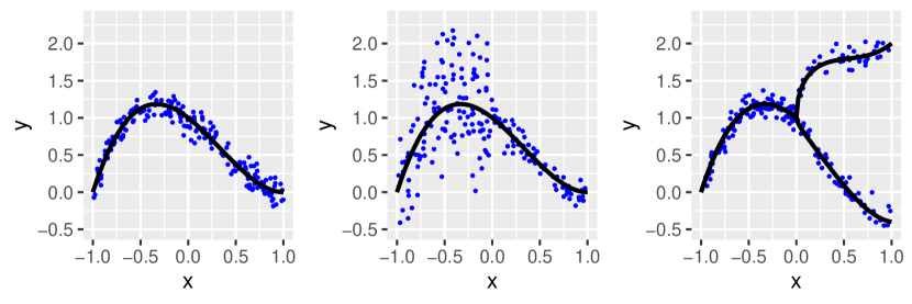
Figure 5: Illustration of the settings considered for $\mathcal{M}={\mathbb{R}}$: Setting 1 (nonlinear regression with homoscedastic variability, left panel); Setting 2 (nonlinear regression with heteroscedastic variability, middle panel); Setting 3 (nonlinear regression with bimodal pattern, right panel). Blue points are the observed data for the training set; the black curves are the underlying regression functions or the mixture regression function (in the right panel).

We first check the influence of bandwidth choice on marginal coverage level and average length of the prediction sets. We considered sample sizes $n=500,1000,2000$ and 200 Monte Carlo runs for each setting. Conditional coverage was evaluated on a test set with a sample size of 2000 with the same distribution as the training set for each setting. Marginal coverage levels and lengths of prediction sets for Setting 1 (Nonlinear regression with homoscedastic variability) are shown in Figure 6 and for Setting 2 (Nonlinear regression with heteroscedastic variability) and Setting 3 (Nonlinear regression with a bimodal pattern) in Supplement S5. One key feature of conformal inference is that the choice of conformity scores does not affect the coverage level but does affect the size (length) of the prediction sets. This is verified in Figure 6. Due to the bias and variance trade-off for the local linear smoother, the length of the prediction set as a function of the bandwidth is convex. As the sample size increases, the lengths of the conformal sets and the optimal bandwidths decrease, consistent with theory.

Next we check conditional coverage levels and lengths of the conformal prediction sets for both conditional profile scores and the HPD-split scores proposed in Izbicki et al. (2022). The latter is implemented using R code available at https://github.com/rizbicki/predictionBands, using the default settings. As illustrated in the first row of Figure 7, the proposed method consistently achieves conditional coverage across all settings. In Setting 2 (nonlinear regression with heteroscedastic variability) and Setting 3 (nonlinear regression with a bimodal pattern), where there is a change point in mean and variance at $x=0$, the HPD-split shows varying coverage levels for $x\in(-1,0)$ and $x\in(0,1)$, only achieving marginal coverage. In contrast, conditional profile scores generally achieve conditional validity for all three settings. The spike at $x=0$ is caused by the change points and kernel smoothing. Moreover, the second row of Figure 7 reveals that the proposed method results in prediction sets with shorter lengths compared to the HPD-split in all three settings, demonstrating the efficiency of conditional profile scores.

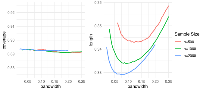
Figure 6: Average marginal coverage levels (left panel) and lengths of prediction sets (right panel) over 200 Monte Carlo runs for varying bandwidths $h$ for Setting 1 (nonlinear regression with homoscedastic variability). The target coverage level is $90\%$.

Next we consider responses in metric spaces, specifically responses on the unit sphere $\mathbb{S}^{2}:=\{p\in\mathbb{R}^{3}|p^{\top}p=1\}$ and in the 2-Wasserstein space. Note that $\mathbb{S}^{2}$ is a 2-dimensional Riemannian manifold endowed with the geodesic distance $d(p,q)=\arccos(p^{\top}q)$. The tangent space at a point $p$ is $T_{p}:=\{y\in\mathbb{R}^{3}|y^{\top}p=0\}$. For all $p\in\mathbb{S}^{2}$ and $v\in T_{p}$, the Riemannian exponential map that projects $v$ onto $\mathbb{S}^{2}$ is defined by

$$\exp_{p}v=\cos(\|v\|)p+\sin(\|v\|)\|v\|^{-1}v.$$

• Setting 4 (Responses in the unit sphere $\mathbb{S}^{2}$). The responses are generated by

  $$y_{i}=\exp_{\mu(x_{i})}V_{i}(x_{i}),$$

  with $\mu(x)=(\sin(\pi x/2),\cos(\pi x/2),0)^{\top}$ and $V_{i}=(0,0,\epsilon_{i})^{\top}$, where $\epsilon_{i}$ are random samples from $\mathcal{N}(0,0.5^{2})$.

For the next setting with distributional data in the 2-Wasserstein space, we adopt addition and scalar multiplication operations in the transport space $\mathbb{T}:=\{T:[0,1]\mapsto[0,1],\ T(0)=0,\ T(1)=1,\ T\text{ is increasing}\}$ following Zhu and Müller (2023), as follows,

• Addition: $T_{1}\oplus T_{2}=T_{2}\circ T_{1}$ for $T_{1},T_{2}\in\mathbb{T}$.

• Scalar multiplication: for any $|\alpha|\leq 1$ and $T\in\mathbb{T}$,

  $$\alpha\odot T(x):=\,\begin{cases}x+\alpha(T(x)-x),&0<\alpha\leq 1,\\ x,&\alpha=0,\\ x+\alpha\left(x-T^{-1}(x)\right),&-1\leq\alpha<0.\end{cases}$$

For distributions defined on $(0,1)$ that are absolutely continuous with respect to the Lebesgue measure, their corresponding quantile functions can be regarded as elements of $\mathbb{T}$. For the 2-Wasserstein space, we represent the random elements in $\mathcal{W}_{2}$ through their quantile functions.

• Setting 5 (Distributional responses in the Wasserstein space $\mathcal{W}_{2}$). The responses are $y_{i}=\operatorname{Trun}\mathcal{N}(f(x_{i}),0.5)\oplus\epsilon_{i}$, where $\operatorname{Trun}\mathcal{N}$ is the truncated normal distribution on $(0,1)$, $f(x_{i})=0.8(x_{i}-1)^{2}(x_{i}+1)$, and the $\epsilon_{i}$ are random distributions drawn from
  $\operatorname{Unif}[-0.5,0.5]\odot\mathrm{Beta}(2,2)$.

The conditional validity of the proposed conditional profile scores for Setting 4 and Setting 5 is demonstrated in Figure 8. Additional simulation results, such as marginal coverage levels and sizes of the prediction sets can be found in Supplement S5.

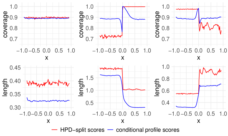
Figure 7: Average conditional coverage (first row) and prediction set length (second row) over 200 Monte Carlo runs in dependence on the level of the predictor $x$. The same three settings for $\mathcal{M}={\mathbb{R}}$ as in Figure 5 are considered for sample size $n=2000$ and target coverage level 90%. The prediction sets are obtained by Algorithm 1; blue lines represent results for conditional profile scores and red lines for the HPD-split scores in Izbicki et al. (2022).

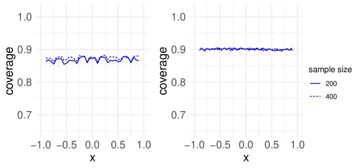
Figure 8: Average conditional coverage levels over 200 Monte Carlo runs for a target coverage level at $90\%$ for Setting 4 (left panel) and Setting 5 (right panel).

6.2 Multivariate predictors

In this subsection, we show the performance of the proposed method described in Section 5 for multivariate predictors and scalar responses. In addition to evaluating the conditional coverage and size of the prediction set, we also examine the mean square error of the slope parameter in the single index Fréchet regression,

$$\operatorname{MSE}(\bm{\theta_{0}},\hat{\bm{\theta}})=\|\hat{\bm{\theta}}-\bm{\theta_{0}}\|^{2}.$$ (27)

For responses we considered the same scenarios as for univariate responses and again compared the proposed conditional profile scores with HPD-split scores (Izbicki et al., 2022) for Euclidean responses across three different settings, as well as for responses located on the unit sphere as well as distributional responses.

• Setting 6 (Multivariate predictor with homoscedastic variability): The predictors are $\bm{X}_{i}=(x_{i1},x_{i2})^{\top}$ with $x_{ik}$ independently and identically distributed $\sim\mathrm{Unif}(-1,1)$ and $\bm{\theta_{0}}=(1,0)^{\top}$. The responses are generated by $y_{i}=f(\bm{X}_{i}^{\top}\bm{\theta_{0}})+\epsilon_{i}$ with $f(x)=(x-1)^{2}(x+1)$ and the $\epsilon_{i}$ are random samples from $\mathcal{N}(0,0.1^{2})$.

• Setting 7 (Multivariate predictor with heteroscedastic variability): The predictors are $\bm{X}_{i}=(x_{i1},x_{i2})^{\top}$ with $x_{ik}$ $\sim\mathrm{Unif}(-1,1)$ and $\bm{\theta_{0}}=(1,0)^{\top}$. The responses are generated by $y_{i}=f(\bm{X}_{i}^{\top}\bm{\theta_{0}})+\epsilon_{i}(\bm{X}_{i}^{\top}\bm{\theta_{0}})$ with $f(x)=(x-1)^{2}(x+1)$ and the $\epsilon_{i}(x)$ are random samples from $\mathds{1}_{-1\leq x\leq 0}\mathcal{N}(0,0.5^{2})+\mathds{1}_{0<x\leq 1}\mathcal{N}(0,0.1^{2})$.

• Setting 8 (Multivariate predictor with a bimodal pattern): The predictors are $\bm{X}_{i}=(x_{i1},x_{i2})^{\top}$ with $x_{ik}$ $i.i.d.$ $\sim\mathrm{Unif}(-1,1)$ and $\bm{\theta_{0}}=(1,0)^{\top}$, and responses are

  $$y_{i}\sim 0.5\mathcal{N}\left(f(\bm{X}_{i}^{\top}\bm{\theta_{0}})+g(\bm{X}_{i}^{\top}\bm{\theta_{0}}),0.1^{2}\right)+0.5\mathcal{N}\left(f(\bm{X}_{i}^{\top}\bm{\theta_{0}})-0.2g(\bm{X}_{i}^{\top}\bm{\theta_{0}}),0.1^{2}\right),$$

  where $f(x)=(x-1)^{2}(x+1)$ and $g(x)=2\sqrt{x}\mathds{1}_{\{x\geq 0\}}$.

Figure 9 demonstrates conditional coverages and lengths of prediction sets, in analogy to Figure 7. Conditional profiles scores outperform HPD-split scores in both coverage and size. For responses on the unit sphere with a multivariate predictor, we consider the following setting. Figure S.8 in Supplement S5 demonstrates that the proposed Fréchet single index approach with Algorithm 1 achieves conditional validity for this setting (Setting 9).

• Setting 9 (Multivariate predictor with responses in $\mathbb{S}^{2}$): The predictors are

  $$\bm{X}_{i}=(x_{i1},x_{i2},x_{i3},x_{i4})^{\top}$$

  with $x_{ik}$ independently and identically distributed $\sim\mathrm{Unif}(-1,1)$ and $\bm{\theta_{0}}=(1,0,0,0)^{\top}$. The responses are generated by $y_{i}=\exp_{\mu(\bm{x_{i}}^{\top}\bm{\theta_{0}})}V_{i}(x_{i})$, where

  $$\mu(x)=(\sin(\pi x/2),\cos(\pi x/2),0)^{\top}$$

  and $V_{i}=(0,0,\epsilon_{i})^{\top}$ where the $\epsilon_{i}$ are random samples from $\mathcal{N}(0,0.5^{2})$.

We also obtained $\operatorname{MSE}(\hat{\bm{\theta}},\bm{\theta_{0}})$ as defined in (27) for Settings 6-9 across various sample sizes. The results in Table 1 indicate that $\operatorname{MSE}(\hat{\bm{\theta}},\bm{\theta_{0}})$ decreases as the sample size increases across all settings.

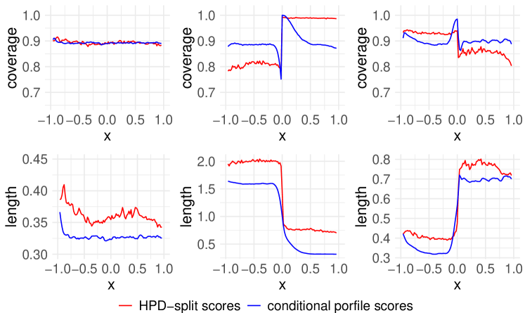
Figure 9: Average conditional coverages (first row) and prediction set lengths (second row) over 200 Monte Carlo runs in dependence on the single index level $x$ for multivariate predictors in Settings 6-8 for sample size $n=2000$ and target coverage level 90%. The prediction sets are obtained by Algorithm 1 as in (24) – (26); blue lines represent the proposed conditional profile scores, and red lines the HPD-split scores in Izbicki et al. (2022).

Table 1: Average $\operatorname{MSE}(\hat{\bm{\theta}},\bm{\theta_{0}})$ for the estimated single index parameter $\hat{\bm{\theta}}$ over 200 Monte Carlo runs for various settings, with standard deviations in parentheses, where all values are multiplied by $10^{2}$ for better visualization.

	$\mathcal{M}={\mathbb{R}}$				$\mathcal{M}=\mathbb{S}^{2}$
$n$	Setting 6	Setting 7	Setting 8		$n$	Setting 9
500	0.52(0.45)	2.85(2.71)	20.23(32.50)		200	12.84(43.21)
1000	0.38(0.30)	1.82(1.86)	8.05(21.35)		500	7.58(34.01)
2000	0.24(0.23)	1.22(1.14)	2.42(2.48)

7 Data illustrations

7.1 New York taxi data

Trip records for yellow taxis in New York City, with times and locations for pick-ups and drop-offs, can be accessed via https://www.nyc.gov/site/tlc/about/tlc-trip-record-data.page. We focus on the pick-up and drop-off points located within Manhattan. Omitting Governor’s Island, Ellis Island and Liberty Island, we divide the remaining 66 zones of Manhattan into 13 distinct regions. The predictor $x$ records the time of day, ranging from 4 AM to 8 PM and the response is a network representing the number of customers commuting between the selected areas by taking a yellow taxi at time $x$; we include all $N=260$ weekdays within the year 2023. For each weekday $i$, there are $n_{i}$ records collected from 4 AM to 8 PM. We divide the time domain $(4,20)$ (from 4 AM to 8 PM) into bins $S_{i1}=(a_{i0},a_{i1}),S_{i2}=(a_{i1},a_{i2}),\ldots,S_{B_{i}}=(a_{i(B_{i}-1)},a_{iB_{i}})$, ensuring there are $N=1000$ records within each bin, with $4=a_{i0}<a_{i1}<a_{i2}<\cdots<a_{i(B_{i}-1)}<a_{iB_{i}}=20$ and $B_{i}=\lfloor n_{i}/N\rfloor$. For each bin $S_{k}$, $k=1,\ldots,B_{i}$, we pool all records whose pickup times fall within this bin to construct the 13 by 13 adjacency matrix $y_{ik}$, which represents the response at time $x_{ik}=(a_{i(k-1)}+a_{ik})/2$. Each adjacency matrix’s edge weights are normalized against its maximum edge weight, ensuring they range between $[0,1]$. The resulting pairs $\{(x_{ik},y_{ik})\}_{k=1}^{B_{i}}$ from all weekdays are pooled together to form the final dataset.

We use the Frobenius metric $d_{F}$ as the metric between graph adjacency matrices,

$$d_{F}(\mathbf{A},\mathbf{B})=\sqrt{\operatorname{tr}\left[(\mathbf{A}-\mathbf{B})(\mathbf{A}-\mathbf{B})^{\top}\right]},$$

for $\mathbf{A},\mathbf{B}\in\mathbb{R}^{13\times 13}$. The data are divided into training, calibration, and testing sets in a 4:4:2 proportion. We implemented Algorithm 1 and evaluated the conditional coverage on the testing set. Figure 10 indicates that the proposed conditional profile score ensures conditional coverage across all $x$ in the time range. We also examined the conditional coverage for holidays and weekends in 2023, but still using training and calibration data collected for weekdays in Algorithm 1. Figure 10 reveals that the conditional coverages for holidays significantly deviate from the target, confirming that taxi transportation patterns on weekdays and non-weekdays do not align.

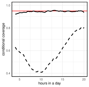
Figure 10: Conditional coverage levels for taxi data. The target coverage level is 95%, as indicated by the red solid line. The conditional coverage levels evaluated on the testing set (black solid line) derived from weekdays differs substantially from the conditional coverage levels evaluated using data from weekends and holidays (dashed line).

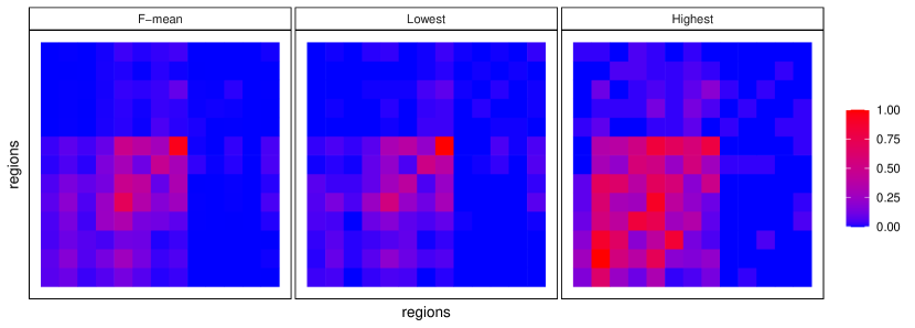
Figure 11: Heat maps for networks represented by graph adjacency matrices at time 3 PM from the training set of weekday data. The Fréchet mean is in the left panel, the network with the lowest conditional profile score in the middle panel and the network with the highest conditional profile score in the right panel.

Figure 11 displays heatmaps for the Fréchet mean and for networks with the lowest and highest conditional profile scores from the training set. The heatmap for the network with the lowest score has a pattern similar to the Fréchet mean, indicating its corresponding adjacency matrix is at the center of the dataset. The heatmap for the network with the highest score presents a very different pattern from the previous two, indicating that it sits near the boundary of the prediction set and has a higher likelihood of being an outlier.

7.2 U.S. energy data

The global energy landscape has undergone profound changes over the last thirty years, driven by technological innovations, economic shifts, and evolving societal needs. Data on the sources of energy used for electricity generation across the U.S. are available at https://www.eia.gov/electricity/data/state/. As an illustration of the proposed method, we considered three categories of energy sources and their corresponding proportions: I. Coal, Petroleum, Wood, and Wood Derived Fuels; II. Natural Gas; III. Hydroelectric, Wind, Nuclear, Geothermal, Solar Thermal and Photovoltaic. Sources in category I are traditional energy sources known to emit high levels of greenhouse gases and have historically been associated with severe air pollution. Sources in category II are a cleaner alternatives and their contribution has steadily grown. Sources in category III represent renewable energy and other eco-friendly sources.

The predictors $x$ are calendar years ranging from 1990 to 2021. The corresponding responses are defined as $y(x)=(U^{1/2}(x),V^{1/2}(x),W^{1/2}(x))$, where $U(x)$, $V(x)$, and $W(x)$ denote the proportions of energy sources I, II, and III used for electricity generation in the given year $x$. These proportions constitute compositional data as they satisfy the condition $U(x)+V(x)+W(x)=1$ for every calendar year $x$. Figure 12 shows a clear trend in the prediction set obtained by the proposed method, moving from the bottom left to the top right as the years progress. This indicates a decreasing dependence on traditional fossil fuels and an increasing share of natural gas and renewable energy sources.

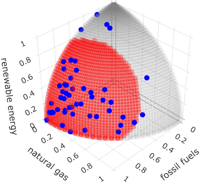
1990

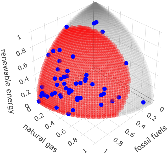
1996

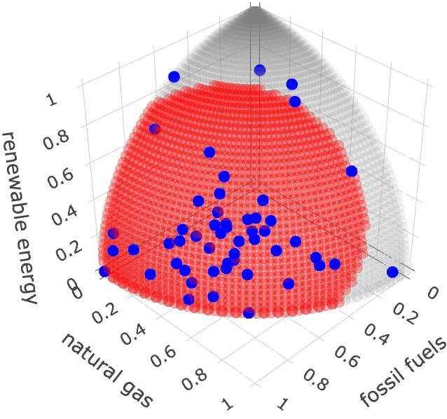
2002

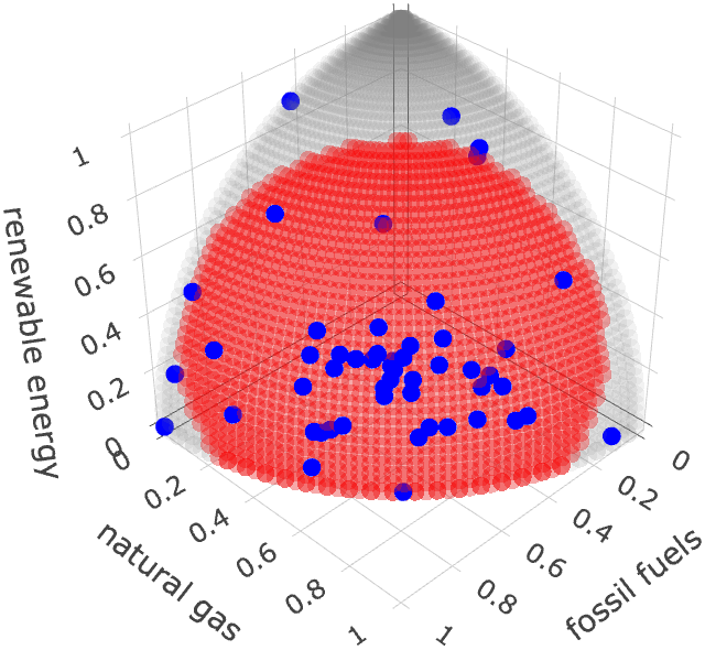
2008

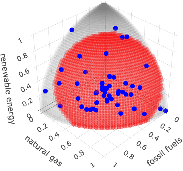
2014

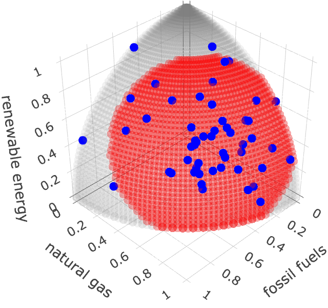
2021

Figure 12: Illustration of energy data sources and corresponding conformal sets for calendar years 1990, 1996, 2002, 2008, 2014, and 2021. The the front-right axis represents the proportion of fossil fuels (sources I), front-left axis represents the proportion of natural gas (sources II), and the rear axis represents the proportion of renewable energy (sources III). Blue points represent the square root of proportions of energy sources for each state. The red areas are the conformal prediction sets obtained with the proposed conditional profile score.

8 Discussion

We extend the distance profiles proposed by Dubey et al. (2024) to a conditional version and propose the profile average transport costs as a measure of the centrality of any element in a metric space with respect to the underlying conditional distribution of $Y|X$. There are major distinctions between the proposed profile average transport costs and the transport ranks introduced in Dubey et al. (2024). While transport ranks account for the directionality of optimal transports, profile average transport costs focus solely on the costs of transport between two distance profiles and ignore the direction of the transport. Consequently, while transport ranks identify the most centrally located element globally, the proposed CPCs can capture local modes with respect to the underlying conditional distributions, aiding in the construction of conformal prediction sets.

The key for successful conformal inference lies in the choice of a good conformity score. In general metric spaces, residual scores $\hat{R}(x,y)=d(\hat{f}(x),y)$ may seem to be the most straightforward approach, however for complex object data these have many shortcomings. First, such residual scores can only achieve marginal coverage, and the size of the resulting prediction sets is the same for all predictor levels. This results in poor prediction sets when there is heteroscedasticity or other distributional change in $Y$ when predictors vary. Moreover, residual scores depend crucially on the regression function estimator $\hat{f}$. In many situations, including when the conditional distribution of $Y|X$ is bimodal or multimodal, estimates $\hat{f}$ will not perform well. The proposed conditional profile scores are determined solely by the distances within the metric space, leading to an intrinsic approach that does not require projections of the data into extrinsic spaces. This distance-based approach simplifies computations, as it can be readily applied for any metric space without the need for transformations or manipulations of the data structure. The effectiveness of the proposed method is demonstrated through comparison with the HPD-split approach (Izbicki et al., 2022) for Euclidean responses. The proposed method outperforms the HPD-split in terms of both better conditional coverage accuracy and shorter prediction set lengths even for traditional data types.

While this paper primarily focuses on obtaining prediction sets within the conformal framework, an additional benefit of the proposed profile average transport costs is their ability to act as substitutes for density functions within general metric spaces. Numerous methodologies in Euclidean spaces rely on density functions for a variety of applications, including hypothesis testing, clustering, classification, and outlier detection. The profile average transport cost approach paves the way for adapting such approaches and further developing such methods will be a promising topic for future research.

References

- Ambrosio et al. (2008) Ambrosio, L., N. Gigli, and G. Savaré (2008). Gradient Flows: in Metric Spaces and in the Space of Probability Measures. Springer Science & Business Media.
- Angelopoulos et al. (2024) Angelopoulos, A., E. Candès, and R. J. Tibshirani (2024). Conformal pid control for time series prediction. In Adv. Neural Inf. Process. Syst. 2024, Volume 36.
- Barber et al. (2023) Barber, R. F., E. J. Candès, A. Ramdas, and R. J. Tibshirani (2023). Conformal prediction beyond exchangeability. Ann. Stat. 51(2), 816–845.
- Bates et al. (2023) Bates, S., E. Candès, L. Lei, Y. Romano, and M. Sesia (2023). Testing for outliers with conformal p-values. Ann. Stat. 51(1), 149–178.
- Bhattacharjee and Müller (2023) Bhattacharjee, S. and H.-G. Müller (2023). Single index fréchet regression. Ann. Stat. 51(4), 1770–1798.
- Bigot et al. (2017) Bigot, J., R. Gouet, T. Klein, and A. López (2017). Geodesic PCA in the Wasserstein space by convex PCA. Ann. inst. Henri Poincare (B) Probab. Stat. 53, 1–26.
- Billera et al. (2001) Billera, L. J., S. P. Holmes, and K. Vogtmann (2001). Geometry of the space of phylogenetic trees. Adv. Appl. Math. 27(4), 733–767.
- Candès et al. (2023) Candès, E., L. Lei, and Z. Ren (2023). Conformalized survival analysis. J. R. Stat. Soc. Ser. B Stat. Methodol. 85(1), 24–45.
- Chang (1989) Chang, T. (1989). Spherical regression with errors in variables. Ann. Stat. 17(1), 293–306.
- Chen et al. (2011) Chen, D., P. Hall, and H.-G. Müller (2011). Single and multiple index functional regression models with nonparametric link. Ann. Stat. 39(3), 1720 – 1747.
- Chen and Müller (2012) Chen, D. and H.-G. Müller (2012). Nonlinear manifold representations for functional data. Ann. Stat. 40(1), 1 – 29.
- Chen et al. (2023) Chen, Y., Z. Lin, and H.-G. Müller (2023). Wasserstein regression. J. Amer. Statist. Assoc. 118(542), 869–882.
- Chernozhukov et al. (2021) Chernozhukov, V., K. Wüthrich, and Y. Zhu (2021). Distributional conformal prediction. Proc. Natl. Acad. Sci. U. S. A. 118(48), e2107794118.
- Choi and Hall (1998) Choi, E. and P. Hall (1998). On bias reduction in local linear smoothing. Biometrika 85(2), 333–345.
- Cornea et al. (2017) Cornea, E., H. Zhu, P. Kim, and J. G. Ibrahim (2017). Regression models on riemannian symmetric spaces. J. R. Stat. Soc. Ser. B Stat. Methodol. 79(2), 463–482.
- Dryden et al. (2009) Dryden, I. L., A. Koloydenko, and D. Zhou (2009). Non-Euclidean statistics for covariance matrices, with applications to diffusion tensor imaging. Ann. Appl. Stat. 3(3), 1102 – 1123.
- Du et al. (2023) Du, L., X. Guo, W. Sun, and C. Zou (2023). False discovery rate control under general dependence by symmetrized data aggregation. J. Amer. Statist. Assoc. 118(541), 607–621.
- Dubey et al. (2024) Dubey, P., Y. Chen, and H.-G. Müller (2024). Metric statistics: exploration and inference for random objects with distance profiles. arXiv preprint arXiv:2202.06117.
- Dubey and Müller (2020) Dubey, P. and H.-G. Müller (2020). Functional models for time-varying random objects. J. R. Stat. Soc. Ser. B Stat. Methodol. 82(2), 275–327.
- Fan (1993) Fan, J. (1993). Local linear regression smoothers and their minimax efficiencies. Ann. Stat. 21(1), 196–216.
- Fan and Gijbels (1992) Fan, J. and I. Gijbels (1992). Variable bandwidth and local linear regression smoothers. Ann. Stat. 20(4), 2008–2036.
- Ferraty et al. (2011) Ferraty, F., J. Park, and P. Vieu (2011). Estimation of a functional single index model. In Recent Advances in Functional Data Analysis and Related Topics, pp. 111–116. Springer.
- Fisher et al. (1993) Fisher, N. I., T. Lewis, and B. J. Embleton (1993). Statistical Analysis of Spherical Data. Cambridge University Press.
- Fletcher (2013) Fletcher, T. P. (2013). Geodesic regression and the theory of least squares on riemannian manifolds. Int. J. Comput. Vis. 105, 171–185.
- Foygel Barber et al. (2021) Foygel Barber, R., E. J. Candès, A. Ramdas, and R. J. Tibshirani (2021). The limits of distribution-free conditional predictive inference. Information and Inference: A Journal of the IMA 10(2), 455–482.
- Gao and Wellner (2009) Gao, F. and J. A. Wellner (2009). On the rate of convergence of the maximum likelihood estimator of ak-monotone density. Sci. China Math. 52(7), 1525–1538.
- Gibbs and Candès (2021) Gibbs, I. and E. Candès (2021). Adaptive conformal inference under distribution shift. In Adv. Neural Inf. Process. Syst. 2021, pp. 1660–1672.
- Gibbs and Candès (2022) Gibbs, I. and E. Candès (2022). Conformal inference for online prediction with arbitrary distribution shifts. arXiv preprint arXiv:2208.08401.
- Hall (1989) Hall, P. (1989). On projection pursuit regression. Ann. Stat. 17(2), 573–588.
- Hall and Marron (1997) Hall, P. and J. S. Marron (1997). On the role of the shrinkage parameter in local linear smoothing. Probab. Theory Relat. Fields 108, 495–516.
- Hall et al. (1999) Hall, P., R. C. Wolff, and Q. Yao (1999). Methods for estimating a conditional distribution function. J. Amer. Statist. Assoc. 94(445), 154–163.
- Hu and Lei (2023) Hu, X. and J. Lei (2023). A two-sample conditional distribution test using conformal prediction and weighted rank sum. J. Amer. Statist. Assoc., 1–19.
- Ichimura (1993) Ichimura, H. (1993). Semiparametric least squares (sls) and weighted sls estimation of single-index models. J. Econom. 58(1-2), 71–120.
- Izbicki et al. (2022) Izbicki, R., G. Shimizu, and R. B. Stern (2022). Cd-split and hpd-split. J. Mach. Learn. Res. 23, 1–32.
- Jeon and Park (2020) Jeon, J. M. and B. U. Park (2020). Additive regression with Hilbertian responses. Ann. Stat. 48(5), 2671 – 2697.
- Jiang and Wang (2011) Jiang, C.-R. and J.-L. Wang (2011). Functional single index models for longitudinal data. Ann. Stat. 39(1), 362 – 388.
- Kim et al. (2020) Kim, J., N. A. Rosenberg, and J. A. Palacios (2020). Distance metrics for ranked evolutionary trees. Proc. Natl. Acad. Sci. U.S.A. 117(46), 28876–28886.
- Kuchibhotla and Patra (2020) Kuchibhotla, A. K. and R. K. Patra (2020). Efficient estimation in single index models through smoothing splines. Bernoulli 26(2), 1587–1618.
- Lei et al. (2018) Lei, J., M. G’Sell, A. Rinaldo, R. J. Tibshirani, and L. Wasserman (2018). Distribution-free predictive inference for regression. J. Amer. Statist. Assoc. 113(523), 1094–1111.
- Lei et al. (2013) Lei, J., J. Robins, and L. Wasserman (2013). Distribution-free prediction sets. J. Amer. Statist. Assoc. 108(501), 278–287.
- Lei and Wasserman (2014) Lei, J. and L. Wasserman (2014). Distribution-free prediction bands for non-parametric regression. J. R. Stat. Soc. Ser. B Stat. Methodol. 76(1), 71–96.
- Lin and Müller (2021) Lin, Z. and H.-G. Müller (2021). Total variation regularized fréchet regression for metric-space valued data. Ann. Stat. 49(6), 3510–3533.
- Meinshausen et al. (2009) Meinshausen, N., L. Meier, and P. Bühlmann (2009). P-values for high-dimensional regression. J. Amer. Statist. Assoc. 104(488), 1671–1681.
- Petersen and Müller (2016) Petersen, A. and H.-G. Müller (2016). Functional data analysis for density functions by transformation to a hilbert space. Ann. Stat. 44(1), 183–218.
- Petersen and Müller (2019) Petersen, A. and H.-G. Müller (2019). Fréchet regression for random objects with euclidean predictors. Ann. Stat. 47(2), 691–719.
- Petersen et al. (2022) Petersen, A., C. Zhang, and P. Kokoszka (2022). Modeling probability density functions as data objects. Econometrics and Statistics 21, 159–178.
- Thanwerdas and Pennec (2023) Thanwerdas, Y. and X. Pennec (2023). O(n)-invariant riemannian metrics on spd matrices. Linear Algebra Appl. 661, 163–201.
- Villani et al. (2009) Villani, C. et al. (2009). Optimal Transport: Old and New. Springer.
- Vovk (2012) Vovk, V. (2012). Conditional validity of inductive conformal predictors. In Asian Conference on Machine Learning, pp. 475–490.
- Vovk (2021) Vovk, V. (2021, 08–10 Sep). Conformal testing in a binary model situation. In Proceedings of the Tenth Symposium on Conformal and Probabilistic Prediction and Applications, Volume 152 of Proc. Mach. Learn. Res., pp. 131–150.
- Vovk et al. (2005) Vovk, V., A. Gammerman, and G. Shafer (2005). Algorithmic Learning in a Random World, Volume 29. Springer.
- Vovk et al. (2009) Vovk, V., I. Nouretdinov, and A. Gammerman (2009). On-line predictive linear regression. Ann. Stat., 1566–1590.
- Vovk et al. (2021) Vovk, V., I. Petej, I. Nouretdinov, E. Ahlberg, L. Carlsson, and A. Gammerman (2021). Retrain or not retrain: Conformal test martingales for change-point detection. In Conformal and Probabilistic Prediction and Applications, pp. 191–210.
- Wang et al. (2023) Wang, X., J. Zhu, W. Pan, J. Zhu, and H. Zhang (2023). Nonparametric statistical inference via metric distribution function in metric spaces. Journal of the American Statistical Association. (to appear).
- Wasserman and Roeder (2009) Wasserman, L. and K. Roeder (2009). High dimensional variable selection. Ann. Stat. 37(5A), 2178–2201.
- Yang et al. (2024) Yang, Z., E. Candès, and L. Lei (2024). Bellman conformal inference: calibrating prediction intervals for time series. arXiv preprint arXiv:2402.05203.
- Yuan et al. (2012) Yuan, Y., H. Zhu, W. Lin, and J. S. Marron (2012). Local polynomial regression for symmetric positive definite matrices. J. R. Stat. Soc. Ser. B Stat. Methodol. 74(4), 697–719.
- Zhou et al. (2023) Zhou, H., F. Yao, and H. Zhang (2023). Functional linear regression for discretely observed data: from ideal to reality. Biometrika 110(2), 381–393.
- Zhou and He (2008) Zhou, J. and X. He (2008). Dimension reduction based on constrained canonical correlation and variable filtering. Ann. Stat. 36(4), 1649 – 1668.
- Zhu and Müller (2023) Zhu, C. and H.-G. Müller (2023). Autoregressive optimal transport models. J. R. Stat. Soc. Ser. B Stat. Methodol. 85(3), 1012–1033.
- Zhu and Zhu (2009) Zhu, L.-P. and L.-X. Zhu (2009). On distribution-weighted partial least squares with diverging number of highly correlated predictors. J. R. Stat. Soc. Ser. B Stat. Methodol. 71(2), 525–548.
- Zou et al. (2020) Zou, C., G. Wang, and R. Li (2020). Consistent selection of the number of change-points via sample-splitting. Ann. Stat. 48(1), 413.