Phase shifts, band geometry and responses in triple-Q charge and spin density waves

Abstract

Recently, there has been growing interest in the impacts of phase shifts within the triple-Q spin density wave (SDW) order parameters. Concurrently, it is widely recognized that incommensurate triple-Q charge density waves (CDW) are also prevalent in low-dimensional materials, where the phase degrees of freedom in the order parameters are generally allowed. In this study, we systematically investigate the pivotal effects arising from both triple-Q CDW and SDW order parameters, with particular consideration given to possible phase shifts. We show that the phase shifts play a crucial role in determining the real-space topology of triple-Q density waves. More importantly, we show that the triple-Q CDW and SDW order parameters would influence the band geometry in the momentum space, where multiband Dirac-like fermions are induced by the triple-Q density wave order parameters near the Fermi energy. Furthermore, we explicitly establish that such nontrivial band geometry, combined with symmetry-breaking induced by phase shifts, leads to a variety of intriguing linear and nonlinear responses.

Introduction.— For the incommensurate density waves, there exhibits possible phase shifts that can be continuously changed without affecting the energy. As a result, the incommensurate density waves exhibit an exotic gapless collective excitation — phason. In the presence of impurities, phasons are pinned and become effectively gapped. But these phasons can be excited with an electric field beyond the threshold, leading to the so-called depinning phenomena. Such phenomena have been observed in both charge density wave (CDW) and spin density wave (SDW) systems [1, 2, 3, 4, 5, 6, 7]. Moreover, the CDWs and SDWs often share similar physics with each other. For example, the sliding dynamics of CDWs and SDWs in the flow region are unified with the same theoretical framework recently [8], while Galilean relativity physics has also been discussed in both moving CDW [9] and moving SDW systems [10]. It is generally interesting and profound in identifying the common physics shared by various density wave systems.

The phase shifts are naturally expected to appear in multi-Q incommensurate density waves as well. Especially, the incommensurate triple-Q CDW systems are widely recognized in low-dimensional materials, such as layered transition-metal dichalcogenides 1T TaS₂, 1T TiSe₂, 2H TaSe₂ [11], while triple-Q SDWs are commonly found in noncolinear magnetic materials, such as skymrion crystals (SkX) [12, 13, 14, 15]. Moreover, the important effects of phase shifts on the SkX were recently highlighted [16, 17, 18], which play a crucial role in affecting the scalar spin chirality and lowering the rotational symmetry in SkX [17]. However, a theoretical work that simultaneously describes the effects of phase shifts in both incommensurate triple-Q CDW and SDW systems is still lacking.

In this work, we present a minimal theory to capture the phase shifts, band geometry, and their interplay on various responses in two-dimensional triple-Q density wave systems. The theoretical framework is applied to both triple-Q CDWs and SDWs in the same way, i.e., being treated on equal footing. We first provide a symmetry classification of possible triple-Q density waves according to the $C_{3}$ point group, which would naturally generate the triple-Q spiral spin textures as well as the triple-Q CDW order. Next, we display the real-space landscape and topology of triple-Q density waves. Importantly, by tuning the phase shifts continuously, we show that the meron-antimeron crystals are the transition boundaries where the quantized skyrmion charge flips sign. Then, we demonstrate that even with the most trivial single quadratic band dispersion, the triple-Q density waves would be able to influence its band geometry by creating multiband Dirac-like fermions near the Fermi energy. Finally, we explicitly show that the nontrivial band geometry together with possible inversion or rotational symmetry breaking induced by the phase shift would enable rich linear and nonlinear responses in the incommensurate triple-Q CDW and triple-Q SDW systems.

Symmetry classifications of triple-Q density waves.— Let us first present the form of triple-Q density waves in two dimensions from the symmetry point of view. Without loss of generality, the three Q vectors are defined as $\bm{Q}_{1}=(1,0)Q,\bm{Q}_{2}=(-\frac{1}{2},\frac{\sqrt{3}}{2})Q,\bm{Q}_{3}=(-\frac{1}{2},-\frac{\sqrt{3}}{2})Q$, where the angle with respect to each other are $120$ ^∘. The phase shifts along $\bm{Q}_{\nu}$ direction are defined as $\theta_{\nu}$. The structure of CDW/SDW is then determined by $\Theta=\frac{1}{\sqrt{3}}(\theta_{1}+\theta_{2}+\theta_{3})$, while the translational motion of CDW/SDW are determined by $\theta_{X}=\frac{1}{\sqrt{6}}(2\theta_{1}-\theta_{2}-\theta_{3})$, $\theta_{Y}=\frac{1}{\sqrt{2}}(\theta_{2}-\theta_{3})$ [19, 20], i.e. phasons. In this work, to preserve $C_{3z}$ symmetry, we would set $\theta_{1}=\theta_{2}=\theta_{3}$. But the coupling to the two phasons given by $\theta_{X}$ and $\theta_{Y}$ is an interesting problem for future study. As shown in Table I, we can classify triple-Q density waves using the irreducible representations of the $C_{3}$ point group, where the spin Pauli matrices are defined as $\sigma_{j}$, the phase shift is defined as $\theta$, and the position vector is $\bm{r}$.

Table 1: Classifications of triple-Q density waves using the irreducible representations of the $C_{3z}$ point group. Here, $\omega=e^{i2\pi/3}$, $\bm{Q}_{1}=(1,0)Q,\bm{Q}_{2}=(-\frac{1}{2},\frac{\sqrt{3}}{2})Q,\bm{Q}_{3}=(-\frac{1}{2},-\frac{\sqrt{3}}{2})Q$, $\sigma_{j}$ are spin Pauli matrices.

$C_{3}$	basis functions	spin matrices
1	$f_{A}(\bm{r})=\sum_{\nu=1}^{3}\cos(\bm{Q}_{\nu}\cdot\bm{r}+\theta)$	$\sigma_{0},\sigma_{z}$
$\omega$	$f_{E_{1}}(\bm{r})=\sum_{\nu=1}^{3}\omega^{\nu-1}\sin(\bm{Q}_{\nu}\cdot\bm{r}+\theta)$	$\sigma_{+}=\sigma_{x}+i\sigma_{y}$
$\omega^{*}$	$f_{E_{2}}(\bm{r})=\sum_{\nu=1}^{3}\omega^{1-\nu}\sin(\bm{Q}_{\nu}\cdot\bm{r}+\theta)$	$\sigma_{-}=\sigma_{x}-i\sigma_{y}$

In the spinless case, the $C_{3z}$ invariant triple-Q density wave order parameter, i.e., CDW order parameter, is

$$\Delta_{\text{CDW}}(\bm{r})=2\Delta f_{A}(\bm{r})=2\Delta\sum_{\nu=1}^{3}\cos(\bm{Q}_{\nu}\cdot\bm{r}+\theta).$$ (1)

where $\Delta$ denotes the CDW potential, and $f_{A}(\bm{r})$ is the basis function of $A$ irreducible representation of $C_{3}$ point group. In the spinful case, the $C_{3z}$ invariant triple-Q density wave order parameter, i.e., SDW order parameter, is obtained as

$$\Delta_{\text{SDW}}(\bm{r})=\frac{\Delta}{2}[f_{E_{1}}(\bm{r})\sigma_{-}+f_{E_{2}}(\bm{r})\sigma_{+}]-\Delta f_{A}(\bm{r})\sigma_{z}.$$ (2)

Here, $f_{E_{1}}(\bm{r})$ and $f_{E_{2}}(\bm{r})$ (see Table I) are the basis functions of $E_{1}$ and $E_{2}$ irreducible representations of $C_{3}$ group. We can rewrite the form of $\Delta_{\text{SDW}}(\bm{r})$ as

$$\Delta_{\text{SDW}}(\bm{r})=\sum_{i}\bm{S}_{i}^{\text{spiral}}\cdot\bm{\sigma},$$ (3)

and obtain the triple-Q spiral spin textures [17]

$$\bm{S}_{i}^{\text{spiral}}=\Delta\sum_{\nu=1}^{3}(\sin\mathcal{Q}_{\nu}\cos\phi_{\nu},\sin\mathcal{Q}_{\nu}\sin\phi_{\nu},-\cos\mathcal{Q}_{\nu})$$ (4)

with $\mathcal{Q}_{\nu}=\bm{Q}_{\nu}\cdot\bm{r}_{i}+\theta$, $\phi_{\nu}=\frac{2\pi}{3}(\nu-1)$. Here, $\bm{Q}_{\nu}$ is the wave vector of $\nu$-th spiral.

For the sake of simplicity, we neglect the spin-orbit interaction in our model so that the direction of the spin-rotating plane does not matter. We shall also focus on the simplest case that the order parameter only exhibits the spatial and spin degree of freedom.

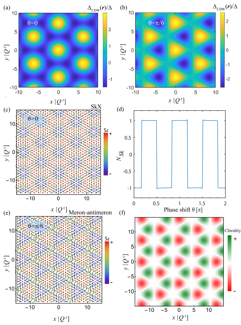
Figure 1: (a) and (b) The real-space dependence of triple-Q CDW potential $\Delta_{\text{CDW}}(\bm{r})$ at $\theta=0$ and $\theta=\pi/6$, respectively. (c) and (e) The triple-Q spiral spin textures at $\theta=0$ and $\theta=\frac{\pi}{6}$, respectively. (d) The total skyrmion charge $N_{sk}$ of each unit cell versus the phase shift $\theta$ calculated from the normalized spin vectors $\bm{s}$. (f) The real-space spin chirality $\chi=\bm{S}_{i}\cdot(\bm{S}_{j}\times\bm{S}_{k})$, where the site indcies $i,j,k$ are in counterclockwise order.

Real space landscape and topology of triple-Q density waves.— To visualize these order parameters and highlight the effects of the phase shift $\theta$ on the triple-Q density waves, we plot the real space landscape of triple-Q CDW and triple-Q SDW with various $\theta$ in Fig. 1.

Figs. 1(a) and (b) display the CDW order parameter $\Delta_{\text{CDW}}(\bm{r})$ at $\theta=0$ and $\theta=\pi/6$. Interestingly, it can be seen that the presence of finite $\theta$ can break the inversion symmetry. To show the real space feature of SDW order $\Delta_{\text{SDW}}(\bm{r})$, the spiral spin textures given by $\bm{S}^{\text{spiral}}$ at $\theta=0$ is plotted in Fig. 1(c), which displays as a skyrmion crystal. Then we study the topology of the spiral spin textures more explicitly. The calculated skyrmion charge $N_{sk}=\frac{1}{4\pi}\int\int d^{2}\bm{r}\bm{s}\cdot(\partial_{x}\bm{s}\times\partial_{y}\bm{s})$ as a function of the phase shift $\theta$ with $\bm{s}$ being the unit vector of spin normalized from $\bm{S}$ is shown in Fig. 1(d). Interestingly, we find that the skyrmion charge $N_{sk}$ is quantized at $\pm 1$ except for flipping sign at $\theta=\frac{(2n+1)\pi}{6}$ ($n$ are integers). At these angles where $N_{sk}$ changes sign, it can be seen that the spiral spin textures $\bm{S}^{\text{spiral}}$ would display as a meron-antimeron crystal [Fig. 1(e)]. The spin chirality of meron and antimeron is opposite and would cancel with each other [Fig. 1(f)]. As a result, the spin textures of $\bm{S}^{\text{spiral}}$ is topologically trivial at $\theta=\frac{(2n+1)\pi}{6}$. It is worth mentioning that the skyrmion and meron-antimeron spin textures using $\bm{S}^{\text{\text{spiral}}}$ were also reported in ref. [17]. One particular interesting new finding here is that the meron-antimeron crystals correspond to the transition boundaries, where the skyrmion charge of the spiral spin textures $\bm{S}^{\text{\text{spiral}}}$ flips sign.

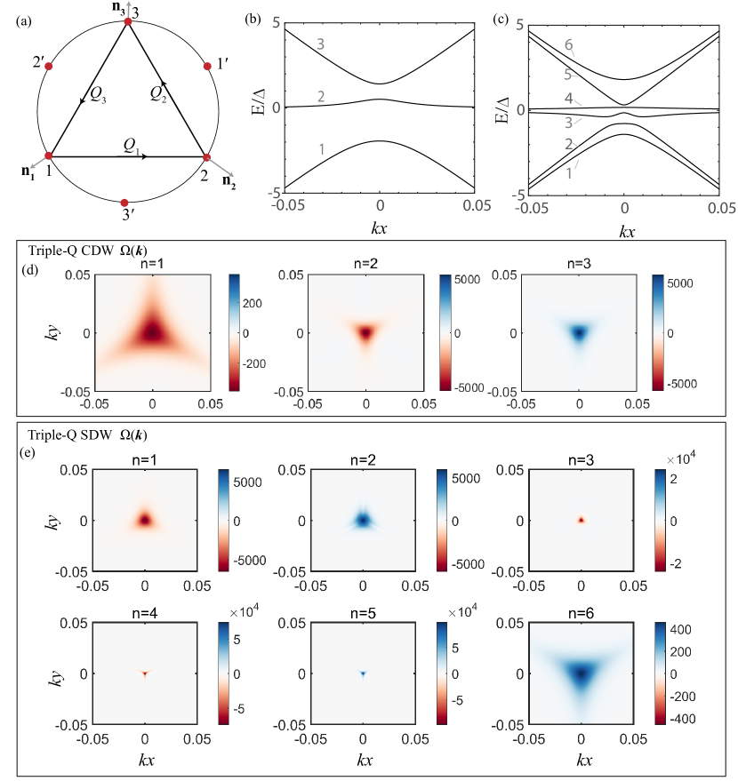
Figure 2: (a) Illustration of the six ‘hot spots’ (red dots) on the Fermi circle, which are connected through the triple-Q vectors. Note that the dispersion of electrons is given by $\xi_{\bm{p}}=\frac{p^{2}}{2m}-\mu$, and $\hat{n}_{i}$ is simply the unit vector for the direction of the hot-spot momentum $\bm{p}_{i}$, where the two density wave order parameters interfere. (b) and (c) respectively, show the band structures of triple-Q CDW and triple-Q SDW along $(k_{x},0)$ direction given by the effective Hamiltonians, where the phase shift is set to be $\theta=\pi/4$. (d) and (f) show the Berry curvature $\Omega(\bm{k})$ (in units of $a^{2}$ and $a$ is the lattice constant) of each band in (b) and (c), respectively. We set $v_{F}=100,\Delta=1$ in calculations. Note that (d) and (e) only show the distribution near one set of hot spots.

Dirac physics induced by triple-Q density waves.— Beyond the real-space topology, next we show that the triple-Q density wave order parameters can alter the geometry properties of Bloch bands using a weak-coupling approach. Specifically, we point out that the triple-Q density waves can spontaneously induce Dirac-like physics near the Fermi energy. As the focus of this work is the triple-Q order parameter, we shall set the band dispersion to be the simplest one: $\xi_{\bm{p}}=\frac{\bm{p}^{2}}{2m}-\mu$, where $m$ is an effective mass, $\mu$ is the chemical potential. In practice, the chemical potential $\mu$ should be located near the Fermi energy where the CDW nesting happens. As shown in Fig. 2(a), there are six ‘hot spots’ (labeled as red dots) that the triple-Q order parameter would couple near Fermi energy. These hot spots can be classified into two sets, i.e., 1,2,3 and 1^′,2^′,3^′. The single-particle dispersion near the hot spots can be approximated as

$$\epsilon_{\bm{k}}=v_{F}\bm{\hat{n}}_{i}\cdot\bm{k},$$ (5)

where $v_{F}$ is the Fermi velocity, and unit vectors $\hat{\bm{n}}_{1}=(-\frac{\sqrt{3}}{2},-\frac{1}{2}),\hat{\bm{n}}_{2}=(\frac{\sqrt{3}}{2},-\frac{1}{2}),\hat{\bm{n}}_{3}=(0,1)$, and the momentum $\bm{k}$ is measured with respect to the hot-spot momentum $\bm{p}_{i}$ with $\bm{k}=\bm{p}-\bm{p}_{i}$.

Next, we present the low-energy effective Hamiltonians with the triple-Q order parameter, which would induce the coupling between these hot spots. Here, we assume the coupling is weak enough so that these hot spots do not overlap with each other. We first focus on the triple-Q CDW. The effective Hamiltonian of the CDW state can be written as $\mathcal{H}=\sum\Phi_{\bm{k}}^{\dagger}H_{\text{CDW}}(\bm{k})\Phi_{\bm{k}}$ with $\Phi_{\bm{k}}=(c_{1\bm{k}},c_{2\bm{k}},c_{3\bm{k}})^{T}$ and

$$H_{\text{CDW}}(\bm{k})=\begin{pmatrix}v_{F}\bm{k}\cdot\hat{\bm{n}}_{1}&\Delta e^{-i\theta}&\Delta e^{i\theta}\\ \Delta e^{i\theta}&v_{F}\bm{k}\cdot\hat{\bm{n}}_{2}&\Delta e^{-i\theta}\\ \Delta e^{-i\theta}&\Delta e^{i\theta}&v_{F}\bm{k}\cdot\hat{\bm{n}}_{3}\end{pmatrix},$$ (6)

where $\bm{k}$ is measured with respect to the hot spots. The effective Hamiltonian $H^{\prime}_{\text{CDW}}(\bm{k})$ defined in the other group $(c_{1^{\prime}\bm{k}},c_{2^{\prime}\bm{k}},c_{3^{\prime}\bm{k}})^{T}$ can be obtained by replacing $\hat{\bm{n}}_{i}$ and $\theta$ in $H_{\text{CDW}}(\bm{k})$ with $\hat{\bm{n}^{\prime}}_{i}=-\hat{\bm{n}}_{i}$ and $-\theta$.

To emphasize the nontrivial band geometry encoded in the effective Hamiltonian, we show that $H_{\text{CDW}}(\bm{k})$ can be actually mapped to a three-band Dirac Hamiltonian [21]. As shown in Supplementary Material (SM) Sec. I [22], the eigenstates of $H_{\text{CDW}}(\bm{k})$ at $\bm{k}=0$ can be labeled with the eigenvalue of $C_{3z}$ operation: $C_{3z}\ket{E_{J,m}}=e^{-i\frac{2m\pi}{3}}\ket{E_{J,m}}$, where the total angular momentum $J=1$, the magnetic angular momentum $m=0,\pm 1$. After projecting the $H_{\text{CDW}}(\bm{k})$ into the ‘good’ basis spanned by $(\ket{E_{1,0}},\ket{E_{1,-1}},\ket{E_{1,1}})$, the effective Hamiltonian is represented as a three-band Dirac Hamiltonian:

$$H_{\text{Dirac}}(\bm{k})=\begin{pmatrix}E_{1,0}&-\frac{i}{2}v_{F}k_{-}&-\frac{i}{2}v_{F}k_{+}\\ \frac{i}{2}v_{F}k_{+}&E_{1,-1}&-\frac{i}{2}v_{F}k_{-}\\ \frac{i}{2}v_{F}k_{-}&\frac{i}{2}v_{F}k_{+}&E_{1,1}\end{pmatrix}$$ (7)

where $k_{\pm}=k_{x}\pm ik_{y}$, $E_{J,m}=2\Delta\cos(\theta-\frac{2m\pi}{3})$, and the phase shift plays a significant role in affecting the Dirac mass.

Table 2: Possible responses induced triple-Q density wave order parameters from symmetry principle. Here, AHE and SHG label the anomalous Hall and second harmonic generation effects, respectively.

	Phase shift	key symmetries	representative responses
Triple-Q CDW	$\theta=\frac{2n\pi}{3}$	$T$, $I$, $C_{3z}$, $M_{x}$, $M_{y}$
	$\theta\neq\frac{2n\pi}{3}$	$T$,$\cancel{I}$, $C_{3z}$, $\cancel{M_{x}}$, $M_{y}$	SHG, Valley Hall effect
Triple-Q SDW	$\theta=\frac{n\pi}{3}$	$\cancel{T}$,$\cancel{I}$, $C_{2z}$, $C_{3z}$	AHE, magnetoptical
	$\theta\neq\frac{n\pi}{3}$	$\cancel{T}$,$\cancel{I}$, $\cancel{C_{2z}}$, $C_{3z}$	AHE, magnetoptical, magnetochiral, SHG

Similar physics can also be induced by the triple-Q SDW order parameters. Specifically, we can first obtain the effective Hamiltonian near the first set of hot spots (1,2, and 3) as

$$H_{\text{SDW}}(\bm{k})=\begin{pmatrix}v_{F}\bm{k}\cdot\hat{\bm{n}}_{1}&\Delta\bm{S}_{-\bm{Q}_{1}}\cdot\bm{\sigma}&\Delta\bm{S}_{\bm{Q}_{3}}\cdot\bm{\sigma}\\ \Delta\bm{S}_{\bm{Q}_{1}}\cdot\bm{\sigma}&v_{F}\bm{k}\cdot\hat{\bm{n}}_{2}&\Delta\bm{S}_{-\bm{Q}_{2}}\cdot\bm{\sigma}\\ \Delta\bm{S}_{-\bm{Q}_{3}}\cdot\bm{\sigma}&\Delta\bm{S}_{\bm{Q}_{2}}\cdot\bm{\sigma}&v_{F}\bm{k}\cdot\hat{\bm{n}}_{3}\end{pmatrix},$$ (8)

where the basis is $(c_{1\bm{k}},c_{2\bm{k}},c_{3\bm{k}})^{T}\otimes(\uparrow,\downarrow)^{T}$, and $\bm{S}_{\pm\bm{Q}_{\nu}}=(\mp\frac{i}{2}\cos\phi_{\nu},\mp\frac{i}{2}\sin\phi_{\nu},\mp\frac{1}{2})e^{i\pm\theta}$. By replacing $\bm{S}_{\pm\bm{Q}_{\nu}}$ with $\bm{S}_{\mp\bm{Q}_{\nu}}$ and $\hat{\bm{n}}_{i}$ with $\hat{\bm{n}}^{\prime}_{i}$, the low-energy Hamiltonian $H^{\prime}_{\text{SDW}}(\bm{k})$ near the other set of hot spots ($1^{\prime}$, $2^{\prime}$, $3^{\prime}$) can be obtained. Also, performing a unitary transform and rewriting the Hamiltonian in the basis $\ket{E}_{J,m}\otimes\{\uparrow,\downarrow\}$, a six-band Dirac-like Hamiltonian can be obtained (see SM. II for the detailed form).

One important property of the Dirac Hamiltonian is to enable the Berry curvature, which has been associated with various topological materials. Here, we show that the triple-Q density wave order parameters can induce Berry curvature on the simplest quadratic band. The band structures given by $H_{\text{CDW}}(\bm{k})$ and $H_{\text{SDW}}(\bm{k})$ are shown Figs. 2(b) and 2(c), respectively. The Berry curvature of these bands can be easily calculated, as shown in Fig. 2(d) for the triple-Q CDW and Fig. 2(e) for the triple-Q SDW. Moreover, we find that the phase shift would affect the Berry curvature significantly. For example, the Berry curvature vanishes at $\theta=\frac{n\pi}{3}$ and $\theta=\frac{(2n+1)\pi}{6}$ for the $H_{\text{CDW}}(\bm{k})$ and $H_{\text{SDW}}(\bm{k})$ respectively, while the latter exactly corresponds to the presence of meron-antimron crystals in real space.

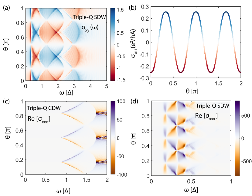
Figure 3: (a) The magnetoptical conductivity $\sigma_{xy}(\omega)$ as a function of the phase shift $\theta$ and the photon frequency $\omega$, where the colorbar is in unit of $\frac{e^{2}}{h}$. (b) The anomalous Hall conductivity as a function of photon frequency. (c) and (d), respectively, show the real part of the second-harmonic response tensor $\text{Re}[\sigma_{xxx}(2\omega;\omega,\omega)]$, which is in units of $e^{3}/(2\hbar^{2})$. The chemical potential in this figure is fixed at the position of hot spots, and the temperature is zero temperature limit with $T=0.01\Delta$.

Linear and nonlinear responses in triple-Q density wave systems.— It is known that the Dirac Hamiltonian plays a critical role in giving rise to various linear and nonlinear responses. According to the analysis in the previous part, we would thus expect that triple-Q density wave order parameters would naturally result in some interesting linear and nonlinear responses as well.

Let us identify the symmetries dedicated by the triple-Q density wave order parameter first. Either from the real-space landscape or the effective Hamiltonian (see SM Sec. I), we can identify the triple-Q CDW order parameter $\Delta_{\text{CDW}}(\bm{r})$ would preserve time-reversal and $C_{3z}$ symmetry at generic $\theta$ but breaks inversion only when $\theta\neq\frac{2n\pi}{3}$. Consequently, a second harmonic generation (SHG) solely induced by the triple-Q CDW would be expected. Furthermore, if we consider the two sets of hotspots within CDWs as distinct valleys within momentum space, the Berry curvature contrasts between these valleys due to time-reversal symmetry. This contrast can induce valley Hall effects. The situation mirrors gapped graphene systems, where valley Hall effects are observable through nonlocal transport phenomena [23, 24] or via valley-selective Hall measurements induced by circular-polarized light [25, 26].

On the other hand, it can be shown that the triple-Q SDW order parameter $\Delta_{\text{SDW}}(\bm{r})$ would break both time-reversal and inversion symmetry regardless of the value of $\theta$ (see SM Sec. II). The broken time-reversal symmetry allows the anomalous Hall effect (AHE) and magnetoptical responses, while the further broken inversion symmetry is crucial for the nonreciprocal or nonlinear responses [27]. The resulting key point group symmetry generators induced by the $\Delta_{\text{SDW}}(\bm{r})$ are $C_{2z}$ and $C_{3z}$ at $\theta=\frac{n\pi}{3}$, and $C_{2z}$ would be broken when $\theta\neq\frac{n\pi}{3}$. Note that, unlike triple-Q CDWs, the point group formed by the unitary operations of triple-Q SDWs is chiral, where all mirror symmetries are broken. The nonreciprocal nonlinear responses such as SHG can thus be induced by triple-Q SDW order as well. To be clear, the above discussions are explicitly summarized in Table II. To be consistent, we still keep $C_{3z}$ here. Note that when the $C_{3z}$ symmetry is absent, such as broken by the external strain, other interesting effects may further be allowed (see SM Sec. III for a discussion of nonlinear Hall effects [28, 29, 30] in strained SDW states).

To be more explicit, we calculate some representative linear and nonlinear responses from the effective triple-Q CDW and SDW Hamiltonians. The representative linear responses: AHE and magnetoptical conductivity can be obtained from the Kubo formula [31]. Using the triple-Q effective Hamiltonian $H_{\text{SDW}}(\bm{k})$ and $H^{\prime}_{\text{SDW}}(\bm{k})$ (these two contributions need to be summed up), the calculated magnetoptical conductivity $\sigma_{xy}(\omega)$ as a function the frequency $\omega$ and the phase shift $\theta$, and the calculated AHE conductivity $\sigma_{\text{AH}}$ versus $\theta$ are shown in Fig. 3 (a) and (b), respectively. The finite AHE and magnetoptical effect are expected due to the nontrivial band geometry near Fermi energy. It is worth noting that the AHE vanishes at $\theta=\frac{(2n+1)\pi}{6}$, while remaining finite at other phase shifts. Such observation is consistent with the real-space topology discussed in Fig. 1: the meron-antimeron crystal appears at $\theta=\frac{(2n+1)\pi}{6}$, while the skyrmion crystals that possess topological Hall effects would appear at other phase shifts.

Finally, we highlight the representative nonlinear responses enabled by the triple-Q density wave order parameters. As we mentioned, both the triple-Q CDW and SDW order parameters can break the inversion symmetry and also induce nontrivial geometric behavior on the Bloch wave function. These behaviors fit the realization of SHG responses well. As a demonstration, the second harmonic generation response tensor $\sigma_{xxx}(2\omega;\omega,\omega)$ calculated from the effective Hamiltonians of triple-Q CDW and SDW are shown in Fig. 3(c) to (d) (see the explicit SHG formalism in refs. [32, 33] or in SM Sec. IV ). Remarkably, the SHG keeps finite at a wide parameter region. Some special phase shifts where the SHG vanishes also match with the expectations: (i) $\theta=\frac{2n\pi}{3}$ for triple-Q CDW due to the restoration of inversion symmetry, (ii) $\theta=\frac{n\pi}{3}$ and $\theta=\frac{(2n+1)\pi}{6}$ for triple-Q CDW and SDW, where the inversion symmetry is still broken but the Berry curvature vanishes. Furthermore, it is worth noting that nonreciprocal nonlinear responses, particularly SHG and magnetochiral anisotropy, have been experimentally studied in several triple-Q density wave systems, such as 1T TiSe₂ [34], kagome metal CsV₃Sb₅ [35] and SkX [36, 37]. We also checked the magnetochiral anisotropy would be supported in tripe-Q SDW at $\theta\neq\frac{n\pi}{3}$ with $C_{2z}$ symmetry broken. Hence, our study here would provide a possible way to explain the experiments [34, 35, 36, 37] from the perspective of triple-Q density waves.

Y.M.X. acknowledges financial support from the RIKEN Special Postdoctoral Researcher (SPDR) Program. N.N. is supported by JSTCREST Grants No.JMPJCR1874.

I Detailed analysis for the Triple-Q CDW state

As shown in Fig. S1 (a) and (b), there are six hot spots connected by the triple-Q vectors. These hot spots can be classified into two groups, i.e., 1,2,3 and 1^′,2^′,3^′. The dispersion $\xi_{\bm{k}}=\frac{\hbar^{2}\bm{k}^{2}}{2m}-\mu$ near the hot spots can be approximated as

$$\xi_{\bm{k}}=v_{F}\bm{\hat{n}}_{i}\cdot\bm{k},$$ (S1)

where $v_{F}$ is the Fermi velocity, and

$$\hat{\bm{n}}_{1}=(-\frac{\sqrt{3}}{2},-\frac{1}{2}),\hat{\bm{n}}_{2}=(\frac{\sqrt{3}}{2},-\frac{1}{2}),\hat{\bm{n}}_{3}=(0,1).$$ (S2)

In real space, the CDW order parameters can be written as

$$\Delta(\bm{r}_{i})=2\Delta\sum_{\nu}\cos(\bm{Q}_{\nu}\cdot\bm{r}_{i}+\theta_{\nu}).$$ (S3)

Here,

$$\bm{Q}_{1}=(Q,0),\bm{Q}_{2}=(-Q/2,\sqrt{3}Q/2),\bm{Q}_{3}=(-Q/2,-\sqrt{3}Q/2).$$ (S4)

The effective Hamiltonian of the CDW state can be written as $\mathcal{H}=\sum\Phi_{\bm{k}}^{\dagger}H_{\text{CDW}}(\bm{k})\Phi_{\bm{k}}$ with $\Phi_{\bm{k}}=(c_{1\bm{k}},c_{2\bm{k}},c_{3\bm{k}})^{T}$ and

$$H_{\text{CDW}}(\bm{k})=\begin{pmatrix}v_{F}\bm{k}\cdot\hat{\bm{n}}_{1}&\Delta e^{-i\theta_{1}}&\Delta e^{i\theta_{3}}\\ \Delta e^{i\theta_{1}}&v_{F}\bm{k}\cdot\hat{\bm{n}}_{2}&\Delta e^{-i\theta_{2}}\\ \Delta e^{-i\theta_{3}}&\Delta e^{i\theta_{2}}&v_{F}\bm{k}\cdot\hat{\bm{n}}_{3}\end{pmatrix},$$ (S5)

where $\bm{k}$ is measured respected from $\bm{K}_{i}$. Near the other group hot spots, the effective Hamiltonian becomes

$$H^{\prime}_{\text{CDW}}(\bm{k})=\begin{pmatrix}v_{F}\bm{k}\cdot\hat{\bm{n}}^{\prime}_{1}&\Delta e^{i\theta_{1}}&\Delta e^{-i\theta_{3}}\\ \Delta e^{-i\theta_{1}}&v_{F}\bm{k}\cdot\hat{\bm{n}}^{\prime}_{2}&\Delta e^{i\theta_{2}}\\ \Delta e^{i\theta_{3}}&\Delta e^{-i\theta_{2}}&v_{F}\bm{k}\cdot\hat{\bm{n}}^{\prime}_{3}\end{pmatrix}$$ (S6)

Next, let us deduce the symmetry operations for the effective Hamiltonian. First of all, it is easy to show that the system respects the spinless time-reversal symmetry $\mathcal{T}=K$ ($K$ the conjugate)

$$\mathcal{T}H^{\prime}_{\text{CDW}}(-\bm{k})\mathcal{T}^{-1}=H_{\text{CDW}}(\bm{k}).$$ (S7)

The representation of out-of-plane three-fold rotation can be written as

$$U_{C_{3}}=\begin{pmatrix}0&1&0\\ 0&0&1\\ 1&0&0\end{pmatrix}.$$ (S8)

Then it is straightforward to show that under the $C_{3}$ operation,

$$U_{C_{3}}H_{\text{CDW}}(C_{3}\bm{k})U_{C_{3}}^{-1}=\begin{pmatrix}v_{F}\bm{k}\cdot\hat{\bm{n}}_{1}&\Delta e^{-i\theta_{2}}&\Delta e^{i\theta_{1}}\\ \Delta e^{-i\theta_{3}}&v_{F}\bm{k}\cdot\hat{\bm{n}}_{2}&\Delta e^{-i\theta_{3}}\\ \Delta e^{-i\theta_{1}}&\Delta e^{i\theta_{3}}&v_{F}\bm{k}\cdot\hat{\bm{n}}_{3}\end{pmatrix}.$$ (S9)

We can see that the system preserves $C_{3}$ symmetry $U_{C_{3}}H_{\text{CDW}}(C_{3}\bm{k})U_{C_{3}}^{-1}=H_{\text{CDW}}(C_{3}\bm{k})$ if $\theta_{1}=\theta_{2}=\theta_{3}=\theta$. Similarly, $U_{C_{3}}H^{\prime}_{\text{CDW}}(C_{3}\bm{k})U_{C_{3}}^{-1}=H^{\prime}_{\text{CDW}}(C_{3}\bm{k})$ so that the full system respects $C_{3}$ symmetry. Hence, we would fix the $\theta_{1}=\theta_{2}=\theta_{3}$ in our discussion.

Furthermore, when $\theta=\frac{2n\pi}{3}$ ($n$ are integers), the system further respects the inversion symmetry and $M_{x}$:

$$IH^{\prime}_{\text{CDW}}(-\bm{k})I^{-1} =H_{\text{CDW}}(\bm{k}),$$ (S10)

$$M_{x}H_{\text{CDW}}(-k_{x},k_{y})M_{x}^{-1} =H_{\text{CDW}}(k_{x},k_{y}),$$ (S11)

Note that the effects of inversion and out-of-plane $C_{2}$ are the same here. Finally, for all $\theta$, the system exhibits $M_{y}$ symmetry:

$$M_{y}H_{\text{CDW}}(k_{x},-k_{y})M_{y}^{-1}=H^{\prime}_{\text{CDW}}(k_{x},k_{y}).$$ (S12)

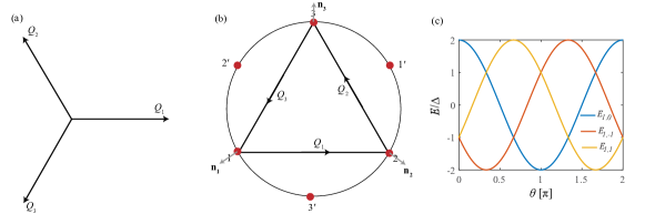
Figure S1: (a) Triple Q vectors: $\bm{Q}_{1}$, $\bm{Q}_{2}$, $\bm{Q}_{3}$. (b) Six hot spots in k-space, where the gap opening due to density waves overlap. These six hot spots can be classified into two groups:(1,2,3) and (1^′,2^′,3^′). (c) The energy $E_{J,m}$ versus $\theta$ with $J=1$, $m=0,\pm 1$.

In the main text, we have mapped $H_{\text{CDW}}(\bm{k})$ as a three-band massive Dirac Hamiltonian. Now we present the details here. We can solve the eigenstates and eigenenergies of $H(\bm{k})$ analytically at the hot spots ($\bm{k}=0$):

$$E_{1,0} =2\Delta\cos\theta,\ket{E_{1,0}}=\frac{1}{\sqrt{3}}(\ket{\kappa_{1}}+\ket{\kappa_{2}}+\ket{\kappa_{3}}),$$ (S13)

$$E_{1,-1} =2\Delta\cos(\frac{2\pi}{3}+\theta),\ket{E_{1,-1}}=\frac{1}{\sqrt{3}}(e^{i\frac{\pi}{3}}\ket{\kappa_{1}}+e^{-i\frac{\pi}{3}}\ket{\kappa_{2}}+e^{i\pi}\ket{\kappa_{3}}),$$ (S14)

$$E_{1,1} =2\Delta\cos(\frac{4\pi}{3}+\theta),\ket{E_{1,1}}=\frac{1}{\sqrt{3}}(e^{i\frac{2\pi}{3}}\ket{\kappa_{1}}+e^{i\frac{4\pi}{3}}\ket{\kappa_{2}}+\ket{\kappa_{3}}).$$ (S15)

where we have labeled the eigenstates as $E_{J,m}$ with $J$ as the total angular momentum number, $m$ as the magnetic quantum number. It is easy to verify that $C_{3}\ket{E_{J,m}}=e^{-i\frac{2m\pi}{3}}\ket{E_{J,m}}$ under the splinless $C_{3}$ operation. Then we can project the Hamiltonian in the basis spanned by $(\ket{E_{1,0}},\ket{E_{1,-1}},\ket{E_{1,1}})$:

$$U_{0}^{\dagger}H_{\text{CDW}}(\bm{k})U_{0}=H_{0}(\bm{k})=\begin{pmatrix}E_{1,0}&-\frac{i}{2}v_{F}(k_{x}-ik_{y})&-\frac{i}{2}v_{F}(k_{x}+ik_{y})\\ \frac{i}{2}v_{F}(k_{x}+ik_{y})&E_{1,-1}&-\frac{i}{2}v_{F}(k_{x}-ik_{y})\\ \frac{i}{2}v_{F}(k_{x}-ik_{y})&\frac{i}{2}v_{F}(k_{x}+ik_{y})&E_{1,1}\end{pmatrix},$$ (S16)

where

$$U_{0}=\frac{1}{\sqrt{3}}\begin{pmatrix}1&e^{i\frac{\pi}{3}}&e^{i\frac{2\pi}{3}}\\ 1&e^{-i\frac{\pi}{3}}&e^{i\frac{4\pi}{3}}\\ 1&-1&1\end{pmatrix}.$$ (S17)

It can be seen that Eq. (S16) is equivalent to the main text Eq. (7).

II Detailed analysis for the triple-Q SDW state case

As mentioned in the main text, we can express the SDW states with the superposition of spiral spin textures

$$\bm{S}_{i}^{spiral}=\Delta\sum_{\nu=1}^{3}(\sin\mathcal{Q}_{\nu}\cos\phi_{\nu},\sin\mathcal{Q}_{\nu}\sin\phi_{\nu},-\cos\mathcal{Q}_{\nu}).$$ (S18)

where $i$ is the site index, $\phi_{\nu}=\frac{2}{3}\pi(\nu-1)$, $\mathcal{Q}_{\nu}=\bm{Q}_{\nu}\cdot\bm{r}_{i}+\theta_{\nu}$.

It is easy to verify that the Zeeman Hamiltonian caused by the SDW states is $C_{3}$ invariant:

$$H_{Z}=\sum_{i}\bm{S}_{i}^{spiral}\cdot\bm{\sigma}.$$ (S19)

Then, we can obtain the effective Hamiltonian near the first group hot spots (1,2, and 3) as

$$H_{\text{SDW}}(\bm{k})=\begin{pmatrix}v_{F}\bm{k}\cdot\bm{n}_{1}&\Delta\bm{S}_{-\bm{Q}_{1}}\cdot\bm{\sigma}&\Delta\bm{S}_{\bm{Q}_{3}}\cdot\bm{\sigma}\\ \Delta\bm{S}_{\bm{Q}_{1}}\cdot\bm{\sigma}&v_{F}\bm{k}\cdot\bm{n}_{2}&\Delta\bm{S}_{-\bm{Q}_{2}}\cdot\bm{\sigma}\\ \Delta\bm{S}_{-\bm{Q}_{3}}\cdot\bm{\sigma}&\Delta\bm{S}_{\bm{Q}_{2}}\cdot\bm{\sigma}&v_{F}\bm{k}\cdot\bm{n}_{3}\end{pmatrix}.$$ (S20)

where the basis is $(c_{1\bm{k},\uparrow},c_{1\bm{k},\downarrow},c_{2\bm{k},\uparrow},c_{2\bm{k},\downarrow},c_{3\bm{k},\uparrow},c_{3\bm{k},\downarrow})^{T}$, and

$$\bm{S}_{\bm{Q}_{\nu}} =(-\frac{i}{2}\cos\phi_{\nu},-\frac{i}{2}\sin\phi_{\nu},-\frac{1}{2})e^{i\theta_{\nu}},$$ (S21)

$$\bm{S}_{-\bm{Q}_{\nu}} =(\frac{i}{2}\cos\phi_{\nu},\frac{i}{2}\sin\phi_{\nu},-\frac{1}{2})e^{-i\theta_{\nu}}.$$ (S22)

Near the second group hot spots (1^′, 2^′, and 3^′), the effective Hamiltonian is

$$H^{\prime}_{\text{SDW}}(\bm{k})=\begin{pmatrix}v_{F}\bm{k}\cdot\bm{n}^{\prime}_{1}&\Delta\bm{S}_{\bm{Q}_{1}}\cdot\bm{\sigma}&\Delta\bm{S}_{-\bm{Q}_{3}}\cdot\bm{\sigma}\\ \Delta\bm{S}_{-\bm{Q}_{1}}\cdot\bm{\sigma}&v_{F}\bm{k}\cdot\bm{n}^{\prime}_{2}&\Delta\bm{S}_{\bm{Q}_{2}}\cdot\bm{\sigma}\\ \Delta\bm{S}_{\bm{Q}_{3}}\cdot\bm{\sigma}&\Delta\bm{S}_{-\bm{Q}_{2}}\cdot\bm{\sigma}&v_{F}\bm{k}\cdot\bm{n}^{\prime}_{3}\end{pmatrix}$$ (S23)

Again, if $\theta=\theta_{1}=\theta_{2}=\theta_{3}$, we can easily show that the system respects the out-of-plane $C_{3z}$ symmetry with

$$U_{C_{3z}}H_{\text{SDW}}(C_{3}\bm{k})U_{C_{3z}}^{-1}=H_{\text{SDW}}(\bm{k}),U_{C_{3z}}H^{\prime}_{\text{SDW}}(C_{3}\bm{k})U_{C_{3z}}^{-1}=H^{\prime}_{\text{SDW}}(\bm{k}),$$ (S24)

where the representation of $C_{3}$ operation is

$$U_{C_{3}}=\begin{pmatrix}0&1&0\\ 0&0&1\\ 1&0&0\end{pmatrix}\otimes e^{-i\frac{\pi}{3}\sigma_{z}}.$$ (S25)

When $\theta=n\pi$ with $n$ as integers, we find there is an out-of-plan $C_{2z}$ symmetry. It can be seen that the system breaks the time-reversal symmetry $\hat{T}=i\sigma_{y}K$, which can be seen from

$$\hat{T}H^{\prime}_{\text{SDW}}(-\bm{k})\hat{T}^{-1}\neq H_{\text{SDW}}(\bm{k}).$$ (S26)

The inversion symmetry is also broken in general:

$$\hat{I}H^{\prime}_{\text{SDW}}(-\bm{k})\hat{I}^{-1}\neq H_{\text{SDW}}(\bm{k}).$$ (S27)

But there is an emergent ‘particle-hole’ symmetry:

$$H_{\text{SDW}}(\bm{k})=-\hat{T}H^{\prime}_{SDW}(\bm{k})\hat{T}^{-1},$$ (S28)

and it respects the combined symmetry $\hat{M}_{y}\hat{T}$ for arbitrary $\theta$ with

$$U_{\hat{M}_{y}\hat{T}}=\begin{pmatrix}0&-i\sigma_{y}&0\\ -i\sigma_{y}&0&0\\ 0&0&-i\sigma_{y}\end{pmatrix}i\sigma_{y}K=\begin{pmatrix}0&\sigma_{0}&0\\ \sigma_{0}&0&0\\ 0&0&\sigma_{0}\end{pmatrix}K$$ (S29)

and

$$U_{\hat{M}_{y}\hat{T}}H_{\text{SDW}}(-k_{x},k_{y})U_{\hat{M}_{y}\hat{T}}^{-1}=H_{\text{SDW}}(k_{x},k_{y}).$$ (S30)

The full form of the Hamiltonian is

$$H_{\text{SDW}}(\bm{k})=\begin{pmatrix}v_{F}(-\frac{\sqrt{3}}{2}k_{x}-\frac{1}{2}k_{y})&\Delta(\frac{i}{2}\sigma_{x}-\frac{1}{2}\sigma_{z})e^{-i\theta}&\Delta(\frac{i}{4}\sigma_{x}+\frac{\sqrt{3}}{4}i\sigma_{y}-\frac{1}{2}\sigma_{z})e^{i\theta}\\ \Delta(-\frac{i}{2}\sigma_{x}-\frac{1}{2}\sigma_{z})e^{i\theta}&v_{F}(\frac{\sqrt{3}}{2}k_{x}-\frac{1}{2}k_{y})&\Delta(-\frac{i}{4}\sigma_{x}+\frac{\sqrt{3}}{4}i\sigma_{y}-\frac{1}{2}\sigma_{z})e^{-i\theta}\\ \Delta(-\frac{i}{4}\sigma_{x}-\frac{\sqrt{3}}{4}i\sigma_{y}-\frac{1}{2}\sigma_{z})e^{-i\theta}&\Delta(\frac{i}{4}\sigma_{x}-\frac{\sqrt{3}}{4}i\sigma_{y}-\frac{1}{2}\sigma_{z})e^{i\theta}&v_{F}k_{y}\end{pmatrix}.$$ (S31)

$$H^{\prime}_{\text{SDW}}(\bm{k})=\begin{pmatrix}v_{F}(\frac{\sqrt{3}}{2}k_{x}+\frac{1}{2}k_{y})&\Delta(-\frac{i}{2}\sigma_{x}-\frac{1}{2}\sigma_{z})e^{i\theta}&\Delta(-\frac{i}{4}\sigma_{x}-\frac{\sqrt{3}}{4}i\sigma_{y}-\frac{1}{2}\sigma_{z})e^{-i\theta}\\ \Delta(\frac{i}{2}\sigma_{x}-\frac{1}{2}\sigma_{z})e^{-i\theta}&v_{F}(-\frac{\sqrt{3}}{2}k_{x}+\frac{1}{2}k_{y})&\Delta(\frac{i}{4}\sigma_{x}-\frac{\sqrt{3}}{4}i\sigma_{y}-\frac{1}{2}\sigma_{z})e^{i\theta}\\ \Delta(\frac{i}{4}\sigma_{x}+\frac{\sqrt{3}}{4}i\sigma_{y}-\frac{1}{2}\sigma_{z})e^{i\theta}&\Delta(-\frac{i}{4}\sigma_{x}+\frac{\sqrt{3}}{4}i\sigma_{y}-\frac{1}{2}\sigma_{z})e^{-i\theta}&-v_{F}k_{y}\end{pmatrix}.$$ (S32)

It is easy to see that

$$C_{2z}H_{\text{SDW}}(\bm{k},\theta)C_{2z}^{-1}=H^{\prime}_{\text{SDW},\theta=0}(-\bm{k},-\theta).$$ (S33)

Hnece, the $C_{2z}$ symmetry is here when $\theta=n\pi$, and due to $C_{3Z}$ symmetry, the system further would respect $C_{2z}$ symmetry at $\theta=\frac{n\pi}{3}$:

$$C_{2z}H_{\text{SDW}}(\bm{k},\theta=\frac{n\pi}{3})C_{2z}^{-1}=H^{\prime}_{\text{SDW},\theta=n\pi}(-\bm{k},\theta=\frac{n\pi}{3}).$$ (S34)

In other words, the point group of this triple-Q SDW is $C_{6}$ at $\theta=\frac{n\pi}{3}$ and reduces to $C_{3}$ at other angles.

We can perform a unitary transform and rewrite the Hamiltonian in the basis $(\ket{E_{1,0}}\otimes\ket{\uparrow},\ket{E_{1,1}}\otimes\ket{\downarrow},\ket{E_{1,-1}}\otimes\ket{\uparrow},\ket{E_{1,0}}\otimes\ket{\downarrow},\ket{E_{1,1}}\otimes\ket{\uparrow},\ket{E_{1,-1}}\otimes\ket{\downarrow})^{T}$, which carries the eigenvalues of $(e^{-i\frac{\pi}{3}},e^{-i\frac{\pi}{3}},e^{i\frac{\pi}{3}},e^{i\frac{\pi}{3}},1,1)$ under $C_{3}$ operation.

$$H(\bm{k})=\begin{pmatrix}H_{11}&-\frac{i}{2}(k_{x}-ik_{y})\sigma_{z}&-\frac{i}{2}(k_{x}-ik_{y})\sigma_{z}\\ \frac{i}{2}(k_{x}+ik_{y})\sigma_{z}&H_{22}&-\frac{i}{2}(k_{x}-ik_{y})\sigma_{0}\\ \frac{i}{2}(k_{x}+ik_{y})\sigma_{z}&\frac{i}{2}(k_{x}+ik_{y})\sigma_{0}&H_{33}\end{pmatrix},$$ (S35)

where the terms

$$H_{11} =-\frac{\sqrt{3}}{2}\Delta\cos(\theta+\frac{\pi}{6})\sigma_{0}+\Delta\cos(\theta+\frac{\pi}{6})\sigma_{x}-\frac{\Delta}{2}\sin(\theta+\frac{\pi}{6})\sigma_{z},$$ (S36)

$$H_{22} =\frac{\sqrt{3}}{2}\Delta\cos(\theta-\frac{\pi}{6})\sigma_{0}+\Delta\cos(\theta-\frac{\pi}{6})\sigma_{x}+\frac{\Delta}{2}\sin(\theta-\frac{\pi}{6})\sigma_{z},$$ (S37)

$$H_{33} =-\frac{\sqrt{3}}{2}\Delta\sin\theta\sigma_{0}-\Delta\sin\theta\sigma_{x}+\frac{\Delta}{2}\cos\theta\sigma_{z}.$$ (S38)

III Nonreciprocal transports in triple-Q SDWs

III.1 Magnetochiral anisotropy in triple-Q SDWs

We consider a time-dependent drive

$$\mathcal{E}(t)=\bm{E}\cos(\omega t).$$ (S39)

Without loss of generality, we set the electric field $\bm{E}$ along $x$-direction. In the experiment, it is convenient to identify the magnetochiral anisotropy by measuring the second harmonic generation of longitudinal conductivity [36]. Following the previous works [38, 39], it can be deduced that the nonreciprocal longitudinal charge transport can be given by

$$\sigma_{\alpha\alpha\alpha}^{2\omega}=-\frac{e^{3}}{2\hbar^{3}(2i\omega+\tau^{-1})(i\omega+\tau^{-1})}\int\frac{d\bm{k}}{(2\pi)^{d}}\sum_{n}f_{n}^{(0)}\frac{\partial^{3}\epsilon_{n}^{(0)}}{\partial k_{\alpha}^{3}}-\frac{2e^{3}}{\hbar}\int\frac{d\bm{k}}{(2\pi)^{d}}f_{n}^{(0)}\partial_{k_{\alpha}}G_{n}^{\alpha\alpha}(2\omega)$$ (S40)

where $f_{n}^{(0)}$ is the Fermi distribution for the n-th band $\epsilon^{(0)}_{n}$, and the band-renormalized quantum metric is defined as

$$G_{n}^{ab}(2\omega)=-\frac{1}{4}\sum_{l\neq n}(\frac{\mathcal{A}_{nl}^{a}\mathcal{A}_{ln}^{b}}{-\hbar\omega+\epsilon_{ln}}+\frac{\mathcal{A}^{b}_{nl}\mathcal{A}^{a}_{ln}}{\hbar\omega+\epsilon_{ln}}).$$ (S41)

Here, $A^{a}_{mn}=\frac{\braket{n\bm{k}}{\partial_{a}H}{m\bm{k}}}{\epsilon_{nm}}$ denotes the Berry connection between $n-$th and $l-$th band with $\epsilon_{nm}=\epsilon^{(0)}_{n}-\epsilon^{(0)}_{m}$. In the DC transport limit, we are interested in $\omega\rightarrow 0$. In this case, the additional antiunitary symmetry $\hat{M}_{y}\hat{T}$ in triple-Q SDW would enforce $\sigma_{xxx}^{2\omega}=0$ by mapping $k_{x}$ to -$k_{x}$. Instead, we would focus on $\sigma_{yyy}^{2\omega}$ below. The results are summarized in Fig. S2. It can be seen from (a) and (b) that $\sigma_{yyy}^{2\omega}$ is generally finite expect for at $\theta=\frac{n\pi}{3}$ due to the presence of $C_{2z}$ symmetry. Note that we also find that the quantum metric contribution in Eq. S40 is negligible.

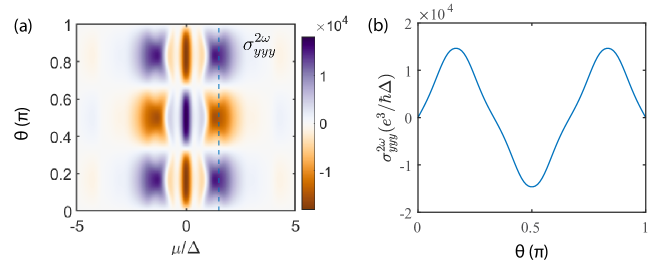
Figure S2: The magnetochiral anisotropy represented by the strength of $\sigma^{2\omega}_{yyy}$ (in units of $\frac{e^{3}}{\hbar\Delta}$).(a) the phase shift dependence and chemical potential dependence of $\sigma_{yyy}^{2\omega}$ calculated from the SDW effective Hamiltonian. (b) A line-cut of (a) at a fixed $\mu=1.5\Delta$. Here, the used parameters are $v_{F}=100$, $\Delta=1$, $T=0.01\Delta$, $\tau=0.01\Delta/\hbar$.

III.2 Possible nonlinear Hall effects in strained triple-Q SDWs

Table S1: Symmetry classification of momentum, spin, and strain tensor according to the irreducible representations of $C_{3}$ point group.

Irrep	Time-reversal Even	Time-reversal odd
$A_{1}$	$u_{xx}+u_{yy}$	$\sigma_{z}$
$E$	($u_{xx}-u_{yy}$,$-2u_{xy}$)	$(k_{x},k_{y})$, $(\sigma_{x},\sigma_{y})$

In the main text, we mostly focus on the $C_{3}$ invariant case. However, the $C_{3}$ symmetry can be broken externally. The question is whether any interesting effects are allowed in this case. In this Supplementary Material section, we demonstrate that the nonlinear Hall effects are possible in strained triple-Q SDWs, such as strained SkX.

To the leading order terms, as shown in Table SI, the time-reversal invariant strain Hamiltonian is

$$H_{strain}=v_{F}\sum_{\alpha\alpha}u_{\alpha}\Gamma_{0}\otimes\sigma_{0}+v_{F}[(u_{xx}-u_{yy})k_{x}-2u_{xy}k_{y}]\Gamma_{0}\otimes\sigma_{z},$$ (S42)

where $\Gamma_{0}$ is a three-by-three identify matrix in the hot spots space, the other group takes the same form. The first term is to effectively shift the chemical potential so we can neglect it. The strain Hamiltonian is simplified as

$$H_{strain}\approx v_{F}[(u_{xx}-u_{yy})k_{x}-2u_{xy}k_{y}]\Gamma_{0}\otimes\sigma_{z}.$$ (S43)

Without loss of generality, we can consider the uniaxial strain tensor to be

$$\begin{pmatrix}u_{xx}&u_{xy}\\ u_{yx}&u_{yy}\end{pmatrix}=u^{\prime}\begin{pmatrix}\cos^{2}\varphi-\nu\sin^{2}\varphi&(1+\nu)\cos\varphi\sin\varphi\\ (1+\nu)\cos\varphi\sin\varphi&-\nu\cos^{2}\varphi+\sin^{2}\varphi\end{pmatrix}$$ (S44)

where $\varphi$ is to label the strain direction, $\nu$ is the Poisson ratio.

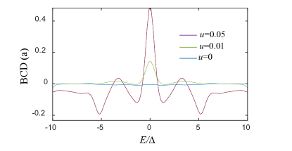
[h]

Figure S3: Nonlinear Hall effects in strained SDW crystals. The Berry curvature dipole (BCD) versus the energy $E$, where $E$ is artificially tuned from $[-10,10]\Delta$ and $E=0$ is the Fermi energy. The strain strength is characterized by $u=0.05,0.01,0$, respectively. It can be seen that the BCD vanishes without strain due to the presence of $C_{3}$ symmetry, while there appears a sizable Berry curvature dipole when the SDW crystal is strained. Here, the used parameters in the triple-Q SDW effective Hamiltonian are $\Delta=1$, $v_{F}=100\Delta$, $\theta=0$, $\mu=0$.

For simplicity, we set $\varphi=\pi/4$, and $u=(1+\nu)u^{\prime}$, the strain Hamiltonian becomes

$$H_{strain}\approx-v_{F}uk_{y}\Gamma_{0}\otimes\sigma_{z},$$ (S45)

where $u$ characterizes the strain strength. Note that $u\neq 0$, the three-fold symmetry is broken. Then we can add the strain Hamiltonian into the total triple-Q Hamiltonian (note that we need to consider two sets of hot spots). The Berry curvature dipole is given by [28]

$$D_{\beta\gamma}=-\sum_{n}\int\frac{d\bm{k}}{(2\pi)^{d}}\frac{\partial\epsilon_{n\bm{k}}}{\partial\bm{k}_{\beta}}\Omega_{n\gamma}(\bm{k})\frac{\partial f(\epsilon_{n\bm{k}})}{\partial\epsilon_{n\bm{k}}}.$$ (S46)

The calculated strained induced finite Berry curvature dipole $D_{yz}$ is shown in Fig. S3. It can be seen that there can support finite Berry curvature dipole in strained triple-Q SDW systems.

IV second harmonic generation responses formalism

We reproduce the optical responses formula given by ref. [32, 33] here, which has been used in the main text to calculate the SHG below. The linear optical conductivity is given by the bubble diagram [Fig. S3(a)],

$$\sigma^{\mu\alpha}(\omega;\omega) =\frac{ie^{2}}{\hbar\omega_{1}}\sum_{a\neq b}\int[d\bm{k}]\int d\omega^{\prime}G_{a}(\omega^{\prime})v_{ab}^{\alpha}G_{b}(\omega^{\prime}+\omega_{1})v_{ba}^{\mu}$$ (S47)

$$=\frac{ie^{2}}{\hbar\omega}\sum_{a\neq b}\int[d\bm{k}]\frac{f_{ab}v_{ab}^{\alpha}v_{ba}^{\mu}}{\omega-\epsilon_{ba}}.$$

where $[d\bm{k}]=\int\frac{d\bm{k}}{(2\pi)^{d}}$, $v_{ab}^{\alpha}=\braket{a}{\partial_{k_{\alpha}}H(\bm{k})}{b}$, $H(\bm{k})$ is the Hamiltonian, the Fermi Dirac function difference between two bands $f_{ab}=f_{a}-f_{b}$, $\epsilon_{ba}=\epsilon_{b}-\epsilon_{a}$.

As shown in Fig. S3, the second-order nonlinear optical conductivity is given by

$$\sigma^{\mu\alpha\beta}(\omega_{1}+\omega_{2};\omega_{1},\omega_{2}) =-\frac{e^{3}}{2\hbar^{2}\omega_{1}\omega_{2}}\sum_{a,b,c}\int[d\bm{k}]\int d\omega^{\prime}[G_{a}(\omega^{\prime})v_{ab}^{\alpha}G_{b}(\omega^{\prime}+\omega_{1})v_{ba}^{\mu\beta}+\frac{1}{2}G_{a}(\omega^{\prime})v_{ab}^{\alpha\beta}G_{b}(\omega^{\prime}+\omega_{1}+\omega_{2})v_{ba}^{\mu}+$$ (S48)

$$G_{a}(\omega^{\prime})v_{ab}^{\alpha}G_{b}(\omega^{\prime}+\omega_{1})v_{bc}^{\beta}G_{c}(\omega^{\prime}+\omega_{1}+\omega_{2})v^{\mu}_{ca}]+(\omega_{1},\alpha)\leftrightarrow(\omega_{2},\beta),$$

$$=-\frac{e^{3}}{2\hbar^{2}\omega_{1}\omega_{2}}\int[d\bm{k}][f_{ab}(\frac{v_{ab}^{\alpha}v_{ba}^{\mu\beta}}{\omega_{1}-\epsilon_{ba}}+\frac{v_{ab}^{\beta}v_{ba}^{\mu\alpha}}{\omega_{2}-\epsilon_{ba}})+f_{ab}\frac{v_{ab}^{\alpha\beta}v_{ba}^{\mu}}{\omega_{1}+\omega_{2}-\epsilon_{ab}}$$

$$+v_{ab}^{\alpha}v_{bc}^{\beta}v_{ca}^{\mu}(\frac{f_{ab}}{(\omega_{1}-\epsilon_{ba})(\omega_{1}+\omega_{2}-\epsilon_{ca})}+\frac{f_{cb}}{(\omega_{2}-\epsilon_{cb})(\omega_{1}+\omega_{2}-\epsilon_{ca})})$$

$$+v_{ab}^{\beta}v_{bc}^{\alpha}v_{ca}^{\mu}(\frac{f_{ab}}{(\omega_{2}-\epsilon_{ba})(\omega_{1}+\omega_{2}-\epsilon_{ca})}+\frac{f_{cb}}{(\omega_{1}-\epsilon_{cb})(\omega_{1}+\omega_{2}-\epsilon_{ca})})].$$

Here, $v_{ab}^{\alpha\beta}=\braket{a}{\partial_{k_{\alpha}}\partial_{k_{\beta}}H(\bm{k})}{b}$. For the second-harmonic generation ($\omega_{1}=\omega_{2}=\omega$),

$$\sigma^{\mu\alpha\beta}(2\omega;\omega,\omega)=-\frac{e^{3}}{2\hbar^{2}\omega^{2}}\sum_{a,b,c}\int[d\bm{k}][f_{ab}\frac{v_{ab}^{\alpha}v_{ba}^{\mu\beta}+v_{ab}^{\beta}v_{ba}^{\mu\alpha}}{\omega-\epsilon_{ba}}+f_{ab}\frac{v_{ab}^{\alpha\beta}v_{ba}^{\mu}}{2\omega-\epsilon_{ab}}$$

$$+(v_{ab}^{\alpha}v_{bc}^{\beta}+v_{ab}^{\beta}v_{bc}^{\alpha})v_{ca}^{\mu}(\frac{f_{ab}}{(\omega-\epsilon_{ba})(2\omega-\epsilon_{ca})}+\frac{f_{cb}}{(\omega-\epsilon_{cb})(2\omega-\epsilon_{ca})})]$$ (S49)

Using the identity:

$$\frac{f_{ab}}{(\omega-\epsilon_{ba})(2\omega-\epsilon_{ca})}+\frac{f_{cb}}{(\omega-\epsilon_{cb})(2\omega-\epsilon_{ca})}=\frac{1}{\epsilon_{ab}+\epsilon_{cb}}[\frac{2f_{ac}}{2\omega-\epsilon_{ca}}+\frac{f_{cb}}{\omega-\epsilon_{cb}}+\frac{f_{ba}}{\omega-\epsilon_{ba}}].$$ (S50)

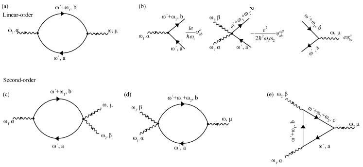
Figure S4: (a) The bubble diagram for the linear optical responses. (b) The vortex diagrams. (c) to (e) The Feynman diagrams for the second-order nonlinear optical response.

The optical conductivity for the second-harmonic generation can be rewritten as

$$\sigma^{\mu\alpha\beta} =\sigma_{\text{I}}^{\mu\alpha\beta}+\sigma_{\text{II}}^{\mu\alpha\beta},$$ (S51)

$$\sigma_{\text{I}}^{\mu\alpha\beta} =-\frac{e^{3}}{2\hbar^{2}\omega^{2}}\sum_{a\neq b}\int[d\bm{k}]f_{ab}\frac{v_{ab}^{\alpha}v_{ba}^{\mu\beta}+v_{ab}^{\beta}v_{ba}^{\mu\alpha}}{\omega-\epsilon_{ba}}+f_{ab}\frac{v_{ab}^{\alpha\beta}v_{ba}^{\mu}}{2\omega-\epsilon_{ab}},$$ (S52)

$$\sigma_{\text{II}}^{\mu\alpha\beta} =-\frac{e^{3}}{2\hbar^{2}\omega^{2}}\sum_{a\neq b\neq c}\int[d\bm{k}]\frac{(v_{ab}^{\alpha}v_{bc}^{\beta}+v_{ab}^{\beta}v_{bc}^{\alpha})v_{ca}^{\mu}}{\epsilon_{ab}+\epsilon_{cb}}(\frac{2f_{ac}}{2\omega-\epsilon_{ca}}+\frac{f_{cb}}{\omega-\epsilon_{cb}}+\frac{f_{ba}}{\omega-\epsilon_{ba}}),$$ (S53)

where $2\omega$ and $\omega$ characterize the contributions from two-photon and one-photon processes, respectively. The contribution that involves two (three) different bands is labeled as $\sigma_{\text{I}}^{\mu\alpha\beta}$ ($\sigma_{\text{II}}^{\mu\alpha\beta}$), respectively.

References

Supplementary Material for “Phase shifts, band geometry and responses in triple-Q charge and spin density waves”
Ying-Ming Xie 1 and Naoto Nagaosa1
1 RIKEN Center for Emergent Matter Science (CEMS), Wako, Saitama 351-0198, Japan