Stochastic Sampling for Contrastive Views and Hard Negative Samples in Graph-based Collaborative Filtering

Abstract.

Graph-based collaborative filtering (CF) has emerged as a promising approach in recommendation systems. Despite its achievements, graph-based CF models face challenges due to data sparsity and negative sampling. In this paper, we propose a novel Stochastic sampling for i) COntrastive views and ii) hard NEgative samples (SCONE) to overcome these issues. By considering that they are both sampling tasks, we generate dynamic augmented views and diverse hard negative samples via our unified stochastic sampling framework based on score-based generative models. In our comprehensive evaluations with 6 benchmark datasets, our proposed SCONE significantly improves recommendation accuracy and robustness, and demonstrates the superiority of our approach over existing CF models. Furthermore, we prove the efficacy of user-item specific stochastic sampling for addressing the user sparsity and item popularity issues. The integration of the stochastic sampling and graph-based CF obtains the state-of-the-art in personalized recommendation systems, making significant strides in information-rich environments.

1. Introduction

Recommender systems play a pivotal role in helping users discover relevant content or items from a wide range of choices in various domains, from product recommendation (Linden et al., 2003; Jiang et al., 2023; Shin et al., 2024) and video recommendation (Covington et al., 2016; Ni et al., 2023) to news recommendation (Wu et al., 2019; Lim et al., 2022). Among various techniques, collaborative filtering (CF) frameworks become effective solutions to predict user preferences, based on the rationale that users with similar interaction behaviors may share similar interests for items.

In recent years, the emergence of graph-based CF, which adopts graph convolution network (GCN), has gained much attention as a promising approach to model users’ preferences for recommendations (van den Berg et al., 2017; Ying et al., 2018; Wang et al., 2019; He et al., 2020). Graph-based models capture higher-order connectivity and complex dependencies in user-item graphs, resulting in state-of-the-art performance (Mao et al., 2021b; Choi et al., 2021; Kong et al., 2022; Hong et al., 2022; Choi et al., 2023a). However, despite their success, graph-based CF models with implicit feedback suffer from data sparsity and negative sampling problems. Several studies have shown significant performance improvements with the following two approaches:

1. Contrastive learning (CL) (Wu et al., 2021; Yu et al., 2022b, a; Xia et al., 2022; Cai et al., 2023; Yang et al., 2023; Choi et al., 2023b). Compared to the entire interaction space, observed user-item interactions are typically sparse (Bayer et al., 2017; He and McAuley, 2016). Most users only interact with a few items, and a majority of items get only a few interactions. Therefore, finding hidden interactions in such sparse data is challenging, and it is not sufficient to learn reliable node representations. To solve the data sparsity problem, graph-based CF models have adopted contrastive learning. It helps the model learn the general representation from the unlabeled data space.

2. Hard negative sampling (Zhang et al., 2013; Huang et al., 2021; Ding et al., 2020; Rendle and Freudenthaler, 2014; Huang et al., 2020; Wu et al., 2023b). When graph-based CF models are trained only with observed interactions, it is difficult for the model to predict unobserved interactions. The widely used BPR loss (Rendle et al., 2009) consists of observed and unobserved user-item pairs and is intended to prefer positive to negative pairs. However, the uniform negative sampling method has been proven to be less effective because it does not reflect the popularity of the item (He et al., 2020; Wang et al., 2019). Therefore, when training with BPR loss, it is a key point to define which samples are considered negative. Hard negative samples, which are close to positive samples, help the models learn the boundary between positive and negative samples.

Table 1. Comparison of existing methods to synthesize (a) contrastive views and (b) hard negative samples with generative models

We observe that contrastive learning and hard negative sampling share common key factors. The key similarity between the two approaches is that they generate samples tailored for their specific purposes and leverage them during training. In recent years, various fields, such as computer vision, graph learning, and recommendation system, have adopted these two approaches, especially utilizing deep generative models (Yang et al., 2023; Wu et al., 2023a; Wang et al., 2017, 2021; Li et al., 2022; Kim et al., 2023). In Table 1, we summarize existing methods for synthesizing contrastive views and hard negative samples with deep generative models. Since the generative models estimate the original dataset distribution, they can be used without information distortion.

Both contrastive views and hard negative samples potentially benefit from the capabilities of generative models, which means that they are technically similar to each other. This raises a natural question: “given their similar requirements, can we effectively integrate these two approaches into a single unified framework?” Our answer is “yes.”

To answer this, we combine contrastive learning and hard negative sampling for synthesizing samples, proposing a novel user-item-specific stochastic sampling method based on score-based generative models (SGMs). The overall design of our proposed method is as follows:

1. Following existing graph-based CF models, we adopt LightGCN as the graph encoder. Let $\mathbf{e}(0)$ be the final embedding of a specific user or item from LightGCN (see Fig. LABEL:fig:method_1) — given $\mathbf{e}(t)$, $t=0$ (resp. $t>0$) typically means original (resp. noisy) samples in the SGM literature. We train a score-based generative model using them.

2. Contrastive views generation via a stochastic process: As in Fig. LABEL:fig:intro_cl, we generate contrastive views with the forward and reverse processes of the SGM. The first view is a perturbed embedding $\mathbf{e}(N)$ through the forward process, and the second view is a generated embedding $\hat{\mathbf{e}}(0)$ from $\mathbf{e}(N)$ through the reverse process, where $N$ is an intermediate time.

3. Hard negative samples generation via a stochastic positive injection: As depicted in Fig. LABEL:fig:intro_ns, we generate a hard negative sample $\hat{\mathbf{e}}_{v^{-}}^{hard}(0)$ by injecting a positive sample $\mathbf{e}_{v^{+}}(0)$ during the reverse process. The stochastic positive injection generates hard negative samples that are close to positive samples.

Our proposed user-item specific stochastic sampling framework significantly enhances recommendation accuracy and robustness compared to existing models, demonstrating the superiority of SCONE. Our main contributions are summarized as follows:

1. In order to solve the prevalent problems of data sparsity and negative sampling in graph-based CF models, SCONE addresses these challenges by considering that they are sampling tasks for the first time to our knowledge (Section 4).

2. SGMs generate user-item specific samples for each specific purpose via stochastic sampling (Section 4.2).

   • Dynamic contrastive views used for CL are synthesized with the stochastic process of the SGM (Section 4.3).

   • Diverse hard negative samples are generated across the entire embedding space through the stochastic positive injection (Section 4.4).

3. Our SCONE outperforms existing CF models with 6 benchmark datasets (Section 5.2). The experimental results show the effectiveness and superiority of SCONE compared to other graph-based CL methods and negative sampling techniques. In particular, SCONE demonstrates robustness in handling the issues of user sparsity and item popularity (Section 5.3).

2. Preliminaries

2.1. Graph-based Collaborative Filtering

Let $\mathcal{U}$ be the set of users, $\mathcal{I}$ be the set of items, and $\mathcal{O}^{+}=\{y_{ui}|u\in\mathcal{U},i\in\mathcal{I}\}$ be the observed interactions, where $y_{ui}$ means that user $u$ has interacted with item $i$. The user-item relationships are constructed by a bipartite graph $\mathcal{G}=(\mathcal{V},\mathcal{E})$, where the node set $\mathcal{V}=\mathcal{U}\cup\mathcal{I}$ is all users and items, and the edge set $\mathcal{E}=\mathcal{O}^{+}$ is the observed interactions.

Recently, graph-based CF models adopt GCNs to capture users’ preference on the item based on the neighborhood aggregation (van den Berg et al., 2017; Wang et al., 2019; He et al., 2020; Mao et al., 2021a, b; Choi et al., 2021; Shen et al., 2021; Chen et al., 2020; Kong et al., 2022; Fan et al., 2022; Liu et al., 2021; Choi et al., 2023a; Hu et al., 2024). In particular, LightGCN (He et al., 2020) largely simplifies GCNs by removing other operations such as self-connection, feature transformation, and nonlinear activation. Its linear graph convolutional layer definition is as follows:

(1) $$\mathbf{E}^{(l+1)}=\tilde{\mathbf{A}}\mathbf{E}^{(l)},$$

where $\mathbf{E}^{(0)}\in\mathbb{R}^{N\times D}$ is the trainable initial embedding with the number of nodes $N=|\mathcal{U}|+|\mathcal{I}|$ and $D$ dimensions of embedding, and $\mathbf{E}^{(l)}$ denotes the embedding at $l$-th layer. The normalized adjacency matrix is defined as $\tilde{\mathbf{A}}:=\mathbf{D}^{-\frac{1}{2}}\mathbf{A}\mathbf{D}^{-\frac{1}{2}}$, where $\mathbf{A}\in\mathbb{R}^{N\times N}$ is the adjacency matrix and $\mathbf{D}\in\mathbb{R}^{N\times N}$ is the diagonal degree matrix.

Graph-based CF models utilize final embeddings by the weighted sum of the embeddings learned at each layer as follows:

(2) $$\mathbf{e}_{u}=\sum_{l=0}^{L}\alpha_{l}\mathbf{e}_{u}^{(l)},\quad\mathbf{e}_{i}=\sum_{l=0}^{L}\alpha_{l}\mathbf{e}_{i}^{(l)},$$

where $\alpha_{l}$ is the importance of the $l$-th layer embedding in constructing the final embedding and $L$ is the number of layers. The inner product of user and item final embeddings is used to model prediction. A widely used objective function is the pairwise Bayesian Personalized Ranking (BPR) loss:

(3) $$\mathcal{L}_{BPR}=\sum_{(u,v^{+},v^{-})\in\mathcal{O}}{\ln{\sigma(\mathbf{e}_{u}\cdot\mathbf{e}_{v^{-}}-\mathbf{e}_{u}\cdot\mathbf{e}_{v^{+}})}}+\lambda_{2}\|\Theta\|_{2}^{2},$$

where $\mathcal{O}=\{(u,v^{+},v^{-})|(u,v^{+})\in\mathcal{O}^{+},(u,v^{-})\in\mathcal{O}^{-}\}$ is the training data, $\mathcal{O}^{-}$ is the unobserved interactions, $\sigma(\cdot)$ is the sigmoid function, and $\lambda_{2}$ is to control the strengths of $L_{2}$.

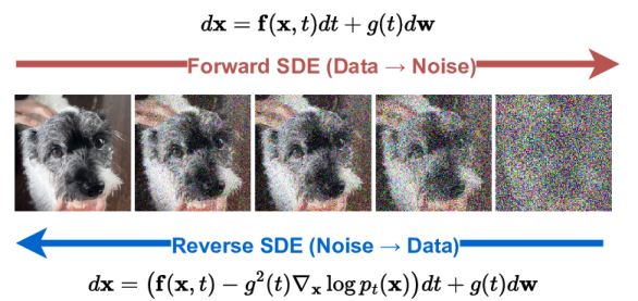
Figure 2. The overall framework of score-based generative models. SGMs corrupt the input data with increasing noise and generate a new sample from the noisy data.

2.2. Score-based Generative Models (SGMs)

Score-based generative models (SGMs) (Song et al., 2021) are a novel generative model paradigm that effectively addresses the challenges of generative models. Fig. 2 introduces the overall framework of SGMs, which utilizes a stochastic differential equation (SDE) to model the forward and reverse processes. The forward process involves adding noise to the initial input data, while the reverse process is to remove noises from the noisy data to generate a new sample.

SGMs define the forward SDE with the following Itô SDE:

(4) $$d\mathbf{x}=\mathbf{f}(\mathbf{x},t)dt+g(t)d\mathbf{w},$$

where $\mathbf{f}(\mathbf{x},t)=f(t)\mathbf{x}$ and its reverse SDE is defined as follows:

(5) $$d\mathbf{x}=\big{(}\mathbf{f}(\mathbf{x},t)-g^{2}(t)\nabla_{\mathbf{x}}\log p_{t}(\mathbf{x})\big{)}dt+g(t)d\mathbf{w},$$

which is a generative process. The function $f$ and $g$ are drift and diffusion coefficients, and $w$ is the standard Wiener process. According to the types of $f$ and $g$, SGMs are classified as i) variance exploding (VE), ii) variance preserving (VP), and ii) sub-variance preserving (Sub-VP) models. In our experiments, we only use VE SDE with the following $f$ and $g$:

(6) $$f(t)=0,\quad g(t)=\sqrt{\frac{d[\sigma^{2}(t)]}{dt}},$$

where the noise scales $\sigma(t)=\sigma_{\text{min}}\Big{(}\frac{\sigma_{\text{max}}}{\sigma_{\text{min}}}\Big{)}^{t}$.

During the forward process, the score function $\nabla_{\mathbf{x}}\log p_{t}(\mathbf{x})$ is approximated by a score network $S_{\phi}(\mathbf{x}(t),t)$. Since the perturbation kernel $p(\mathbf{x}(t)|\mathbf{x}(0))$ can be easily collected, it allows us to calculate the gradient of the log transition probability $\nabla_{\mathbf{x}(t)}\log p(\mathbf{x}(t)|\mathbf{x}(0))$. Therefore, we can easily train a score network $S_{\phi}(\mathbf{x}(t),t)$ as follows:

(7) $$\operatorname*{arg\,min}_{\phi}\mathbb{E}_{t}\mathbb{E}_{\mathbf{x}(t)}\mathbb{E}_{\mathbf{x}(0)}\Big{[}\lambda(t)\big{\|}S_{\phi}(\mathbf{x}(t),t)-\nabla_{\mathbf{x}(t)}\log p(\mathbf{x}(t)|\mathbf{x}(0))\big{\|}_{2}^{2}\Big{]},$$

where $\lambda(t)$ is to control the trade-off between synthesis quality and likelihood. After training the score network, we can generate fake samples using only the reverse SDE.

3. Existing approaches and limitations

3.1. Contrastive Learning for Recommendation

In recent years, deep learning-based recommender systems have been proposed with promising performance. However, they involve obtaining meaningful representations from labeled interaction data, challenges such as data sparsity and cold-start problems can arise. To address these challenges, recommender systems with self-supervised learning (SSL) have emerged, which augment various views and contrast them to align node representations. These approaches can extract meaningful information from unlabeled interactive data and have shown outperforming results in recommender systems (Wu et al., 2021; Yu et al., 2022b, a; Lin et al., 2022; Jing et al., 2023).

SGL (Wu et al., 2021) is the first method applying CL to graph-based collaborative filtering recommendation. It augments the user-item bipartite graph with structure perturbations using three operators: node dropouts, edge dropouts, and random walks. They encode augmented views with the backbone LightGCN, and contrast them with InfoNCE loss (Oord et al., 2018) defined as follows:

(8) $$\mathcal{L}_{CL}:=\sum_{i\in\mathcal{B}}-\log\frac{\exp(\text{sim}(\mathbf{e}_{i}^{\prime},\mathbf{e}_{i}^{\prime\prime})/\tau)}{\sum_{j\in\mathcal{B}}\exp(\text{sim}(\mathbf{e}_{i}^{\prime}\mathbf{e}_{j}^{\prime\prime})/\tau)},$$

where $i$, $j$ are a user and an item in a mini-batch $\mathcal{B}$ respectively, $\text{sim}(\cdot)$ is the cosine similarity, $\tau$ is the temperature, and $\mathbf{e}^{\prime}$, $\mathbf{e}^{\prime\prime}$ are $L_{2}$-normalized augmented node representations. The CL loss increases the alignment between the node representations of $\mathbf{e}_{i}^{\prime}$ and $\mathbf{e}_{i}^{\prime\prime}$ nodes, viewing the representations of the same node $i$ as positive pairs. Simultaneously, it minimizes the alignment between the node representations of $\mathbf{e}_{i}^{\prime}$ and $\mathbf{e}_{j}^{\prime\prime}$, viewing the representations of the different nodes $i$ and $j$ as negative pairs. However, it can result in a potential loss of detailed interaction information and topology although successful.

NCL (Lin et al., 2022) is a model which proposes a prototypical contrastive objective to capture the correlations between a user/item and its context. It explicitly integrates the potential neighbors from graph structure and semantic space, respectively, into contrastive pairs.

SimGCL (Yu et al., 2022b) pointed out that the graph augmentation method of SGL causes information loss and also plays only a trivial role in CL. To generate contrastive views, it discards the graph augmentation and simply adds the same scale uniform noise to the embedding space, and outperforms previous CL-based methods. However, SimGCL compromises the unique characteristics of each node on a graph by adding noises with the same scale.

3.2. Negative Sampling Problem

For graph-based CF models with implicit feedback, the negative sampling problem refers to the challenge encountered when training only with observed interactions. In most cases, user interactions such as purchasing products or clicking on items are considered positive signals, however, it can lead to difficulties when trying to predict unobserved interactions. Therefore, various negative sampling techniques have been explored to select proper negative signals from unobserved interactions. These approaches have yielded significant success in enhancing the accuracy and diversity of recommendation systems (Zhang et al., 2013; Huang et al., 2021; Ding et al., 2020; Rendle and Freudenthaler, 2014; Huang et al., 2020; Wu et al., 2023b).

A crucial aspect of negative sampling is defining hard negative samples to learn the boundary between positive and negative items. DNS (Zhang et al., 2013) is a dynamic negative sampling strategy by selecting the negative item with the highest score by the recommender. IRGAN (Wang et al., 2017), which is a GAN-based model, generates hard negative samples that confuse the recommender. MixGCF (Huang et al., 2021) is the state-of-the-art negative sampling method, which adopts positive mixing and hop mixing. In positive mixing, it utilizes the interpolation method by injecting positive information, and in hop mixing, it aggregates negative samples from selected hops of their neighbors. However, DNS and MixGCF are simplistic approaches for synthesizing hard negative samples only in a predetermined region, which can lead to a limited diversity in them.

4. Proposed Methods

In this section, we first outline the three design goals of our proposed method. These goals serve as guiding principles throughout the development of our model. The goals are as follows:

1. Personalization. We need to design a user-item specific sampling method for personalized recommendations.

2. Robustness. Our method should have high robustness even under user sparsity and item popularity.

3. Diversity. Our method should consider not only the accuracy of recommendations but also the improvement of diversity.

With these goals as a design philosophy, we then delve into the overall architecture of our SCONE model, detailing each component and its contribution. Subsequently, a comprehensive comparison with existing recommendation methods is presented, highlighting SCONE’s unique approach and advantages.

4.1. Overall Model Architecture

In Fig. LABEL:fig:method_1, we show the overall model architecture of SCONE. Following existing graph-based CF models, i.e., SGL, SimGCL, and MixGCF, we adopt a simple but effective model LightGCN as our graph encoder. Given the initial user and item embeddings $\Theta=\mathbf{E}^{(0)}$, LightGCN learns these embeddings by performing a linear propagation on the user-item interaction graph. After that, we train a score-based generative model using the final embeddings $\mathbf{E}$, which is the weighted sum of the embeddings learned at all layers of LightGCN. The score function $\nabla_{\mathbf{e}}\log p_{t}(\mathbf{e})$ is approximated by a score network. The trained SGM is used in two ways: i) contrastive views generation for CL and ii) hard negative samples generation. Further details will be described in Sections 4.3 and 4.4, respectively.

We design our score network modified from U-Net (Ronneberger et al., 2015). We use 3 layers, 1 encoding block, and 1 decoding block linked by skip connection. The network architecture $S_{\phi}(\mathbf{e}(t),t)$ is as follows:

(9) $$h_{0}=\mathtt{FC}_{0}(\mathbf{e}(t)),$$

$$h_{1}=\mathtt{FC}_{1}^{2}(\mathtt{tanh}(\mathtt{FC}_{1}^{1}(h_{0}))\oplus\mathtt{FC}_{1}^{t}(t_{\text{emb}})),$$

$$h_{2}=\mathtt{tanh}(\mathtt{FC}_{2}(h_{1})),$$

$$h_{3}=\mathtt{FC}_{3}^{2}(\mathtt{tanh}(\mathtt{FC}_{3}^{1}(h_{2}\odot h_{1}))\oplus\mathtt{FC}_{3}^{t}(t_{\text{emb}})),$$

$$S_{\phi}(\mathbf{e}(t),t)=\mathtt{FC}_{4}(h_{3}),$$

where $\mathtt{FC}$ is a fully connected layer, $\odot$ is the concatenation operator, $h_{i}$ is the $i^{th}$ hidden vector, and $\oplus$ is the element-wise addition. The encoding and decoding blocks are symmetric, where $\text{dim}(h_{0})=\text{dim}(h_{3})$ and $\text{dim}(h_{1})=\text{dim}(h_{2})$, and the output of model has the same dimensionality $D$ as input $\mathbf{e}$. The time embedding $t_{emb}$ is defined as follows:

(10) $$t_{\text{emb}}=\mathtt{FC}_{\text{emb}}^{2}(\mathtt{tanh}(\mathtt{FC}_{\text{emb}}^{1}(\mathtt{Emb}(t)))),$$

where $\mathtt{Emb}$ is a sinusoidal positional embedding (Vaswani et al., 2017).

0:  $N$: Number of sampling steps for the reverse process

1:  $\mathbf{e}(N)\sim\mathcal{N}\big{(}\mathbf{e}(0),[\sigma^{2}(N)-\sigma^{2}(0)]\mathbf{I}\big{)}$

2:  for $i=N-1$ to $0$ do

3:     $\mathbf{e}(i)\leftarrow\mathbf{e}(i+1)+\big{(}\sigma^{2}(i+1)-\sigma^{2}(i)\big{)}\cdot S_{\phi}\big{(}\mathbf{e}(i+1),\sigma(i+1)\big{)}$

4:     $z\sim\mathcal{N}(\mathbf{0},\mathbf{I})$

5:     $\mathbf{e}(i)\leftarrow\mathbf{e}(i)+\sqrt{\sigma^{2}(i+1)-\sigma^{2}(i)}\cdot z$

6:  end for

7:  return  $\mathbf{e}(N)$ and $\hat{\mathbf{e}}(0)$

Algorithm 1 Contrastive views generation

0:  $N$: Number of sampling steps for the reverse process

1:  $\mathbf{e}_{v^{-}}^{hard}(N)\sim\mathcal{N}\big{(}\mathbf{e}_{v^{-}}(0),[\sigma^{2}(N)-\sigma^{2}(0)]\mathbf{I}\big{)}$

2:  $\mathbf{e}_{v^{+}}(N)\sim\mathcal{N}\big{(}\mathbf{e}_{v^{+}}(0),[\sigma^{2}(N)-\sigma^{2}(0)]\mathbf{I}\big{)}$

13:  for $i=N-1$ to $0$ do

4:     $\mathbf{e}_{v^{-}}^{hard}(i+1)=w\cdot\mathbf{e}_{v^{-}}^{hard}(i+1)+(1-w)\cdot\mathbf{e}_{v^{+}}(i+1)$

5:     $\mathbf{e}(i+1)\leftarrow\mathrm{CONCAT}\big{(}\mathbf{e}_{v^{-}}^{hard}(i+1),\mathbf{e}_{v^{+}}(i+1)\big{)}$

6:     $\mathbf{e}(i)\leftarrow\mathbf{e}(i+1)+\big{(}\sigma^{2}(i+1)-\sigma^{2}(i)\big{)}\cdot S_{\phi}\big{(}\mathbf{e}(i+1),\sigma(i+1)\big{)}$

7:     $z\sim\mathcal{N}(\mathbf{0},\mathbf{I})$

8:     $\mathbf{e}(i)\leftarrow\mathbf{e}(i)+\sqrt{\sigma^{2}(i+1)-\sigma^{2}(i)}\cdot z$

9:     Split $\mathbf{e}(i)$ into two vectors $\mathbf{e}_{v^{-}}^{hard}(i)$ and $\mathbf{e}_{v^{+}}(i)$.

10:  end for

11:  return  $\hat{\mathbf{e}}_{v^{-}}^{hard}(0)$

Algorithm 2 Hard negative samples generation

4.2. User-Item Specific Stochastic Sampling

Generating contrastive views and hard negative samples needs user-item specific sampling schemes for personalized recommendations. It is not feasible to directly apply the denoising process of the diffusion model, which generates a new sample $\hat{\mathbf{x}}(0)$ from a noisy sample $\mathbf{x}(T)$, because it cannot maintain the specific characteristics of users and items. Therefore, we devise a user-item specific sampling scheme for personalized recommendation.

As shown in Figs. LABEL:fig:method_2 and LABEL:fig:method_3, instead of synthesizing $\hat{\mathbf{e}}(0)$ from the entire noise space, we perturb the final embedding $\mathbf{e}(0)$ to an intermediate time $t=N$, and then generate a sample $\hat{\mathbf{e}}(0)$ from an intermediate noisy sample $\mathbf{e}(N)$ using the reverse process of the SGM. It allows the generated embedding to retain specific characteristics of the user or item. This approach is applicable to contrastive views and hard negative samples generation. We set the intermediate time $N=10$ in our experiments, and the impact of the number of sampling steps $N$ is presented in Section 5.5.

4.3. Contrastive Views Generation via a Stochastic Process

As shown in Fig. LABEL:fig:method_2, we define two contrastive views for CL with the SGM as follows:

(11) $$\mathbf{e}^{\prime}=\mathbf{e}(N),\quad\mathbf{e}^{\prime\prime}=\hat{\mathbf{e}}(0),$$

where the first view $\mathbf{e}^{\prime}$ is a perturbed embedding $\mathbf{e}(N)$ using the forward process with Eq. (4), and the second view $\mathbf{e}^{\prime\prime}$ is a generated embedding $\hat{\mathbf{e}}(0)$ from $\mathbf{e}(N)$ using the reverse process with Eq. (5). The detailed stochastic sampling process for the generation of contrastive views is in Alg. 1. We sample an intermediate noisy vector $\mathbf{e}(N)$ with the forward process and convert it into a synthesized sample $\hat{\mathbf{e}}(0)$ through $N$ steps. The stochastic process of the SGM leads not converge to the original but to another sample.

4.4. Hard Negative Samples Generation via a Stochastic Positive Injection

To enhance the learning of the boundary between positive and negative samples, we propose a stochastic positive injection method to generate hard negative samples close to positive samples. Fig. LABEL:fig:method_3 shows the process of generating hard negative samples. Firstly, we use the random sampling method in the BPR loss, where positive and negative samples are sampled from a uniform distribution. After sampling a triplet input $(u,v^{+},v^{-})$, we sample intermediate noisy vectors $\mathbf{e}_{v^{-}}^{hard}(N)$ and $\mathbf{e}_{v^{+}}(N)$ with the forward process. Then, positive samples are continuously injected into negative samples during the stochastic sampling process of SGM. The stochastic positive injection is defined as follows:

(12) $$\mathbf{e}_{v^{-}}^{hard}(t)=w\cdot\mathbf{e}_{v^{-}}^{hard}(t)+(1-w)\cdot\mathbf{e}_{v^{+}}(t)$$

where $w$ is hyperparameters to regulate the weight of stochastic positive injection. Alg. 2 shows the detailed hard negative samples generation process. We define a hard negative sample $\mathbf{e}_{v^{-}}^{hard}(t)$ by injecting a positive sample $\mathbf{e}_{v^{+}}(t)$ for $N$ steps, and finally, we generate a hard negative sample $\hat{\mathbf{e}}_{v^{-}}^{hard}(0)$. These synthesized samples cover the entire embedding region rather than a predefined point.

0:  Training set $\{(u,v^{+},v^{-})\}$, Graph encoder $f(\cdot)$, Score network $S(\cdot)$

1:  Initialize $\Theta$ and $\phi$

2:  while not converged do

3:     Sample a batch of user-item pairs $(u,v^{+},v^{-})$.

4:     Get the user and item embeddings by encoder $f(\cdot)$.

5:     Generate augmented views $\mathbf{e}^{\prime}$ and $\mathbf{e}^{\prime\prime}$ by Alg. 1.

6:     Generate a hard negative sample $\hat{\mathbf{e}}_{v^{-}}^{hard}(0)$ by Alg. 2.

7:     Calculate $\mathcal{L}_{\Theta}$ with $\mathcal{L}_{BPR}$ and $\mathcal{L}_{CL}$ by Eq. (13).

8:     Calculate $\mathcal{L}_{\phi}$ with Eq. (14).

9:     Update $\Theta$ and $\phi$.

10:  end while

11:  return  $\Theta$ and $\phi$

Algorithm 3 The training algorithm of SCONE

4.5. Training Algorithm

The training algorithm of SCONE is in Alg. 3. The model parameters $\Theta$ of the graph encoder and $\phi$ of SGM are jointly trained end-to-end. The graph encoder is optimized through the sum of the BPR and CL losses, and SGM is trained with denoising score matching loss. SGM generates contrastive views for CL and hard negative samples, which are employed when optimizing $\Theta$. The objective functions for approximating $\Theta$ and $\phi$ are as follows:

(13) $$\mathcal{L}_{\Theta} =\mathcal{L}_{BPR}+\lambda_{1}\mathcal{L}_{CL},$$

(14) $$\mathcal{L}_{\phi} =\mathbb{E}_{t}\mathbb{E}_{\mathbf{e}(t)}\mathbb{E}_{\mathbf{e}(0)}\Big{[}\lambda(t)\|S_{\phi}(\mathbf{e}(t),t)-\nabla_{\mathbf{e}(t)}\log p(\mathbf{e}(t)|\mathbf{e}(0))\|_{2}^{2}\Big{]},$$

where $\lambda_{1}$ is hyperparameters to control the strengths of CL. For contrastive learning, we adopt CL loss as InfoNCE (Oord et al., 2018), following the approach of SGL and SimGCL. $\mathcal{L}_{BPR}$ and $\mathcal{L}_{CL}$ are as follows:

(15) $$\mathcal{L}_{BPR}=\sum_{(u,v^{+},v^{-})\in\mathcal{O}}{\ln{\sigma(\mathbf{e}_{u}\cdot\hat{\mathbf{e}}_{v^{-}}^{hard}(0)-\mathbf{e}_{u}\cdot\mathbf{e}_{v^{+}})}}+\lambda_{2}\|\Theta\|_{2}^{2},$$

(16) $$\mathcal{L}_{CL}=\sum_{i\in\mathcal{B}}-\log\frac{\exp(\text{sim}(\mathbf{e}_{i}^{\prime},\mathbf{e}_{i}^{\prime\prime})/\tau)}{\sum_{j\in\mathcal{B}}\exp(\text{sim}(\mathbf{e}_{i}^{\prime},\mathbf{e}_{j}^{\prime\prime})/\tau)},$$

where $\hat{\mathbf{e}}_{v^{-}}^{hard}(0)$ is a generated hard negative sample by SGM (cf. Line 6 of Alg. 3), and $\mathbf{e}^{\prime}$ and $\mathbf{e}^{\prime\prime}$ are contrastive views with the stochastic process of SGM (cf. Line 5 of Alg. 3).

Table 2. Comparison of existing methods that focuses on i) how to generate contrastive views for CL and ii) how to define negative samples

Model	Contrastive Views	Negative Samples
LightGCN (He et al., 2020)	✗	Random sampling
SGL (Wu et al., 2021)	Perturbing graph structure	Random sampling
SimGCL (Yu et al., 2022b)	Injecting noises into embeddings	Random sampling
DNS (Zhang et al., 2013)	✗	Promising candidate
MixGCF (Huang et al., 2021)	✗	Linear interpolation
SCONE	Stochastic sampling with SGMs

4.6. Discussion: Relation to Other Methods

Table 2 presents a comparison of existing approaches that focus on generating contrastive views and negative samples. In this section, we compare our method with existing methods in terms of pros and cons, and space and time complexity.

4.6.1. Contrastive views

Diverse users and items exhibit distinctive characteristics, and view generation techniques should be customized for each user. SCONE generates contrastive views using a stochastic process with score-based generative models. It is capable of approximating data distributions without information distortion. In particular, it can sample with high diversity while preserving specific characteristics of each node for personalized recommendations due to the user-item specific stochastic sampling. However, SGL and SimGCL are exposed to information distortions. SGL perturbs the inherent characteristic of the graph through edge/node dropouts. In addition, SimGCL undermines the individual characteristic of each node by adding noises.

4.6.2. Negative sampling

SCONE generates hard negative samples with a stochastic positive injection. It can cover the entire embedding region rather than a predetermined space. However, LightGCN, SGL, and SimGCL adopt a random negative sampling (RNS) method, which randomly selects unobserved interaction signals. This approach often fails to capture the popularity of the item. Furthermore, DNS and MixGCF confine the selection of negative samples into a limited space. For DNS, promising candidate items are predefined in a discrete space, and for MixGCF, the sampled hard negative sample is a linear interpolation between the positive and negative items.

4.6.3. Space and time complexity

Regarding the model parameters, LightGCN, SGL, SimGCL, DNS, and MixGCF only require initial embeddings $\Theta=\mathbf{E}$, whereas SCONE needs the additional parameters $\phi$ for the score network. However, the number of the parameters $\Theta$ is 9 times larger than that of $\phi$ in Douban, and 24 times in Tmall. Therefore, it does not significantly increase the space complexity.

In terms of the time complexity, both SGL and SimGCL require three iterations of graph convolution networks to generate the final embeddings for recommendation and two augmented embeddings for CL. In contrast, DNS and MixGCF need only one iteration. However, they need considerable time to define hard negative samples. For DNS, it should sort the highest negative items after referring to the currently trained recommendation model during training and for MixGCF, it uses a positive and hop mixing module by the linear combination and hop-grained scheme. Our SCONE also requires only one iteration of graph convolution networks. However, SCONE incurs additional time overheads for generating contrastive views and hard negative samples. Although generating samples through SGMs typically takes a long time for images, SCONE can reduce the sampling time by decreasing the number of steps, $N$. In Sec. 5.6, we compare the training time. SCONE takes a longer time compared to graph-based CL methods, but is faster than negative sampling methods.

Table 3. Statistics of the datasets

Dataset	#Users	#Items	#Interactions	Density
Douban	12,638	22,222	598,420	0.213%
Gowalla	50,821	57,440	1,302,695	0.045%
Tmall	47,939	41,390	2,619,389	0.132%
Yelp2018	31,668	38,048	1,561,406	0.130%
Amazon-CDs	43,169	35,648	777,426	0.051%
ML-1M	6,038	3,492	575,281	2.728%

Table 4. Performance comparison with state-of-the-art models. The best results are highlighted in bold face, and the second best results are with underline.

Dataset	Metric	GCN-based		Contrastive Learning				Negative Sampling			SCONE	Imp.
		LightGCN		SGL	NCL	SimGCL		DNS	MixGCF
Douban	Recall@20	0.1474		0.1728	0.1638	0.1780		0.1645	0.1784		0.1815	1.70%
	NDCG@20	0.1240		0.1510	0.1403	0.1567		0.1393	0.1576		0.1611	2.79%
Gowalla	Recall@20	0.2086		0.2223	0.2235	0.2269		0.2233	0.2147		0.2295	1.15%
	NDCG@20	0.1264		0.1349	0.1353	0.1386		0.1358	0.1295		0.1409	1.66%
Tmall	Recall@20	0.0686		0.0754	0.0700	0.0898		0.0860	0.0819		0.0908	1.08%
	NDCG@20	0.0477		0.0532	0.0492	0.0643		0.0600	0.0570		0.0654	1.73%
Yelp2018	Recall@20	0.0588		0.0669	0.0654	0.0718		0.0671	0.0703		0.0721	0.39%
	NDCG@20	0.0485		0.0552	0.0540	0.0593		0.0551	0.0576		0.0594	0.27%
Amazon-CDs	Recall@20	0.1283		0.1550	0.1483	0.1584		0.1545	0.1542		0.1586	0.13%
	NDCG@20	0.0779		0.0986	0.0940	0.1006		0.0972	0.0960		0.1009	0.30%
ML-1M	Recall@20	0.2693		0.2657	0.2777	0.2868		0.2791	0.2897		0.2910	0.45%
	NDCG@20	0.3015		0.3027	0.3150	0.3230		0.3171	0.3287		0.3244	-1.31%

5. Experiments

In this section, we introduce our extensive experimental results. To demonstrate the superiority of SCONE and clarify its effectiveness, we answer the following research questions:

• RQ1: How does SCONE perform as compared with various state-of-the-art models?

• RQ2: Is the robustness of SCONE, with respect to user sparsity and item popularity, superior to the baselines?

• RQ3: Do all proposed methods improve the effectiveness?

• RQ4: What is the influence of different settings on SCONE?

5.1. Experimental Settings

5.1.1. Datasets and Evaluation Metrics

We conduct experiments on 6 benchmark datasets: Douban, Gowalla, Tmall, Yelp2018, Amazon-CDs, and ML-1M (Yu et al., 2021; He et al., 2020; Cai et al., 2023; Harper and Konstan, 2015; Yu et al., 2022b). We summarize the statistics of the datasets in Table 3. We follow the same strategy described in (Yu et al., 2022b) to split the datasets into training, validation, and testing set with a ratio of 7:1:2. We adopt widely-used Recall@20 and NDCG@20 to evaluate the performance of the top-K recommendation.

5.1.2. Baselines

We choose LightGCN as the backbone model, and compare SCONE with the following 6 baselines:

• Graph-based methods: LightGCN (He et al., 2020);

• Graph-based CL methods: SGL (Wu et al., 2021), NCL (Lin et al., 2022), SimGCL (Yu et al., 2022b);

• Negative sampling methods: DNS (Zhang et al., 2013), MixGCF (Huang et al., 2021).

5.1.3. Hyperparameters

To make a fair comparison with previous studies, we follow hyperparameters settings in the original papers. For all the models, the embedding size $D$ is set as 64, the batch size is 2048, and we use $L=2$ for the graph encoder. For our model, we use only VE SDE, and the learning rate is 0.001. We set $\sigma_{\text{min}}=0.01$, $\sigma_{\text{max}}=50$, $T=100$, $N=10$, $\tau=0.2$, $\lambda_{2}=10^{-4}$, $\text{dim}(h_{0})=64$, and $\text{dim}(h_{1})=128$. We tune $\lambda_{1}$ within the ranges of $\{0.1,0.2,0.5,0.7,0.9,1.0,2.0,2.5\}$, and $w$ is searched from $\{0.7,0.8,0.9\}$. The best hyperparameters in each dataset are as follows: In douban, $\lambda_{1}=0.5$ and $w=0.9$. In Gowalla, $\lambda_{1}=0.9$ and $w=0.7$. In Tmall, $\lambda_{1}=2.5$ and $w=0.9$. In Yelp2018, $\lambda_{1}=0.7$ and $w=0.7$. In Amazon-CDs, $\lambda_{1}=0.2$ and $w=0.8$. In ML-1M, $\lambda_{1}=0.1$ and $w=0.8$.

5.1.4. Experimental environments

Our software and hardware environments are as follows: Ubuntu 18.04.6 LTS, Python 3.10.8, Pytorch 1.11.0, CUDA 11.7, and NVIDIA Driver 470.161.03, i9, CPU, and NVIDIA RTX 3090.

5.2. Performance Comparison with SOTA (RQ1)

As shown in Table 4, we summarize the overall performance of 6 baselines on the 6 datasets in terms of Recall@20 and NDCG@20. We find the following observations:

1. In most cases, graph-based CL and negative sampling methods are effective in enhancing the performance of LightGCN. It indicates that both two approaches are valid for improving recommendation performance. Specifically, SimGCL and MixGCF outperform LightGCN by large margins in Tmall and Douban, which improves NDCG@20 by 34.88% and 27.07%, respectively.

2. In graph-based CL models, SimGCL is the most effective model, and even compared to Negative sampling methods, it ranks the second best in 4 out of 6 datasets. In particular, SimGCL demonstrates remarkable performance improvements on sparser datasets such as Gowalla and Amazon-CDs, indicating that CL alleviates the challenge of data sparsity.

3. In negative sampling methods, DNS and MixGCF are hard to determine superiority. The performance of MixGCF is better than DNS in denser datasets, while worse in the sparser datasets.

4. SCONE achieves the best performance in almost all cases, which proves the effectiveness of our proposed methods. By generating various augmented views and hard negative samples with stochastic sampling, SCONE not only mitigates the data sparsity problem but also improves the generalization of the model.

5.3. Robustness of SCONE (RQ2)

5.3.1. User sparsity

To evaluate the ability to alleviate user sparsity, we categorize users into three subsets by their interaction degree: the lowest 80% users with the fewest number of interactions, the range from the bottom 80% to 95%, and the top 5%. As shown in Fig. LABEL:fig:exp_user, SCONE consistently outperforms the other baselines in almost all groups. Especially, SCONE shows good performance for extremely sparse user groups in all datasets.

5.3.2. Item popularity

Similar to user sparsity analysis, we categorize items into three groups based on item popularity. We calculate the Recall@20 value that each group contributes, which is called decomposed Recall@20. The total Recall@20 value is equal to the sum of the values from the three groups. In Fig. LABEL:fig:exp_item, our model shows performance improvement over other baselines in an item group with low popularity, demonstrating robustness to item popularity.

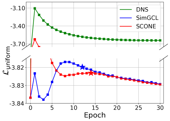
Figure 9. The uniformity curves in the dataset of Tmall. The star denotes the epoch at the best performance.

5.3.3. Uniformity

In this section, we measure the uniformity of the representation, which is the logarithm of the average pairwise Gaussian potential (Wang and Isola, 2020):

(17) $$\mathcal{L}_{\text{uniform}}=\log\underset{\begin{subarray}{c}i.i.d\\ u,v\sim p_{\text{node}}\end{subarray}}{\mathbb{E}}e^{-2\|g(u)-g(v)\|_{2}^{2}}.$$

where $g(\cdot)$ is the normalized embedding. In Douban and Tmall datasets, we randomly sample 5,000 users and the popular items with more than 200 interactions. After that, we compute the uniformity of their representations in SCONE and baselines with Eq. (17). As shown in Fig. 9, all uniformity curves show similar trends. In the early steps of training, it has a high uniformity value and then decreases, and after reaching the peak, it tends to gradually converge. In Table 5, our method shows the highest uniformity at the best performance compared with the other baselines. When considered in conjunction with the results in Fig. LABEL:fig:exp_item, these findings suggest that our approach not only mitigates popularity bias but also enhances the diversity and personalization of user recommendations.

Table 5. The uniformity at the best performance. The lower values have higher uniformity.

Model	Douban	Tmall
LightGCN	-2.317	-3.142
SGL	-3.474	-3.723
SimGCL	-3.469	-3.820
DNS	-2.639	-3.642
MixGCF	-3.107	-3.536
SCONE	-3.591	-3.823

5.4. Ablation Study of SCONE (RQ3)

As shown in Fig. LABEL:fig:exp_ablation, we conduct ablation experiments to the efficacy of the contrastive learning and negative sampling on SCONE. ‘LightGCN’ means the model trained without CL and hard negative sampling, ‘w/o NS’ means without hard negative sampling but with only CL, and ‘w/o CL’ means without CL with only hard negative sampling. In all datasets, our contrastive learning and hard negative sampling methods significantly improve recommendation performance. Especially, in Figs. LABEL:fig:exp_ablation(b) and LABEL:fig:exp_ablation(d), we demonstrate the effectiveness of our proposed methods by a large margin.

5.5. Sensitivity Studies (RQ4)

In this section, we study the impact of the three key hyperparameters: the regularization weight $\lambda_{1}$ of CL, the weight $w$ of stochastic positive injection, and the number of sampling steps $N$.

5.5.1. The regularization weight $\lambda_{1}$ of contrastive learning

We conduct experiments by changing the value of $\lambda_{1}$ as shown in Fig. LABEL:fig:exp_lambda. In Amazon-CDs and ML-1M, SCONE achieves the best performance when $\lambda_{1}=0.2$ and $\lambda_{1}=0.1$, respectively. In both datasets, as the value of $\lambda_{1}$ increases, the performance decreases.

5.5.2. The weight $w$ of stochastic positive injection

We think that the smaller value of $w$ leads to lower performance due to the large injection of positive information. In Fig. LABEL:fig:exp_w, when $w$ is lower than 0.7, SCONE shows a dramatic change in the performance. It can be seen that it is helpful to inject only a certain amount of positive information while maintaining the nature of the negative samples.

5.5.3. The number of sampling steps $N$ in stochastic sampling

For personalized recommendation, we perturb the final embeddings to the intermediate time $N$ and generate contrastive views and hard negative samples from the intermediate noisy sample. As shown in Fig. LABEL:fig:exp_N, when $N$ is larger than 10, the model performance is degraded since augmented views and hard negative samples are generated after perturbing through many time steps. In SCONE, it is important to retain specific characteristics of users and items, therefore, we set $N=10$ in our all experiments.

5.6. Runtime Analyses

In Table 6, we report the running time for one epoch during training. Based on the number of interactions among the 6 datasets used in our experiments, we measure the running time with Douban, which has a small number of interactions, Yelp2018 with the intermediate interactions, and Tmall with the largest number of interactions.

For SGL and SimGCL, additional computation for the graph convolution is required when compared with LightGCN. Likewise, DNS and MixGCF need to computation of the negative sampling process. Due to the computationally expensive nature of stochastic sampling in diffusion models, SCONE takes longer than graph-based CL methods, but our method has better performance. Compared with existing negative sampling methods, SCONE is faster and shows better performance. All baselines and SCONE have the same inference time because it is the computation time of the final embedding with the graph encoder.

Table 6. Running time for one epoch

Method	Douban	Tmall	Yelp2018
LightGCN	3.62s	47.81s	15.34s
SGL	8.67s	122.30s	37.41s
SimGCL	8.72s	132.82s	40.04s
DNS	25.23s	154.18s	71.57s
MixGCF	23.25s	163.78s	71.29s
SCONE	19.86s	142.65s	60.63s

6. Conclusion

In this research, we introduced SCONE, a novel framework targeting the challenges of data sparsity and negative sampling in graph-based CF models. The innovative approach of SCONE involves synthesizing samples using a stochastic sampling process, a first in recommender systems, to generate both user-item-specific views and hard negative samples. Our experiments across 6 benchmark datasets show the superiority of SCONE over 6 baselines, demonstrating its efficacy in contrastive learning and negative sampling. The robustness of SCONE in handling user sparsity and item popularity issues underscores its potential as a valuable tool for enhancing recommender systems.

References

- (1)
- Bayer et al. (2017) Immanuel Bayer, Xiangnan He, Bhargav Kanagal, and Steffen Rendle. 2017. A generic coordinate descent framework for learning from implicit feedback. In TheWebConf (former WWW). 1341–1350.
- Cai et al. (2023) Xuheng Cai, Chao Huang, Lianghao Xia, and Xubin Ren. 2023. LightGCL: Simple Yet Effective Graph Contrastive Learning for Recommendation. In ICLR.
- Chen et al. (2020) Lei Chen, Le Wu, Richang Hong, Kun Zhang, and Meng Wang. 2020. Revisiting Graph Based Collaborative Filtering: A Linear Residual Graph Convolutional Network Approach. In AAAI.
- Choi et al. (2023a) Jeongwhan Choi, Seoyoung Hong, Noseong Park, and Sung-Bae Cho. 2023a. Blurring-Sharpening Process Models for Collaborative Filtering. In SIGIR.
- Choi et al. (2021) Jeongwhan Choi, Jinsung Jeon, and Noseong Park. 2021. LT-OCF: Learnable-Time ODE-based Collaborative Filtering. In CIKM.
- Choi et al. (2023b) Jeongwhan Choi, Hyowon Wi, Chaejeong Lee, Sung-Bae Cho, Dongha Lee, and Noseong Park. 2023b. RDGCL: Reaction-Diffusion Graph Contrastive Learning for Recommendation. arXiv preprint arXiv:2312.16563 (2023).
- Covington et al. (2016) Paul Covington, Jay Adams, and Emre Sargin. 2016. Deep Neural Networks for YouTube Recommendations. In Proceedings of the 10th ACM Conference on Recommender Systems. 191–198.
- Ding et al. (2020) Jingtao Ding, Yuhan Quan, Quanming Yao, Yong Li, and Depeng Jin. 2020. Simplify and robustify negative sampling for implicit collaborative filtering. Advances in Neural Information Processing Systems 33 (2020), 1094–1105.
- Fan et al. (2022) Wenqi Fan, Xiaorui Liu, Wei Jin, Xiangyu Zhao, Jiliang Tang, and Qing Li. 2022. Graph Trend Filtering Networks for Recommendation. In SIGIR. 112–121.
- Harper and Konstan (2015) F Maxwell Harper and Joseph A Konstan. 2015. The movielens datasets: History and context. Acm Transactions on Interactive Intelligent Systems (TIIS) 5, 4 (2015), 1–19.
- He and McAuley (2016) Ruining He and Julian McAuley. 2016. Ups and downs: Modeling the visual evolution of fashion trends with one-class collaborative filtering. In proceedings of the 25th international conference on world wide web. 507–517.
- He et al. (2020) Xiangnan He, Kuan Deng, Xiang Wang, Yan Li, YongDong Zhang, and Meng Wang. 2020. LightGCN: Simplifying and Powering Graph Convolution Network for Recommendation. In SIGIR.
- Hong et al. (2022) Seoyoung Hong, Minju Jo, Seungji Kook, Jaeeun Jung, Hyowon Wi, Noseong Park, and Sung-Bae Cho. 2022. TimeKit: A Time-series Forecasting-based Upgrade Kit for Collaborative Filtering. In 2022 IEEE International Conference on Big Data (Big Data). IEEE, 565–574.
- Hu et al. (2024) Jun Hu, Bryan Hooi, Shengsheng Qian, Quan Fang, and Changsheng Xu. 2024. MGDCF: Distance learning via markov graph diffusion for neural collaborative filtering. IEEE Transactions on Knowledge and Data Engineering (2024).
- Huang et al. (2020) Jui-Ting Huang, Ashish Sharma, Shuying Sun, Li Xia, David Zhang, Philip Pronin, Janani Padmanabhan, Giuseppe Ottaviano, and Linjun Yang. 2020. Embedding-based retrieval in facebook search. In KDD. 2553–2561.
- Huang et al. (2021) Tinglin Huang, Yuxiao Dong, Ming Ding, Zhen Yang, Wenzheng Feng, Xinyu Wang, and Jie Tang. 2021. Mixgcf: An improved training method for graph neural network-based recommender systems. In KDD. 665–674.
- Jiang et al. (2023) Juyong Jiang, Peiyan Zhang, Yingtao Luo, Chaozhuo Li, Jae Boum Kim, Kai Zhang, Senzhang Wang, Xing Xie, and Sunghun Kim. 2023. AdaMCT: adaptive mixture of CNN-transformer for sequential recommendation. In CIKM. 976–986.
- Jing et al. (2023) Mengyuan Jing, Yanmin Zhu, Tianzi Zang, and Ke Wang. 2023. Contrastive Self-supervised Learning in Recommender Systems: A Survey. arXiv preprint arXiv: Arxiv-2303.09902 (2023).
- Kim et al. (2023) Taekyung Kim, Debasmit Das, Seokeon Choi, Minki Jeong, Seunghan Yang, Sungrack Yun, and Changick Kim. 2023. Neural Transformation Network To Generate Diverse Views for Contrastive Learning. In Proceedings of the IEEE/CVF Conference on Computer Vision and Pattern Recognition. 4900–4910.
- Kong et al. (2022) Taeyong Kong, Taeri Kim, Jinsung Jeon, Jeongwhan Choi, Yeon-Chang Lee, Noseong Park, and Sang-Wook Kim. 2022. Linear, or Non-Linear, That is the Question!. In WSDM. 517–525.
- Li et al. (2022) Dongdong Li, Zhigang Wang, Jian Wang, Xinyu Zhang, Errui Ding, Jingdong Wang, and Zhaoxiang Zhang. 2022. Self-Guided Hard Negative Generation for Unsupervised Person Re-Identification. In IJCAI.
- Lim et al. (2022) Hongjun Lim, Yeon-Chang Lee, Jin-Seo Lee, Sanggyu Han, Seunghyeon Kim, Yeongjong Jeong, Changbong Kim, Jaehun Kim, Sunghoon Han, Solbi Choi, et al. 2022. AiRS: a large-scale recommender system at naver news. In ICDE. 3386–3398.
- Lin et al. (2022) Zihan Lin, Changxin Tian, Yupeng Hou, and Wayne Xin Zhao. 2022. Improving graph collaborative filtering with neighborhood-enriched contrastive learning. In Proceedings of the ACM Web Conference 2022. 2320–2329.
- Linden et al. (2003) Greg Linden, Brent Smith, and Jeremy York. 2003. Amazon. com recommendations: Item-to-item collaborative filtering. IEEE Internet computing 7, 1 (2003), 76–80.
- Liu et al. (2021) Fan Liu, Zhiyong Cheng, Lei Zhu, Zan Gao, and Liqiang Nie. 2021. Interest-Aware Message-Passing GCN for Recommendation. In TheWebConf (former WWW). 1296–1305.
- Mao et al. (2021a) Kelong Mao, Jieming Zhu, Jinpeng Wang, Quanyu Dai, Zhenhua Dong, Xi Xiao, and Xiuqiang He. 2021a. SimpleX: A Simple and Strong Baseline for Collaborative Filtering. In CIKM. 1243–1252.
- Mao et al. (2021b) Kelong Mao, Jieming Zhu, Xi Xiao, Biao Lu, Zhaowei Wang, and Xiuqiang He. 2021b. UltraGCN: Ultra Simplification of Graph Convolutional Networks for Recommendation. In CIKM.
- Ni et al. (2023) Yongxin Ni, Yu Cheng, Xiangyan Liu, Junchen Fu, Youhua Li, Xiangnan He, Yongfeng Zhang, and Fajie Yuan. 2023. A Content-Driven Micro-Video Recommendation Dataset at Scale. arXiv preprint arXiv:2309.15379 (2023).
- Oord et al. (2018) Aaron van den Oord, Yazhe Li, and Oriol Vinyals. 2018. Representation learning with contrastive predictive coding. arXiv preprint arXiv:1807.03748 (2018).
- Rendle and Freudenthaler (2014) Steffen Rendle and Christoph Freudenthaler. 2014. Improving pairwise learning for item recommendation from implicit feedback. In WSDM. 273–282.
- Rendle et al. (2009) Steffen Rendle, Christoph Freudenthaler, Zeno Gantner, and Lars Schmidt-Thieme. 2009. BPR: Bayesian Personalized Ranking from Implicit Feedback. In UAI.
- Ronneberger et al. (2015) Olaf Ronneberger, Philipp Fischer, and Thomas Brox. 2015. U-net: Convolutional networks for biomedical image segmentation. In International Conference on Medical image computing and computer-assisted intervention. Springer, 234–241.
- Shen et al. (2021) Yifei Shen, Yongji Wu, Yao Zhang, Caihua Shan, Jun Zhang, B. Khaled Letaief, and Dongsheng Li. 2021. How Powerful is Graph Convolution for Recommendation?. In CIKM.
- Shin et al. (2024) Yehjin Shin, Jeongwhan Choi, Hyowon Wi, and Noseong Park. 2024. An Attentive Inductive Bias for Sequential Recommendation Beyond the Self-Attention. In AAAI, Vol. 38. 8984–8992.
- Song et al. (2021) Yang Song, Jascha Sohl-Dickstein, Diederik P Kingma, Abhishek Kumar, Stefano Ermon, and Ben Poole. 2021. Score-Based Generative Modeling through Stochastic Differential Equations. In ICLR.
- van den Berg et al. (2017) Rianne van den Berg, Thomas N. Kipf, and Max Welling. 2017. Graph Convolutional Matrix Completion. In KDD.
- Vaswani et al. (2017) Ashish Vaswani, Noam Shazeer, Niki Parmar, Jakob Uszkoreit, Llion Jones, Aidan N Gomez, Łukasz Kaiser, and Illia Polosukhin. 2017. Attention is all you need. NeurIPS 30 (2017).
- Wang et al. (2017) Jun Wang, Lantao Yu, Weinan Zhang, Yu Gong, Yinghui Xu, Benyou Wang, Peng Zhang, and Dell Zhang. 2017. IRGAN: A Minimax Game for Unifying Generative and Discriminative Information Retrieval Models. In SIGIR.
- Wang and Isola (2020) Tongzhou Wang and Phillip Isola. 2020. Understanding contrastive representation learning through alignment and uniformity on the hypersphere. In ICML. PMLR, 9929–9939.
- Wang et al. (2021) Weilun Wang, Wengang Zhou, Jianmin Bao, Dong Chen, and Houqiang Li. 2021. Instance-wise hard negative example generation for contrastive learning in unpaired image-to-image translation. In Proceedings of the IEEE/CVF International Conference on Computer Vision. 14020–14029.
- Wang et al. (2019) Xiang Wang, Xiangnan He, Meng Wang, Fuli Feng, and Tat-Seng Chua. 2019. Neural Graph Collaborative Filtering. In SIGIR.
- Wu et al. (2023a) Cheng Wu, Chaokun Wang, Jingcao Xu, Ziyang Liu, Kai Zheng, Xiaowei Wang, Yang Song, and Kun Gai. 2023a. Graph Contrastive Learning with Generative Adversarial Network. In Proceedings of the 29th ACM SIGKDD Conference on Knowledge Discovery and Data Mining. 2721–2730.
- Wu et al. (2019) Chuhan Wu, Fangzhao Wu, Mingxiao An, Jianqiang Huang, Yongfeng Huang, and Xing Xie. 2019. NPA: neural news recommendation with personalized attention. In SIGKDD. 2576–2584.
- Wu et al. (2021) Jiancan Wu, Xiang Wang, Fuli Feng, Xiangnan He, Liang Chen, Jianxun Lian, and Xing Xie. 2021. Self-Supervised Graph Learning for Recommendation. In SIGIR. 726–735.
- Wu et al. (2023b) Xi Wu, Liangwei Yang, Jibing Gong, Chao Zhou, Tianyu Lin, Xiaolong Liu, and Philip S Yu. 2023b. Dimension Independent Mixup for Hard Negative Sample in Collaborative Filtering. arXiv preprint arXiv:2306.15905 (2023).
- Xia et al. (2022) Lianghao Xia, Chao Huang, Yong Xu, Jiashu Zhao, Dawei Yin, and Jimmy Huang. 2022. Hypergraph contrastive collaborative filtering. In SIGIR. 70–79.
- Yang et al. (2023) Yonghui Yang, Zhengwei Wu, Le Wu, Kun Zhang, Richang Hong, Zhiqiang Zhang, Jun Zhou, and Meng Wang. 2023. Generative-Contrastive Graph Learning for Recommendation. In SIGIR.
- Ying et al. (2018) Rex Ying, Ruining He, Kaifeng Chen, Pong Eksombatchai, William L. Hamilton, and Jure Leskovec. 2018. Graph Convolutional Neural Networks for Web-Scale Recommender Systems. In KDD.
- Yu et al. (2022a) Junliang Yu, Xin Xia, Tong Chen, Li zhen Cui, Nguyen Quoc Viet Hung, and H. Yin. 2022a. XSimGCL: Towards Extremely Simple Graph Contrastive Learning for Recommendation. arXiv preprint arXiv:2209.02544 (2022).
- Yu et al. (2021) Junliang Yu, Hongzhi Yin, Min Gao, Xin Xia, Xiangliang Zhang, and Nguyen Quoc Viet Hung. 2021. Socially-aware self-supervised tri-training for recommendation. In KDD. 2084–2092.
- Yu et al. (2022b) Junliang Yu, Hongzhi Yin, Xin Xia, Tong Chen, Lizhen Cui, and Quoc Viet Hung Nguyen. 2022b. Are graph augmentations necessary? simple graph contrastive learning for recommendation. In SIGIR. 1294–1303.
- Zhang et al. (2013) Weinan Zhang, Tianqi Chen, Jun Wang, and Yong Yu. 2013. Optimizing top-n collaborative filtering via dynamic negative item sampling. In SIGIR. 785–788.