An Unstructured Mesh Reaction-Drift-Diffusion Master Equation with Reversible Reactions
Abstract
We develop a convergent reaction-drift-diffusion master equation (CRDDME) to facilitate the study of reaction processes in which spatial transport is influenced by drift due to one-body potential fields within general domain geometries. The generalized CRDDME is obtained through two steps. We first derive an unstructured grid jump process approximation for reversible diffusions, enabling the simulation of drift-diffusion processes where the drift arises due to a conservative field that biases particle motion. Leveraging the Edge-Averaged Finite Element method, our approach preserves detailed balance of drift-diffusion fluxes at equilibrium, and preserves an equilibrium Gibbs-Boltzmann distribution for particles undergoing drift-diffusion on the unstructured mesh. We next formulate a spatially-continuous volume reactivity particle-based reaction-drift-diffusion model for reversible reactions of the form . A finite volume discretization is used to generate jump process approximations to reaction terms in this model. The discretization is developed to ensure the combined reaction-drift-diffusion jump process approximation is consistent with detailed balance of reaction fluxes holding at equilibrium, along with supporting a discrete version of the continuous equilibrium state. The new CRDDME model represents a continuous-time discrete-space jump process approximation to the underlying volume reactivity model. We demonstrate the convergence and accuracy of the new CRDDME through a number of numerical examples, and illustrate its use on an idealized model for membrane protein receptor dynamics in T cell signaling.
I Introduction
Mathematical and computational models have become an invaluable tool in understanding the dynamics of many stochastic cellular processes, governed by a co-action between spatial transport and chemical reactions. Examples of such processes include how ligand binding can affect the functioning of membrane-bound proteins Su et al. (2022); Alberts et al. (2007) and how tethered catalytic reactions control the initiation and integration of T cell activation Zhang et al. (2019). One challenge in developing mathematical models of such processes is that spatial transport of molecules occurs within heterogeneous environments, such as cell membranes, which can significantly impact the dynamics of chemical reaction processes Larsen et al. (2020); Rojas Molina et al. (2021). For example, the geometry of cellular reaction domains can dramatically alter the initial phase of cell polarization Giese et al. (2015), can influence gradient sensing of migratory cells Cheng et al. (2020), and can modulate the propagation of signals from the cell membrane to nucleus Ma et al. (2020).
An additional modeling challenge arises from experimental observations that in many biochemical systems the spatial dynamics of diffusing particles also involves drift. For instance, during T cell synapse formation protein diffusion is influenced by both membrane geometry and the concentration of F-actin fibers near the cell membrane DeMond et al. (2008); Basu and Huse (2017); Siokis et al. (2018). The latter can be modeled as imparting drift due to a conservative force, i.e. potential field, to proteins within the cell membrane. To facilitate the study of reaction-drift-diffusion processes, it is necessary to develop microscopic models and numerical simulation methods that can accurately and explicitly resolve different physical mechanisms modulating the movement of molecules within realistic cellular domains.
In this work, we continue with the setup introduced in Zhang (2015); Isaacson (2013); Isaacson and Zhang (2018) and focus on the spatially continuous volume reactivity (VR) model, modeling particle motion as a drift-diffusion process where the drift is due to a one-body background potential field (i.e. in the absence of reaction, particles move independently with statistics governed by the Fokker-Planck equation). A bimolecular association reaction of the form is modeled through a binding kernel that determines the probability density per time an A molecule at and a B molecule at react and produce a C molecule at inside the domain. We make use of the association kernel to define the unbinding kernel for the backward dissociation reaction, , so that detailed balance of spatial fluxes at equilibrium is preserved. First order reactions of the form are treated as an internal process, with individual particles switching type based on exponential clocks. A special case of the general VR model, for a specific choice of the bimolecular association kernel, is the Doi model Teramoto and Shigesada (1967); Doi (1976a, b).
One common approach for generating approximate realizations of the stochastic process of diffusing and reacting particles is through Brownian Dynamics methods that discretize this process in time Andrews and Bray (2004); Schöneberg and Noé (2013); Hoffmann et al. (2019). To account for interacting particle dynamics, a Monte-Carlo based algorithm is proposed in Fröhner and Noè (2018). This scheme includes a Metropolis-Hastings sampling step that ensures the resulting dynamics satisfying detailed balance of reaction fluxes for interacting particles. While this ensures detailed balance of reaction fluxes, the stochastic differential equation solvers would not be expected to preserve detailed balance of drift diffusion or the Gibbs-Boltzmann distribution at equilibrium. More recently, for surface reaction-drift-diffusion dynamics a novel method that discretizes in space and time was recently proposed in Tran et al. (2022). This latter method is based on Smoluchowski reaction dynamics, and was constructed to preserve detailed balance of drift-diffusion fluxes within the discretized model. Here we take a different approach and develop a convergent approximation and corresponding numerical method by discretizing the continuous VR model in space on unstructured grids. We obtain a jump process reaction-drift-diffusion model that approximates the underlying spatially continuous model. In this way we obtain a convergent method that can be used to simulate processes in complex 2D or 3D cellular geometries defined by unstructured meshes, as often reconstructed from experimental imaging assays. The resulting convergent reaction-drift-diffusion master equation (CRDDME) incorporates variable diffusivity and drift due to potential fields, converges to the corresponding VR model, and is consistent with the reaction-diffusion master equation (RDME) in handling linear reactions and spatial transport. It represents a generalization of the convergent RDME (CRDME) we previously developed in Isaacson (2013); Isaacson and Zhang (2018) to include drift due to one-body potential fields and spatially varying diffusivities. It also consistent with equilibrium properties of the underlying particle model, including detailed balance of drift-diffusion fluxes, an equilibrium Gibbs-Boltzmann distribution in the absence of reactions, and detailed balance of reversible reaction fluxes.
To construct a CRDDME that incorporates reversible reactions on an unstructured mesh, we utilize a hybrid discretization approach. We begin in the next section by approximating the Fokker-Planck equation for a single particle within a bounded domain by a spatial jump process, adapting the Edge-Average Finite Element (EAFE) Method of Xu and Zikatanov (1999) to derive spatial transition rates for one particle to hop between neighboring mesh voxels. Here the particle hops between voxels of the polygonal (barycentric) dual mesh to a triangulated/tetrahedral mesh of the domain. The resulting discretized drift-diffusion operator defines a proper transition rate matrix under the same Delaunay-type mesh conditions as needed in the pure diffusion case Engblom et al. (2009), while also reducing to the transition rate matrix derived for the pure diffusion case in Engblom et al. (2009) when there is no potential field. Our final discretization can be interpreted as an unstructured mesh analog to the Cartesian grid finite difference approximations for drift-diffusion processes arising from potential fields developed in Wang et al. (2003); Isaacson et al. (2011), and Cartesian-grid finite volume approximation developed in Latorre et al. (2011). We demonstrate in Appendix A the accuracy of the EAFE discretization by considering several steady-state problems with different choices of potential functions. As a partial differential equation (PDE) discretization, the EAFE method is shown to be second order accurate.
In Section III we then approximate the reversible bimolecular reaction on the same underlying polygonal mesh. We begin by introducing the abstract continuous VR model for reversible reactions in Section III.1. In Section III.2 we show how association and dissociation kernels should be related to be consistent with detailed balance, using this relationship to define dissociation kernels in terms of association kernels. We apply a finite volume method to derive a jump process approximation to the association and dissociation reaction terms in the spatially-continuous VR model in Section III.3. Combining the finite element discretization of the drift-diffusion terms from Section II and the finite volume approximation of reaction terms from Section III, we summarize in Section III.4 a complete spatially-discrete CRDDME model for a pair of particles that undergoes drift-diffusion with the reversible reaction. We show in Appendix B how this can be generalized to a multi-particle system through formulating the general multiparticle VR model with drift, and discretizing this model to obtain a multiparticle CRDDME. In particular, the resulting multiparticle transition rates arise from the two-particle rates in a simple manner. In Appendix C we show these multiparticle transition rates are consistent with detailed balance of reaction fluxes within general multiparticle models (when the two-particle transition rates are also chosen to satisfy detailed balance). Finally, in Section IV we consider a number of numerical examples to demonstrate the convergence and accuracy of the CRDDME in approximating the continuous VR model, and to illustrate how the CRDDME can be used to study realistic biochemical systems by considering a model for membrane receptor dynamics during immune synapse formation Dharan and Farago (2017); Siokis et al. (2018).
II Jump Process Approximation of the Fokker-Planck Equation with One-body Potential
We begin by deriving an unstructured mesh jump process approximation to the drift-diffusion of individual particles. Spatial transition rates between lattice sites are obtained by using an EAFE Method discretization of the Fokker-Planck operator on triangulated meshes Xu and Zikatanov (1999). In this section, we summarize the method and derive the associated stiffness matrix that generates the transition rate matrix for the jump process. Readers interested in a more detailed discussion of the EAFE method should see Xu and Zikatanov (1999).
In the absence of chemical reactions, individual particles move are independently; and therefore, it is sufficient to derive an approximation for a system with only one molecule that diffuses within a closed and bounded domain , , where there is some spatially varying background potential that can affect its diffusion process. To formulate the underlying equations describing the state of the system, we denote by the probability density the diffusing molecule is located at at time with initial condition . The diffusivity of the moving molecule is denoted by , where
i.e. is bounded from below by a positive constant, , on . The background potential field that the molecule experiences while diffusing is given by . Here we assume that the potential field only varies in space (i.e. independent of time). With these definitions, let denote the drift-diffusion operator
| (II.1) |
As such satisfies
| (II.2) | |||||
Here denotes the outward normal to a surface at the point .
We denote by a triangulated mesh approximation to , with the collection of triangles/tetrahedra within , and let label the standard set of piecewise linear finite element method basis functions on . For each node/vertex of the mesh, labeled by , we have that
We approximate by
| (II.3) |
and let denote the vector of nodal values. A standard piecewise linear finite element discretization of (II.2) then gives
| (II.4) |
Here the mass matrix, , is defined by
| (II.5) |
and the stiffness matrix, , is defined by
| (II.6) |
We note that the stiffness matrix defined above is not guaranteed to satisfy for , even for a Delaunay triangulated mesh. As such, we can not generate a transition rate matrix from it to represent the rates at which the particle hops between mesh nodes (i.e. some transition rates could end up with negative values). As such, we can not interpret the preceding semi-discretized model as corresponding to an underlying jump process for the particle hopping on the mesh.
To resolve this issue, we derive our stiffness matrix using the EAFE scheme developed in Xu and Zikatanov (1999). Let denote the entries of the standard piecewise linear finite element stiffness matrix for the Laplacian (i.e. without background potential field). Label by the triangle edge connecting to . The EAFE stiffness matrix is then given by
| (II.7) |
where denotes the length of the edge and . Note, in the case of a constant potential this reduces to the standard piecewise linear finite element stiffness matrix approximation to the Laplacian.
The system (II.4) can be further simplified by using numerical quadrature to evaluate the elements of the mass matrix. One common choice, equivalent to mass lumping as previously used in the purely diffusive case Engblom et al. (2009), is
| (II.8) | ||||
where denotes the th node of the th triangle. Using this approximation, we replace with a lumped mass matrix, , with entries
| (II.9) |
where in two-dimensions, gives the area, and in three-dimensions the volume, of the th (barycentric) dual mesh element. Inverting we obtain a spatially-discrete approximation to the Fokker-Planck equation
| (II.10) |
We approximate by the probabilities to be in each mesh element at time . (II.10) then simplifies to
| (II.11) |
In the purely diffusive case, the operator was shown to correspond to the transition rate matrix associated with a jump process whenever the triangulation is Delaunay in two dimensions, or under a condition where the dihedral angle at an edge between two facets of any tetrahedron in the mesh is non-obtuse in three dimensions Engblom et al. (2009). This is equivalent to the pure-diffusion stiffness matrix being an M-matrix Xu and Zikatanov (1999). Our drift-diffusion in (II.11) is also guaranteed to represent a transition rate matrix when corresponds to an M-matrix. As such, our discretized Fokker-Planck operator, , will correspond to a transition rate matrix on any mesh for which the purely diffusive operator from Engblom et al. (2009) represents a transition rate matrix.
When corresponds to a transition rate matrix, for and given by the EAFE discretization (II.7), we have that
| (II.12) |
can be interpreted as the probability per time (i.e. transition rate) for a molecule in the th mesh element to hop to the th mesh element, while
| (II.13) |
gives the total probability per time for a molecule in to hop to any neighboring mesh element.
II.1 Equilibrium of the Discretized Fokker-Planck Equation
The equilibrium solution to the single-particle Fokker-Planck equation (II.2) is given by the Gibbs-Boltzmann distribution
We now show that an analogous discrete probability distribution is an equilibrium solution for the EAFE-based jump process master equation (II.11).
Denote the (discrete) Gibbs-Boltzmann probability distribution for the probability a single particle undergoing drift-diffusion within the potential is within the th mesh voxel at equilibrium by
| (II.14) |
where the partition function is
Detailed balance of the spatial transition rates holds for this equilibrium state, i.e.
where we have used that the pure-diffusion stiffness matrix is symmetric (i.e. ). Likewise, the Gibbs-Boltzmann distribution is a steady-state for the master equation model, i.e.
We therefore observe that our semi-discrete jump process master equation model is consistent with the equilibrium solution to the continuous single-particle Fokker-Planck equation model, and with detailed balance of the spatial fluxes holding in that equilibrium state. In Appendix A we demonstrate the accuracy of the EAFE method by considering several steady state PDE problems on a square and a circle with different choices of potential functions. We observe that the rate of convergence of the EAFE method solution is second order as the mesh spacing is decreased.
III Reversible Reactions on Unstructured Meshes
With the jump process approximation to the spatial movement of particles established, we now handle chemical reactions using the finite-volume-based jump process approximation approach for reversible bimolecular reactions we developed in Isaacson and Zhang (2018). For simplicity of notation, we derive a jump process approximation for the reversible bimolecular reaction in a system with only one A and one B molecule, or one C complex, where each molecule experiences a background potential , , and respectively. We begin in the next section by formulating the spatially-continuous two-particle reaction-drift-diffusion VR model. We then illustrate in Section III.2 how reactive interaction functions for the reversible reaction should be related in the continuous model to be consistent with detailed balance of reaction fluxes holding at equilibrium. In Section III.3 we use the finite volume method of Isaacson and Zhang (2018) to obtain a master-equation-based discretization of the reaction terms in the continuous VR model, with the full hybrid EAFE-finite-volume based reaction-diffusion master equation approximation presented in Section III.4. Finally, we demonstrate in Section III.5 that rates given by direct discretization do not satisfy detailed balance after discretization and instead, one should choose the reaction rates by enforcing detailed balance of reaction fluxes at the discrete level. By doing so, we obtain rates that are different than those by direct discretization, but can be interpreted as a quadrature approximation to them that preserves the rate of convergence of the full CRDDME approximation as the mesh width is taken to zero.
III.1 Abstract Continuous Model
We begin by considering the reversible bimolecular reaction in a system whose state is either one A and one B molecule or one C complex. As in Section II, we assume the reaction takes place within a -dimensional bounded domain , . Let denote the position of the A molecule, the position of the B molecule, and the position of the C molecule. To formulate the underlying equations describing the state of the system, we denote by the probability density the A and B molecules are unbound and located at and respectively at time , and the probability density the molecules are bound and the corresponding C molecule is located at at time . For simplicity, the diffusivities of the molecules are assumed to be constant and are given by , , and .
The forward association reaction process is defined by the probability density per unit time a reaction occurs creating a C molecule at given an A molecule at and a B molecule at , denoted by . As such, the probability per time an A molecule at and a B molecule at successfully react to produce a C molecule within the domain is
| (III.1) |
Similarly, we denote by the probability density per unit time a dissociation reaction occurs successfully and creates an A molecule at and a B molecule at given a C molecule at . With this definition, we let be the probability per time a C molecule at unbinds and produces A and B molecules within
| (III.2) |
where .
Given the preceding definitions, we can formulate our general model for the two-particle reversible reaction as the following
| (III.3a) | ||||
| (III.3b) | ||||
With the dimensional identity matrix, we define two constant diffusivity matrices, given by the block matrices
| (III.4) | ||||
Finally, with , , and , spatial operators in and are given by
| (III.5) | ||||
Here we assume a reflecting zero Neumann boundary condition on in each coordinate respectively (i.e. , and ),
where denotes the unit outward normal to the two-particle phase-space boundary at and denotes the unit outward normal to at . Finally, we assume the initial conditions
where and define a proper probability distribution so that
Integrating (III.3) and using the definitions of and , this normalization of the initial conditions immediately implies that probability is conserved for all times:
III.2 Detailed Balance for the Continuous Model
We now consider detailed balance of the reactive fluxes, and demonstrate that it allows the determination of one of the association and dissociation reactive interaction kernels in terms of the other. Assuming we are given the association kernel, , we derive a modified unbinding rate function, , that is consistent with detailed balance.
We denote by and the steady-state solutions to (III.3a) and (III.3b) respectively, satisfying
| (III.6) | ||||
with reflecting zero Neumann boundary conditions on and . As discussed in Zhang and Isaacson (2022), we expect that the steady state of the system is an equilibrium state, in which the principle of detailed balance holds for the reactive fluxes, i.e.
| (III.7) |
Integrating (III.7) with respect to (respectively ) we find
which from (III.6) implies that on and on . Together with the reflecting zero Neumann boundary conditions on and , we have
| (III.8) | ||||
where the normalization factors (i.e. partition functions) are given, for , by
and represent the probabilities of being in the unbound or bound states. Using (III.8) in (III.7), we see that for the system to be consistent with detailed balance, and must be chosen such that
| (III.9) |
Let the (non-dimensional) dissociation constant be the ratio of the stationary probabilities that the system is in the unbound state versus the bound state, so that
Given the association reactive interaction function, , the dissociation reactive interaction function should then be defined as
| (III.10) |
to be consistent with detailed balance of the reactive fluxes holding. Note that one could equivalently define the association rate function in terms of the dissociation function, or modify both from the purely-diffusive case (as opposed to incorporating the potential terms into just one as in (III.10)). In the remainder we assume and are chosen such that (III.10) holds.
III.3 Discretization of Reaction Terms
We now summarize how we can create a jump process approximation to the reaction terms in (III.3a) and (III.3b) using the finite volume discretization developed in Isaacson and Zhang (2018). We first discretize into a polygonal mesh of voxels labeled by , with centroids . We define and with corresponding centroids labeled by and . With these definitions, the well-mixed approximation of the probability the system is in the unbound state with the A molecule in and the B molecule in at time is given by
| (III.11) |
Similarly, the well-mixed approximation of the probability the system is in the bound state with the C molecule in at time is given by
| (III.12) |
We will subsequently drop the spatial transport terms in (III.3a) and (III.3b) as we approximate them through the EAFE method of Section II. To apply the finite volume discretization to the reaction terms as in Isaacson and Zhang (2018), we integrate both sides of (III.3a) and (III.3b) over and respectively. (III.3a) is then approximated by
| (III.13) | ||||
where
| (III.14a) | ||||
| (III.14b) | ||||
defines the probability per unit time that an A molecule in and a B molecule in react to produce a C molecule in . Likewise, can be interpreted as the probability per unit time that a C molecule in unbinds to create an A molecule in and a B molecule in .
By the same approach, the reaction terms in (III.3b) are approximated by
| (III.15) | ||||
where
| (III.16a) | ||||
| (III.16b) | ||||
gives the probability per unit time that a C molecule in unbinds into A and B molecules within . Similarly, defines the probability per unit time that an A molecule in and a B molecule in react and create a C molecule in .
Using the definitions of and , we can rewrite and as
| (III.17a) | ||||
| (III.17b) | ||||
III.4 Unstructured Mesh CRDDME with Reversible Reactions
To arrive at the final unstructured mesh CRDDME with reversible reaction, we combine the EAFE discretization (II.11) for the spatial transport operators in (III.3a) and (III.3b) with the finite volume discretizations (III.13) and (III.15) for the reaction operators summarized in the last section. Let denote the probability for the A and B molecules to be in at time , and the probability for the C molecule to be in at time . We arrive at the semi-discrete jump process CRDDME approximation
| (III.18a) | ||||
| (III.18b) | ||||
where , , and denote the EAFE discretization of each particle’s associated drift-diffusion operator (with potentials , and respectively) given by (II.11).
The jump process reaction approximation can be simulated in several equivalent ways. One approach uses the transition rates and to determine which reaction occurs next, and then samples the reaction placement probabilities
| (III.19a) | ||||
| (III.19b) | ||||
to determine where products should be placed. Alternatively, one can directly use the transition rates and to simultaneously sample both when reactions occur and where products are placed. Note that and can be pre-tabulated by numerical integration prior to running stochastic simulation algorithm (SSA) simulations. If is sufficiently smooth, standard Gaussian quadrature approximations can be used Isaacson and Zhang (2018). When is given by a discontinuous Doi interaction, hyper-volume intersections can be calculated exactly to both reduce the dimensionality of the needed integrals and ensure a continuous integrand in any quadrature approximations Isaacson (2013).
While (III.18) describes a system containing only one A and one B molecule, or one C molecule in the bound state, it is straightforward to generalize the system to include arbitrary numbers of molecules of each species. In Appendix B we formulate the corresponding continuous model for such multiparticle systems by generalizing the two-particle system given by (III.3). Using the same approach as described in Isaacson and Zhang (2018), we derive a general CRDDME for multiparticle systems where particles of each species experience the same one-body potential (B.7). In Table 1 we summarize the resulting set of spatial and chemical transitions, along with associated transition rates. Here we note that the transition rates for the two-particle system fully determine the transition rates for the multi-particle system.
| Transitions | Transition Rates | Upon Transition Event | |
| Spatial Movement | , , | ||
| , , | |||
| , , | |||
| Chemical Reactions | , , | ||
| . | |||
| , | |||
| , , |
III.5 Detailed Balance in the CRDDME
In the case of reversible reactions, such as the reaction we consider here, we would like the CRDDME to also be consistent with detailed balance of the reaction fluxes holding at equilibrium. This means that we would like a discrete version of the spatially-continuous equilibrium state (III.8), with steady-state probabilities and , to be a steady-state of the CRDDME which satisfies the detailed balance condition that
| (III.20) |
When this condition holds, we find that
which in turn imply that
where for is the mesh partition function,
and and denote the probabilities of being in the bound or unbound states. Substituting and into (III.20), we can define one of or in terms of the other, i.e.
As in the spatially continuous case, we assume the ratio of the probabilities of being in the unbound to bound state is given by the dissocation constant of the reaction, i.e. that
| (III.21) |
Then, in the case that the potentials are constant, so that particles move purely by diffusion, the value of obtained from (III.21) is identical to the formula (III.14b) when the continuous interaction functions of the volume reactivity model are chosen to satisfy the detailed balance relation (III.10) Isaacson and Zhang (2018).
Unfortunately, in the case of non-constant potentials, (III.21) and the formula (III.14b) for obtained using the continuous detailed balance relation (III.10) are no longer consistent, i.e.
That is, the discrete detailed balance condition arises as a quadrature-type approximation to the definition (III.14b) for when assuming the continuous detailed balance relation (III.10).
We therefore have a choice. We can use the that is obtained from direct finite volume approximation of the spatially-continuous model, assuming detailed balance of the continuous interaction functions, and obtain a formula that does not satisfy the discrete detailed balance condition. Alternatively, we can use the discrete detailed balance condition (III.21) to define one of and in terms of the other, thereby making a second implicit quadrature-type approximation, but ensuring consistency with the discrete detailed balance condition. In the remainder we use this latter approach, demonstrating in the numerical examples that we still obtain an empirical second order rate of convergence with this additional approximation.
The two-particle detailed balance condition given by (III.20) can be generalized to the multiparticle system. In Appendix C we demonstrate the consistency of detailed balance at the discrete level for the multiparticle system. We derive the corresponding detailed balance condition for the discrete multiparticle system and subsequently show that the multiparticle detailed balance condition can be satisfied whenever the two-particle detailed balance condition (III.20) is enforced.
IV Numerical Examples
We now illustrate the convergence and accuracy of the unstructured mesh CRDDME with reactions through several examples. For all simulations we generate exact realizations of the jump process defined in Section III.4, using the next reaction method SSA Gibson and Bruck (2000). In Section IV.1 we demonstrate that several reaction time statistics converge to finite values as the mesh size approaches zero for the two-particle annihilation reaction within a circle. We examine the standard discontinuous Doi interaction. With convergence established for the forward reaction approximation, we then confirm in Section IV.2 that statistics of the two-particle reversible reaction converge to the solution of the Doi model by comparing with Brownian Dynamics (BD) simulations.
IV.1 Annihilation Reaction
We begin by examining the annihilation reaction, in a system with just one A molecule and one B molecule in two-dimensions () with a Doi reaction mechanism
| (IV.1) |
We assume each molecule diffuses either within a square centered at the origin with side length m (i.e. ) or a circle centered at with radius m. A diffusion constant of m2s-1 is used for both A and B molecules. Each molecule is assumed to experience the same background potential, , given by
| (IV.2) |
The reaction radius, , is chosen to be 1 nm, and the reaction rate, , is set to be s-1.
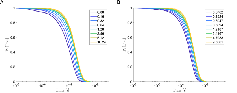
Let denote the time for the two molecules to react when each starts uniformly distributed in . The corresponding survival time distribution, , is given by
where satisfies (III.3a) with . We estimate the survival time distribution from the numerically sampled reaction times using the ecdf command in MATLAB. In Fig. 1 we demonstrates the convergence (to within sampling error) of the estimated survival time distribution of the unstructured mesh CRDDME using a Doi interaction. The survival time distributions are seen to converge as the maximum mesh width .
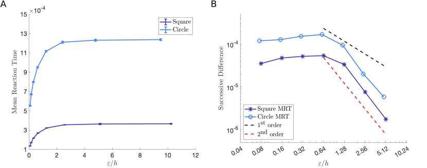
To study the rate of convergence we also examined the mean reaction time , defined by
We estimated the mean reaction time from the numerically sampled reaction times by calculating the sample mean. In Fig. 2A we show the sample mean reaction times for the Doi reaction as is varied. We see that as (i.e. ) the sample mean reaction times converge to a finite value. Figure 2B illustrates the rate of convergence using the Doi interaction by plotting the successive difference of the estimated mean reaction times as is decreased (approximately halved). For sufficiently small, the empirical rate of convergence for both reaction mechanisms is roughly second order.
IV.2 A + B C Reversible Reaction
We now consider the bimolecular reversible reaction in a system initialized with only one C molecule. The corresponding volume reactivity drift-diffusion model is given by (III.3a) and (III.3b). All molecules are assumed to have the same diffusion constant, m2s-1, and experience the same background potential defined by (IV.2). The domain is chosen to be a circle centered at with radius m. We assume a reflecting Neumann boundary condition on in each of , , and coordinates. For the forward we use the Doi reaction model
| (IV.3) |
with a reaction radius nm and . There are several different choices for , here we choose the association kernel such that it is the same as in the pure diffusive case. The corresponding dissociation rate can be obtained using (III.10)
| (IV.4) |
In the simulations, the corresponding is obtained by evaluating (IV.4) using numerical quadrature.
For all simulations the C molecule is initially placed randomly within , corresponding to the initial conditions
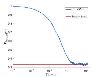
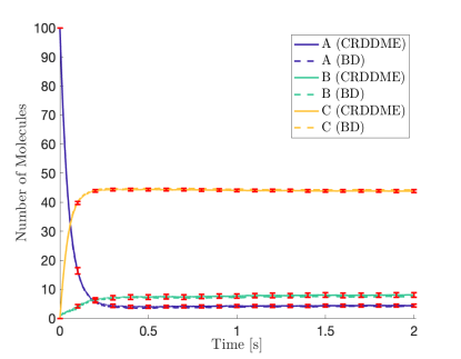
To confirm that the unstructured mesh CRDDME with reversible reaction converges to the solution of the drift-diffusion Doi VR model, we compare reaction statistics from SSA simulations against reaction statistics calculated from Brownian Dynamics (BD) simulations with a fixed time step of s. For all simulations the association rate constant in (IV.3) is set to be s-1, and the ratio of the steady-state probabilities is chosen to be . We denote by the probability the system is in the C state (i.e. the A and B molecules are bound together) at time ,
With the choice of , in the limit as
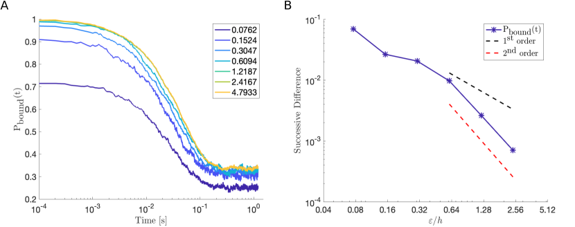
We estimated numerically by averaging the number of C molecules in the system at a fixed time over the total number of SSA (resp. BD) simulations. We demonstrate in Fig.3 that from SSA simulations agrees with from BD simulations to statistical error. Figure 4B shows the convergence of from the CRDDME simulations as the mesh width goes to zero. To demonstrate the rate of convergence, we plot the successive difference of the estimated at s as is approximately halved. In the limit that , the rate of convergence is approximately second order.
We note that with the choice of the potential function (IV.2), molecules will aggregate at the origin at steady state. As such, whenever the C molecule unbinds, the newborn A and B will quickly bind again, which gives rise to the noisiness of the steady-state .
IV.3 Multiparticle Systems
In the previous subsections, we have demonstrated the convergence of the method for basic bimolecular reactions. We now demonstrate that the method can also accurately resolve multiparticle systems by considering the following reaction system
| (IV.5) | ||||
| A |
where the first-order reaction rates s-1 and s-1, and the forward association rate is set to be s-1. The dissociation rate is determined implicitly by setting the ratio of the steady-state probabilities . The domain is chosen to be a circle of radius m centered at , discretized into elements. All molecules are assumed to diffuse at the same rate m2s-1, and the diffusive motions are affected by the same background potential defined by (IV.2). In Fig. 5 we plot the time evolution of the average number of molecules of each species from CRDDME SSA and BD simulations. The estimated average number of molecules between the CRDDME SSA and BD when averaged over simulations agree to statistical error.
IV.4 Applications
We conclude by demonstrating the ability of our method to handle realistic biochemical systems by considering a modified pattern formation model Dharan and Farago (2017); Siokis et al. (2018) upon immune synapse formation. The model involves T-cell receptors (TCRs) and pMHCs that react through the reversible bimolecular reaction
| (IV.6) |
Here we do not take into consideration LFA-1-ICAM-1 or CD28-CD80 as they interact with TCR-pMHC complexes through repulsive particle interactions Figge and Meyer-Hermann (2006); Siokis et al. (2018). The simulation domain is a circle centered at the origin with radius m (solid circle in Fig. 6), discretized into 13890 polygons. We assumed no-flux Neumann boundary conditions on the boundary of the domain. The domain is divided into two regions. The inner circular region with a radius of m is called the actin-depletion region (dotted circle in Fig. 6). The outer circular region with a radius of m (dashed circle in Fig. 6) represents the edge of the pSMAC (peripheral supra-molecular activation centers). The system is initialized with 10 free TCRs and 10 pMHCs per polygon outside the actin-depletion region, and the two species diffuse with the same diffusion constant, m2s-1. We make a simplification by assuming that free TCRs and pMHCs do not experience the actin-driven force (i.e. pure diffusion). Here we assume a pure diffusive process with the diffusion constant chosen so that it is comparable to typical values for the diffusion coefficient of T cell membrane proteins Favier et al. (2001). The binding rate is set to s-1 and the binding radius is m, which corresponds to the average length of a TCR-pMHC complex. The TCR-pMHC complex unbinds at a rate of s-1 Siokis et al. (2018); Dharan and Farago (2017).
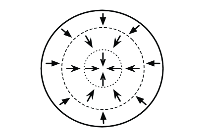
Once a free TCR binds with a free pMHC, the TCR-pMHC complex is then transported by dynein motors along microtubules and the actin retrograde flow, which together induce a centripetal force that drives the TCR-pMHC bonds to the central region of the domain. Modeling these two active processes, especially the dynein-induced forces, is highly challenging as the motor activity depends on various factors such as free ATP and the motor density. To bypass such complexity, we implement an effective active cytoskeleton force through the following potential function proposed in Dharan and Farago (2017)
| (IV.7) |
where corresponds to the magnitude of the TCR-pMHC centrally directed force Siokis et al. (2018).
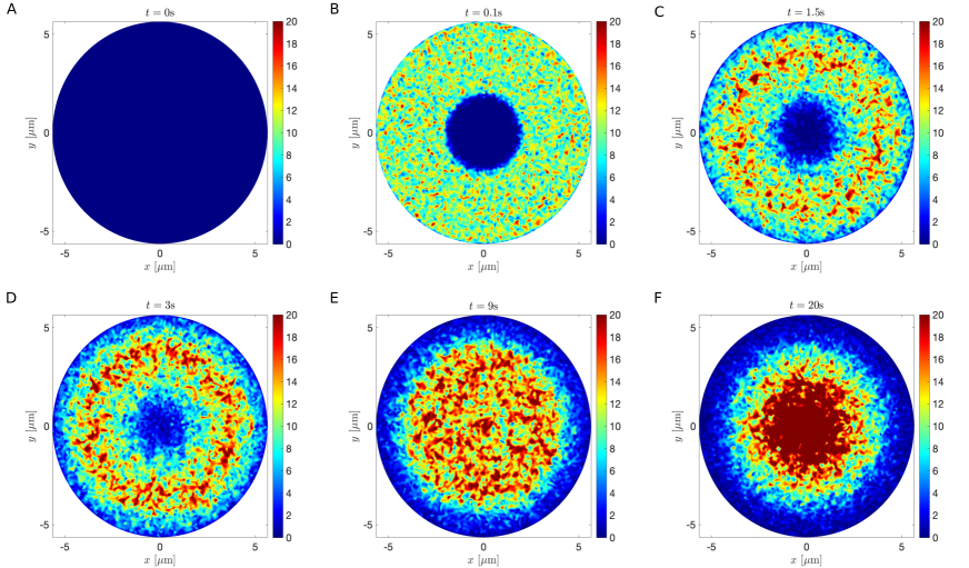
In Fig. 7 we demonstrate the TCR-pMHC complex profiles at s, s, s, s, s, and s from one CRDDME SSA simulation. Initially the TCR-pMHC complexes form a ring around the edge of the pSMAC (Fig. 7C and D) and eventually move to the actin-depletion region (Fig. 7F). We note that since LFA-1-ICAM-1 or CD28-CD80 are not considered in this simplified model, we do not observe microclusters of TCR-pMHC bonds as in Siokis et al. (2018); Dharan and Farago (2017), which highlights the importance of the repulsive particle forces between two complexes in generating microclusters that are observed upon IS formation Siokis et al. (2018).
V Discussion
By using a hybrid discretization method combining the edge-averaged finite element discretization of the drift-diffusion term and a finite volume discretization of reaction terms, we developed a convergent unstructured mesh jump process approximation, the convergent-reaction-drift-diffusion master equation (CRDDME), to the abstract volume-reactivity model with drift for reversible reactions. The CRDDME is capable of handling general bimolecular reaction kernels when the motion of molecules is influenced by background potential fields, supports unstructured polygonal meshes in two or three dimensions, and should be extendable to surfaces Ma and Isaacson (2024). As shown in Section IV the flexibility of the CRDDME approach enables the study of complex realistic biochemical systems. One benefit to the CRDDME approach is that it is consistent with key physical properties of the corresponding volume reactivity model. In particular, the reaction rates are consistent with detailed balance of reaction fluxes holding at equilibrium, and in the absence of reactions discrete versions of equilibrium Gibbs-Boltzmann distributions are recovered. Moreover, when modeling multiparticle systems, reactive transition rates are naturally given in terms of the rates derived for a minimal two-particle, , and minimal one-particle, , reaction.
Another advantage to the CRDDME approach is that it is consistent with the RDME model in its treatment of diffusive transport and linear reactions, yet converges to the underlying spatially continuous volume-reactivity model. This enables the CRDDME model to potentially reuse many RDME-based extensions for modeling spatial transport. We note that the spatial drift-diffusion transition rates we obtained could also be used without modification to define unstructured-grid RDME models that support drift due to one-body potentials.
There are still a number of directions in which the CRDDME could be improved. Here we have only discussed time-independent potential fields. An interesting future direction would be to consider time-dependent potentials. Such a generalization would enable the study of time-dependent actin flows in T cell signaling. It would also be useful to investigate other types of potentials such as particle interaction potentials that are useful to model volume exclusion in dense particle systems Siokis et al. (2018); Minton (2001); Engblom et al. (2018).
Acknowledgements.
SAI and YZ were supported by National Science Foundation DMS-1902854.References
- Su et al. (2022) Z. Su, K. Dhusia, and Y. Wu, Nat. Commun. Biol. 5, 228 (2022).
- Alberts et al. (2007) B. Alberts, A. Johnson, J. Lewis, M. Raff, K. Roberts, and P. Walter, Molecular Biology of the Cell, 5th ed. (Garland Science, New York, 2007).
- Zhang et al. (2019) Y. Zhang, L. Clemens, J. Goyette, J. Allard, O. Dushek, and S. A. Isaacson, Biophysical Journal 117, 1189 (2019).
- Larsen et al. (2020) J. B. Larsen, K. R. Rosholm, C. Kennard, S. L. Pedersen, H. K. Munch, V. Tkach, J. J. Sakon, T. Bjornholm, K. R. Weninger, P. M. Bendix, K. J. Jensen, N. S. Hatzakis, M. J. Uline, and D. Stamou, ACS central science 6, 1159 (2020).
- Rojas Molina et al. (2021) R. Rojas Molina, S. Liese, and A. Carlson, Biophysical Journal 120, 424 (2021).
- Giese et al. (2015) W. Giese, M. Eigel, S. Westerheide, C. Engwer, and E. Klipp, Phys. Biol. 12 (2015).
- Cheng et al. (2020) Y. Cheng, B. Felix, and H. Othmer, Cells. 9 (2020).
- Ma et al. (2020) J. Ma, M. Do, M. A. Le Gros, C. S. Peskin, C. A. Larabell, Y. Mori, and S. A. Isaacson, PLOS Comput Biol 16, e1008356 (19pp) (2020).
- DeMond et al. (2008) A. DeMond, K. Mossman, T. Starr, M. Dustin, and J. Groves, Biophysical Journal 94 (2008).
- Basu and Huse (2017) R. Basu and M. Huse, Trends in Cell Biology 27 (2017).
- Siokis et al. (2018) A. Siokis, P. Robert, P. Demetriou, M. Dustin, and M. Meyer-Hermann, Cell Rep. 24 (2018).
- Zhang (2015) Y. Zhang, “Particle-based stochastic reaction-diffusion methods for studying t cell signaling,” (2015).
- Isaacson (2013) S. A. Isaacson, J. Chem. Phys. 139, 054101 (2013).
- Isaacson and Zhang (2018) S. A. Isaacson and Y. Zhang, Journal of Computational Physics 374, 954 (2018).
- Teramoto and Shigesada (1967) E. Teramoto and N. Shigesada, Prog. Theor. Phys. 37, 29 (1967).
- Doi (1976a) M. Doi, J. Phys. A: Math. Gen. 9, 1465 (1976a).
- Doi (1976b) M. Doi, J. Phys. A: Math. Gen. 9, 1479 (1976b).
- Andrews and Bray (2004) S. S. Andrews and D. Bray, Physical Biology 1, 137 (2004).
- Schöneberg and Noé (2013) J. Schöneberg and F. Noé, PLOS One 8, e74261 (2013).
- Hoffmann et al. (2019) M. Hoffmann, C. Fröhner, and F. Noé, PLOS Comput. Biol. 15, e1006830 (2019).
- Fröhner and Noè (2018) C. Fröhner and F. Noè, J. of Phys. Chem. B 122, 11240 (2018).
- Tran et al. (2022) P. D. Tran, T. A. Blanpied, and P. J. Atzberger, Phys Rev E 106, 044402 (2022).
- Xu and Zikatanov (1999) J. Xu and L. Zikatanov, Mathematics of Computation 68, 1429 (1999).
- Engblom et al. (2009) S. Engblom, L. Ferm, A. Hellander, and P. Lötstedt, SIAM J. Sci. Comput. 31, 1774 (2009).
- Wang et al. (2003) H. Wang, C. S. Peskin, and T. C. Elston, J. Theor. Biol. 221, 491 (2003).
- Isaacson et al. (2011) S. A. Isaacson, D. M. McQueen, and C. S. Peskin, PNAS 108, 3815 (2011).
- Latorre et al. (2011) J. C. Latorre, P. Metzner, C. Hartmann, and C. Schütte, Commun. Math. Sci. 9, 1051 (2011).
- Dharan and Farago (2017) N. Dharan and O. Farago, Soft matter 13, 6938 (2017).
- Zhang and Isaacson (2022) Y. Zhang and S. A. Isaacson, J. Chem. Phys. 156, 204105 (2022).
- Gibson and Bruck (2000) M. A. Gibson and J. Bruck, J. Phys. Chem. A 104, 1876 (2000).
- Figge and Meyer-Hermann (2006) M. T. Figge and M. Meyer-Hermann, PLOS Comput. Biol. 2, e171 (2006).
- Favier et al. (2001) B. Favier, N. J. Burroughs, L. Wedderburn, and S. Valitutti, International Immunolog 13, 1525 (2001).
- Ma and Isaacson (2024) J. Ma and S. A. Isaacson, “A surface convergent reaction-diffusion master equation,” (2024), in preparation.
- Minton (2001) A. P. Minton, J Biol Chem 276, 10577 (2001).
- Engblom et al. (2018) S. Engblom, P. Lötstedt, and L. Meinecke, Physical Review E 98 (2018).
- Bou-Rabee and Vanden-Eijnden (2010) N. Bou-Rabee and E. Vanden-Eijnden, Communications on Pure and Applied Mathematics 63, 655 (2010).
- Griffith and Peskin (2005) B. E. Griffith and C. S. Peskin, Journal of Computational Physics 208, 75 (2005).
- Carey (1997) G. F. Carey, Computational Grids: Generations, Adaptation and Solution Strategies, 1st ed. (CRC Press, Texas, 1997).
Appendix A Accuracy of the EAFE Method
In this section, we demonstrate the second order accuracy of the EAFE discretization method. For all examples in this section, we numerically solve a time-independent PDE using either the spatial operator for the density from (II.10), or the effective transition rate matrix from (II.11). We choose to be either a square domain or a circle.
As a test problem, we consider the following steady-state problem on a square and on the circle centered at with radius one with a no-flux boundary condition
| (A.1) | |||||
where the function describing the potential field is given by
| (A.2) |
For both cases, we assume a constant diffusion constant, with inside the square and inside the circle. On the square, the forcing term was taken to be
while on the circle we chose
These choices correspond to analytical solutions given by
on the square and
on the circle.
We triangulate the domain and approximate by
with , , the nodal solution values on our triangulation. Let . The EAFE discretization of (A.1) gives
| (A.3) |
with the EAFE stiffness matrix, and the corresponding lumped mass matrix we previously derived. Here is a vector of forcing terms given by
In solving the steady-state problem (A.1), this forcing vector is evaluated using numerical quadrature.
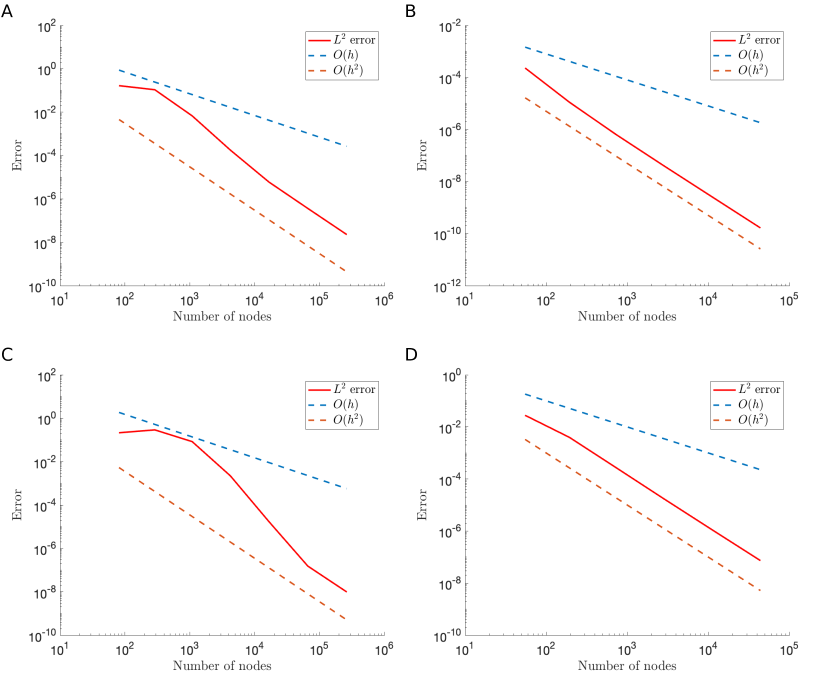
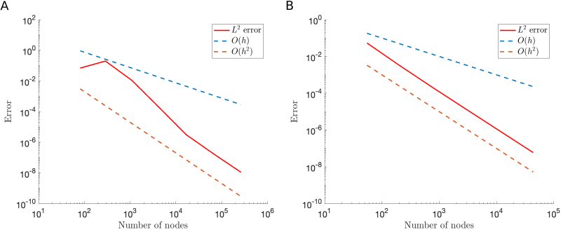
In Fig. 8A and B, we plot the error between the discerte solution and the analytical solution as the mesh size is successively halved. In both cases, we observe a second-order convergence.
To examine the convergence in a convection-dominated scenario, we increase the magnitude of the potential (A.2) by a factor of to
| (A.4) |
In Figs. 8C and D, we plot the error between the discrete solution and the PDE solution as the mesh size is successively halved. We again observe a consistent second-order convergence rate on the circle, with the convergence rate on the square becoming second order once the mesh is sufficiently small.
Finally, we repeat the same analysis on both the square and the circle using a two-well potential similar to the one in Latorre et al. (2011); Bou-Rabee and Vanden-Eijnden (2010)
| (A.5) |
For both the square and circle domains, we again observe second-order convergence as the mesh size is decreased (Fig. 9).
An empirical estimate for the rate of convergence of to in the discrete norm can be calculated using the approach of Griffith and Peskin (2005). Denote by the discrete norm of the difference in the two approximations obtained using a mesh of nodes and nodes,
| (A.6) |
where is the interpolation from the finer to the coarser meshes. We note that in our approach of mesh refinement via dividing each triangle into four congruent triangles Carey (1997), is simply the identity matrix as the finer mesh is obtained by subdividing each triangle into four congruent triangles; and therefore the the first mesh points in the finer mesh correspond to the mesh points in the coarser mesh. The empirical estimate for the rate of convergence is then defined to be
| (A.7) |
Table. 2 summarizes the empirical convergence rates in the discrete norm computed using (A.7) for the approximated solution to (A.1) on both the square domain and the circle domain. In all three cases, we observe a rate of convergence that is at least second order when solving (A.1) on a square and a circle.
| , square | , circle | , square | , circle | , square | , circle | |
| 194 | 0.92386 | 1.5813 | 2.2812 | 3.1383 | 0.4107 | 2.2258 |
| 727 | 1.8901 | 1.9203 | 0.19782 | 1.7173 | 2.0042 | 2.0509 |
| 2813 | 2.0127 | 2.0224 | 2.60487 | 1.8654 | 2.2029 | 1.9724 |
| 11065 | 2.1593 | 2.0309 | 2.90366 | 2.1669 | 2.1156 | 1.9891 |
| 43889 | 2.0848 | 2.763210 | 2.0126 | |||
Appendix B Multi-particle reaction
In this section we consider the multiparticle reaction within a bounded domain , . We will show that the discretization used in Sections II and III.3 to derive the master equation approximation for two particles (III.18) naturally leads to a master equation approximation for the multiparticle system, with transition rates for multiparticle reactions given in terms of transition rates for the two-particle case. The final rates we derive are summarized in Table 1.
We begin by formulating the multiparticle abstract volume reactivity model with reaction, using a similar notation to Isaacson (2013); Isaacson and Zhang (2018). Let denote the stochastic process for the number of A molecules in the system at time , with and defined similarly. Values of , , and are given by , , and respectively (i.e. ). Denote by the stochastic process for the position of the A molecule within the domain , with be a possible value of . The position vector of A molecules when is given by
where . In a similar way, denotes a possible value of ,
, , , , , , , , , and are defined analogously. We denote by the background one-body potential for molecules of species A when with . In what follows, we assume particles of species A experience the one-body potential, , so that when the species A state vector is it experiences the collective potential
, , , and are defined similarly.
With this notation, we let denote the probability density of having , , and with , , and . Here we assume that molecules of the same species are indistinguishable and that is symmetric respect to permutations of the molecule orderings within , , and . With this assumption, is normalized so that
Finally, we denote by the overall probability density vector at time
This density function then satisfies the forward Kolmogorov equation
| (B.1) |
Here we assume molecules cannot leave the domain , and as such a reflecting Neumann boundary condition is imposed for each component on the domain boundary . The linear operators , , correspond to drift-diffusion, the association reaction, and the dissociation reaction respectively. The drift-diffusion operator is given by
| (B.2) | ||||
where denotes the dimensional gradient operator with respect to , and and are defined similarly. Notice that this operator naturally splits into transport operators for each individual particle’s motion, so that in the absence of reactions particles would move by independent drift-diffusion processes. Moreover, this splitting means we can immediately apply our single-particle EAFE approximation to each operator independently to derive transition rates for each particle.
To define the reaction operators, and , we make use of the following notations for adding an A molecule at or removing the molecule of species A from a given state, ,
With these definitions, the reaction operator for the association reaction is given by
| (B.3) | ||||
The reaction operator for the dissociation reaction is given by
| (B.4) |
To arrive at a master equation model approximation of (B.1), we utilize the discretizations for drift-diffusion in Section II and reactions developed in Section III.3. We again consider a polygonal mesh approximation of the domain , denoted by . We let denote the multi-index label of the hyper-voxel
with , , , and defined similarly. We will use and to denote the multi-species hypervoxels. A well-mixed piecewise constant approximation of the probability the system is in the state , , with at time is given by
| (B.5a) | ||||
where denotes the vector containing the centroids of the voxels in , with and defined similarly. We denote by the overall state vector
We follow a similar approach as we employed in Isaacson and Zhang (2018). Using the EAFE discretization as in Section II to approximate each single-particle drift-diffusion operator within , integrating the action of each of the reaction operators, and , on over , and applying the locally well-mixed (i.e. piecewise constant) approximation (B.5a), the state vector satisfies the master equation
| (B.6) |
The discretized drift-diffusion operator is given by
where , , and are the single-particle species-specific EAFE discretized drift-diffusion operators, with potentials given by , , and respectively.
The association reaction operator is given by
and the backward reaction dissociation operator is given by
Denote by the stochastic process for the number of molecules of species A in voxel at time , with and defined similarly. For each species, the vector of the state at time is given by
with and defined similarly. The vector denotes the corresponding values of and is given by
The vectors and are defined similarly. Finally, we let
Following a similar analysis as in Isaacson and Zhang (2018), we can derive a master equation for
| (B.7) |
from the master equation for . Here the drift-diffusion operator is then given by
where denotes the unit vector along the th coordinate axis of .
Similarly, the association operator is given by
and the backward reaction dissociation operator is given by
We find that the effective transition rates for the mulitparticle system are then as given in Table 1, fully determined by the single-particle transport rates, the two particle association rate , and the one-particle dissociation rate .
Appendix C Pointwise detailed balance for multi-particle reaction
Denote by the equilibrium solution of (B.7). We expect it to satisfy the detailed balance condition that
| (C.1) |
As derived in Isaacson and Zhang (2018), we have that
| (C.2) |
where denotes the steady state of (B.6). Here we assume that the two representations of state are chosen to be consistent so that
with represents the cardinality of the set. and are defined similarly. Using (C.1) and (C.2), we then have the detailed balance condition for given by
| (C.3) |
which immediately implies that
| (C.4) |
This implies that
so that
| (C.5) |
Here denotes the total potential for species when the particles of species A are at the positions in . The total potentials for species and , given by and , are defined similarly. The multi-dimensional normalization factor is given by
with and defined analogously. denotes the equilibrium probability of having particles of species A, B, and C respectively. Substituting (C.5) into (C.3), we can solve for in terms of (or vice-versa)
| (C.6) |
To simplify the coefficient in the preceding relationship, we sum (C.4) over all spatial locations (i.e. over all , , and ’s) to obtain
| (C.7) | ||||
Here
and
correspond to the average association and dissociation rates with respect to the Gibbs-Boltzmann distribution for a minimal set of substrates of each reaction. We define the non-dimensional dissociation constant as their ratio,
As we expect the equilibrium probabilities, , to also satisfy detailed balance, we should have that
and hence
This is consistent with our choice that in the two-particle case studied in the main text (i.e. , , and ). (C.6) then simplifies to
Notice this is identical to (III.21). We therefore conclude that whenever the two particle association rate and the one-particle dissociation rate satisfy the detailed balance relation (III.21), the corresponding multiparticle transition rates will satisfy the (equivalent) detailed balance relation (C.6). That is, choosing and to ensure detailed balance in the two particle case is sufficient to ensure consistency of the reactive transition rates with detailed balance holding in the general multiparticle case.