RLHF from Heterogeneous Feedback via
Personalization and Preference Aggregation

Abstract

Reinforcement learning from human feedback (RLHF) has been an effective technique for aligning AI systems with human values, with remarkable successes in fine-tuning large-language models recently. Most existing RLHF paradigms make the underlying assumption that human preferences are relatively homogeneous, and can be encoded by a single reward model. In this paper, we focus on addressing the issues due to the inherent heterogeneity in human preferences, as well as their potential strategic behavior in providing feedback. Specifically, we propose two frameworks to address heterogeneous human feedback in principled ways: personalization-based one and preference-aggregation-based one. For the former, we propose two approaches based on representation learning and clustering, respectively, for learning multiple reward models that trade-off the bias (due to preference heterogeneity) and variance (due to the use of fewer data for learning each model by personalization). We then establish sample complexity guarantees for both approaches. For the latter, we aim to adhere to the single-model framework, as already deployed in the current RLHF paradigm, by carefully aggregating diverse and truthful preferences from humans. We propose two approaches based on reward and preference aggregation, respectively: the former utilizes social choice theory to aggregate individual reward models, with sample complexity guarantees; the latter directly aggregates the human feedback in the form of probabilistic opinions. Under the probabilistic-opinion-feedback model, we also develop an approach to handle strategic human labelers who may bias and manipulate the aggregated preferences with untruthful feedback. Based on the ideas in mechanism design, our approach ensures truthful preference reporting, with the induced aggregation rule maximizing social welfare functions.

1 Introduction

As AI models are becoming more powerful, there is greater emphasis on aligning their performance and priorities with the preferences of human users. In this context, reinforcement learning from human feedback (RLHF) has emerged as a promising approach, because it combines pre-trained large language models with direct human feedback (Ziegler et al., 2019; Ouyang et al., 2022; Bai et al., 2022). RLHF utilizes human feedback in the form of preferences over multiple responses in order to fine-tune the output of a pre-trained model, for example, by encouraging certain responses or types of output. The finetuning can be done by either learning a user reward model over user preference data, or by using the preference data directly (through direct preference optimization (Rafailov et al., 2024)). In either case, accurately approximating user preferences is an important task, which becomes way more challenging when the target group of users is heterogeneous (Figure 1) (Pollak and Wales, 1992; Boxall and Adamowicz, 2002).

This paper contributes to this literature by providing a holistic study of learning (different) reward models from heterogeneous user preference data. There are two major challenges in this context. The first (C1) is a pure learning one: preference data from each individual might not be sufficiently rich to construct an accurate model of heterogeneous users. The second (C2) is after learning different reward models for heterogeneous users, how to aggregate them carefully to learn a single model. Moreover, with humans (who are oftentimes viewed as rational decision-makers) involved in the loop, they might strategically misreport their preferences to manipulate this aggregated model. For example, in online rating systems, users may provide extreme feedback to disproportionately influence the overall ratings toward their viewpoint. Our approach develops ways of tackling these challenges.

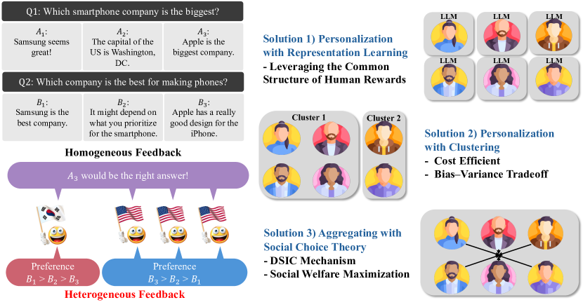
Figure 1: We demonstrate a setting where humans might have heterogeneous feedback. We provide a personalization-based framework and a human preference aggregation-based framework.

To address (C1), we adopt two approaches based on representation learning, which assume that individual reward functions share a structure through a common representation. We model each reward function as the inner product of a common representation and a parameter vector. Given the lack of sufficient individual feedback, having a shared structure by representation helps articulate each user’s reward model. The first approach constructs a personalized reward model for each user. In this approach, we find a common representation and learn each individual’s parameter vector by pooling every individual feedback. The second approach segments user preferences into clusters and learns a reward model for each cluster. This approach is useful when individual reward functions might not be available due to insufficient data. By assuming “diversity of user’s parameter vectors”, which means that individual parameter vectors span the entire space of parameters (a common assumption in multi-task learning), we show that this approach enables better sample complexity results. Leveraging data from all users helps learn the common representation, as the diversity assumption guarantees sufficient information about every dimension of the representation.

To address (C2), we first estimate the parameters for each individual’s reward model using the individual’s preference comparison data. Then, we aggregate reward models using a family of reward aggregation rules, which follows six pivotal axioms from social choice theory. We then provide sample complexities of the policy induced from the single aggregated reward model. We additionally provide a model with a different feedback type - probabilistic opinion. Concretely, instead of choosing a single answer from a pool of candidate answers, we allow the human labeler to choose a probability distribution over the answers, which indicates how much the labeler likes those answers. This type of feedback can arguably express the labeler’s preference more accurately. Moreover, probabilistic opinion feedback does not require the relationship between the human reward model and preference. We consider various aggregation rules to aggregate their probabilistic opinion vectors into one. We showed that our suggested probabilistic opinion aggregation rule is equivalent to reward aggregation rules following six pivotal axioms, under the Plackett-Luce model (Plackett, 1975; Luce, 2005).

To deal with the strategic misreport problem, we adopt a mechanism design approach whereby users correctly reporting their preferences is incentivized. We model each human labeler’s utility as a quasi-linear function, considering both the distance between her probabilistic opinion vector and the aggregated opinion vector, and the associated costs. Under this model, we show that our proposed aggregation rule maximizes social welfare. Lastly, we design an incentive-compatible mechanism to guarantee truthful reporting by inducing proper cost in the human feedback collection process.

1.1 Related Works

Reinforcement Learning from Human Feedback.

Empirical evidence has demonstrated the efficacy of incorporating human preferences into reinforcement learning (RL) for enhancing robotics (Abramson et al., 2022; Hwang et al., 2024) and for refining large-scale language models (Ziegler et al., 2019; Ouyang et al., 2022; Bai et al., 2022). These human inputs take various forms, such as rankings (Ziegler et al., 2019; Ouyang et al., 2022; Bai et al., 2022), demonstrations (Finn et al., 2016), and scalar ratings (Warnell et al., 2018). A few approaches have been explored empirically to personalize RLHF. For example, assigning fine-grained rewards to small text segments to enhance the training process (Wu et al., 2024), or training each human labeler’s reward model with Multi-Objective Reinforcement Learning perspective (Jang et al., 2023; Hwang et al., 2024) have been proposed. Moreover, (Li et al., 2024) suggested the training of each human labeler’s reward model directly using personalized feedback with human embedding obtained by the human model, and also an approach for the clustering with finding cluster embedding.

On the theory front, the studies of RLHF have received increasing research interest. The most related prior works are (Zhu et al., 2023; Zhan et al., 2023; Wang et al., 2024), where (Zhu et al., 2023) investigated the Bradley-Terry-Luce (BTL) model (Bradley and Terry, 1952) within the context of a linear reward framework; while (Zhan et al., 2023) generalized the results to encompass more general classes of reward functions. Both works concern the setting with offline preference data. Additionally, (Kim et al., 2024) provided a linear programming framework for offline reward learning. (Xiong et al., 2024) provided a theoretical analysis for KL-regularized RLHF. In the online setting, (Wang et al., 2024) established a correlation between online preference learning and online RL through a preference-to-reward interface.

Yet, to the best of our knowledge, there is no prior work that has analyzed RLHF with heterogeneous feedback with theoretical guarantees (except the recent independent works discussed in detail below).

Representation Learning.

Early work of (Baxter, 2000) established a generalization bound that hinges on the concept of a task generative model within the representation learning framework. More recently, (Tripuraneni et al., 2021; Du et al., 2021) demonstrated that, in the setup with linear representations and squared loss functions, task diversity can significantly enhance the efficiency of learning representations. Moreover, (Tripuraneni et al., 2020) provided a representation learning with general representation and general loss functions. Representation learning has been extended to the reinforcement learning setting as well. For low-rank Markov Decision Processes, where both the reward function and the probability kernel are represented through the inner products of state and action representations with certain parameters, (Agarwal et al., 2020; Ren et al., 2022; Uehara et al., 2021) explored the theoretical foundations for learning these representations. Also, (Ishfaq et al., 2024; Bose et al., 2024) analyzed the sample complexity of multi-task offline RL.

Reward and Preference Aggregation.

Preference aggregation is the process by which multiple humans’ preference orderings of various social alternatives are combined into a single, collective preference or choice (List, 2013). Arrow’s Impossibility Theorem demonstrates that no aggregation rule for preference orderings can simultaneously meet specific criteria essential for ensuring a fair and rational aggregation of each human user’s preferences into a collective decision (Arrow, 1951). Therefore, people considered replacing preference orderings with assigning real numbers to social alternatives (Sen, 2018; Moulin, 2004), which is sometimes called a reward (welfare) function in social choice theory. for each human user. (Skiadas, 2016; Moulin, 2004) provided reward (welfare) aggregation rules which satisfy several desirable properties. Furthermore, an alternative method to circumvent Arrow’s impossibility theorem involved aggregating preferences via probabilistic opinion (Stone, 1961; Lehrer and Wagner, 2012). In this approach, opinions are represented as probability assignments to specific events or propositions of interest.

Comparison with Recent Works.

While preparing the present work, we noticed two recent independent works that are closely related. Firstly, (Chakraborty et al., 2024) considered the aggregation of reward models with heterogeneous preference data, focusing on aligning with the Egalitarian principle in social choice theory. In contrast, we provide a framework with various aggregation rules and also prove that the aggregation rules we considered are also welfare-maximizing. More importantly, we design mechanisms for human feedback providers so that they can truthfully report their preferences even when they may be strategic. Moreover, we also develop another framework to handle heterogeneous preferences: the personalization-based one. Finally, we establish near-optimal sample complexity analyses for the frameworks we developed.

More recently, (Zhong et al., 2024), which is a concurrent work with this paper, provided a theoretical analysis of reward aggregation in RLHF, focusing primarily on linear representations. Our work, in comparison, considers general representation functions and general relationships between reward function and preference. Unlike (Zhong et al., 2024), where they focused on reward aggregation, we focus on personalization for every human labeler and also employ clustering techniques for personalization. (Zhong et al., 2024) and our paper also both investigated the case that reward and preference are not related. Our paper suggested a probabilistic opinion pooling with a mechanism design to effectively elicit truthful human preferences, presuming human labelers may be strategic. In contrast, (Zhong et al., 2024) analyzed an algorithm for a von Neumann winner policy, where a von Neumann winner policy is a policy that has at least a 50% chance of being preferred compared to any other policy. Moreover, (Zhong et al., 2024) also explored the Pareto efficiency of the resulting policy.

Fundamentals of Auction Theory.

Consider the sealed-bid auction mechanism (Vickrey, 1961), where each participant $i\in[N]$ privately submits a bid $b_{i}(x)$ for every possible outcome $x\in X$, whose true value is $p_{i}(x)\in\mathbb{R}$. An auction is termed a Dominant Strategic Incentive-Compatible (DSIC) auction (Roughgarden, 2010) if revealing each participant’s true valuation is a weakly dominant strategy, i.e., an individual’s optimal strategy is to bid their true valuation of the item, $b_{i}(x)=p_{i}(x)$ for all $x\in X$, irrespective of the bids $b_{-i}(x)$ submitted by others for all $x\in X$. This mechanism is also called a truthful mechanism (Roughgarden, 2010). An auction has a social-welfare-maximizing allocation rule (Roughgarden, 2010) if the outcome $x$ is $\operatorname*{arg\,max}_{x\in X}\sum_{i\in[N]}p_{i}(x)$.

Notation.

The matrix $\mathbf{O}$ denotes an all-zero matrix, while $I$ stands for an identity matrix, of proper dimensions. We use $A\succ\mathbf{O}$ to denote that matrix $A$ is a positive definite matrix. The function $\sigma$ represents the Sigmoid function, defined by $\sigma(x)=1/(1+\exp(-x))$. The notation $[K]$ denotes the set $\{1,2,\dots,K\}$. $\Delta(\mathcal{A})$ refers to a probability vector in $\mathbb{R}^{|\mathcal{A}|}$. The term $\sigma_{k}^{2}(A)$ denotes the $k$-th largest singular value of matrix $A$. A function $f(x)$ is categorized based on the complexity notation as follows: $f(x)=O(g(x))$ if there exists $C>0$ and $x_{0}$ such that $f(x)\leq Cg(x)$ holds for all $x\geq x_{0}$, $f(x)=\Omega(g(x))$ if there exists $C>0$ and $x_{0}$ such that $f(x)\geq C\cdot g(x)$ for all $x\geq x_{0}$, $f(x)=o(g(x))$ if $\lim_{x\to\infty}\frac{f(x)}{g(x)}=0$, and $f(x)=\widetilde{O}(g(x))$ if $f(n)=O(g(x)\cdot\log^{k}(g(x)))$ for some finite $k$. The vector $e_{1}$ is defined as the standard basis vector of proper dimension with the first component being $1$. For a finite-dimensional vector $x$, the norm $\|x\|_{1}$ refers to its $\ell_{1}$-norm, while $\|x\|_{2}$ refers to the $\ell_{2}$-norm, unless otherwise specified. We also define $\|x\|_{\Sigma}=\sqrt{x^{\intercal}\Sigma x}$ for a positive definite matrix $\Sigma$. For a matrix $M$, the norm $\|M\|_{F}$ denotes the Frobenius norm of $M$. The multinomial distribution is denoted by $\text{Multinomial}(p_{1},\ldots,p_{n})$, where $p_{1},\ldots,p_{n}$ are the probabilities of outcomes for each of the $n$ categories, respectively, with $\sum_{i=1}^{n}p_{i}=1$ and $p_{i}\geq 0$ for all $i\in[n]$. Kullback-Leibler (KL) divergence between two probability distributions $P,Q\in\Delta(X)$ is defined as $\sum_{x\in\text{supp}(X)}P(x)\log\left(\frac{P(x)}{Q(x)}\right)$.

2 Preliminaries

Most existing RLHF processes (for language model fine-tuning) consist of two main stages: (1) learning a model of human rewards (oftentimes from preference data), and (2) fine-tuning with the reference policy through Reinforcement Learning algorithms, e.g., Proximal Policy Optimization (PPO) (Schulman et al., 2017). It may also be possible to avoid the explicit learning of reward functions while fine-tuning the policy directly from preference data (Rafailov et al., 2024).

Markov Decision Processes.

We define the state $s$ as an element of the set of possible prompts or questions, denoted by $\mathcal{S}$, and the set of actions $a$, contained in $\mathcal{A}$, as the potential answers or responses to these questions. Consider an RLHF setting with $N$ human labelers (or users), each of whom has their own reward function. This setting can be characterized by a Markov Decision Process (MDP) with $N$ reward functions, represented by the tuple $M=(\mathcal{S},\mathcal{A},H,(P_{h})_{h\in[H]},\bm{r}=(r_{i})_{i\in[N]})$, where $H$ denotes the length of the horizon, $P_{h}:\mathcal{S}\times\mathcal{A}\mapsto\Delta(\mathcal{S})$ is the state transition probability at step $h\in[H]$, ${\mathcal{T}}:=(\mathcal{S}\times\mathcal{A})^{H}$ denotes the set of all possible trajectories, and $r_{i}:{\mathcal{T}}\rightarrow\mathbb{R}$ is the reward function for individual $i$ and trajectory $\tau\in{\mathcal{T}}$, representing the utility of human user $i$ from a sequence of responses to a given prompt. We assume $-R_{\max}\leq r_{i}(\tau)\leq R_{\max}$ for every $\tau\in{\mathcal{T}}$ and $i\in[N]$, for some $R_{\max}>0$. This reward model also covers the case that $r_{i}(\tau)=\sum_{h\in[H]}r_{h,i}(s_{h},a_{h})$, where $r_{h,i}:{\mathcal{S}}\times\mathcal{A}\to\mathbb{R}$ denotes the state-action reward function for each step $h$ and individual $i$, and $\tau=(s_{1},a_{1},s_{2},a_{2},\dots,s_{H},a_{H})$. The MDP concludes at an absorbing termination state with zero reward after $H$ steps. A policy $\pi_{h}:(\mathcal{S}\times\mathcal{A})^{h-1}\times{\mathcal{S}}\to\Delta(\mathcal{A})$ is defined as a function mapping trajectories to distributions over actions for each step $h\in[H]$ within the horizon $H$. We define the history-dependent policy class as $\Pi$. The collection of these policies across all steps is denoted by $\pi$$=(\pi_{h})_{h=1}^{H-1}$. The expected cumulative reward of a policy $\pi$ is given by $J(\pi;r_{i}):=\mathbb{E}_{\tau,\pi}[r_{i}(\tau)]$ where the expectation in the formula is taken over the distribution of the trajectories under the policy $\pi$. Trajectory occupancy measures, denoted by $d_{\pi}:{\mathcal{T}}\to[0,1]$, are defined as $d_{\pi}(\tau):=\mathbb{P}_{\pi}(\tau)$, which denotes the probability of generating trajectory $\tau$ following policy $\pi$.

Relationship between Preference and Reward Function.

For the MDP with $M=(\mathcal{S},\mathcal{A},H,(P_{h})_{h\in[H]},\bm{r}=(r_{i})_{i\in[N]})$, if we compare two trajectories $\tau_{0}$ and $\tau_{1}$, we define some random variable $o$ such that $o=0$ if $\tau_{0}\succ\tau_{1}$, and $o=1$ if $\tau_{0}\prec\tau_{1}$. Here, $\tau_{0}\succ\tau_{1}$ indicates that $\tau_{0}$ is preferred than $\tau_{1}$. We assume that $P_{r_{i}}(o=0\mid\tau_{0},\tau_{1})=\Phi(r_{i}(\tau_{0})-r_{i}(\tau_{1}))$ for all $i\in[N]$, where $\Phi:\mathbb{R}\to[0,1]$ is a monotonically increasing function, which satisfy $\Phi(x)+\Phi(-x)=1$ and $\log\Phi(x)$ is a strongly convex function. For example, $\Phi(x)=\sigma(x)$ indicates the BTL model (Definition 4.1 below), a frequently used model for the relationship between preference and reward. Also, we define $P_{\bm{r}}(\cdot\mid\tau_{0},\tau_{1}):=(P_{r_{1}}(\cdot\mid\tau_{0},\tau_{1})^{\intercal},\dots,P_{r_{N}}(\cdot\mid\tau_{0},\tau_{1})^{\intercal})^{\intercal}$. We call $P_{\bm{r}}$ and $P_{r_{i}}$ a preference probability vector induced by the reward vector $\bm{r}$ and the reward $r_{i}$.

3 Provable Personalized RLHF via Representation Learning

3.1 Learning Personalized Reward Model

In this subsection, we provide the first approach in the personalization-based framework, based on representation learning.

Reward Function Class.

We will assume that we have access to a pre-trained feature function $\phi:{\mathcal{T}}\to\mathbb{R}^{d}$, which encodes a trajectory of states and actions (i.e., questions and answers) to a $d$-dimensional feature vector. This covers the case where feature $\phi_{h}:{\mathcal{S}}\times\mathcal{A}\to\mathbb{R}^{d}$ is defined at each state-action pair, i.e., $\phi(\tau):=\sum_{h\in[H]}\phi_{h}(s_{h},a_{h})$ for trajectory $\tau=(s_{1},a_{1},\dots,s_{H},a_{H})$. For example, it is common to use the penultimate layer of an existing pre-trained LLM or other pre-trained backbones to encode a long sentence to a feature vector (Donahue et al., 2014; Gulshan et al., 2016; Tang et al., 2016).

Our first goal is to learn multiple reward models for each human user using preference datasets. First, we define the reward function class as

$$\mathcal{G}_{\bm{r}}=\left\{(\langle\psi_{\omega}(\phi(\cdot)),\theta_{i}\rangle)_{i\in[N]}{\,\big{|}\,}\psi_{\omega}\in\Psi,\theta_{i}\in\mathbb{R}^{k}\text{ and }\|\theta_{i}\|_{2}\leq B\text{ for all }i\in[N]\right\},$$

for some $B>0$, where $\Psi$ is the set of representation functions parameterized by $\omega\in\Omega$, i.e., $\Psi=\{\psi_{\omega}\mid\omega\in\Omega\}$, where $\psi_{\omega}:\mathbb{R}^{d}\to\mathbb{R}^{k}$. We assume that $d\gg k$. We denote $\boldsymbol{\theta}=(\theta_{1},\dots,\theta_{N})$, and to emphasize the relationship between reward and $(\omega,\boldsymbol{\theta})$, we will write $r_{\omega,\theta_{i}}(\cdot):=\langle\psi_{\omega}(\phi(\cdot)),\theta_{i}\rangle$ for each individual $i\in[N]$ and $\bm{r}_{\omega,\boldsymbol{\theta}}(\cdot):=(r_{\omega,\theta_{1}}(\cdot),\cdots,r_{\omega,\theta_{N}}(\cdot))^{\intercal}\in\mathbb{R}^{N}$. From this section, we will write $\bm{r}^{\star}=(r_{1}^{\star},\dots,r_{N}^{\star})$ as the underlying human reward functions.

Assumption 1 (Realizability).

We assume that the underlying true reward can be represented as $r_{i}^{\star}(\cdot)=\langle\psi^{\star}(\phi(\cdot)),\theta_{i}^{\star}\rangle$ for some representation function $\psi^{\star}\in\Psi$ (in other words, there exists some $\omega^{\star}\in\Omega$ such that $\psi_{\omega^{\star}}=\psi^{\star}$) and $\|\theta_{i}^{\star}\|_{2}\leq B$ for each individual $i\in[N]$.

To emphasize $(\omega,\boldsymbol{\theta})$, we define shorthand notation $P_{\omega,\boldsymbol{\theta}}:=P_{r_{\omega,\boldsymbol{\theta}}}$ as the preference probability induced by $r_{\omega,\boldsymbol{\theta}}$. We also write $P_{\omega,\theta}:=P_{\langle\psi_{\omega}(\phi(\cdot)),\theta\rangle}$, which is the probability induced by $\langle\psi_{\omega}(\phi(\cdot)),\theta\rangle$.

3.1.1 Algorithms

We introduce our algorithm for learning personalized policy. Compared to traditional RLHF algorithms (Ziegler et al., 2019; Ouyang et al., 2022; Zhu et al., 2023), we consider personalized reward function by representation learning.

Algorithm 1 outputs a joint estimation of $\psi^{\star}$ and $\boldsymbol{\theta}^{\star}$ with maximum likelihood estimation (MLE), together with personalized policies. The input of the algorithm is $\widehat{\mathcal{D}}=\cup_{i\in[N]}\widehat{\mathcal{D}}_{i}$ where $\widehat{\mathcal{D}}_{i}=\{(o_{i}^{(j)},\tau_{i,0}^{(j)},\tau_{i,1}^{(j)})_{j\in[N_{p}]}\}$. Here, $\tau_{i,t}^{(j)}$ is sampled from the distribution $\mu_{t}$ for $t=0,1$, and $o_{i}^{(j)}\sim P_{r^{\star}_{i}}(\cdot|\tau_{0}^{(j)},\tau_{1}^{(j)})$. First, we estimate the reward function of human users. After estimating the reward functions, we construct a confidence set for the reward function as follows: Confidence set (Equation 3.1) with $\zeta^{\prime}=C_{8}\left(k\frac{\xi^{2}\kappa^{2}\log(\mathcal{N}_{\mathcal{G}_{\bm{r}}}(1/(NN_{p}))/\delta)}{{\eta^{2}NN_{p}}}+\frac{\xi^{2}(k+\log(N/\delta))}{\eta^{2}N_{p}}+\lambda B^{2}\right)$, where $C_{8},\lambda>0$ are constants, $\xi:=\max_{x\in[-2R_{\max},2R_{\max}]}\left|\frac{\Phi^{\prime}(x)}{\Phi(x)}\right|$, $\kappa:=(\min_{x\in[-2R_{\text{max}},2R_{\text{max}}]}\Phi^{\prime}(x))^{-1}$, and $\eta:=\min_{x\in[-2R_{\max},2R_{\max}]}\left(\frac{\Phi^{\prime}(x)^{2}-\Phi^{\prime\prime}(x)\Phi(x)}{\Phi(x)^{2}}\right)$. In the case that $\Phi(x)=\sigma(x)$ (i.e. $\Phi$ is a Sigmoid), $\xi\leq 1$ and $\kappa=\eta=\frac{1}{2+\exp(-2R_{\max})+\exp(2R_{\max})}$. This confidence set will be related to Theorem 3.1. Lastly, we find the best policy based on the pessimistic expected value function. $\mu_{i,\text{ref}}$ in Algorithm 1 is a known reference trajectory distribution for individual $i\in[N]$, and it can be set as $\mu_{1}$.

Algorithm 1 Personalized RLHF via Representation Learning

  Input: Dataset $\widehat{\mathcal{D}}=\cup_{i\in[N]}\widehat{\mathcal{D}}_{i}$ where $\widehat{\mathcal{D}}_{i}=\{(o_{i}^{(j)},\tau_{i,0}^{(j)},\tau_{i,1}^{(j)})_{j\in[N_{p}]}\}$ is the preference dataset for the $i$th individual.

  Estimate $\omega^{\star}$ and $\boldsymbol{\theta}^{\star}$ by

$$(\widehat{\omega},\widehat{\boldsymbol{\theta}})\leftarrow\operatorname*{arg\,max}_{\omega\in\Omega,\|\theta_{i}\|_{2}\leq B\text{ for all }i\in[N]}\sum_{i\in[N]}\sum_{j\in[N_{p}]}\log P_{\omega,\theta_{i}}(o_{i}^{(j)}\mid\tau_{i,0}^{(j)},\tau_{i,1}^{(j)})$$

  Construct a confidence set of the reward function by

$$\mathcal{R}^{\prime}(\widehat{\mathcal{D}})\leftarrow\cap_{i\in[N]}\biggl{\{} \bm{r}_{\omega,\boldsymbol{\theta}}{\,\Big{|}\,}\frac{1}{N_{p}}\sum_{j\in[N_{p}]}\big{|}(r_{\widehat{\omega},\widehat{\theta}_{i}}(\tau_{i,0}^{(j)})-r_{\widehat{\omega},\widehat{\theta}_{i}}(\tau_{i,1}^{(j)}))-(r_{\omega,\theta_{i}}(\tau_{i,0}^{(j)})-r_{\omega,\theta_{i}}(\tau_{i,1}^{(j)}))\big{|}^{2}\leq\zeta^{\prime}\biggr{\}}$$ (3.1)

  Compute policy with respect to $\mathcal{R}(\widehat{\mathcal{D}})$ (or $\mathcal{R}^{\prime}(\widehat{\mathcal{D}})$) for all $i\in[N]$ by

$$\widehat{\pi}^{\prime}_{i}\leftarrow\operatorname*{arg\,max}_{\pi\in\Pi}\min_{\bm{r}\in\mathcal{R}^{\prime}(\widehat{\mathcal{D}})}\left(J(\pi;r_{i})-\mathbb{E}_{\tau\sim\mu_{i,\text{ref}}}[r_{i}(\tau)]\right)$$ (3.2)

  Output: $(\widehat{\omega},\widehat{\boldsymbol{\theta}},(\widehat{\pi}^{\prime}_{i})_{i\in[N]})$.

Algorithm 2 addresses a scenario where a new human user, who was not a labeler before, aims to learn their own reward models using representations previously learned by other human users, focusing solely on learning $\theta^{\star}_{0}$. They leverage the learned representation $\psi_{\widehat{\omega}}$ from Algorithm 1. The input of the algorithm is $\widehat{\mathcal{D}}_{0}=\{(o_{0}^{(j)},\tau_{0,0}^{(j)},\tau_{0,1}^{(j)})_{j\in[N_{p}]}\}$. Algorithm 2 provides an estimation of $\theta^{\star}_{0}$ with MLE using the frozen representation $\psi_{\widehat{\omega}}$. Similarly, after estimating the reward function, we construct confidence set for the MLE estimation with $\zeta=C_{8}\left(k\frac{\xi^{2}\kappa^{2}\log(\mathcal{N}_{\mathcal{G}_{\bm{r}}}(1/(NN_{p}))/\delta)}{{\eta^{2}NN_{p}}}+\frac{\xi^{2}(k+\log(1/\delta))}{\eta^{2}N_{p}}+\lambda B^{2}\right)$ for a constant $C_{8}>0$. Lastly, we find the best policy based on the pessimistic expected value function. $\mu_{0,\text{ref}}$ in Algorithm 2 is a known reference trajectory distribution.

Algorithm 2 Transferable RLHF for a New Human User via Representation Learning

  Input: Dataset $\widehat{\mathcal{D}}_{0}=\{(o_{0}^{(j)},\tau_{0,0}^{(j)},\tau_{0,1}^{(j)})_{j\in[N_{p}]}\}$ and $\widehat{\omega}$ from Algorithm 1.

  Estimate $\theta_{0}^{\star}$ by

$$\widehat{\theta}_{0}\leftarrow\operatorname*{arg\,max}_{\|\theta_{0}\|_{2}\leq B}\sum_{j\in[N_{p}]}\log P_{\widehat{\omega},\theta_{0}}(o_{0}^{(j)}\mid\tau_{0,0}^{(j)},\tau_{0,1}^{(j)})$$

  Construct a confidence set of the reward function by

$$\mathcal{R}(\widehat{\mathcal{D}})\leftarrow\biggl{\{} r_{\omega,\theta_{0}}{\,\big{|}\,}\frac{1}{N_{p}}\sum_{j\in[N_{p}]}\big{|}(r_{\widehat{\omega},\widehat{\theta}_{0}}(\tau_{0,0}^{(j)})-r_{\widehat{\omega},\widehat{\theta}_{0}}(\tau_{i,1}^{(j)}))-(r_{\omega,\theta_{0}}(\tau_{0,0}^{(j)})-r_{\omega,\theta_{0}}(\tau_{0,1}^{(j)}))\big{|}^{2}\leq\zeta\biggr{\}}$$

  Compute policy with respect to $\mathcal{R}(\widehat{\mathcal{D}})$ by

$$\widehat{\pi}_{0}\leftarrow\operatorname*{arg\,max}_{\pi\in\Pi}\min_{r_{0}\in\mathcal{R}(\widehat{\mathcal{D}}_{0})}\left(J(\pi;r_{0})-\mathbb{E}_{\tau\sim\mu_{0,\text{ref}}}[r_{0}(\tau)]\right)$$

  Output: $(\widehat{\pi}_{i})_{i\in[N]}$.

3.1.2 Results and Analyses

For ease of analysis, we consider the case where the sizes of preference datasets for each individual $i\in\{0\}\cup[N]$ are identical, i.e., $\widehat{\mathcal{D}}_{i}=\{(o_{i}^{(j)},\tau_{i,0}^{(j)},\tau_{i,1}^{(j)})_{j\in[N_{p}]}\}$, satisfies $|\widehat{\mathcal{D}}_{i}|=N_{p}$ for all $i\in\{0\}\cup[N]$. The result in this section can also be extended to the case with $|\widehat{\mathcal{D}}_{i}|=N_{p,i}$ for each individual $i$. We defer all the proofs of this section to Appendix F.

Definition 3.1 (Concentrability Coefficient).

The concentrability coefficient, with respect to a reward vector class $\mathcal{G}_{\bm{r}}$, human user $i$, a target policy $\pi_{\text{tar}}$ (which policy to compete with, which potentially can be the optimal policy $\pi_{i}^{\star}$ corresponding to $r^{\star}_{i}$), and a reference policy $\mu_{\text{ref}}$, is defined as follows:

$$C_{\bm{r}}\left(\mathcal{G}_{\bm{r}},\pi_{\text{tar }},\mu_{\text{ref }},i\right):=\max\left\{0,\sup_{\bm{r}\in\mathcal{G}_{\bm{r}}}\frac{\mathbb{E}_{\tau_{0}\sim\pi_{\text{tar }},\tau_{1}\sim\mu_{\text{ref }}}\left[r^{\star}_{i}\left(\tau_{0}\right)-r^{\star}_{i}\left(\tau_{1}\right)-r_{i}\left(\tau_{0}\right)+r_{i}\left(\tau_{1}\right)\right]}{\sqrt{\mathbb{E}_{\tau_{0}\sim\mu_{0},\tau_{1}\sim\mu_{1}}\left[\left|r^{\star}_{i}\left(\tau_{0}\right)-r^{\star}_{i}\left(\tau_{1}\right)-r_{i}\left(\tau_{0}\right)+r_{i}\left(\tau_{1}\right)\right|^{2}\right]}}\right\}.$$

We also define the concentrability coefficient of the reward scalar class in Appendix D, and we denote this as $C_{r}(\mathcal{G}_{r},\pi_{\text{tar}},\mu_{\text{ref}})$.

(Zhan et al., 2023) provides an interpretation of concentrability coefficient. For example, if $\mu_{\text{ref}}=\mu_{1}$, the value of $C_{\bm{r}}\left(\mathcal{G}_{\bm{r}},\pi_{\text{tar }},\mu_{1},i\right)\leq\sqrt{\max_{\tau\in{\mathcal{T}}}\frac{d_{\pi_{\text{tar}}}(\tau)}{\mu_{0}(\tau)}}$, so this reflects the concept of “single-policy concentrability” (Rashidinejad et al., 2021; Zanette et al., 2021; Ozdaglar et al., 2023), which is commonly assumed to be bounded in the offline RL literature.

We consider the case that $(\theta_{i})_{i\in[N]}$ are diverse (2), which is critical for improving the sample complexity of Algorithm 1 by outputting $(\widehat{\pi}_{i}^{\prime})_{i\in[N]}$. We will additionally assume the uniqueness of the representation up to the orthonormal linear transformation (3), and uniform concentration of covariance (4). These assumptions are commonly used in multi-task learning (Du et al., 2021; Tripuraneni et al., 2021; Lu et al., 2021)

Assumption 2 (Diversity).

The matrix $\Theta^{\star}=[\theta_{1}^{\star},\cdots,\theta_{N}^{\star}]\in\mathbb{R}^{k\times N}$ satisfies $\sigma_{k}^{2}(\Theta^{\star})\geq\Omega\left(N/k\right)$.

2 means that $\theta_{i}$ is evenly distributed in $\mathbb{R}^{d}$ space for $i\in[N]$, which indicates “diverse” human reward function.

Assumption 3 (Uniqueness of Representation (up to Orthonormal-Transformation)).

For any representation functions $\psi,\psi^{\prime}\in\Psi$ and $\epsilon>0$, if there exists $\{v_{i}\}_{i=1}^{T},\{v_{i}^{\prime}\}_{i=1}^{T}$, and a trajectory distribution $\mu$ that satisfy $\frac{1}{T}\sum_{i\in[T]}\mathbb{E}_{\tau\sim\mu}\|\psi(\phi(\tau))^{\top}v_{i}-\psi^{\prime}(\phi(\tau))^{\top}v_{i}^{\prime}\|^{2}\leq\epsilon,$ where $W=[v_{1},v_{2},\cdots,v_{T}]\in\mathbb{R}^{k\times T}$ satisfies $\sigma^{2}_{k}(W)\geq\Omega\left(T/k\right)$, and $\|v_{i}\|_{2}\leq B$ for all $i\in[T]$. Then, there exists a constant orthonormal matrix $P$ such that

$$\|\psi(\phi(\tau))-P\psi^{\prime}(\phi(\tau))\|^{2}\leq ck\epsilon/B$$

for all trajectory $\tau$ where $c>0$ is a constant.

This assumption posits that if two representation functions, $\psi$ and $\psi^{\prime}$, yield sufficiently small differences in expected squared norms of their inner products with corresponding vectors over trajectory distributions, then they are related by a constant orthonormal transformation. If $\psi_{\omega}(\phi(s,a)):=\omega\phi(s,a)$ where $\omega$ is ${k\times d}$ orthonormal matrix, we can prove that 3 holds with non-degenerate $\phi(s,a)$ distribution (Section F.3.2).

Definition 3.2.

Given distributions $\mu_{0},\mu_{1}$ and two representation functions $\psi,\psi^{\prime}\in\Psi$, define the covariance between $\psi$ and $\psi^{\prime}$ with respect to $\mu_{0},\mu_{1}$ to be

$$\Sigma_{\psi,\psi^{\prime}}(\mu_{0},\mu_{1}):=\mathbb{E}_{\tau_{0}\sim\mu_{0},\tau_{1}\sim\mu_{1}}[(\psi(\phi(\tau_{0}))-\psi(\phi(\tau_{1})))(\psi^{\prime}(\phi(\tau_{0}))-\psi^{\prime}(\phi(\tau_{1})))^{\intercal}]\in\mathbb{R}^{k\times k}.$$

Define the symmetric covariance as

$$\Lambda_{\psi,\psi^{\prime}}(\mu_{0},\mu_{1})=\begin{bmatrix}\Sigma_{\psi,\psi}(\mu_{0},\mu_{1})&\Sigma_{\psi,\psi^{\prime}}(\mu_{0},\mu_{1})\\ \Sigma_{\psi^{\prime},\psi}(\mu_{0},\mu_{1})&\Sigma_{\psi,\psi^{\prime}}(\mu_{0},\mu_{1})\end{bmatrix}.$$

We make the following assumption on the concentration property of the representation covariances.

Assumption 4.

(Uniform Concentrability). For any $\delta\in(0,1]$, there exists a number $N_{\text{unif}}(\Psi,\mu_{0},\mu_{1},\delta)$ such that for any $n\geq N_{\text{unif}}(\Psi,\mu_{0},\mu_{1},\delta)$, the empirical estimation $\widehat{\Lambda}_{\psi,\psi^{\prime}}(\mu_{0},\mu_{1})$ of $\Lambda_{\psi,\psi^{\prime}}(\mu_{0},\mu_{1})$ based on $n$ independent trajectory sample pairs from distributions $(\mu_{0},\mu_{1})$, with probability at least $1-\delta$, will satisfy the following inequality for all $\psi,\psi^{\prime}\in\Psi$:

$$1.1\Lambda_{\psi,\psi^{\prime}}(\mu_{0},\mu_{1})\succeq\widehat{\Lambda}_{\psi,\psi^{\prime}}(\mu_{0},\mu_{1})\succeq 0.9\Lambda_{\psi,\psi^{\prime}}(\mu_{0},\mu_{1}).$$

4 means that the empirical estimate $\widehat{\Lambda}_{\psi,\psi^{\prime}}(\mu_{0},\mu_{1})$ closely approximates the true $\Lambda_{\psi,\psi^{\prime}}(\mu_{0},\mu_{1})$ with high probability. Similarly, if $\psi_{\omega}(\phi(\tau)):=\omega\phi(\tau)$, $N_{\text{point}}(\Psi,\mu_{0},\mu_{1},\delta)=\widetilde{\mathcal{O}}(d)$ (Du et al., 2021, Claim A.1). If distributions $\mu_{0},\mu_{1}$ are clear from the context, we omit the notation $\mu_{0},\mu_{1}$ for $\Sigma_{\psi,\psi^{\prime}}(\mu_{0},\mu_{1})$ and $\Lambda_{\psi,\psi^{\prime}}(\mu_{0},\mu_{1})$. Moreover, we also write $\Sigma_{\psi,\psi}$ as $\Sigma_{\psi}$ for notational convenience.

With 2 and 3, $\psi^{\star}$ and $\psi_{\omega}$ are close up to an orthonormal matrix transformation, as asserted below:

Corollary 3.1.

(Closeness between $\psi^{\star}$ and $\psi_{\omega}$). Suppose Assumptions 1, 2, and 3 hold. For any $\delta\in(0,1]$, with probability at least $1-\delta$, if $\bm{r}_{\omega,\boldsymbol{\theta}}\in\mathcal{R}^{\prime}(\mathcal{D})$ as specified in Algorithm 1, then there exists an orthonormal matrix $P_{\omega}$ such that

$$\left[\|\psi^{\star}(\phi(\tau_{0}))-\psi^{\star}(\phi(\tau_{1}))-P_{\omega}(\psi_{\omega}(\phi(\tau_{0}))-\psi_{\omega}(\phi(\tau_{1})))\|^{2}\right]\leq k\frac{c_{\text{rep}}\kappa^{2}\log(\mathcal{N}_{\mathcal{G}_{\bm{r}}}(1/(NN_{p}))/\delta)}{{NN_{p}B^{2}}}$$

for all $\tau_{0},\tau_{1}$, where $c_{\text{rep}}>0$ is a constant.

We present the gap of the expected value function between the target policy $\pi_{i,\text{tar}}$ and the estimated policy $\widehat{\pi}_{i}$ for each individual $i\in[N]$. Here, $\pi_{i,\text{tar}}$, which may be the optimal policy $\pi_{i}^{\star}$ over $r_{i}^{\star}$, serves as the policy that $\widehat{\pi}_{i}$ will compare with.

Theorem 3.1.

(Expected Value Function Gap). Suppose Assumptions 1, 2, 3, and 4 hold. For any $\delta\in(0,1]$, all $i\in[N]$ and $\lambda>0$, with probability at least $1-\delta$, the output $\widehat{\pi}_{i}^{\prime}$ of Algorithm 1 satisfies

$$J(\pi_{i,\text{tar}};r^{\star}_{i})-J(\widehat{\pi}_{i}^{\prime};r^{\star}_{i})$$ (3.3)

$$\leq\sqrt{cC_{\bm{r}}(\mathcal{G}_{\bm{r}},\pi_{i,\text{tar}},\mu_{i,\text{ref}},i)^{2}\left(k\frac{\xi^{2}\kappa^{2}\log(\mathcal{N}_{\mathcal{G}_{\bm{r}}}(1/(NN_{p}))/\delta)}{{\eta^{2}NN_{p}}}+\frac{\xi^{2}(k+\log(N/\delta))}{\eta^{2}N_{p}}+\lambda B^{2}\right)}$$

where $c>0$ is a constant.

Lastly, we can also use the learned representation for a new human user as follows:

Theorem 3.2.

(Expected Value Function Gap for a New Human User). Suppose Assumptions 2, 3, and 4 hold. For any $\delta\in(0,1]$ and $\lambda>0$, with probability at least $1-\delta$, the output $\widehat{\pi}_{0}$ of Algorithm 2 satisfies

$$J(\pi_{0,\text{tar}};r^{\star}_{0})-J(\widehat{\pi}_{0};r^{\star}_{0})$$

$$\leq\sqrt{cC_{\bm{r}}(\mathcal{G}_{\bm{r}},\pi_{i,\text{tar}},\mu_{i,\text{ref}},i)^{2}\left(k\frac{\xi^{2}\kappa^{2}\log(\mathcal{N}_{\mathcal{G}_{\bm{r}}}(1/(NN_{p}))/\delta)}{{\eta^{2}NN_{p}}}+\frac{\xi^{2}(k+\log(1/\delta))}{\eta^{2}N_{p}}+\lambda B^{2}\right)}$$

where $c>0$ is a constant.

Remark 1 (Sample Complexity).

For Theorem 3.1, if we naively learn the personalization model without representation learning, $\mathcal{N}_{\mathcal{G}_{\bm{r}}}(1/(NN_{p}))$ will be very large. For example, if we use linear representation $\phi_{\omega}(x)=\omega x$ and $\omega$ is a $d\times k$ orthonormal matrix, then $\log(\mathcal{N}_{\mathcal{G}_{\bm{r}}}(1/NN_{p})/\delta)\leq\mathcal{O}\left((dk+Nk)\log\left(R_{\max}NN_{p}/\delta\right)\right)$ while naive personalization with

$$\mathcal{G}_{\bm{r}}^{\prime}=\left\{(\langle\phi(\cdot),\theta_{i}\rangle)_{i\in[N]}\rangle{\,\big{|}\,}\theta_{i}\in\mathbb{R}^{d}\text{ and }\|\theta_{i}\|_{2}\leq B\text{ for all }i\in[N]\right\}$$

provides $\mathcal{N}_{\mathcal{G}_{\bm{r}}^{\prime}}(1/(NN_{p}))\leq\mathcal{O}\left(Nd\log\left(R_{\max}NN_{p}/\delta\right)\right)$. Since $d\gg k$, the bound of Equation 3.3’s right-hand side has a significant improvement when we use representation learning. If the representation function class is an MLP class, we can use a known bracket number by (Bartlett et al., 2017).

We also point out that the existing technique from representation learning literature does not cover the case with general representation function learning with a log-likelihood loss function with $\mathcal{O}(1/N_{p})$ rate, to the best of our knowledge. The technical results are thus of independent interest.

Lastly, we examine the tightness of our analysis by the theoretical lower bound of the sub-optimality gap of personalization.

Theorem 3.3.

(Lower Bound for the Sub-Optimality Gap of Personalization). For any $k>6,N_{p}\geq Ck\Lambda^{2}$ and $\Lambda\geq 2$, there exists a representation function $\phi(\cdot)$ so that

$$\min_{i\in[N]}\inf_{\widehat{\bm{\pi}}}\sup_{Q\in{\rm CB}(\Lambda)}\left(\max_{\pi^{*}\in\Pi}J(\pi^{*};r_{\omega,\theta_{i}})-J(\widehat{\pi};r_{\omega,\theta_{i}})\right)\geq C\Lambda\cdot\sqrt{\frac{k}{N_{p}}},$$

where

$${\rm CB}(\Lambda)\coloneqq\left\{Q\coloneqq\left(\left\{\mu_{0},\mu_{1}\right\},\{\tau_{i,0}^{(j)},\tau_{i,1}^{(j)}\}_{i\in[N],j\in[N_{p}]},\omega,\boldsymbol{\theta}\right){\,\big{|}\,}C_{\bm{r}}^{\prime}(\mathcal{G}_{\bm{r}},\pi^{\star},\mu_{1},i)\leq\Lambda\text{ for all }i\in[N]\right\}$$

is the family of MDP with $N$ reward functions and $H=1$ instances, where

$$C_{\bm{r}}^{\prime}(\mathcal{G}_{\bm{r}},\pi^{\star},\mu_{1},i)\coloneqq\max\left\{0,\sup_{\bm{r}\in\mathcal{G}_{\bm{r}}}\frac{\mathbb{E}_{\tau_{0}\sim\pi^{\star},\tau_{1}\sim\mu_{1}}\left[r^{\star}_{i}\left(\tau_{0}\right)-r^{\star}_{i}\left(\tau_{1}\right)-r_{i}\left(\tau_{0}\right)+r_{i}\left(\tau_{1}\right)\right]}{\sqrt{\frac{1}{N_{p}}\sum_{j=1}^{N_{p}}\left[\left|r^{\star}_{i}\left(\tau_{i,0}^{(j)}\right)-r^{\star}_{i}\left(\tau_{i,1}^{(j)}\right)-r_{i}\left(\tau_{i,0}^{(j)}\right)+r_{i}\left(\tau_{i,1}^{(j)}\right)\right|^{2}\right]}}\right\}.$$ (3.4)

Our approach for personalized reward lower bound builds upon (Zhu et al., 2023, Theorem 3.10). Note that all results in this paper still hold for the new concentrability coefficient $C_{\bm{r}}^{\prime}$. By Theorem 3.3, for general representation function class, we establish that Algorithm 1 is near-optimal for the sub-optimality of the induced personalization policy, as $\log(\mathcal{N}_{\mathcal{G}_{\bm{r}}}(1/NN_{p}))$ can be small so that $\sqrt{k\frac{\log(\mathcal{N}_{\mathcal{G}_{\bm{r}}}(1/(NN_{p}))/\delta)}{NN_{p}}}$ can be dominated by $\sqrt{\frac{k}{N_{p}}}$. Note that if $\Psi$ is a linear representation class, our result for personalization (Theorem 3.1) still has a $\sqrt{k}$ gap compared to the lower bound (Theorem 3.3). This gap is also observed in (Tripuraneni et al., 2020). We will leave the sharpening of this $\sqrt{k}$ factor as a future work.

3.2 Personalized RLHF via Human User Clustering

We now provide the second approach in the personalization-based framework, through human user clustering. In particular, fine-tuning an LLM for each individual may be impractical. We thus propose an alternative approach that segments human users into clusters and fine-tunes an LLM for each cluster. This strategy entails deploying $K$ clustered models, which can be smaller than the number of human users $N$. A critical aspect of this methodology is the way to generate clusters. This clustering-based personalization has also been studied in the federated (supervised) learning literature (Mansour et al., 2020; Ghosh et al., 2020; Sattler et al., 2020). We introduce our algorithm next, based on the algorithmic idea in (Mansour et al., 2020).

3.2.1 Algorithms

We partition all the $N$ human users into $K$ clusters and find the best parameters for each cluster as follows:

$$\max_{(r_{(k)})_{k\in[K]}}\sum_{i\in[N]}\frac{1}{N}\max_{k\in[K]}\mathbb{E}_{\mathcal{D}_{i}}\left[\log P_{r_{(k)}}\left(o_{i}\mid\tau_{i,0},\tau_{i,1}\right)\right].$$

Since we only have access to the empirical data distribution, we instead solve the following problem:

$$\max_{(r_{(k)})_{k\in[K]}}\sum_{i\in[N]}\frac{1}{N}\max_{k\in[K]}\sum_{j\in[N_{p}]}\log P_{r_{(k)}}\left(o_{i}^{(j)}{\,\big{|}\,}\tau_{i,0}^{(j)},\tau_{i,1}^{(j)}\right).$$ (3.5)

Algorithm 3 outputs $K$ clustered policies and a map from human users to clusters. The input of the algorithm is $\widehat{\mathcal{D}}=\cup_{i\in[N]}\widehat{\mathcal{D}}_{i}$ where $\widehat{\mathcal{D}}_{i}=\{(o_{i}^{(j)},\tau_{i,0}^{(j)},\tau_{i,1}^{(j)})_{j\in[N_{p}]}\}$, which is the same as Algorithm 1. After estimating the representation parameter $\widehat{\omega}$, the algorithm will estimate the reward function parameters $(\widehat{\theta}_{(k)})_{k\in[K]}$ with Equation 3.6. Lastly, we find the best policy based on the expected value function. We defer a practical algorithm that uses DPO (Rafailov et al., 2024) (and also refer to Appendix D) and EM (Moon, 1996) algorithms to solve Equation 3.6 to Algorithm 6.

Algorithm 3 Personalized RLHF via Clustering

  Input: Dataset $\widehat{\mathcal{D}}=\cup_{i\in[N]}\widehat{\mathcal{D}}_{i}$ where $\widehat{\mathcal{D}}_{i}=\{(o_{i}^{(j)},\tau_{i,0}^{(j)},\tau_{i,1}^{(j)})_{j\in[N_{p}]}\}$ is the preference dataset for the $i$th individual, and $\widehat{\omega}$ form Algorithm 1.

  Learn $\theta_{(i)}$ and the clustering map $f:[N]\to[K]$ by

$$(\widehat{\theta}_{(k)})_{k\in[K]}\leftarrow\operatorname*{arg\,max}_{\|\theta_{(k)}\|_{2}\leq B\text{ for all }{k\in[K]}}\sum_{i\in[N]}\max_{k\in[K]}\sum_{j\in[N_{p}]}\log P_{\widehat{\omega},\theta_{(k)}}(o_{i}^{(j)}\mid\tau_{i,0}^{(j)},\tau_{i,1}^{(j)})$$ (3.6)

$$\widehat{f}(i)\leftarrow\operatorname*{arg\,max}_{k\in[K]}\sum_{j\in[N_{p}]}\log P_{\widehat{\omega},\widehat{\theta}_{(k)}}(o_{i}^{(j)}\mid\tau_{i,0}^{(j)},\tau_{i,1}^{(j)})\text{ for all }i\in[N]$$

  For each $k\in[K]$,

$$\widehat{\pi}_{(k)}\leftarrow\operatorname*{arg\,max}_{\pi\in\Pi}\left(J(\pi;r_{\widehat{\omega},\widehat{\theta}_{(k)}})-\mathbb{E}_{\tau\sim\mu_{1}}[r_{\widehat{\omega},\widehat{\theta}_{(k)}}(\tau)]\right).$$

  Output: $((\widehat{\pi}_{(k)})_{k\in[K]},(\widehat{\theta}_{(k)})_{k\in[K]},\widehat{\omega},\widehat{f})$.

3.2.2 Results and Analyses

To analyze the clustering-based personalization approach, we adapt the notion of label discrepancy in (Mohri and Muñoz Medina, 2012) to our RLHF setting, for preference data and a given reward function class. We defer all the proofs of this section to Appendix G.

Definition 3.3 (Label Discrepancy).

Label discrepancy for preference distribution $\bm{D}_{i}$ and $\bm{D}_{j}$, which are distributions of $(o,\tau_{0},\tau_{1})$, with reward function class $\mathcal{G}_{r}$ is defined as follows:

$$\texttt{disc}(\bm{D}_{i},\bm{D}_{j},\mathcal{G}_{r})=\max_{\bm{r}\in\mathcal{G}_{r}}\Big{|}\mathbb{E}_{\bm{D}_{i}}\log P_{r}(o\mid\tau_{1},\tau_{0})-\mathbb{E}_{\bm{D}_{j}}\log P_{r}(o\mid\tau_{1},\tau_{0})\Big{|}.$$

The discrepancy is defined as the supremum value of the difference between the log-likelihood of the preference data when taking expectations over two human dataset distributions. This quantity will be used in the analysis to characterize the gap between the log-likelihood of the estimated parameters and the underlying parameters. A similar concept is frequently used in domain adaptation (Mansour et al., 2009) and federated learning (Mansour et al., 2020).

Lemma 1 (Mansour et al. (2020)).

For any $\delta\in(0,1]$, with probability at least $1-\delta$, the output $((\widehat{\pi}_{(k)})_{k\in[K]},(\widehat{\theta}_{(k)})_{k\in[K]},\widehat{\omega},\widehat{f})$ of Algorithm 3 satisfies

$$\max_{\|\theta^{\prime}_{i}\|\leq B\text{ for all }i\in[N]}\sum_{i\in[N]}\sum_{j\in[N_{p,i}]}\log\left(\frac{P_{\widehat{\omega},\theta_{i}^{\prime}}(o_{i}^{(j)}\mid\tau_{i,0}^{(j)},\tau_{i,1}^{(j)})}{P_{\widehat{\omega},\widehat{\theta}_{\widehat{f}(i)}}(o_{i}^{(j)}\mid\tau_{i,0}^{(j)},\tau_{i,1}^{(j)})}\right)$$

$$\leq C_{\text{cluster}}NN_{p}\left(\sqrt{\frac{\log(2K/\delta)}{N_{p}}}+\sqrt{\frac{kK\log(N_{p}/k)}{N_{p}}}+\sum_{i\in[N]}\frac{1}{N}\texttt{disc}(\mathcal{D}_{i},\mathcal{C}_{\widehat{f}(i)},\mathcal{G}_{\psi_{\widehat{\omega}}})\right),$$

where $\mathcal{C}_{k}:=\cup_{\widehat{f}(i)=k}\mathcal{D}_{i}$, $C_{\text{cluster}}>0$ is a constant, and $\mathcal{G}_{\psi_{{\omega}}}:=\{r_{\omega,\theta}\mid\|\theta\|\leq B\}$ for all $\omega\in\Omega$.

Theorem 3.4.

(Total Expected Value Function Gap). Suppose Assumptions 1, 2, 3, and 4 hold. Also, assume that $C_{r}(\mathcal{G}_{r},\pi,\mu_{i,\text{ref}},i)\leq C_{\text{max}}^{\prime}$ for all policy $\pi$ and $i\in[N]$. For any $\delta\in(0,1]$, all $i\in[N]$ and $\lambda>0$, with probability at least $1-\delta$, the output $((\widehat{\pi}_{(k)})_{k\in[K]},\widehat{f})$ of Algorithm 3 satisfies

$$\sum_{i\in[N]}\left(J(\pi_{i,\text{tar}};r^{\star}_{i})-J(\widehat{\pi}_{\widehat{f}(i)};r^{\star}_{i})\right)$$

$$\leq cN\kappa\Biggl{(}\underbrace{\frac{\log(2K/\delta)}{N_{p}}+{\frac{kK\log(N_{p}/k)}{N_{p}}}}_{(i)}+{\frac{k\xi^{2}\kappa^{2}\log(\mathcal{N}_{\mathcal{G}_{r}}(1/(NN_{p}))/\delta)}{{NN_{p}}}}$$

$$\qquad\qquad\qquad+\underbrace{\left(\sum_{i\in[N]}\frac{1}{N}\texttt{disc}(\mathcal{D}_{i},\mathcal{C}_{\widehat{f}(i)},\mathcal{G}_{\psi^{\star}}))\right)^{2}}_{(ii)}+\left(\frac{\log(\mathcal{N}_{\mathcal{G}_{\psi^{\star}}}(1/NN_{p})/\delta)}{NN_{p}}\right)^{2}\Biggr{)}^{1/4},$$

where $c>0$ is a constant.

Note that Theorem 3.4 addresses the bias-variance tradeoff: as the number of clusters ($K$) increases, term (i) (variance) increases, while term (ii) (bias) decreases. Also, we note that due to the $\sqrt{kK/N_{p}}$ order on the right-hand side of Lemma 1, we have a slower rate in Theorem 3.4 than Theorem 3.1. This gap is mainly due to the fact that the analysis of Lemma 1 should cover uniformly for arbitrary $\widehat{f}$, and also due to a difference between $\max$ and expectation of $\max$, which is bounded using McDiarmid’s inequality.

Remark 2.

In contrast to the results in Section 3.1, we additionally assume $C_{r}(\mathcal{G}_{r},\pi,\mu_{1},i)\leq C_{\text{max}}^{\prime}$ in Theorem 3.4. To adopt a pessimistic approach, constructing a confidence set for clustered reward functions across all clusters is necessary. However, the ambiguity of which human user belongs to which cluster complicates this analysis, as pessimism would need to be applied to every potential cluster. Consequently, defining a confidence set for every possible clustering scenario is required, significantly complicating the analysis of the algorithm.

4 Reward and Preference Aggregation

This section adheres to the RLHF setting with a single LLM, while handling the heterogeneous human feedback by reward/preference aggregation. For reward aggregation, we first estimate individual reward functions and then aggregate these functions to form a unified reward model. In comparison, for preference aggregation, we introduce a novel framework termed “probabilistic opinion pooling”. Specifically, instead of relying on binary comparison data, human users provide feedback as probability vectors. This approach eliminates the need to aggregate heterogeneous preferences via reward functions, allowing for the direct aggregation of probabilistic opinions provided by users.

4.1 Reward Aggregation

We introduce the following reward aggregation rules (Equations (4.3) and (4.6)), which are favorable as they satisfy several pivotal axioms in social choice theory. These axioms – monotonicity, symmetry, continuity, independence of unconcerned agents, translation independence, and the Pigou-Dalton transfer principle – are crucial for ensuring fairness and consistency in the decision-making process (List, 2013; Skiadas, 2009, 2016). We present the definition of these axioms in Section H.1 for completeness. The aggregation rules are presented as follows:

$$\text{Agg}_{\alpha}(\bm{r})=\left\{\begin{array}[]{lr}\frac{1}{\alpha}\log\left(\frac{1}{N}\sum_{i\in[N]}\exp(\alpha r_{i})\right)&\alpha\neq 0\\ \frac{1}{N}\sum_{i\in[N]}r_{i}&\alpha=0\end{array}\right.$$ (4.3)

$$\text{Agg}_{\alpha}^{\prime}(\bm{r})=\left\{\begin{array}[]{lr}\frac{1}{N\alpha}\sum_{i\in[N]}(\exp(\alpha r_{i})-1)&\alpha\neq 0\\ \frac{1}{N}\sum_{i\in[N]}r_{i}&\alpha=0\end{array}\right.$$ (4.6)

where $\bm{r}=(r_{1},\dots,r_{N})^{\intercal}$ is a reward vector with trajectory input. Note that Equation 4.3 and Equation 4.6 are equivalent in the sense of the associated optimal policy, as $\log(x)$ is monotonically increasing. We can verify that $\lim_{\alpha\to-\infty}\text{Agg}_{\alpha}(\bm{r})=\min_{i\in[N]}r_{i}$ and $\lim_{\alpha\to\infty}\text{Agg}_{\alpha}(\bm{r})=\max_{i\in[N]}r_{i}$. This implies that when $\alpha$ is small (or large), the reward aggregation rule emphasizes $\min_{i\in[N]}(\text{or }\max_{i\in[N]})r_{i}$, respectively. When $\alpha=0$, Equation 4.3 represents utilitarianism, and when $\alpha\to-\infty$, Equation 4.3 represents a Leximin-based aggregation rule (List, 2013).

4.1.1 Algorithm and Analysis

Algorithm 4 outputs a joint estimation of $\psi^{\star}$ and $\boldsymbol{\theta}^{\star}$ with maximum likelihood estimation as Algorithm 1. The procedure is overall the same as Algorithm 1, except the last step for estimating the best policy for the pessimistic expected value function associated with the aggregated reward function.

Algorithm 4 RLHF with Reward Aggregation

  Input: Dataset $\widehat{\mathcal{D}}=\cup_{i\in[N]}\widehat{\mathcal{D}}_{i}$ where $\widehat{\mathcal{D}}_{i}=\{(o_{i}^{(j)},\tau_{i,0}^{(j)},\tau_{i,1}^{(j)})_{j\in[N_{p}]}\}$ is the preference dataset for the $i$th human, $\lambda>0$, and $\widehat{\omega}$ from Algorithm 1. We also use Equation 3.1 for constructing a confidence set of reward function $\mathcal{R}^{\prime}(\widehat{\mathcal{D}})$.

  Compute policy with respect to $\mathcal{R}^{\prime}(\widehat{\mathcal{D}})$ for all $i\in[N]$ by

$$\widehat{\pi}\leftarrow\operatorname*{arg\,max}_{\pi\in\Pi}\min_{\bm{r}\in\mathcal{R}^{\prime}(\widehat{\mathcal{D}})}\left(J(\pi;\text{Agg}_{\alpha}(r_{1},\dots,r_{N}))-\mathbb{E}_{\tau\sim\mu_{\text{ref}}}[\text{Agg}_{\alpha}(r_{1},\dots,r_{N})(\tau)]\right).$$ (4.7)

  Output: $(\widehat{\omega},\widehat{\boldsymbol{\theta}},\widehat{\pi})$.

Similar to the results in Theorem 3.1, we have the following theorem for Algorithm 4:

Theorem 4.1.

(Expected Value Function Gap). Suppose Assumptions 1, 2, 3, and 4 hold. For any $\delta\in(0,1]$, all $i\in[N]$ and $\lambda>0$, with probability at least $1-\delta$, the output $\widehat{\pi}$ of Algorithm 4 satisfies

$$J(\pi_{\text{tar}};\text{Agg}_{\alpha}(\bm{r}^{\star}))-J(\widehat{\pi};\text{Agg}_{\alpha}(\bm{r}^{\star}))$$

$$\leq\sqrt{c_{\alpha}C_{\bm{r}}(\mathcal{G}_{\bm{r}},\pi_{\text{tar}},\mu_{\text{ref}})^{2}\left(\frac{k\kappa^{2}\log(\mathcal{N}_{\mathcal{G}_{\bm{r}}}(1/(NN_{p}))/(\delta/N))}{{NN_{p}}}+\frac{\xi^{2}(k+\log(N/\delta))}{\eta^{2}N_{p}}+\lambda B^{2}\right)}$$

where $c_{\alpha}>0$ is a constant depending on $\alpha$, and other constants are defined in Section 3.1.1.

We defer the proof of Theorem 4.1 to Section H.2. Lastly, we prove the tightness of our analysis by providing a theoretical lower bound of the sub-optimality gap of aggregation.

Theorem 4.2.

(Lower Bound for the Sub-Optimality Gap of Aggregation). For any $k>6,N_{p}\geq Ck\Lambda^{2},\Lambda\geq 2$, and $\alpha\in\mathbb{R}$ there exists a representation function $\phi(\cdot)$ so that

$$\inf_{\widehat{\bm{\pi}}}\sup_{Q\in{\rm CB}(\Lambda)}\left(\max_{\pi^{*}\in\Pi}J(\pi^{*};\text{Agg}_{\alpha}(\bm{r}_{\omega,\boldsymbol{\theta}}))-J(\widehat{\pi};\text{Agg}_{\alpha}(\bm{r}_{\omega,\boldsymbol{\theta}}))\right)\geq C\Lambda\cdot\sqrt{\frac{k}{N_{p}}},$$

where

$${\rm CB}(\Lambda)\coloneqq\left\{Q\coloneqq\left(\left\{\mu_{0},\mu_{1}\right\},\{\tau_{i,0}^{(j)},\tau_{i,1}^{(j)}\}_{i\in[N],j\in[N_{p}]},\omega,\boldsymbol{\theta}\right){\,\big{|}\,}C_{\bm{r}}^{\prime}(\mathcal{G}_{\bm{r}},\pi^{\star},\mu_{1},i)\leq\Lambda\text{ for all }i\in[N]\right\}$$

is the family of MDP with $N$ reward functions and $H=1$ instances. $C_{\bm{r}}^{\prime}$ is defined in Equation 3.4.

By Theorem 4.2, for general representation function class, we establish that Algorithm 4 is near-optimal for the sub-optimality of the induced personalization policy.

Remark 3 (Comparison with Recent Independent Work (Zhong et al., 2024)).

(Zhong et al., 2024) also considered reward aggregation rules, adhering to the axiom of scale independence but not translation independence (Moulin, 2004). Here, scale/translation independence of the aggregation rule means that the aggregation rule should yield the same choice even if the reward functions are scaled/translated, respectively. Our theoretical results can also be extended to the reward aggregation rule in (Zhong et al., 2024). However, since we also consider the relationship of the reward aggregation rule and preference aggregation rule by probabilistic opinion pooling, which will be presented in the next section, we only present Equation 4.3 for the reward aggregation rule. (Zhong et al., 2024) also considered Nash’s bargaining (Nash, 1953), which maximizes $\prod_{i\in[N]}(r_{i}-\min r_{i})$ rather than $\prod_{i\in[N]}r_{i}$. In this case, they can also consider translation independence. Ours can also be extended by substituting $r_{i}$ to $r_{i}/\min r_{i}$ in the aggregation function (Equation 4.3), but we decided not to include it in our paper since we did not have this result in our initial draft.

4.2 Preference Aggregation with Probabilistic Opinion Data

4.2.1 RLHF with Probabilistic Opinion Feedback

Consider a set of questions $\{s^{(j)}\}_{j\in[N_{p}]}$, and for each question $s^{(j)}$, there are $K$ potential answers denoted by $\mathcal{A}^{(j)}:=\{a_{k}^{(j)}\}_{k\in[K]}$. Traditional RLHF methods involve human labelers $i\in[N]$ selecting a preferred answer from $\mathcal{A}^{(j)}$. This approach limits the human feedback to a singular choice, which, though being simple, restricts the expressiveness of human preferences.

To address this, we introduce a new setting whereby human labelers provide feedback as a probability vector $q_{i}^{(j)}\in\Delta(\mathcal{A}^{(j)})$, which is also called probabilistic opinion in social choice theory (Stone, 1961; Lehrer and Wagner, 2012). Here, $\Delta(\mathcal{A}^{(j)})$ represents the set of all possible distributions over the answers in $\mathcal{A}^{(j)}$. This allows labelers to quantify their preferences across multiple answers rather than selecting only one, and can be implemented in practice without increasing too much of overload for feedback collection.

Our setup does not assume a predefined relationship between each reward function for every human labeler and their preferences. Instead, we aggregate the diverse probabilistic preferences of multiple labelers into a consensus probability distribution over the answers. We define an aggregation function (or a probabilistic opinion pooling function), $\text{Agg-p}_{\alpha}(\bm{P})$, which takes a tuple of human preference distributions $\bm{P}=(P_{1},\dots,P_{N})\in(\Delta(\mathcal{A}))^{N}$ and maps it to a single probability distribution in $\Delta(\mathcal{A})$ where $\mathcal{A}$ is the potential answer set. For each $a\in\mathcal{A}$,

$$\text{Agg-p}_{\alpha}(\mathbf{P})(a):=\left\{\begin{array}[]{lr}\frac{\left(\sum_{i\in[N]}(P_{i}(a))^{\alpha}\right)^{1/\alpha}}{\sum_{a^{\prime}\in\mathcal{A}}\left(\sum_{i\in[N]}(P_{i}(a^{\prime}))^{\alpha}\right)^{1/\alpha}}&\alpha\neq 0\\ \frac{\left(\prod_{i\in[N]}P_{i}(a)\right)^{1/N}}{\sum_{a^{\prime}\in\mathcal{A}}\left(\prod_{i\in[N]}P_{i}(a^{\prime})\right)^{1/N}}&\alpha=0\end{array}\right..$$ (4.10)

Remark 4.

The case where $\alpha=0$ is referred to as the geometric pooling function (McConway, 1978). This function is known for preserving unanimity and not being eventwise independent, while it does satisfy external Bayesianity (Madansky, 1964; Dietrich and List, 2016). External Bayesianity mandates that updating the probabilities with new information should yield consistent results regardless of whether the update occurs before or after the aggregation process (Genest, 1984).

Interestingly, Equation 4.10, which describes the aggregation of probabilistic preferences, has a connection to Equation 4.6, concerning reward aggregation, under the assumption of the Plackett-Luce model for the relationship between reward functions and preference models (Definition 4.1). We then formalize the connection between the probabilistic opinion pooling in Equation 4.10 and the reward aggregation rule in Equation 4.3. We defer the proof of Theorem 4.3 to Section H.4.

Definition 4.1.

The Plackett-Luce (PL) model (Plackett, 1975; Luce, 2005) quantifies the likelihood that a trajectory $\tau_{k}$ is preferred over all other pairs in the set $\{\tau_{k}\}_{k\in[K]}$ by assigning it a probability defined as

$${P}_{r}\left(\tau_{k}\succ\tau_{k^{\prime}}\forall k^{\prime}\neq k{\,\big{|}\,}(\tau_{k})_{k\in[K]}\right)=\frac{\exp(r(\tau_{k}))}{\sum_{k^{\prime}\in[K]}\exp(r(\tau_{k^{\prime}}))}$$

where $r$ is the reward function for a human labeler. In the case where $k=2$, this formulation simplifies to the Bradley-Terry-Luce (BTL) Model (Bradley and Terry, 1952).

Theorem 4.3.

(Relationship between Reward Aggregation and Preference Aggregation). Suppose human preferences are modeled by the PL model, and all human labelers share a common lower bound on their reward functions. Let $(R_{i}(a))_{a\in\mathcal{A}}$ represent the reward function associated with action $a\in\mathcal{A}$ and $P_{i}\in\Delta(\mathcal{A})$ denote the corresponding probabilistic opinion for individual $i\in[N]$. Then, the preference aggregation $\text{Agg-p}_{\alpha}(\mathbf{P})$, is equivalent to the preference derived under the PL model with the aggregated rewards $(\text{Agg}_{\alpha}(\mathbf{R}(a)))_{a\in\mathcal{A}}$ for any $\alpha\in[-\infty,\infty]$.

While we generally do not presuppose any specific relationship between probabilistic opinions and reward functions, Theorem 4.3 shows that under the classical choice model of Plackett-Luce, these two aggregation rules can coincide (while the probabilistic aggregation framework may potentially handle other cases).

4.2.2 Algorithm

We provide an algorithm that uses the feedback in the form of probabilistic opinions (Algorithm 5). The only difference from the DPO algorithm (Rafailov et al., 2024) is to change the deterministic answer $a_{i}$ to the $a_{i}$ sampled based on the probabilistic opinion pooling, which is in the second line in the for loop of Algorithm 5.

Algorithm 5 Probabilistic Opinion Pooling DPO (POP-DPO)

  Input: Dataset $\widehat{\mathcal{D}}=\cup_{i\in[N]}\widehat{\mathcal{D}}_{i}$ where $\widehat{\mathcal{D}}_{i}=\{q_{i}^{(j)}(s_{i}^{(j)}),s^{(j)},i)\}_{j\in[N_{p}]}$ is the probabilistic opinion dataset for the $i$th individual, $q_{i}^{(j)}\in\Delta(\mathcal{A})$ with $|\mathcal{A}|=2$, $\beta$ is a parameter for DPO, $\alpha$ is a parameter for aggregation

  for every epoch do

     For every question $s^{(j)}$ where $j$ is in the batch, $q^{(j)}:=\text{Agg-p}_{\alpha}(\bm{q}^{(j)})$.

     Sample $a^{(j)}_{0}\sim\text{Multinomial}(q^{(j)})$ and define $a^{(j)}_{1}$ as non-selected answer.

     Run a few steps of optimization to update $\pi$ (for example, gradient ascent or Adam) to maximize

$$\sum_{j\in\text{batch}}\log\sigma\left(\beta\log\frac{\pi(a_{0}^{(j)}\mid s^{(j)})}{\pi^{\text{old}}(a_{0}^{(j)}\mid s^{(j)})}-\beta\log\frac{\pi(a_{1}^{(j)}\mid s^{(j)})}{\pi^{\text{old}}(a_{1}^{(j)}\mid s^{(j)})}\right)$$

  end for

  Output: $\pi$

5 Mechanism Design for Preference Aggregation

Suppose that human labeler $i$ ($i\in[N])$ provides preference data by probabilistic opinion $P_{i}\in\Delta(\mathcal{A})$. We now consider the natural scenario where the labelers may be strategic – given they are human beings with (certain degree of) rationality. In particular, knowing the form of preference aggregation (and the fact that they may affect the process), human labelers may provide untruthful feedback of their preference, in order to benefit more in terms of their actual utility/preference. In particular, the untruthful preference may bias the aggregated preference (that LLM will be fine-tuned over) towards their own preference, and thus manipulates the LLM output. We demonstrate the scenario more quantitatively in the following example.

An Example with Untruthful Feedback.

Consider a set of $N$ labelers evaluating two answers, where each labeler expresses a probabilistic opinion on the answers ($a_{1},a_{2}$). Specifically, suppose labeler $N$ believes that $a_{1}$ is slightly preferable to $a_{2}$, represented by the probability vector $P_{N}=(0.6,0.4)^{\intercal}$. Conversely, all other labelers $i\in[N-1]$ have probabilistic opinion favoring the second answer, represented by $P_{i}=(0.2,0.8)^{\intercal}$.

We assume that the aggregation of these opinions employs the $\text{Agg-p}_{-\infty}$ rule, defined as $\text{Agg-p}_{-\infty}(\bm{P})(a_{t})=\frac{\min_{i\in[N]}P_{i}(a_{t})}{\min_{i\in[N]}P_{i}(a_{1})+\min_{i\in[N]}P_{i}(a_{2})}$ for $t=1,2$, where $\bm{P}$ represents the matrix of probabilistic opinions across all labelers and answers. Under truthful reporting, the aggregated result would be calculated as $\text{Agg-p}_{-\infty}\left(\bm{P}\right)=\left(1/3,2/3\right)^{\intercal}$. However, labeler $N$ can strategically provide an untruthful probabilistic opinion to distort the aggregated result toward his original view: If labeler $N$ reports a distorted opinion of $P_{N}^{\prime}=(13/15,2/15)^{\intercal}$ instead of $(0.6,0.4)^{\intercal}$, the new aggregated opinion becomes $\text{Agg-p}_{-\infty}\left(\bm{P}^{\prime}\right)=\left(0.6,0.4\right)^{\intercal}$, where $\bm{P}^{\prime}=(P_{1},\dots,P_{N-1},P_{N}^{\prime})$, which aligns exactly with labeler $N$’s probabilistic opinion, while further deviating from other labelers’ actual preference. This example underscores the potential of strategic behavior in the aggregation of probabilistic opinions, and thus highlights the importance of incentivizing truthful preference reporting.

5.1 Setup

To address the untruthful feedback issue, we resort to the ideas in mechanism design (Nisan and Ronen, 1999; Börgers, 2015; Roughgarden, 2010). Specifically, we will develop mechanisms that can impose some cost on human labelers, so that they do not have the incentive to report untruthful preferences.

In this setup, we will first prove the existence of a cost function $c_{i}:\Delta(\mathcal{A})^{N}\to\mathbb{R}$ for all $i\in[N]$ that induces truthful reporting of probabilistic opinions from human labelers. Here, the input of $c_{i}$ is the probabilistic opinion of every human labeler. This is also called the dominant strategy incentive-compatible (DSIC) mechanism (Nisan and Ronen, 1999; Börgers, 2015; Roughgarden, 2010). Here incentive-compatibility means for labeler $i$, whatever the other labelers’ reports are, truthful reporting will always maximize her own utility function. Intuitively, our mechanism punishes labeler $i$ through cost $c_{i}$ for the externality she posed on other labelers, i.e., if she makes other labelers worse off based on the aggregation outcome.

Moreover, we prove that this cost function $c_{i}$ not only induce DSIC but also maximize social welfare. We denote each human labeler’s underlying (true) probabilistic opinion as $p_{i}\left(s^{\left(j\right)}\right)$ for each question $s^{(j)}$. Accounting for such cost, we define the quasi-linear utility function of individual $i$ for question $s^{(j)}$ as

$$u_{i}^{\left(j\right)}\left(p_{i}\left(s^{\left(j\right)}\right),\left(P_{i}\left(s^{\left(j\right)}\right)\right)_{i\in[N]}\right)=-d\left(p_{i}\left(s^{\left(j\right)}\right),\text{Agg-p}\left(\left(P_{i}\left(s^{\left(j\right)}\right)\right)_{i\in[N]}\right)\right)-c_{i}\left(\left(P_{i}\left(s^{\left(j\right)}\right)\right)_{i\in[N]}\right).$$

Here, $d:\Delta(\mathcal{A})\times\Delta(\mathcal{A})\to\mathbb{R}$ represents the distance between the underlying true probabilistic opinion and the aggregated preference. Moreover, we define the welfare function of individual $i$ from addressing question $s^{(j)}$ as $\text{Wel}_{i}^{(j)}(O)=-d(p_{i}(s^{(j)}),O)$ for any $O\in\Delta(\mathcal{A})$. In other words, we define utility function as subtracting cost from the welfare of individual $i$. The concepts of utility and welfare discussed in this section should not be confused with the reward used in previous sections. Here, welfare pertains to the intrinsic rewards (preferences) of individuals and the aggregation of heterogeneous human rewards (preferences).

Imposing Cost for Human Feedback Collection.

Though not being enforced in most existing RLHF frameworks, we believe it is reasonable and possible to incorporate it in the feedback collection, especially in scenarios where a single reward model (and thus a single LLM) is mandated. For example, the future large models may be regulated by some administrative agency, e.g., the government. These agencies’ objective is for social good, despite the heterogeneity in human preferences, and also possess the power to enforce cost to human labelers, e.g., via taxing. It may also be possible for big technology companies who train LLMs, e.g., OpenAI, to incentivize truthful feedback through personalized and strategic (negative) payment (which corresponds to the cost here) to human labelers.

Remark 5 (Examples of Distance Function $d$).

We can instantiate $d(p,q)$ as the KL-divergence. Also, we may instantiate $d_{\alpha}(p,q)=\text{sgn}(\alpha)\frac{1}{1-\alpha}\sum_{j\in\mathcal{A}}\left(1-p_{j}^{\alpha}q_{j}^{1-\alpha}\right)$, which is a variant of the $\alpha$-Renyi divergence for $\alpha\neq 0$. One can easily check that $d_{\alpha}(p,q)\geq 0$. In fact, one can also prove that $\lim_{\alpha\to 1}d_{\alpha}(p,q)=d(p,q)$ with $d(p,q)$ being the KL-divergence (Section H.5).

5.2 Mechanism and Guarantees

We design a mechanism inspired by the Vickery-Clarke-Groves mechanism (Vickrey, 1961; Clarke, 1971; Groves, 1973), as defined below.

Definition 5.1 (VCG Mechanism).

Assume that there are $n$ strategic agents and a finite set $X$ of outcome, and each individual $i$ has a private valuation $v_{i}$ for each outcome $x\in X$. The bidding $\bm{b}=(b_{1},\dots,b_{N})^{\intercal}\in(\mathbb{R}^{|X|})^{N}$ where $b_{i}\in\mathbb{R}^{|X|}$ is bidding for all outcome of individual $i\in[N]$. Define their utility function as $v_{i}(\bm{x}(\bm{b}))-c_{i}(\bm{b})$, where $\bm{x}:(\mathbb{R}^{|X|})^{N}\to X$ is the allocation rule and $c_{i}:(\mathbb{R}^{|X|})^{N}\to\mathbb{R}$ is the cost function. The summation of welfare function of all agents is defined as $\text{Wel}(x)=\sum_{i\in[N]}v_{i}(x)$ for all $x\in X$. The goal is to design $\bm{x}$ and $(c_{i})_{i\in[N]}$ functions to make a DSIC and welfare-maximizing mechanism. The following $\bm{x}$ and $c_{i}$ for $i\in[N]$ is DSIC welfare maximizing mechanism:

$$\bm{x}(\bm{b})=\operatorname*{arg\,max}_{x\in X}\sum_{i\in[N]}b_{i}(x),\qquad c_{i}(\bm{b})=\max_{x\in X}\sum_{j\neq i}b_{j}(x)-\sum_{j\neq i}b_{j}(\bm{x}(\bm{b}))\text{ for all }i\in[N].$$

The private valuation $v_{i}$ is corresponding to our welfare function for $i$th individual. Unfortunately, the classical VCG mechanism presents certain limitations such as it cannot be solved in polynomial time in general (Nisan and Ronen, 1999; Börgers, 2015; Roughgarden, 2010). We here adopt certain forms of allocation rule (which corresponds to the aggregation rule in our RLHF setting) and cost functions as follows, which allow the outcome set to be a simplex (with infinitely many outcomes):

$$\text{Agg-p}(\bm{P})=\operatorname*{arg\,min}_{p\in\Delta(\mathcal{A})}\sum_{i\in[N]}d(\bm{P},p),\qquad c_{i}(\bm{P})=\sum_{j\neq i}d(P_{i},\text{Agg-p}(\bm{P}))-\min_{p\in\Delta(\mathcal{A})}\sum_{j\neq i}d(P_{i},p).$$ (5.1)

Theorem 5.1.

(DSIC Welfare-Maximizing Mechanism). The aggregation rule and the cost function as in Equation 5.1 provide a DSIC welfare-maximizing mechanism.

Due to the modeling, we have an advantage compared to the original VCG mechanism. The minimization in the aggregation function can be achieved using a simple optimization method such as gradient descent, which makes our aggregation rule and cost function computation easy, which is in contrast with the original VCG mechanism.

Now, we connect our mechanism design with pre-defined preference aggregation function ($\text{Agg-p}_{\alpha}$ in Equation 4.10). Theorem 5.2 implies that Equation 4.10 is maximizing social welfare and also we are available to construct the cost function to make human feedback truthful.

Theorem 5.2.

If we set $d$ as a variant of the $\alpha$-Renyi distance for $\alpha\neq 0$ (Remark 5) and define $d$ as KL-divergence for $\alpha=0$, the DSIC welfare-maximizing aggregation rule is Equation 4.10. Therefore, aggregation rule Equation 4.10 is also welfare-maximizing with appropriate cost function.

If we assume the relationship between reward and preference follows the PL model (Definition 4.1), then Equation 4.3 implies a welfare-maximizing aggregation rule, which connects reward aggregation and mechanism design. We defer all proofs for the results in Section 5.2 to Section H.6.

Remark 6.

An analog of Theorem 5.1 and Theorem 5.2 can also be applied to reward aggregation. Additionally, under the PL model, the mechanism design for reward aggregation and preference aggregation coincide.

6 Experiments

We now conduct an empirical evaluation of our methods’ performance on a text summarization task, using the Reddit TL;DR summarization dataset and the Reddit TL;DR human feedback dataset (Stiennon et al., 2020). For the Reddit TL;DR summarization dataset, (Stiennon et al., 2020) filtered the TL;DR summarization dataset (Völske et al., 2017) to ensure quality. The Reddit TL;DR human feedback dataset is constructed with two components: comparison and axes evals. The comparison component contains labeled comparisons between pairs of summaries with workers identified by unique IDs, while the axes evals component contains ratings of summaries along three axes: accuracy, coverage, and coherence. We used GPT-J 6B (Wang and Komatsuzaki, 2021) and LLaMA3 8B models (Meta, 2024) in our experiments.

Figure 2: Accuracy of different methods with 3 times experiments. P: Personalized, C: Clustered, G(L): General (Linear) representation. Naive RLHF: original training method.

In Section 6.1, we fine-tuned the personalized reward model with Algorithm 1 and Algorithm 3, without pessimism. We ranked workers based on the number of annotated comparisons in the training split of the dataset and included the top 5 workers for training. To balance the number of samples for each worker, we took the worker with the fewest samples among the top 5 as the baseline. We then randomly sampled the same number of comparisons from the other workers so that each worker had 5,373 comparison samples, resulting in a total of 26,865 samples for training. Similarly, for the validation set, we applied the same method. We randomly sampled the same number of comparisons as the worker with the fewest samples from the top 5 workers used in training. Each worker had 1,238 samples for validation, resulting in a total of 6,190 samples for validation.

In Section 6.2, we fine-tuned the personalized reward model using Algorithm 4, without incorporating pessimism. We considered three types of reward functions: accuracy-reward, coverage-reward, and coherence-reward. Since this dataset is only publicly available for the validation set (with 8,585 samples) and the test set (with 6,313 samples), we used the validation set for fine-tuning the training set of our model and validated it with the samples in the test set. We defer other details in Appendix I.

6.1 Experiment 1: Reward Model Performance with comparison Dataset

In Experiment 1, we compared our Algorithm 1 and Algorithm 3 with naive RLHF methods. We constructed a reward model using a supervised fine-tuned language model and added a linear layer to represent individual reward functions, as in our model in Section 3.1. For the reward model structure of the general representation function, we froze the first 70% of the language model’s layers, using the outputs of these layers as the representation. For the linear representation function, we froze the entire language model and only trained the additional final layer. We used two clusters for the personalized reward model with user clustering. We evaluated the reward models based on their accuracy in correctly assigning higher rewards to chosen summaries over rejected summaries in the validation set. Our results, shown in Figure 2, indicate that clustering methods can efficiently learn the personalized reward model. Furthermore, personalization with general representation learning is necessary, as indicated by the performance gap compared to personalization with linear representation learning. Notably, for LLaMA3 8B, the performance differences between the Naive method and both PG and CG are statistically significant by t-test ($p<0.006$).

6.2 Experiment 2: Output Examples of Reward Aggregation with axes Dataset

In Experiment 2, we aggregated three axes rewards using Equation 4.3 with $\alpha=-\infty,-1,0,1,\infty$. We included representative outputs from these aggregated results in Section I.1.

Supplementary Materials for

“RLHF from Heterogeneous Feedback via

Personalization and Preference Aggregation”

Appendix A Societal Impact

Our work is mainly theoretical, and aimed at better understanding RLHF with heterogeneous feedback, with principles, algorithms, and analyses. As such, we do not anticipate any direct positive or negative societal impact from this research.

Appendix B Limitations

Our works provided overall theoretical analysis and experimental validation. However, due to the computational issue, we experimented on the 6B and 8B models, and also we did not calculate the penalty for the pessimism in our Algorithms.

Appendix C Table of Notation

Notation	Definition
N	Number of Individuals
$\mathcal{S}$	State Space
$\mathcal{A}$	Action Set
$H$	Horizon Length
$P_{h}$	Transition Probability at Horizon $h$
$\bm{r}$	Reward
$\mathcal{T}$	Trajectory Set
$\tau$	Trajectory
$J(\pi;r_{i})$	$\mathbb{E}_{\tau,\pi}\left[r_{i}(\tau)\right]$
$d_{\pi}(\tau)$	Occupancy Measure: $\mathbb{P}_{\pi}(\tau)$
$\Phi\colon\mathbb{R}\to[0,1]$	Strongly Convex Function Mapping Reward to Preference
$\sigma(x)$	Sigmoid Function: $\frac{e^{x}}{1+e^{x}}$
$P_{r_{i}}(o=0\mid\tau_{0},\tau_{1})$	$\Phi(r_{i}(\tau_{0})-r_{i}(\tau_{1}))$
$\psi_{\omega}:\mathbb{R}^{d}\to\mathbb{R}^{k}$	Representation Function
$\Psi$	$\{\psi_{\omega}\mid\omega\in\Omega\}$
$\mathcal{G}_{\bm{r}}$	Set of Reward Functions: $\{(\langle\psi_{\omega}(\phi(\cdot)),\theta_{i}\rangle)_{i\in[N]}\mid\psi_{\omega}\in\Psi,\theta_{i}\in\mathbb{R}^{k}\text{ and }\|\theta_{i}\|_{2}\leq B\text{ for all }i\in[N]\}$
$\mathcal{N}_{\mathcal{G}_{\bm{r}}}(\epsilon)$	Bracket Number of $\mathcal{G}_{\bm{r}}$ Associated with $\epsilon$
$r_{\omega,\theta_{j}}(\cdot)$	$\langle\psi_{\omega}(\phi(\cdot)),\theta_{j}\rangle$
$\bm{r}_{\omega,\boldsymbol{\theta}}(\cdot)$	$(r_{\omega,\theta_{1}}(\cdot),\cdots,r_{\omega,\theta_{N}}(\cdot))\in\mathbb{R}^{N}$
$r_{i}^{\star}(\cdot)$	Ground-truth Reward: $\langle\psi^{\star}(\phi(\cdot)),\theta_{i}^{\star}\rangle$
$\psi^{\star}(=\psi_{\omega^{\star}})$	Ground-truth Representation Function
$R_{\max}$	$-R_{\max}\leq r^{\star}_{i}(\tau)\leq R_{\max}$
$\widehat{\mathcal{D}}$	$\cup_{i\in[N]}\widehat{\mathcal{D}}_{i}$
$\widehat{\mathcal{D}}_{i}$	$\{(o_{i}^{(j)},\tau_{i,0}^{(j)},\tau_{i,1}^{(j)})_{j\in[N_{p}]}\}$
$N_{p}$	$N_{p}=|\widehat{\mathcal{D}}_{1}|=|\widehat{\mathcal{D}}_{2}|=...=|\widehat{\mathcal{D}}_{N}|$
$C_{r}\left(\mathcal{G}_{\bm{r}},\pi_{\text{tar }},\mu_{\text{ref }},i\right)$	Defined in Definition 3.1
$C_{\bm{r}}^{\prime}(\mathcal{G}_{\bm{r}},\pi^{\star},\mu_{1},i)$	Defined in Equation 3.4
$\text{Agg}_{\alpha}(\bm{r})$	Defined in Equation 4.6
$\text{Agg-p}_{\alpha}(\bm{p})(a)$	Defined in Equation 4.10

Appendix D Deferred Definition

Bracketing Number.

We modify and adopt the definition of the bracketing number of preferences introduced by (Zhan et al., 2023), with some adjustments. Consider $\mathcal{G}_{\bm{r}}$ as the class of functions representing sets of reward vectors, where each reward vector is denoted by $(r_{i})_{i\in[N]}$. Assume $g_{1}$ and $g_{2}$ maps $(\tau_{0},\tau_{1})\in{\mathcal{T}}\times{\mathcal{T}}$ to $2N$-dimensional vectors. A pair $(g_{1},g_{2})$ constitutes an $\epsilon$-bracket if for every pair of trajectories $(\tau_{0},\tau_{1})$ and for each $i\in[N]$, it holds that $g_{1}(\cdot\mid\tau_{0},\tau_{1})\leq g_{2}\left(\cdot\mid\tau_{0},\tau_{1}\right)$ and $\|g_{1}\left(\cdot\mid\tau_{0},\tau_{1}\right)-g_{2}\left(\cdot\mid\tau_{0},\tau_{1}\right)\|_{1}\leq\epsilon$. The $\epsilon$-bracketing number of $\mathcal{G}_{\bm{r}}$, denoted by $\mathcal{N}_{\mathcal{G}_{\bm{r}}}(\epsilon)$, is defined as the minimum number of $\epsilon$-brackets $\left(g_{b,1},g_{b,2}\right)_{b\in[\mathcal{N}_{\mathcal{G}_{\bm{r}}(\epsilon)}]}$ required such that for any reward vector $\bm{r}\in\mathcal{G}_{\bm{r}}$, there exists at least one bracket $b\in[\mathcal{N}_{\mathcal{G}_{\bm{r}}(\epsilon)}]$ such that for all pairs of trajectories $(\tau_{0},\tau_{1})$, $g_{b,1}(\cdot\mid\tau_{0},\tau_{1})\leq P_{\bm{r}}(\cdot\mid\tau_{0},\tau_{1})\leq g_{b,2}(\cdot\mid\tau_{0},\tau_{1})$ holds.

Concentrability Coefficient for a Reward Scalar Class

This definition is exactly the same with the concentrability coefficient of preference as outlined by (Zhan et al., 2023).

Definition D.1 (Zhan et al. (2023)).

The concentrability coefficient, with a reward vector class $\mathcal{G}_{r}$, a target policy $\pi_{\text{tar}}$ (which policy to compete with (potentially optimal policy $\pi^{\star}$)), and a reference policy $\mu_{\text{ref}}$, is defined as follows:

$$C_{r}\left(\mathcal{G}_{r},\pi_{\text{tar }},\mu_{\text{ref }}\right):=\max\left\{0,\sup_{r\in\mathcal{G}_{r}}\frac{\mathbb{E}_{\tau_{0}\sim\pi_{\text{tar }},\tau_{1}\sim\mu_{\text{ref }}}\left[r^{\star}\left(\tau_{0}\right)-r^{\star}\left(\tau_{1}\right)-r\left(\tau_{0}\right)+r\left(\tau_{1}\right)\right]}{\sqrt{\mathbb{E}_{\tau_{0}\sim\mu_{0},\tau_{1}\sim\mu_{1}}\left[\left|r^{\star}\left(\tau_{0}\right)-r^{\star}\left(\tau_{1}\right)-r\left(\tau_{0}\right)+r\left(\tau_{1}\right)\right|^{2}\right]}}\right\}.$$

Direct Preference Optimization (DPO) (Rafailov et al., 2024).

Consider the case with Markovian reward and policy, i.e., the reward $r:{\mathcal{S}}\times\mathcal{A}\to\mathbb{R}$ is a function of state $s$ and action $a$, and the policy $\pi:{\mathcal{S}}\to\Delta(\mathcal{A})$ is also depending only on the state $s$. Also, assume that we compare actions for each state rather than the whole trajectories. In the fine-tuning phase using RL, when KL-regularization with the reference policy $\pi^{\text{old}}$ is employed, the optimal policy is given by:

$$\pi(a\mid s)=\frac{1}{Z(s)}\pi^{\text{old}}(a\mid s)\exp\left(\frac{r(s,a)}{\beta}\right),$$

where $Z(s)$ serves as a normalization factor that is independent of the answer $a$, and $\beta$ represents the coefficient for KL regularization. Integrating the BTL model into this framework yields:

$$\pi^{\text{RLHF}}=\underset{\pi}{\arg\min}-\mathbb{E}_{(s,a_{0})\succ(s,a_{1})}\left[\log\sigma\left(\beta\log\frac{\pi(a_{0}\mid s)}{\pi^{\text{old}}(a_{0}\mid s)}-\beta\log\frac{\pi(a_{1}\mid s)}{\pi^{\text{old}}(a_{1}\mid s)}\right)\right],$$

where $\sigma$ denotes the Sigmoid function (Rafailov et al., 2024). This formulation bypasses the step of explicitly estimating the reward function.

Appendix E Deferred Pseudocode of Algorithms

Algorithm 6 ClusterDPO: Learning $K$ clustered policies by DPO

  Input: Dataset $\widehat{\mathcal{D}}=\cup_{i\in[N]}\widehat{\mathcal{D}}_{i}$ where $\widehat{\mathcal{D}}_{i}=\{a_{i,0}^{(j)}\succ a_{i,1}^{(j)},s_{i}^{(j)})_{j\in[N_{p}]}\}$ is the preference dataset for the $i$th individual, $\beta$ is a parameter for DPO

  Randomly select $K$ human users $p_{1},\dots,p_{K}$ and initialize $\pi_{(k)}^{0}$ for all $k\in[K]$ as

$$\pi_{(k)}^{0}\leftarrow\underset{\pi\in\Pi}{\arg\max}\sum_{j\in[N_{p}]}\log\sigma\left(\beta\log\frac{\pi(a_{p_{k},0}^{(j)}\mid s_{p_{k}}^{(j)})}{\pi^{\text{old}}(a_{p_{k},0}^{(j)}\mid s_{p_{k}}^{(j)})}-\beta\log\frac{\pi(a_{p_{k},1}^{(j)}\mid s_{p_{k}}^{(j)})}{\pi^{\text{old}}(a_{p_{k},1}^{(j)}\mid s_{p_{k}}^{(j)})}\right)$$

  Randomly initialize $f^{0}(i)$ for $i\notin\{p_{1},\dots,p_{K}\}$

  for $t\in[T]$ do

     Randomly select $K$ human users $p_{1},\dots,p_{K}$.

     for $i\in[N]$ do

        if $i\notin\{p_{1},\dots,p_{K}\}$ then

           Define $f^{t}(i)\leftarrow f^{t-1}(i)$

        end if

     end for

     Assign $f^{t}(p_{k})$ for all $k\in[K]$ as

$$f^{t}(p_{k})\leftarrow\underset{s\in[K]}{\arg\max}\sum_{j\in[N_{p}]}\log\sigma\left(\beta\log\frac{\pi_{(s)}^{t-1}(a_{p_{k},0}^{(j)}\mid s_{p_{k}}^{(j)})}{\pi^{\text{old}}(a_{p_{k},0}^{(j)}\mid s_{p_{k}}^{(j)})}-\beta\log\frac{\pi_{(s)}^{t-1}(a_{p_{k},1}^{(j)}\mid s_{p_{k}}^{(j)})}{\pi^{\text{old}}(a_{p_{k},1}^{(j)}\mid s_{p_{k}}^{(j)})}\right)$$ (E.1)

     Run a few steps of optimization to update $\pi_{(s)}^{t-1}$ for all $s\in[K]$ (for example, gradient ascent or Adam) to maximize

$$\sum_{f(p_{k})=s}\sum_{j\in[N_{p}]}\log\sigma\left(\beta\log\frac{\pi(a_{p_{k},0}^{(j)}\mid s_{p_{k}}^{(j)})}{\pi^{\text{old}}(a_{p_{k},0}^{(j)}\mid s_{p_{k}}^{(j)})}-\beta\log\frac{\pi(a_{p_{k},1}^{(j)}\mid s_{p_{k}}^{(j)})}{\pi^{\text{old}}(a_{p_{k},1}^{(j)}\mid s_{p_{k}}^{(j)})}\right)$$

and obtain $\pi_{(s)}^{t}$ for all $s\in[K]$.

  end for

  Assign $f^{T+1}(i)$ for all $i\in[N]$ as

$$f^{T+1}(i)\leftarrow\underset{s\in[K]}{\arg\max}\sum_{j\in[N_{p}]}\log\sigma\left(\beta\log\frac{\pi_{(s)}^{T}(a_{i,0}^{(j)}\mid s_{i}^{(j)})}{\pi^{\text{old}}(a_{i,0}^{(j)}\mid s_{i}^{(j)})}-\beta\log\frac{\pi_{(s)}^{T}(a_{i,1}^{(j)}\mid s_{i}^{(j)})}{\pi^{\text{old}}(a_{i,1}^{(j)}\mid s_{i}^{(j)})}\right)$$

  Output: $({\pi}_{(k)}^{T})_{k\in[K]}$ and $f^{T+1}$

Appendix F Deferred Proofs in Section 3.1

F.1 Expected Value Function Gap without Diversity Assumption

Firstly, we provide an algorithm for each reward function learning without Assumptions 2, 3, and 4.

Algorithm 7 Personalized RLHF via Representation Learning - without Diversity Assumption

  Input: Dataset $\widehat{\mathcal{D}}=\cup_{i\in[N]}\widehat{\mathcal{D}}_{i}$ where $\widehat{\mathcal{D}}_{i}=\{(o_{i}^{(j)},\tau_{i,0}^{(j)},\tau_{i,1}^{(j)})_{j\in[N_{p}]}\}$ is the preference dataset for the $i$th individual.

  Estimate $\omega^{\star}$ and $\boldsymbol{\theta}^{\star}$ by

$$(\widehat{\omega},\widehat{\boldsymbol{\theta}})\leftarrow\operatorname*{arg\,max}_{\omega\in\Omega,\|\theta_{i}\|_{2}\leq B\text{ for all }i\in[N]}\sum_{i\in[N]}\sum_{j\in[N_{p}]}\log P_{\omega,\theta_{i}}(o_{i}^{(j)}\mid\tau_{i,0}^{(j)},\tau_{i,1}^{(j)})$$

  Construct a confidence set of the reward function by

$$\mathcal{R}(\widehat{\mathcal{D}})\leftarrow\biggl{\{} \bm{r}_{\omega,\boldsymbol{\theta}}{\,\bigg{|}\,}\sum_{i\in[N]}\sum_{j\in[N_{p}]}\log P_{\omega,\theta_{i}}(o_{i}^{(j)}\mid\tau_{i,0}^{(j)},\tau_{i,1}^{(j)})\geq\sum_{i\in[N]}\sum_{j\in[N_{p}]}\log P_{\widehat{\omega},\widehat{\theta}_{i}}(o_{i}^{(j)}\mid\tau_{i,0}^{(j)},\tau_{i,1}^{(j)})-\zeta\biggr{\}}$$ (F.1)

  Compute policy with respect to $\mathcal{R}(\widehat{\mathcal{D}})$ (or $\mathcal{R}^{\prime}(\widehat{\mathcal{D}})$) for all $i\in[N]$ by

$$\widehat{\pi}_{i}\leftarrow\operatorname*{arg\,max}_{\pi\in\Pi}\min_{\bm{r}\in\mathcal{R}(\widehat{\mathcal{D}})}\left(J(\pi;r_{i})-\mathbb{E}_{\tau\sim\mu_{i,\text{ref}}}[r_{i}(\tau)]\right)$$ (F.2)

  Output: $(\widehat{\omega},\widehat{\boldsymbol{\theta}},(\widehat{\pi}_{i})_{i\in[N]})$.

• Confidence set (Equation F.1) for the MLE estimation as (Liu et al., 2022), which is also used in (Liu et al., 2023; Zhan et al., 2023; Wang et al., 2024; Zhan et al., 2022), with $\zeta=C_{1}\log(\mathcal{N}_{\mathcal{G}_{\bm{r}}}(1/(NN_{p}))/\delta)$ for a constant $C_{1}>0$, which will be related to Theorem F.1. the definition of bracketing number ($\mathcal{N}_{\mathcal{G}_{\bm{r}}}$) is deferred to Appendix D.

We will provide the expected value function gap of the output of Algorithm 7 and the reference policy.

Theorem F.1.

(Total Expected Value Function Gap). Suppose 1 holds. For any $\delta\in(0,1]$, with probability at least $1-\delta$, the output $(\widehat{\pi}_{i})_{i\in[N]}$ of Algorithm 1 satisfies

$$\sum_{i\in[N]}\left(J(\pi_{i,\text{tar}};r^{\star}_{i})-J(\widehat{\pi}_{i};r^{\star}_{i})\right)\leq\sqrt{\frac{c\kappa^{2}NC_{\max}^{2}\log(\mathcal{N}_{\mathcal{G}_{\bm{r}}}(1/NN_{p})/\delta)}{N_{p}}},$$

where $C_{\max}:=\max_{i\in[N]}C_{\bm{r}}(\mathcal{G}_{\bm{r}},\pi_{i,\text{tar}},\mu_{i,\text{ref}},i)$ and $c>0$ is a constant.

Corollary F.1.

(Expected Value Function Gap). Suppose 1 holds. For any $\delta\in(0,1]$ and all $i\in[N]$, with probability at least $1-\delta$, the output $\widehat{\pi}_{i}$ of Algorithm 1 satisfies

$$J(\pi_{i,\text{tar}};r^{\star}_{i})-J(\widehat{\pi}_{i};r^{\star}_{i})\leq\sqrt{\frac{c\kappa^{2}C_{\bm{r}}(\mathcal{G}_{\bm{r}},\pi_{i,\text{tar}},\mu_{i,\text{ref}},i)^{2}\log(\mathcal{N}_{\mathcal{G}_{\bm{r}}}(1/NN_{p})/\delta)}{N_{p}}},$$

where $c>0$ is a constant.

Note that the results above do not need any assumption on $(\theta_{i}^{\star})_{i\in[N]}$. Still, as $N_{p}\to\infty$, $\widehat{\pi}_{i}$ has comparable or better performance than the comparator policy $\pi_{i,\text{tar}}$, which approaches the optimal policy if $\pi_{i,\text{tar}}=\pi_{i}^{\star}$. We will leverage the proof of Theorem F.1 to prove Theorem 3.1. To be specific, we will improve the bound for Corollary F.1, as the gap of the expected value function does not decay with $N$, which is the number of human users. We defer the proofs of Theorem F.1 and Corollary F.1 to Section F.2.

F.2 Proof of Theorem F.1 and Corollary F.1

See F.1 See F.1 Before having a proof of Theorem F.1 and Corollary F.1, we provide two general properties of MLE estimates, which is a slightly modified version of (Zhan et al., 2023) and (Liu et al., 2022).

Lemma 2 ((Zhan et al. (2023), Lemma 1, reward vector version)).

For any $\delta\in(0,1]$, if $\bm{r}\in\mathcal{G}_{\bm{r}}$, with dataset $\widehat{\mathcal{D}}=\cup_{i\in[N]}\widehat{\mathcal{D}}_{i}$ where $\widehat{\mathcal{D}}_{i}=\{(o_{i}^{(j)},\tau_{i,0}^{(j)},\tau_{i,1}^{(j)})_{j\in[N_{p}]}\}$, $\tau_{i,0}^{(j)}\sim\mu_{0}$, $\tau_{i,1}^{(j)}\sim\mu_{1}$, and $o_{i}^{(j)}\sim P_{r^{\star}_{i}}(\cdot|\tau_{0}^{(j)},\tau_{1}^{(j)})$, there exist $C_{1}>0$ such that

$$\sum_{i\in[N]}\sum_{j\in[N_{p}]}\log\left(\frac{P_{r_{i}}(o_{i}^{(j)}\mid\tau_{i,0}^{(j)},\tau_{i,1}^{(j)})}{P_{r^{\star}_{i}}(o_{i}^{(j)}\mid\tau_{i,0}^{(j)},\tau_{i,1}^{(j)})}\right)\leq C_{1}\log(\mathcal{N}_{\mathcal{G}_{\bm{r}}}(1/(NN_{p}))/\delta)$$

holds.

Lemma 3 ((Liu et al. (2022), Proposition 14, scalar version)).

For any $\delta\in(0,1]$, with probability at least $1-\delta$, if $r\in\mathcal{G}_{r}^{\prime}$, with dataset $\widehat{\mathcal{D}}=\{(o^{(j)},\tau_{0}^{(j)},\tau_{1}^{(j)})_{j\in[M]}\}$ where $\tau_{0}^{(j)}\sim\mu_{0}$, $\tau_{1}^{(j)}\sim\mu_{1}$, and $o^{(j)}\sim P_{r^{\star}}(\cdot|\tau_{0}^{(j)},\tau_{1}^{(j)})$,

$$\mathbb{E}_{\mu_{0},\mu_{1}}\left[\|P_{r}(\cdot\mid\tau_{0}^{(j)},\tau_{1}^{(j)})-P_{r^{\star}}(\cdot\mid\tau_{0}^{(j)},\tau_{1}^{(j)})\|_{1}^{2}\right]\leq\frac{C_{2}}{M}\left(\sum_{j\in[M]}\log\left(\frac{P_{r^{\star}}(o^{(j)}\mid\tau_{0}^{(j)},\tau_{1}^{(j)})}{P_{r}(o^{(j)}\mid\tau_{0}^{(j)},\tau_{1}^{(j)})}\right)+\log(\mathcal{N}_{\mathcal{G}_{r}^{\prime}}(1/M)/\delta)\right)$$

holds where $C_{2}>0$ is a constant.

Lemma 4 ((Liu et al. (2022), Proposition 14, vector version)).

For any $\delta\in(0,1]$, with probability at least $1-\delta$, if $\bm{r}\in\mathcal{G}_{\bm{r}}^{\prime}$, with dataset $\widehat{\mathcal{D}}=\cup_{i\in[N]}\widehat{\mathcal{D}}_{i}$ where $\widehat{\mathcal{D}}_{i}=\{(o_{i}^{(j)},\tau_{i,0}^{(j)},\tau_{i,1}^{(j)})_{j\in[N_{p}]}\}$, $\tau_{i,0}^{(j)}\sim\mu_{0}$, $\tau_{i,1}^{(j)}\sim\mu_{1}$, and $o_{i}^{(j)}\sim P_{r^{\star}_{i}}(\cdot|\tau_{0}^{(j)},\tau_{1}^{(j)})$,

$$\frac{1}{N}\sum_{i\in[N]}\mathbb{E}_{\mu_{0},\mu_{1}}\left[\|P_{r_{i}}(\cdot\mid\tau_{0}^{(j)},\tau_{1}^{(j)})-P_{r^{\star}_{i}}(\cdot\mid\tau_{0}^{(j)},\tau_{1}^{(j)})\|_{1}^{2}\right]$$

$$\qquad\leq\frac{C_{2}}{NN_{p}}\left(\sum_{i\in[N]}\sum_{j\in[N_{p}]}\log\left(\frac{P_{r^{\star}_{i}}(o^{(j)}\mid\tau_{0}^{(j)},\tau_{1}^{(j)})}{P_{r_{i}}(o^{(j)}\mid\tau_{0}^{(j)},\tau_{1}^{(j)})}\right)+\log(\mathcal{N}_{\mathcal{G}_{\bm{r}}^{\prime}}(1/(NN_{p}))/\delta)\right)$$

holds where $C_{2}>0$ is a constant.

Note that $\bm{r}^{\star}$ does not need to be in $\mathcal{G}_{\bm{r}}^{\prime}$ for the above lemmas. Lemma 2 states that the log-likelihood $\log P_{\bm{r}}$ for a preference dataset generated by the reward model $\bm{r}^{\star}$ cannot exceed the log-likelihood $\log P_{\bm{r}^{\star}}$ for a preference dataset generated by the reward model $\bm{r}^{\star}$, with a gap related to the bracket number of $\mathcal{G}_{\bm{r}}$. Lemma 4 states that the $\ell_{1}$ distance between likelihood function $P_{\bm{r}^{\star}}$ and $P_{\bm{r}}$ for all $\bm{r}\in\mathcal{G}_{\bm{r}}^{\prime}$ can be bounded with the difference between log-likelihood $\log P_{\bm{r}^{\star}}$ and $\log P_{\bm{r}}$ for a preference dataset generated by the reward model $\bm{r}^{\star}$ with a gap related to the bracket number of $\mathcal{G}_{\bm{r}}^{\prime}$.

Proof of Theorem F.1 and Corollary F.1.

We define the event $\mathcal{E}_{1},\mathcal{E}_{2}$ as satisfying (Lemma 2, Lemma 4) with $\delta\leftarrow\delta/2$, respectively, so we have $\mathbb{P}(\mathcal{E}_{1}\cap\mathcal{E}_{2})>1-\delta$. We will only consider the under event $\mathcal{E}_{1}\cap\mathcal{E}_{2}$. Then, we can guarantee that

$$\sum_{i\in[N]}\sum_{j\in[N_{p}]}\log P_{\widehat{\omega},\widehat{\theta}_{i}}(o_{i}^{(j)}\mid\tau_{i,0}^{(j)},\tau_{i,1}^{(j)})$$

$$\qquad\leq\sum_{i\in[N]}\sum_{j\in[N_{p}]}\log P_{\omega^{\star},\theta^{\star}_{i}}(o_{i}^{(j)}\mid\tau_{i,0}^{(j)},\tau_{i,1}^{(j)})+C_{1}\log(\mathcal{N}_{\mathcal{G}_{\bm{r}}}(1/(NN_{p}))/\delta),$$

which indicates that $\bm{r}^{\star}(=\bm{r}_{\omega^{\star},\boldsymbol{\theta}^{\star}})\in\mathcal{R}(\widehat{\mathcal{D}})$. Moreover, by the definition of Equation F.1, if $\bm{r}_{\omega,\boldsymbol{\theta}},\bm{r}_{\omega^{\prime},\boldsymbol{\theta}^{\prime}}\in\mathcal{R}(\widehat{\mathcal{D}})$,

$$\big{|}\sum_{i\in[N]}\sum_{j\in[N_{p}]}\log P_{\omega,\theta_{i}}(o_{i}^{(j)}\mid\tau_{i,0}^{(j)},\tau_{i,1}^{(j)})-\sum_{i\in[N]}\sum_{j\in[N_{p}]}\log P_{\omega^{\prime},\theta_{i}^{\prime}}(o_{i}^{(j)}\mid\tau_{i,0}^{(j)},\tau_{i,1}^{(j)})\big{|}$$

$$\qquad\leq C_{1}\log(\mathcal{N}_{\mathcal{G}_{\bm{r}}}(1/(NN_{p}))/\delta)$$

holds, since $\sum_{i\in[N]}\sum_{j\in[N_{p}]}\log P_{\omega,\theta_{i}}(o_{i}^{(j)}\mid\tau_{i,0}^{(j)},\tau_{i,1}^{(j)})$ is bounded by $\sum_{i\in[N]}\sum_{j\in[N_{p}]}\log P_{\widehat{\omega},\widehat{\theta}_{i}}(o_{i}^{(j)}\mid\tau_{i,0}^{(j)},\tau_{i,1}^{(j)})$ by definition of $\widehat{\omega},\widehat{\boldsymbol{\theta}}$ if $r_{\omega,\boldsymbol{\theta}}\in\mathcal{G}_{\bm{r}}$. Therefore, by Lemma 4, we have

$$\frac{1}{N}\sum_{i\in[N]}\mathbb{E}_{\mu_{0},\mu_{1}}\left[\|P_{\omega,\theta_{i}}(\cdot\mid\tau_{i,0}^{(j)},\tau_{i,1}^{(j)})-P_{\omega^{\star},\theta^{\star}_{i}}(\cdot\mid\tau_{i,0}^{(j)},\tau_{i,1}^{(j)})\|_{1}^{2}\right]$$

$$\leq\frac{C_{2}}{NN_{p}}\left(\sum_{i\in[N]}\sum_{j\in[N_{p}]}\log\left(\frac{P_{\omega^{\star},\theta^{\star}_{i}}(o_{i}^{(j)}\mid\tau_{i,0}^{(j)},\tau_{i,1}^{(j)})}{P_{\omega,\theta_{i}}(o_{i}^{(j)}\mid\tau_{i,0}^{(j)},\tau_{i,1}^{(j)})}\right)+\log(\mathcal{N}_{\mathcal{G}_{\bm{r}}}(1/(NN_{p}))/\delta)\right)$$

$$\leq\frac{C_{2}}{NN_{p}}\left(C_{1}\log(\mathcal{N}_{\mathcal{G}_{\bm{r}}}(1/(NN_{p}))/\delta)+\log(\mathcal{N}_{\mathcal{G}_{\bm{r}}}(1/(NN_{p}))/\delta)\right)$$

$$=\frac{C_{3}}{NN_{p}}\log(\mathcal{N}_{\mathcal{G}_{\bm{r}}}(1/(NN_{p}))/\delta)$$

for any $\bm{r}_{\omega,\boldsymbol{\theta}}\in\mathcal{R}(\widehat{\mathcal{D}})$, where $C_{3}=C_{2}(C_{1}+1)$. Then, by the mean value theorem, for any $\bm{r}_{\omega,\boldsymbol{\theta}}\in\mathcal{R}(\widehat{\mathcal{D}})$, we have

$$\frac{1}{N}\sum_{i\in[N]}\mathbb{E}_{\mu_{0},\mu_{1}}\left[\left|(r_{\omega,\theta_{i}}(\tau_{i,0})-r_{\omega,\theta_{i}}(\tau_{i,1}))-(r_{i}^{\star}(\tau_{i,0})-r_{i}^{\star}(\tau_{i,1}))\right|^{2}\right]$$ (F.3)

$$\leq\frac{\kappa^{2}}{N}\sum_{i\in[N]}\mathbb{E}_{\mu_{0},\mu_{1}}\left[\|P_{\omega,\boldsymbol{\theta}}(\cdot\mid\tau_{i,0}^{(j)},\tau_{i,1}^{(j)},i)-P_{\omega^{\star},\boldsymbol{\theta}^{\star}}(\cdot\mid\tau_{i,0}^{(j)},\tau_{i,1}^{(j)},i)\|_{1}^{2}\right]$$

$$\leq\frac{C_{3}\kappa^{2}}{NN_{p}}\log(\mathcal{N}_{\mathcal{G}_{\bm{r}}}(1/(NN_{p}))/\delta).$$

Now, we define for all policy $\pi$,

$$r_{\pi}^{i,\text{inf}}:=\operatorname*{arg\,min}_{\bm{r}\in\mathcal{R}(\mathcal{D})}\left(J(\pi,r_{i})-\mathbb{E}_{\tau\sim\mu_{i,\text{ref}}}[r_{i}(\tau)]\right).$$

Then, we can bound the difference of the expected cumulative reward of a policy $\pi_{i,\text{tar}}$ and $\widehat{\pi}_{i}$ by

$$J(\pi_{i,\text{tar}};r^{\star}_{i})-J(\widehat{\pi}_{i};r^{\star}_{i})$$ (F.4)

$$=(J(\pi_{i,\text{tar}};r^{\star}_{i})-\mathbb{E}_{\tau\sim\mu_{i,\text{ref}}}[r^{\star}_{i}(\tau)])-(J(\widehat{\pi}_{i};r^{\star}_{i})-\mathbb{E}_{\tau\sim\mu_{i,\text{ref}}}[r^{\star}_{i}(\tau)])$$

$$\underset{(i)}{\leq}(J(\pi_{i,\text{tar}};r^{\star}_{i})-\mathbb{E}_{\tau\sim\mu_{i,\text{ref}}}[r^{\star}_{i}(\tau)])$$

$$\qquad-(J(\pi_{i,\text{tar}};r_{\pi_{i,\text{tar}}}^{i,\text{inf}})-\mathbb{E}_{\tau\sim\mu_{i,\text{ref}}}[r_{\pi_{i,\text{tar}}}^{i,\text{inf}}(\tau)])+(J(\widehat{\pi}_{j};r_{\widehat{\pi}_{i}}^{i,\text{inf}})-\mathbb{E}_{\tau\sim\mu_{i,\text{ref}}}(r_{\widehat{\pi}_{i}}^{i,\text{inf}}(\tau)))$$

$$\qquad-(J(\widehat{\pi}_{i};r^{\star}_{i})-\mathbb{E}_{\tau\sim\mu_{i,\text{ref}}}[r^{\star}_{i}(\tau)])$$

$$\underset{(ii)}{\leq}(J(\pi_{i,\text{tar}};r^{\star}_{i})-\mathbb{E}_{\tau\sim\mu_{i,\text{ref}}}[r^{\star}_{i}(\tau)])-(J(\pi_{i,\text{tar}};r_{\pi_{i,\text{tar}}}^{i,\text{inf}})-\mathbb{E}_{\tau\sim\mu_{i,\text{ref}}}[r_{\pi_{i,\text{tar}}}^{i,\text{inf}}(\tau)])$$

$$=\mathbb{E}_{\tau_{i,0}\sim\pi_{i,\text{tar}},\tau_{i,1}\sim\mu_{i,\text{ref}}}[{(r_{i}^{\star}(\tau_{i,1})-r_{i}^{\star}(\tau_{i,0}))-(r_{\pi_{i,\text{tar}}}^{i,\text{inf}}(\tau_{i,1})-r_{\pi_{i,\text{tar}}}^{i,\text{inf}}(\tau_{i,0}))}]$$

$$\leq C_{\bm{r}}(\mathcal{G}_{\bm{r}},\pi_{i,\text{tar}},\mu_{i,\text{ref}},i)\sqrt{\mathbb{E}_{\mu_{0},\mu_{1}}\left[\big{|}{(r_{i}^{\star}(\tau_{i,1})-r_{i}^{\star}(\tau_{i,0}))-(r_{\pi_{i,\text{tar}}}^{i,\text{inf}}(\tau_{i,1})-r_{\pi_{i,\text{tar}}}^{i,\text{inf}}(\tau_{i,0}))}\big{|}^{2}\right]}$$

Here, $(i)$ holds since $\widehat{\pi}_{j}$ is a distributional robust policy for $\mathcal{R}(\widehat{\mathcal{D}})$ (Equation F.1) and $(ii)$ holds due to the definition of $r_{\widehat{\pi}_{i}}^{i,\text{inf}}$. Therefore, if we sum Equation F.4 over $i\in[N]$, we have

$$\sum_{i\in[N]}\left(J(\pi_{i,\text{tar}};r^{\star}_{i})-J(\widehat{\pi}_{i};r^{\star}_{i})\right)$$

$$\leq C_{\text{max}}\sum_{i\in[N]}\sqrt{\mathbb{E}_{\mu_{0},\mu_{1}}\left[\big{|}{(r_{i}^{\star}(\tau_{i,1})-r_{i}^{\star}(\tau_{i,0}))-(r_{\pi_{i,\text{tar}}}^{i,\text{inf}}(\tau_{i,1})-r_{\pi_{i,\text{tar}}}^{i,\text{inf}}(\tau_{i,0}))}\big{|}^{2}\right]}$$

$$\leq C_{\text{max}}\sqrt{N\sum_{i\in[N]}\mathbb{E}_{\mu_{0},\mu_{1}}\left[\left|{(r_{i}^{\star}(\tau_{i,1})-r_{i}^{\star}(\tau_{i,0}))-(r_{\pi_{i,\text{tar}}}^{i,\text{inf}}(\tau_{i,1})-r_{\pi_{i,\text{tar}}}^{i,\text{inf}}(\tau_{i,0}))}\right|^{2}\right]}$$

$$\leq C_{\text{max}}\sqrt{\frac{C_{3}N\kappa^{2}\log(\mathcal{N}_{\mathcal{G}_{\bm{r}}}(1/NN_{p})/\delta)}{N_{p}}},$$

which proves Theorem F.1. Moreover, we have

$$J(\pi_{i,\text{tar}};r^{\star}_{i})-J(\widehat{\pi}_{i};r^{\star}_{i})$$

$$\leq C_{\bm{r}}(\mathcal{G}_{\bm{r}},\pi_{i,\text{tar}},\mu_{i,\text{ref}},i)\sqrt{\mathbb{E}_{\mu_{0},\mu_{1}}\left[\left|{(r_{i}^{\star}(\tau_{i,1})-r_{i}^{\star}(\tau_{i,0}))-(r_{\pi_{i,\text{tar}}}^{i,\text{inf}}(\tau_{i,1})-r_{\pi_{i,\text{tar}}}^{i,\text{inf}}(\tau_{i,0}))}\right|^{2}\right]}$$

$$\leq C_{\bm{r}}(\mathcal{G}_{\bm{r}},\pi_{i,\text{tar}},\mu_{i,\text{ref}},i)\sqrt{\sum_{i\in[N]}\mathbb{E}_{\mu_{0},\mu_{1}}\left[\left|{(r_{i}^{\star}(\tau_{i,1})-r_{i}^{\star}(\tau_{i,0}))-(r_{\pi_{i,\text{tar}}}^{i,\text{inf}}(\tau_{i,1})-r_{\pi_{i,\text{tar}}}^{i,\text{inf}}(\tau_{i,0}))}\right|^{2}\right]}$$

$$\leq C_{\bm{r}}(\mathcal{G}_{\bm{r}},\pi_{i,\text{tar}},\mu_{i,\text{ref}},i)\sqrt{\frac{C_{3}\kappa^{2}\log(\mathcal{N}_{\mathcal{G}_{\bm{r}}}(1/NN_{p})/\delta)}{N_{p}}}$$

which proves Corollary F.1. ∎

F.3 Discussion on 3

F.3.1 Comparing with (Lu et al., 2021, Assumption 6.4)

Assumption 5 ((Lu et al. (2021), Assumption 6.4)).

For any representation functions $\psi,\psi^{\prime}\in\Psi$ and $\epsilon>0$, if there exists $v,v^{\prime}\in\mathbb{R}^{d}$ that satisfy

$$\mathbb{E}\|\psi(x)^{\top}v-\psi^{\prime}(x)^{\top}v^{\prime}\|^{2}\leq\epsilon$$

Then there exists a constant invertible matrix $P$ such that

$$\|\psi(x)-P\psi^{\prime}(x)\|^{2}\leq o(\epsilon/\|v\|^{2})=o(\epsilon/\|v^{\prime}\|^{2}).$$

for all $x$.

3 bears similarity to 5; however, the latter is notably more stringent. For instance, consider the case where $v=v^{\prime}=e_{1}$ without loss of generality. If it holds that $\mathbb{E}\|\psi_{1}(x)-\psi^{\prime}_{1}(x)\|^{2}\leq\epsilon$, then it implies $\psi\sim P\psi^{\prime}$. In this context, $\psi_{1}$ and $\psi^{\prime}_{1}$ represent the first coordinates of $\psi$ and $\psi^{\prime}$, respectively. The assumption that similarity in the first coordinate necessitates equivalence of the entire representations ($\psi\sim P\psi^{\prime}$) is a strong assumption.

F.3.2 Case Study (Linear Representation): $\psi_{\omega}(x)=\omega x$ and $\omega$ is an Orthonormal Matrix

Proposition 1.

Assume that $\psi_{\omega}(\phi(\tau))=\omega\phi(\tau)$ where $\omega$ is a ${k\times d}$ orthornormal matrix. For any representation functions $\psi_{\omega},\psi_{\omega^{\prime}}\in\Psi$ and $\epsilon>0$, if there exists $\{v_{i}\}_{i=1}^{T},\{v_{i}^{\prime}\}_{i=1}^{T}$, and a trajectory distribution $\mu$ that satisfy

$$\frac{1}{T}\sum_{i\in[T]}\mathbb{E}_{\tau\sim\mu}\|\psi_{\omega}(\phi(\tau))^{\top}v_{i}-\psi_{\omega^{\prime}}(\phi(\tau))^{\top}v_{i}^{\prime}\|^{2}\leq\epsilon$$ (F.5)

dand $V=[v_{1},v_{2},\cdots,v_{T}]\in\mathbb{R}^{k\times T}$ satisfies $\sigma^{2}_{k}(W)\geq\Omega\left(T/k\right)$, and $\|v_{i}\|_{2}\leq B$ for all $i\in[T]$. If $\Sigma:=\mathbb{E}_{\mu}[\phi(\tau)\phi(\tau)^{\intercal}]\succ\mathbf{O}$, then there exists a constant invertible matrix $P$ such that

$$\|\psi_{\omega}(\phi(\tau))-P\psi_{\omega^{\prime}}(\phi(\tau))\|^{2}\leq ck\epsilon/B$$

where $c>0$ is a constant.

Proof.

By Equation F.5, we have

$$(\omega^{\intercal}V-(\omega^{\prime})^{\intercal}V^{\prime})^{\intercal}\Sigma(\omega^{\intercal}V-(\omega^{\prime})^{\intercal}V^{\prime})\leq T\epsilon,$$

where $V^{\prime}=[v_{1}^{\prime},\dots,v_{T}^{\prime}]\in\mathbb{R}^{k\times T}$. Since $\Sigma\succ\mathbf{O}$, we have

$$\|\omega^{\intercal}V-(\omega^{\prime})^{\intercal}V^{\prime}\|^{2}\leq T\epsilon.$$

By (Yu et al., 2015, Theorem 4), there exist an orthonormal matrix $P$ such that

$$\|\omega-P(\omega^{\prime})^{\intercal}\|^{2}\leq ck\epsilon$$

where $c>0$ is a constant, which concludes Proposition 1. ∎

F.4 Proof of Corollary 3.1

See 3.1

Proof.

By Equation F.3, if we use 3 with $\Theta^{\star}/B$, we can find an orthonormal matrix $P_{\omega}$ such that

$$\left[\|\psi^{\star}(\phi(\tau_{0}))-\psi^{\star}(\phi(\tau_{1}))-P_{\omega}(\psi_{\omega}(\phi(\tau_{0}))-\psi_{\omega}(\phi(\tau_{1})))\|^{2}\right]\leq k\frac{c_{\text{rep}}\kappa^{2}\log(\mathcal{N}_{\mathcal{G}_{\bm{r}}}(1/(NN_{p}))/\delta)}{{NN_{p}B^{2}}}$$

for all $\tau_{0},\tau_{1}$, where $c_{\text{rep}}>0$ is a constant. ∎

F.5 Proof of Theorem 3.1

Lemma 5.

Suppose Assumptions 1, 2 and 3 hold. For any $\delta\in(0,1]$ and $\lambda>0$, with probability at least $1-\delta$, $\bm{r}^{\star}\in\mathcal{R}^{\prime}(\widehat{\mathcal{D}})$, i.e., the underlying reward functions are an element of Equation 3.1.

Proof.

Assume that Corollary 3.1 holds with probability $1-\delta/{2}$ for $\widehat{\omega}$, i.e.,

$$\left[\|\psi^{\star}(\phi(\tau_{0}))-\psi^{\star}(\phi(\tau_{1}))-P_{\widehat{\omega}}(\psi_{\widehat{\omega}}(\phi(\tau_{0}))-\psi_{\widehat{\omega}}(\phi(\tau_{1})))\|^{2}\right]\leq k\frac{c_{\text{rep}}\kappa^{2}\log(\mathcal{N}_{\mathcal{G}_{\bm{r}}}(1/(NN_{p}))/\delta)}{{NN_{p}B^{2}}}.$$ (F.6)

We only consider the event that Equation F.6 holds. We will use this $P_{\widehat{\omega}}$ for the proof of Theorem 3.1. We will approach similarly with the proof of (Zhu et al., 2023). Consider the following optimization problem:

$$\underset{\|\theta\|_{i}\leq B}{\text{maximize}}f(\theta_{i}):=\frac{1}{N_{p}}\sum_{j\in[N_{p}]}\log P_{\widehat{\omega},\theta_{i}}(o_{i}^{(j)}\mid\tau_{i,0}^{(j)},\tau_{i,1}^{(j)}).$$

Then, we have $\widehat{\theta}_{i}=\underset{\|\theta\|_{i}\leq B}{\operatorname*{arg\,max}}f(\theta_{i})$ and

$$\nabla f(\theta_{i}) =\frac{1}{N_{p}}\sum_{j\in[N_{p}]}\biggl{(}\frac{\Phi^{\prime}(\langle\psi_{\widehat{\omega}}(\phi(\tau_{i,0}^{(j)}))-\psi_{\widehat{\omega}}(\phi(\tau_{i,1}^{(j)})),\theta_{i}\rangle)}{\Phi(\psi_{\widehat{\omega}}(\phi(\tau_{i,0}^{(j)}))-\psi_{\widehat{\omega}}(\phi(\tau_{i,1}^{(j)})),\theta_{i}\rangle)}\boldsymbol{1}(o_{i}^{(j)}=0)$$

$$\qquad-\frac{\Phi^{\prime}(\langle\psi_{\widehat{\omega}}(\phi(\tau_{i,1}^{(j)}))-\psi_{\widehat{\omega}}(\phi(\tau_{i,0}^{(j)})),\theta_{i}\rangle)}{\Phi(\psi_{\widehat{\omega}}(\phi(\tau_{i,1}^{(j)}))-\psi_{\widehat{\omega}}(\phi(\tau_{i,0}^{(j)})),\theta_{i}\rangle)}\boldsymbol{1}(o_{i}^{(j)}=1)\biggr{)}\left(\psi_{\widehat{\omega}}(\phi(\tau_{i,0}^{(j)}))-\psi_{\widehat{\omega}}(\phi(\tau_{i,1}^{(j)}))\right)$$

$$\nabla^{2}f(\theta_{i}) =\frac{1}{N_{p}}\sum_{j\in[N_{p}]}\frac{\Phi^{\prime\prime}(x_{i}^{(j)})\Phi(x_{i}^{(j)})-\Phi^{\prime}(x_{i}^{(j)})^{2}}{\Phi(x_{i}^{(j)})^{2}}\left(\psi_{\widehat{\omega}}(\phi(\tau_{i,0}^{(j)}))-\psi_{\widehat{\omega}}(\phi(\tau_{i,1}^{(j)}))\right)\left(\psi_{\widehat{\omega}}(\phi(\tau_{i,0}^{(j)}))-\psi_{\widehat{\omega}}(\phi(\tau_{i,1}^{(j)}))\right)^{\intercal}$$

where $x_{i}^{(j)}=\langle\psi_{\widehat{\omega}}(\phi(\tau_{i,0}^{(j)}))-\psi_{\widehat{\omega}}(\phi(\tau_{i,1}^{(j)})),\theta_{i}\rangle$. Here, we also define $\psi_{\widehat{\omega}}(\widehat{\mathcal{D}}_{i})\in\mathbb{R}^{N_{p}\times k}$ such as every $j\in[N_{p}]$th row is $\left(\psi_{\omega}(\phi(\tau_{i,0}^{(j)}))-\psi_{\omega}(\phi(\tau_{i,1}^{(j)}))\right)$.

Then, we have

$$\nabla^{2}f(\theta_{i})\preceq-\eta\widehat{\Sigma}_{\psi_{\widehat{\omega}}}:=-\frac{\eta}{N_{p}}\sum_{j\in[N_{p}]}\left(\psi_{\widehat{\omega}}(\phi(\tau_{i,0}^{(j)}))-\psi_{\widehat{\omega}}(\phi(\tau_{i,1}^{(j)}))\right)\left(\psi_{\widehat{\omega}}(\phi(\tau_{i,0}^{(j)}))-\psi_{\widehat{\omega}}(\phi(\tau_{i,1}^{(j)}))\right)^{\intercal}$$

where $\eta:=\min_{x\in[-2R_{\max},2R_{\max}]}\left(\frac{\Phi^{\prime}(x)^{2}-\Phi^{\prime\prime}(x)\Phi(x)}{\Phi(x)^{2}}\right)$. For example, if $\Phi(x)=\sigma(x)$, then $\eta=\frac{1}{2+\exp(-2R_{\max})+\exp(2R_{\max})}$.

Then, by the Taylor expansion of $f$, we have

$$f(\widehat{\theta}_{i})-f(P_{\widehat{\omega}}^{\intercal}\theta_{i}^{\star})-\langle\nabla f(P_{\widehat{\omega}}^{\intercal}\theta_{i}^{\star}),\widehat{\theta}_{i}-P_{\widehat{\omega}}^{\intercal}\theta_{i}^{\star}\rangle\leq-\frac{\eta}{2}\|\widehat{\theta}_{i}-P_{\widehat{\omega}}^{\intercal}\theta_{i}^{\star}\|^{2}_{\widehat{\Sigma}_{\psi_{\widehat{\omega}}}}.$$

Since $\widehat{\theta}_{i}=\underset{\|\theta\|_{i}\leq B}{\operatorname*{arg\,max}}f(\theta_{i})$, for any $\lambda>0$, we have

$$\|\nabla f(P_{\widehat{\omega}}^{\intercal}\theta_{i}^{\star})\|_{(\widehat{\Sigma}_{\psi_{\widehat{\omega}}}+\lambda I)^{-1}}\|\widehat{\theta}_{i}-P_{\widehat{\omega}}^{\intercal}\theta_{i}^{\star}\|_{\widehat{\Sigma}_{\psi_{\widehat{\omega}}}+\lambda I}\geq\langle\nabla f(P_{\widehat{\omega}}^{\intercal}\theta_{i}^{\star}),\widehat{\theta}_{i}-P_{\widehat{\omega}}^{\intercal}\theta_{i}^{\star}\rangle\geq\frac{\eta}{2}\|\widehat{\theta}_{i}-P_{\widehat{\omega}}^{\intercal}\theta_{i}^{\star}\|^{2}_{\widehat{\Sigma}_{\psi_{\widehat{\omega}}}}.$$ (F.7)

We define a random vector $V\in\mathbb{R}^{N_{p}}$ as follows:

$$V_{j}=\left\{\begin{array}[]{lll}\frac{\Phi^{\prime}(\langle\psi^{\star}(\phi(\tau_{i,0}^{(j)}))-\psi^{\star}(\phi(\tau_{i,1}^{(j)})),\theta_{i}^{\star}\rangle)}{\Phi(\psi^{\star}(\phi(\tau_{i,0}^{(j)}))-\psi^{\star}(\phi(\tau_{i,1}^{(j)})),\theta_{i}^{\star}\rangle)}&\text{ w.p. }&{\Phi(\psi^{\star}(\phi(\tau_{i,0}^{(j)}))-\psi^{\star}(\phi(\tau_{i,1}^{(j)})),\theta_{i}^{\star}\rangle)}\\ -\frac{\Phi^{\prime}(\langle\psi^{\star}(\phi(\tau_{i,1}^{(j)}))-\psi^{\star}(\phi(\tau_{i,0}^{(j)})),\theta_{i}^{\star}\rangle)}{\Phi(\psi^{\star}(\phi(\tau_{i,1}^{(j)}))-\psi^{\star}(\phi(\tau_{i,0}^{(j)})),\theta_{i}^{\star}\rangle)}&\text{ w.p. }&{\Phi(\psi^{\star}(\phi(\tau_{i,1}^{(j)}))-\psi^{\star}(\phi(\tau_{i,0}^{(j)})),\theta_{i}^{\star}\rangle)}\end{array}\right.$$

for all $j\in[N_{p}]$. Define $\xi=\max_{x\in[-2R_{\max},2R_{\max}]}\left|\frac{\Phi^{\prime}(x)}{\Phi(x)}\right|$. If $\Phi(x)=\sigma(x)$, $\xi\leq 1.$ Then, we can verify that $\mathbb{E}[V]=0$ and $|V_{j}|\leq\xi$ for all $j\in[N_{p}]$.

Also, define $V^{\prime}\in\mathbb{R}^{N_{p}}$ as follows:

$$V_{j}^{\prime}=\left\{\begin{array}[]{lll}\frac{\Phi^{\prime}(\langle\psi_{\widehat{\omega}}(\phi(\tau_{i,0}^{(j)}))-\psi_{\widehat{\omega}}(\phi(\tau_{i,1}^{(j)})),P_{\widehat{\omega}}^{\intercal}\theta_{i}^{\star}\rangle)}{\Phi(\psi_{\widehat{\omega}}(\phi(\tau_{i,0}^{(j)}))-\psi_{\widehat{\omega}}(\phi(\tau_{i,1}^{(j)})),P_{\widehat{\omega}}^{\intercal}\theta_{i}^{\star}\rangle)}&\text{ w.p. }&{\Phi(\psi^{\star}(\phi(\tau_{i,0}^{(j)}))-\psi^{\star}(\phi(\tau_{i,1}^{(j)})),\theta_{i}^{\star}\rangle)}\\ -\frac{\Phi^{\prime}(\langle\psi_{\widehat{\omega}}(\phi(\tau_{i,1}^{(j)}))-\psi_{\widehat{\omega}}(\phi(\tau_{i,0}^{(j)})),P_{\widehat{\omega}}^{\intercal}\theta_{i}^{\star}\rangle)}{\Phi(\psi_{\widehat{\omega}}(\phi(\tau_{i,1}^{(j)}))-\psi_{\widehat{\omega}}(\phi(\tau_{i,0}^{(j)})),P_{\widehat{\omega}}^{\intercal}\theta_{i}^{\star}\rangle)}&\text{ w.p. }&{\Phi(\psi^{\star}(\phi(\tau_{i,1}^{(j)}))-\psi^{\star}(\phi(\tau_{i,0}^{(j)})),\theta_{i}^{\star}\rangle)}\end{array}\right.$$

for all $j\in[N_{p}]$. $\nabla f(P_{\widehat{\omega}}^{\intercal}\theta_{i}^{\star})$ can be written as

$$\nabla f(P_{\widehat{\omega}}^{\intercal}\theta_{i}^{\star}) =\frac{1}{N_{p}}\psi_{\widehat{\omega}}(\widehat{\mathcal{D}}_{i})^{\intercal}V_{i}^{\prime}=\frac{1}{N_{p}}\psi_{\widehat{\omega}}(\widehat{\mathcal{D}}_{i})^{\intercal}V_{i}+\frac{1}{N_{p}}\psi_{\widehat{\omega}}(\widehat{\mathcal{D}}_{i})^{\intercal}(V_{i}^{\prime}-V_{i}).$$

Therefore, we can bound $\|\nabla f(P_{\widehat{\omega}}^{\intercal}\theta_{i}^{\star})\|_{(\widehat{\Sigma}_{\psi_{\widehat{\omega}}}+\lambda I)^{-1}}$ by

$$\|\nabla f(P_{\widehat{\omega}}^{\intercal}\theta_{i}^{\star})\|_{(\widehat{\Sigma}_{\psi_{\widehat{\omega}}}+\lambda I)^{-1}} \leq\underbrace{\|\frac{1}{N_{p}}\psi_{\widehat{\omega}}(\widehat{\mathcal{D}}_{i})^{\intercal}V_{i}\|_{(\widehat{\Sigma}_{\psi_{\widehat{\omega}}}+\lambda I)^{-1}}}_{(i)}+\underbrace{\|\frac{1}{N_{p}}\psi_{\widehat{\omega}}(\widehat{\mathcal{D}}_{i})^{\intercal}(V_{i}^{\prime}-V_{i})\|_{(\widehat{\Sigma}_{\psi_{\widehat{\omega}}}+\lambda I)^{-1}}}_{(ii)}.$$

Step 1: Bounding (i).
Define $M=\frac{1}{N_{p}^{2}}\psi_{\widehat{\omega}}(\widehat{\mathcal{D}}_{i})(\widehat{\Sigma}_{\psi_{\widehat{\omega}}}+\lambda I)^{-1}\psi_{\widehat{\omega}}(\widehat{\mathcal{D}}_{i})^{\intercal}$, then we have

$$\|\frac{1}{N_{p}}\psi_{\widehat{\omega}}(\widehat{\mathcal{D}}_{i})^{\intercal}V_{i}\|_{(\widehat{\Sigma}_{\psi_{\widehat{\omega}}}+\lambda I)^{-1}}=V^{\intercal}MV.$$

We can check

$$\operatorname{Tr}(M)\leq\frac{k}{N_{p}},\qquad\operatorname{Tr}\left(M^{2}\right)\leq\frac{k}{N_{p}^{2}},\qquad\|M\|_{F} =\sigma_{1}(M)\leq\frac{1}{N_{p}}$$

in the same way with (Zhu et al., 2023, Page 19). Therefore, as $V$’s components are bounded, independent, and $\mathbb{E}V=\boldsymbol{0}$, we can use Bernstein’s inequality in quadratic form (for example, (Hsu et al., 2012, Theorem 2.1) and (Zhu et al., 2023, Page 19)), so we have

$$\|\frac{1}{N_{p}}\psi_{\widehat{\omega}}(\widehat{\mathcal{D}}_{i})^{\intercal}V_{i}\|_{(\widehat{\Sigma}_{\psi_{\widehat{\omega}}}+\lambda I)^{-1}}\leq\xi C_{4}\sqrt{\frac{k+\log(N/\delta)}{N_{p}}}$$ (F.8)

for a constant $C_{4}>0$ with probability at least $1-\delta/(2N)$.

Step 2: Bounding (ii).
We have $\big{|}\frac{\Phi^{\prime}(x)}{\Phi(x)}-\frac{\Phi^{\prime}(y)}{\Phi(y)}\big{|}\leq\xi|x-y|$ by the mean value theorem if $x,y\in[-2R_{\max},2R_{\max}]$, so

$$|V_{i}-V_{i}^{\prime}| \leq\max_{\tau_{0},\tau_{1}}\xi|\langle(\psi^{\star}(\phi(\tau_{0}))-\psi^{\star}(\phi(\tau_{1})))-(P_{\widehat{\omega}}\psi_{\widehat{\omega}}(\phi(\tau_{0}))-P_{\widehat{\omega}}\psi_{\widehat{\omega}}(\phi(\tau_{1}))),\theta_{i}^{\star}\rangle|$$

$$\leq\xi\sqrt{k\frac{c_{\text{rep}}\kappa^{2}\log(\mathcal{N}_{\mathcal{G}_{\bm{r}}}(1/(NN_{p}))/\delta)}{{NN_{p}}}}.$$

Therefore, we have

$${\|\frac{1}{N_{p}}\psi_{\widehat{\omega}}(\widehat{\mathcal{D}}_{i})^{\intercal}(V_{i}^{\prime}-V_{i})\|_{(\widehat{\Sigma}_{\psi_{\widehat{\omega}}}+\lambda I)^{-1}}}\leq\frac{\xi C_{5}}{\sqrt{N_{p}}}\sqrt{k\frac{\kappa^{2}\log(\mathcal{N}_{\mathcal{G}_{\bm{r}}}(1/(NN_{p}))/\delta)}{{NN_{p}}}}$$ (F.9)

where $C_{5}>0$ is a constant.

Step 3: Combining (i) and (ii).

Combining Equation F.8 and Equation F.9, we have

$$\|\nabla f(P_{\widehat{\omega}}^{\intercal}\theta_{i}^{\star})\|_{(\widehat{\Sigma}_{\psi_{\widehat{\omega}}}+\lambda I)^{-1}} \leq\frac{\xi C_{5}}{\sqrt{N_{p}}}\sqrt{k\frac{\kappa^{2}\log(\mathcal{N}_{\mathcal{G}_{\bm{r}}}(1/(NN_{p}))/\delta)}{{NN_{p}}}}+\xi C_{4}\sqrt{\frac{k+\log(N/\delta)}{N_{p}}}$$

$$\leq C_{6}\sqrt{k\frac{\xi^{2}\kappa^{2}\log(\mathcal{N}_{\mathcal{G}_{\bm{r}}}(1/(NN_{p}))/\delta)}{{NN_{p}}}+\frac{\xi^{2}(k+\log(N/\delta))}{N_{p}}}$$

for a constant $C_{6}>0$ with probability at least $1-\delta/N$ and Equation F.7 provides

$$\|\widehat{\theta}_{i}-P_{\widehat{\omega}}^{\intercal}\theta_{i}^{\star}\|_{\widehat{\Sigma}_{\psi_{\widehat{\omega}}}}\leq C_{7}\sqrt{k\frac{\xi^{2}\kappa^{2}\log(\mathcal{N}_{\mathcal{G}_{\bm{r}}}(1/(NN_{p}))/\delta)}{{\eta^{2}NN_{p}}}+\frac{\xi^{2}(k+\log(N/\delta))}{\eta^{2}N_{p}}+\lambda B^{2}},$$

which is equivalent to

$$\frac{1}{N_{p}}\sum_{j\in[N_{p}]} \big{|}\langle(\psi_{\widehat{\omega}}(\phi(\tau_{i,0}^{(j)}))-\psi_{\widehat{\omega}}(\phi(\tau_{i,1}^{(j)}))),\widehat{\theta}_{i}-P^{\intercal}_{\widehat{\omega}}\theta_{i}^{\star}\rangle\big{|}^{2}$$

$$\leq C_{7}^{2}\left(k\frac{\xi^{2}\kappa^{2}\log(\mathcal{N}_{\mathcal{G}_{\bm{r}}}(1/(NN_{p}))/\delta)}{{\eta^{2}NN_{p}}}+\frac{\xi^{2}(k+\log(N/\delta))}{\eta^{2}N_{p}}+\lambda B^{2}\right),$$

with probability at least $1-\delta/N$.

Now, we will bound $\frac{1}{N_{p}}\sum_{j\in[N_{p}]}\big{|}(r_{\widehat{\omega},\widehat{\theta}_{i}}(\tau_{i,0}^{(j)})-r_{\widehat{\omega},\widehat{\theta}_{i}}(\tau_{i,1}^{(j)}))-(r_{i}^{\star}(\tau_{i,0}^{(j)})-r_{i}^{\star}(\tau_{i,1}^{(j)}))\big{|}^{2}$:

$$\frac{1}{N_{p}}\sum_{j\in[N_{p}]}\big{|}(r_{\widehat{\omega},\widehat{\theta}_{i}}(\tau_{i,0}^{(j)})-r_{\widehat{\omega},\widehat{\theta}_{i}}(\tau_{i,1}^{(j)}))-(r_{i}^{\star}(\tau_{i,0}^{(j)})-r_{i}^{\star}(\tau_{i,1}^{(j)}))\big{|}^{2}$$

$$=\frac{1}{N_{p}}\sum_{j\in[N_{p}]}\big{|}\langle\psi_{\widehat{\omega}}(\phi(\tau_{i,0}^{(j)}))-\psi_{\widehat{\omega}}(\phi(\tau_{i,1}^{(j)})),\widehat{\theta_{i}}\rangle-\langle\psi^{\star}(\phi(\tau_{i,0}^{(j)}))-\psi^{\star}(\phi(\tau_{i,1}^{(j)})),\theta_{i}^{\star}\rangle\big{|}^{2}$$

$$\leq\frac{2}{N_{p}}\sum_{j\in[N_{p}]}\big{|}\langle(\psi_{\widehat{\omega}}(\phi(\tau_{i,0}^{(j)}))-\psi_{\widehat{\omega}}(\phi(\tau_{i,1}^{(j)}))),\widehat{\theta}_{i}-P^{\intercal}_{\widehat{\omega}}\theta_{i}^{\star}\rangle\big{|}^{2}$$

$$\qquad+\frac{2}{N_{p}}\sum_{j\in[N_{p}]}\big{|}\langle\psi_{\widehat{\omega}}(\phi(\tau_{i,0}^{(j)}))-\psi_{\widehat{\omega}}(\phi(\tau_{i,1}^{(j)}))-P_{\widehat{\omega}}(\psi^{\star}(\phi(\tau_{i,0}^{(j)}))-\psi^{\star}(\phi(\tau_{i,1}^{(j)}))),\theta_{i}^{\star}\rangle\big{|}^{2}$$

$$\leq 2C_{7}\left(k\frac{\xi^{2}\kappa^{2}\log(\mathcal{N}_{\mathcal{G}_{\bm{r}}}(1/(NN_{p}))/\delta)}{{\eta^{2}NN_{p}}}+\frac{\xi^{2}(k+\log(N/\delta))}{\eta^{2}N_{p}}+\lambda B^{2}\right)$$

$$\qquad+\frac{2}{N_{p}}N_{p}k\frac{c_{\text{rep}}\kappa^{2}\log(\mathcal{N}_{\mathcal{G}_{\bm{r}}}(1/(NN_{p}))/\delta)}{{NN_{p}}}$$

$$\leq C_{8}\left(k\frac{\xi^{2}\kappa^{2}\log(\mathcal{N}_{\mathcal{G}_{\bm{r}}}(1/(NN_{p}))/\delta)}{{\eta^{2}NN_{p}}}+\frac{\xi^{2}(k+\log(N/\delta))}{\eta^{2}N_{p}}+\lambda B^{2}\right)$$

for a constant $C_{8}>0$. Combining this result for all $i\in[N]$, Lemma 5 holds. ∎

Lemma 6.

Suppose Assumptions 1, 2, 3, and 4 hold. For any $\delta\in(0,1]$, with probability at least $1-\delta$, for any $\bm{r}_{\omega,\boldsymbol{\theta}}\in\mathcal{R}^{\prime}(\widehat{\mathcal{D}})$,

$$\mathbb{E}_{\mu_{0},\mu_{1}}\left[\left|(r_{{\omega},\theta_{i}}(\tau_{i,0})-r_{\omega,\theta_{i}}(\tau_{i,1}))-(r_{i}^{\star}(\tau_{i,0})-r_{i}^{\star}(\tau_{i,1}))\right|^{2}\right]$$

$$\qquad\leq C_{9}\left(k\frac{\xi^{2}\kappa^{2}\log(\mathcal{N}_{\mathcal{G}_{\bm{r}}}(1/(NN_{p}))/\delta)}{{\eta^{2}NN_{p}}}+\frac{\xi^{2}(k+\log(N/\delta))}{\eta^{2}N_{p}}+\lambda B^{2}\right)$$

where $C_{9}>0$ is a constant.

Proof.

For any $\tau_{0},\tau_{1}$, by 4, with large $N_{p}\geq N_{\text{unif}}(\Psi,\mu_{0},\mu_{1},\delta)$, we have the analog of Equation F.3:

$$\mathbb{E}_{\mu_{0},\mu_{1}}\left[\left|(r_{{\omega},\theta_{i}}(\tau_{i,0})-r_{\omega,\theta_{i}}(\tau_{i,1}))-(r_{i}^{\star}(\tau_{i,0})-r_{i}^{\star}(\tau_{i,1}))\right|^{2}\right]$$

$$=\left[\begin{array}[]{c}\theta_{i}\\ -\theta_{i}^{\star}\end{array}\right]^{\intercal}\Lambda_{\phi_{\omega},\phi_{\psi^{\star}}}(\mu_{0},\mu_{1})\left[\begin{array}[]{c}\theta_{i}\\ -\theta_{i}^{\star}\end{array}\right]\leq 1.1\left[\begin{array}[]{c}\theta_{i}\\ -\theta_{i}^{\star}\end{array}\right]^{\intercal}\widehat{\Lambda}_{\phi_{\omega},\phi_{\psi^{\star}}}(\mu_{0},\mu_{1})\left[\begin{array}[]{c}\theta_{i}\\ -\theta_{i}^{\star}\end{array}\right]$$

$$\leq 1.1C_{8}\left(k\frac{\xi^{2}\kappa^{2}\log(\mathcal{N}_{\mathcal{G}_{\bm{r}}}(1/(NN_{p}))/\delta)}{{\eta^{2}NN_{p}}}+\frac{\xi^{2}(k+\log(N/\delta))}{\eta^{2}N_{p}}+\lambda B^{2}\right)$$

which concludes the proof. ∎

See 3.1

Proof.

We have

$$J(\pi_{i,\text{tar}};r^{\star}_{i})-J(\widehat{\pi}_{i}^{\prime};r^{\star}_{i})$$

$$\leq C_{\bm{r}}(\mathcal{G}_{\bm{r}},\pi_{i,\text{tar}},\mu_{i,\text{ref}},i)\sqrt{\mathbb{E}_{\mu_{0},\mu_{1}}\left[\big{|}{(r_{i}^{\star}(\tau_{i,1})-r_{i}^{\star}(\tau_{i,0}))-(r_{\pi_{i,\text{tar}}}^{i,\text{inf}}(\tau_{i,1})-r_{\pi_{i,\text{tar}}}^{i,\text{inf}}(\tau_{i,0}))}\big{|}^{2}\right]}$$

$$\leq\sqrt{cC_{\bm{r}}(\mathcal{G}_{\bm{r}},\pi_{i,\text{tar}},\mu_{i,\text{ref}},i)^{2}\left(\frac{k\kappa^{2}\log(\mathcal{N}_{\mathcal{G}_{\bm{r}}}(1/(NN_{p}))/\delta)}{{NN_{p}}}+\frac{\xi^{2}(k+\log(N/\delta))}{\eta^{2}N_{p}}+\lambda B^{2}\right)}$$

where $c>0$ is a constant, which is similar to the proof of Theorem F.1. ∎

In the exactly same way, we can prove Theorem 3.2, so we omit the proof of Theorem 3.2

F.6 Proof of Theorem 3.3

See 3.3

Proof of Theorem 3.3.

We follow the construction in Theorem 3.10 of (Zhu et al., 2023).

We will only consider $H=1$ case. Assume $k$ can be divided by 3 without loss of generality. Let ${\mathcal{S}}\coloneqq\left\{0,1,...,k/3-1\right\}$ and $\mathcal{A}\coloneqq\left\{a_{1},a_{2},a_{3}\right\}$. Let $\psi_{\omega}(\phi(s,a_{1}))=e_{3s}$, $\psi_{\omega}(\phi(s,a_{2}))=e_{3s+1}$, and $\psi_{\omega}(\phi(s,a_{3}))=0$. Also, let $v_{-1}\coloneqq\left\{1/d,1/d+\Delta,-2/d-\Delta\right\}$ and $v_{1}\coloneqq\left\{1/d+2\Delta,1/d+\Delta,-2/d-3\Delta\right\}$. We construct $2^{|{\mathcal{S}}|}$ instances in $CB$. Let $w\in\left\{\pm 1\right\}^{|{\mathcal{S}}|}$ and $\theta_{w}\coloneqq[v_{w_{1}},v_{w_{2}},...,v_{w_{|{\mathcal{S}}|}}]$. Let $\mu_{0}(s,a_{1})=\frac{1-2\Lambda^{2}}{|{\mathcal{S}}|},\mu_{0}(s,a_{2})=\frac{2\Lambda^{2}}{|{\mathcal{S}}|}$, and $\mu_{1}(s,a_{3})=1$ for any $s\in{\mathcal{S}}$.

According to (Zhu et al., 2023), $\left\|\Sigma_{\mathcal{D}}^{-1/2}\mathbb{E}_{s\sim\rho}\left[\psi_{\omega}(\phi(s,\pi^{\star}(s)))\right]\right\|_{2}\leq\Lambda$, where $\rho$ is the uniform distribution over ${\mathcal{S}}$. At the same time, for any $\theta_{w}$ we have $\left\|\theta_{w}\right\|_{2}\in\Theta_{B}$ when taking $B=1$, $d>6$ and $\Delta<1/(6d)$.

Next, we will show that $C_{\bm{r}}^{\prime}(\mathcal{G}_{\bm{r}},\pi^{\star},\mu_{1},i)\leq\Lambda$. By definition, we have

$$\left\|\Sigma_{\mathcal{D}}^{-1/2}\mathbb{E}_{s\sim\rho}\left[\psi_{\omega}(\phi(s,\pi^{\star}(s)))\right]\right\|_{2}=\left\|\Sigma_{\mathcal{D}}^{-1/2}\mathbb{E}_{s\sim\rho,a\sim\pi^{\star}(\cdot{\,|\,}s),(s^{\prime},a^{\prime})\sim\mu_{1}}\left[\psi_{\omega}(\phi(s,\pi^{\star}(s)))-\psi_{\omega}(\phi(s^{\prime},a^{\prime})\right]\right\|_{2},$$

since $a^{\prime}\equiv a_{3}$ by definition of $\mu_{1}$ and $\psi_{\omega}(\phi(\cdot,a_{3}))\equiv 0$. Then, by Section D.1. of (Zhan et al., 2023), we have $C_{\bm{r}}^{\prime}(\mathcal{G}_{\bm{r}},\pi^{\star},\mu_{1},i)\leq\left\|\Sigma_{\mathcal{D}}^{-1/2}\mathbb{E}_{s\sim\rho}\left[\psi_{\omega}(\phi(s,\pi^{\star}(s)))\right]\right\|_{2}\leq\Lambda$. Therefore, combined with Theorem 3.10 of (Zhu et al., 2023), we finished the proof. ∎

Appendix G Proof of Section 3.2

Corollary 3.1 holds with probability $1-\delta/3$, so we have

$$\max_{\tau_{0},\tau_{1}}{\|(\psi^{\star}(\phi(\tau_{0}))-\psi^{\star}(\phi(\tau_{1})))-P_{\widehat{\omega}}(\psi_{\widehat{\omega}}(\phi(\tau_{0}))-\psi_{\widehat{\omega}}(\phi(\tau_{1})))\|^{2}}\leq k\frac{C_{3}\kappa^{2}\log(\mathcal{N}_{\mathcal{G}_{r}}(1/(NN_{p}))/\delta)}{{NN_{p}B^{2}}}$$

Claim 1.

For any $\delta\in(0,1]$, with probability at least $1-\delta$, for arbitrary $\mathcal{D}_{i}$ and $\mathcal{D}_{j}$, the gap between label discrepency with reward function class $\mathcal{G}_{\psi_{\widehat{\omega}}}$ and $\mathcal{G}_{\psi^{\star}}$ is bounded as follows:

$$\big{|}\texttt{disc}(\bm{D}_{i},\bm{D}_{j},\mathcal{G}_{\psi_{\widehat{\omega}}})-\texttt{disc}(\bm{D}_{i},\bm{D}_{j},\mathcal{G}_{\psi^{\star}})\big{|}\leq 2C_{10}\sqrt{\frac{k\xi^{2}\kappa^{2}\log(\mathcal{N}_{\mathcal{G}_{\bm{r}}}(1/(NN_{p}))/\delta)}{{NN_{p}}}}$$

for $i,j\in[N]$ where $C_{10}>0$ is a constant. We recall the definition of $\mathcal{G}_{\psi_{w}}=\{\langle\psi_{w},\theta\rangle\mid\|\theta\|_{2}\leq B\}$.

Proof.

$$\bigg{|}\mathbb{E}_{\bm{D}_{i}}\log P_{\widehat{\omega},P^{\intercal}_{\widehat{\omega}}\theta}(o\mid\tau_{1},\tau_{0})-\mathbb{E}_{\bm{D}_{i}}\log P_{\omega^{\star},\theta}(o\mid\tau_{1},\tau_{0})\bigg{|}$$

$$\leq\mathbb{E}_{\bm{D}_{i}}\bigg{|}\log P_{\widehat{\omega},P^{\intercal}_{\widehat{\omega}}\theta}(o\mid\tau_{1},\tau_{0})-\log P_{\omega^{\star},\theta}(o\mid\tau_{1},\tau_{0})\bigg{|}$$

$$\leq\xi\mathbb{E}_{\bm{D}_{i}}\big{|}\langle P_{\widehat{\omega}}(\psi_{\widehat{\omega}}(\phi(\tau_{1}))-\psi_{\widehat{\omega}}(\phi(\tau_{0})))-(\psi^{\star}(\phi(\tau_{1}))-\psi^{\star}(\phi(\tau_{0}))),\theta\rangle\big{|}$$

$$\leq C_{10}\sqrt{\frac{k\xi^{2}\kappa^{2}\log(\mathcal{N}_{\mathcal{G}_{r}}(1/(NN_{p}))/\delta)}{{NN_{p}}}}$$

where $\xi:=\max_{x\in[-R_{\max},R_{\max}]}\left|\frac{\Phi^{\prime}(x)}{\Phi(x)}\right|$, which is also defined in Appendix F. ∎

See 3.4

Proof.

By 1 with Lemma 1, we have

$$\sum_{i\in[N]}\sum_{j\in[N_{p,i}]}\log\left(\frac{P_{\omega^{\star},\theta^{\star}_{i}}(o_{i}^{(j)}\mid\tau_{i,0}^{(j)},\tau_{i,1}^{(j)})}{P_{\widehat{\omega},\widehat{\theta}_{\widehat{f}(i)}}(o_{i}^{(j)}\mid\tau_{i,0}^{(j)},\tau_{i,1}^{(j)})}\right)$$

$$\leq\max_{\|\theta^{\prime}_{i}\|\leq B\text{ for all }i\in[N]}\sum_{i\in[N]}\sum_{j\in[N_{p,i}]}\log\left(\frac{P_{\omega^{\star},\theta_{i}^{\prime}}(o_{i}^{(j)}\mid\tau_{i,0}^{(j)},\tau_{i,1}^{(j)})}{P_{\widehat{\omega},\widehat{\theta}_{\widehat{f}(i)}}(o_{i}^{(j)}\mid\tau_{i,0}^{(j)},\tau_{i,1}^{(j)})}\right)$$

$$\underset{(i)}{\leq}\max_{\|\theta^{\prime}_{i}\|\leq B\text{ for all }i\in[N]}\sum_{i\in[N]}\sum_{j\in[N_{p,i}]}\log\left(\frac{P_{\widehat{\omega},\theta^{\prime}_{i}}(o_{i}^{(j)}\mid\tau_{i,0}^{(j)},\tau_{i,1}^{(j)})}{P_{\widehat{\omega},\widehat{\theta}_{\widehat{f}(i)}}(o_{i}^{(j)}\mid\tau_{i,0}^{(j)},\tau_{i,1}^{(j)})}\right)$$

$$\qquad+NN_{p}C_{10}\sqrt{\frac{k\xi^{2}\kappa^{2}\log(\mathcal{N}_{\mathcal{G}_{r}}(1/(NN_{p}))/\delta)}{{NN_{p}}}}$$

$$\leq C_{\text{cluster}}NN_{p}\biggl{(}\sqrt{\frac{\log(2K/\delta)}{N_{p}}}+\sqrt{\frac{kK\log(N_{p}/k)}{N_{p}}}+\sqrt{\frac{k\xi^{2}\kappa^{2}\log(\mathcal{N}_{\mathcal{G}_{r}}(1/(NN_{p}))/\delta)}{{NN_{p}}}}$$

$$\qquad\qquad\qquad\qquad+\sum_{i\in[N]}\frac{1}{N}\texttt{disc}(\mathcal{D}_{i},\mathcal{C}_{\widehat{f}(i)},\mathcal{G}_{\psi_{\widehat{w}}})\biggr{)}$$

$$\leq C_{11}NN_{p}\biggl{(}\sqrt{\frac{\log(2K/\delta)}{N_{p}}}+\sqrt{\frac{kK\log(N_{p}/k)}{N_{p}}}+\sqrt{\frac{k\xi^{2}\kappa^{2}\log(\mathcal{N}_{\mathcal{G}_{r}}(1/(NN_{p}))/\delta)}{{NN_{p}}}}$$

$$\qquad\qquad\qquad+\sum_{i\in[N]}\frac{1}{N}\texttt{disc}(\mathcal{D}_{i},\mathcal{C}_{\widehat{f}(i)},\mathcal{G}_{\psi^{\star}}))\biggr{)},$$

where $\widehat{\omega}$ is a learned parameter from the representation learning, and $C_{11}>0$ is a constant. Here, $(i)$ came from the same reason with 1. Therefore, by Lemma 3, we have

$$\mathbb{E}_{\mu_{0},\mu_{1}}\left[\|P_{\widehat{\omega},\widehat{\theta}_{f(i)}}(\cdot\mid\tau_{i,0}^{(j)},\tau_{i,1}^{(j)})-P_{w^{\star},\theta^{\star}}(\cdot\mid\tau_{i,0}^{(j)},\tau_{i,1}^{(j)})\|_{1}^{2}\right]$$

$$\leq C_{11}\biggl{(}\sqrt{\frac{\log(2K/\delta)}{N_{p}}}+\sqrt{\frac{kK\log(N_{p}/k)}{N_{p}}}+\sqrt{\frac{k\xi^{2}\kappa^{2}\log(\mathcal{N}_{\mathcal{G}_{r}}(1/(NN_{p}))/\delta)}{{NN_{p}}}}$$

$$\qquad\qquad\qquad+\sum_{i\in[N]}\frac{1}{N}\texttt{disc}(\mathcal{D}_{i},\mathcal{C}_{\widehat{f}(i)},\mathcal{G}_{\psi^{\star}}))+\frac{\log(\mathcal{N}_{\mathcal{G}_{\psi_{\widehat{\omega}}}}(1/NN_{p})/\delta)}{NN_{p}}\biggr{)}.$$

Here, we used $\mathcal{N}_{\mathcal{G}_{\psi_{\widehat{\omega}}}}(1/NN_{p})=\mathcal{N}_{\mathcal{G}_{\psi^{\star}}}(1/NN_{p})$. Now, we get the similar bound with Equation F.3:

$$\frac{1}{N}\sum_{i\in[N]}\mathbb{E}_{\mathcal{D}_{i}}\left[\left|(r_{\widehat{\omega},\widehat{\theta}_{\widehat{f}(i)}}(\tau_{i,0})-r_{\widehat{\omega},\widehat{\theta}_{\widehat{f}(i)}}(\tau_{i,1}))-(r_{i}^{\star}(\tau_{i,0})-r_{i}^{\star}(\tau_{i,1}))\right|^{2}\right]$$

$$\leq C_{11}\kappa^{2}\biggl{(}\sqrt{\frac{\log(2K/\delta)}{N_{p}}}+\sqrt{\frac{kK\log(N_{p}/k)}{N_{p}}}+\sqrt{\frac{k\xi^{2}\kappa^{2}\log(\mathcal{N}_{\mathcal{G}_{r}}(1/(NN_{p}))/\delta)}{{NN_{p}}}}$$

$$\qquad\qquad\qquad+\sum_{i\in[N]}\frac{1}{N}\texttt{disc}(\mathcal{D}_{i},\mathcal{C}_{\widehat{f}(i)},\mathcal{G}_{\psi^{\star}}))+\frac{\log(\mathcal{N}_{\mathcal{G}_{\psi^{\star}}}(1/NN_{p})/\delta)}{NN_{p}}\biggr{)}.$$

Lastly, we use the following:

$$J(\pi_{i,\text{tar}};r^{\star}_{i})-J(\widehat{\pi}_{i};r^{\star}_{i})$$

$$=(J(\pi_{i,\text{tar}};r^{\star}_{i})-\mathbb{E}_{\tau\sim\mu_{i,\text{ref}}}(r^{\star}_{i}(\tau)))-(J(\widehat{\pi}_{i};r^{\star}_{i})-\mathbb{E}_{\tau\sim\mu_{i,\text{ref}}}(r^{\star}_{i}(\tau)))$$

$$=(J(\pi_{i,\text{tar}};r^{\star}_{i})-\mathbb{E}_{\tau\sim\mu_{i,\text{ref}}}(r^{\star}_{i}(\tau)))-(J({\pi}_{i,\text{tar}};\widehat{r}_{i})-\mathbb{E}_{\tau\sim\mu_{i,\text{ref}}}(\widehat{r}_{i}(\tau)))$$

$$\qquad+(J({\pi}_{i,\text{tar}};\widehat{r}_{i})-\mathbb{E}_{\tau\sim\mu_{i,\text{ref}}}(\widehat{r}_{i}(\tau)))-(J({\widehat{\pi}}_{j};\widehat{r}_{i})-\mathbb{E}_{\tau\sim\mu_{i,\text{ref}}}(\widehat{r}_{i}(\tau)))$$

$$\qquad+(J({\widehat{\pi}}_{i};\widehat{r}_{i})-\mathbb{E}_{\tau\sim\mu_{i,\text{ref}}}(\widehat{r}_{i}(\tau)))-(J(\widehat{\pi}_{i};r^{\star}_{i})-\mathbb{E}_{\tau\sim\mu_{i,\text{ref}}}(r^{\star}_{i}(\tau)))$$

$$\leq 2C_{\max}^{\prime}\sqrt{\mathbb{E}_{\mu_{0},\mu_{1}}\left[\big{|}{(r_{i}^{\star}(\tau_{i,0})-r_{i}^{\star}(\tau_{i,1}))-(\widehat{r}_{i}(\tau_{i,0})-\widehat{r}_{i}(\tau_{i,1}))}\big{|}^{2}\right]}$$

where the last inequality came from the fact that $\widehat{\pi}_{i}$ is the best policy with respect to $\widehat{r}_{f(i)}$. Therefore, summing the above relationship with $i\in[N]$ provides

$$\sum_{i\in[N]}\left(J(\pi_{i,\text{tar}};r^{\star}_{i})-J(\widehat{\pi}_{i};r^{\star}_{i})\right)$$

$$\leq C_{12}N\kappa\Biggl{(}{\frac{\log(2K/\delta)}{N_{p}}}+{\frac{kK\log(N_{p}/k)}{N_{p}}}+{\frac{k\xi^{2}\kappa^{2}\log(\mathcal{N}_{\mathcal{G}_{r}}(1/(NN_{p}))/\delta)}{{NN_{p}}}}$$

$$\qquad\qquad\qquad+\left(\sum_{i\in[N]}\frac{1}{N}\texttt{disc}(\mathcal{D}_{i},\mathcal{C}_{\widehat{f}(i)},\mathcal{G}_{\psi^{\star}}))\right)^{2}+\left(\frac{\log(\mathcal{N}_{\mathcal{G}_{\psi^{\star}}}(1/NN_{p})/\delta)}{NN_{p}}\right)^{2}\Biggr{)}^{1/4}.$$

∎

G.1 Why do We Provide Algorithm 6?

Given the inherent complexity of this hierarchical optimization problem, which presents more challenges than standard optimization tasks (Anandalingam and Friesz, 1992), we propose a novel algorithm that circumvents the need for explicit reward function estimation in Algorithm 6. Our approach begins by randomly assigning each human user to a cluster. Subsequently, we reassign random human users to the cluster where the policy most effectively maximizes their empirical DPO loss (Equation E.1). Finally, we refine our solution by optimizing the DPO loss function for the selected human users within each cluster, thereby enhancing the overall policy effectiveness.

Appendix H Proof of Section 4

H.1 Six Pivotal Axioms for Reward Aggregation

For the completeness of the paper, we introduce six pivotal axioms for reward aggregation (Moulin, 2004).

• Monotonicity: For two reward vectors, $\bm{r}=(r_{1},\dots,r_{N})^{\top}$ and $\bm{r}^{\prime}=(r_{1}^{\prime},\dots,r_{N}^{\prime})^{\top}$ such that $r_{i}=r_{i}^{\prime}$ for $i\neq j$ and $r_{j}>r_{j}^{\prime}$ for some $j\in[N]$, then $\bm{r}\succ\bm{r}^{\prime}$. This is related to Pareto optimality, indicating that if one vector is strictly better than another in at least one dimension and no worse in any other, it is considered superior.

• Symmetry: The reward aggregation function should treat all individuals equally. The outcome should not depend on the identities of the individuals but only on their rewards.

• Independence of Unconcerned Agents: If for an individual $j\in[N]$, $r_{j}=r_{j}^{\prime}$, then the magnitude of $r_{j}$ does not influence the comparison between $\bm{r}$ and $\bm{r}^{\prime}$.

• The Pigou-Dalton Transfer Principle: If $r_{i}<r_{j}$ and $r_{i}^{\prime}+r_{j}=r_{j}^{\prime}+r_{i}$ for a pair $(i,j)\in[N]\times[N]$ and $r_{k}=r_{k}^{\prime}$ for all $k\neq i,j\in[N]$, then $\bm{r}^{\prime}\succ\bm{r}$. This condition implies that, all else being equal, a social welfare function should favor allocations that are more equitable, reflecting a preference for balancing the rewards between individuals $i$ and $j$.

• Translation Independence: If $\bm{r}\succ\bm{r}^{\prime}$, then $\bm{r}+c\succ\bm{r}^{\prime}+c$ for $c\in\mathbb{R}^{N}$.

• Continuity: In the context of social choice with a continuous preference scale, continuity means that small changes in the individual preferences should not lead to abrupt changes in the collective decision.

Equation 4.6 and its monotonically increasing transformation is only reward aggregation that satisfying the above six axioms. In (Zhong et al., 2024), the consider Scale Independence rather than Translation Independence, which is defined as follows:

• Scale Independence: If $\bm{r}\succ\bm{r}^{\prime}$, then $\lambda\cdot\bm{r}\succ\lambda\cdot\bm{r}^{\prime}$ for $\lambda>0$.

In this case, the reward aggregations that satisfying six axioms are

$$\text{Agg}_{\alpha}(\bm{r})=\left\{\begin{array}[]{lr}\frac{1}{N\alpha}\sum_{i\in[N]}r_{i}^{\alpha}&\alpha\neq 0\\ \prod_{i\in[N]}r_{i}&\alpha=0\end{array}\right.$$

for $\alpha\in[-\infty,\infty]$.

H.2 Proof of Theorem 4.1

See 4.1

Proof.

Define $C_{\alpha}:=\max_{x,y,z,w\in[-R_{\max},R_{\max}]}\frac{|(\exp(\alpha x)-\exp(\alpha y))-(\exp(\alpha z)-\exp(\alpha w))|}{\alpha|(x-y)-(z-w)|}$ for $\alpha\neq 0$ and $C_{\alpha}=1$ for $\alpha=0$. Then we know that $C_{\alpha}<\infty$. Now, in the same way of proof of Theorem 3.1, we have

$$J(\pi_{\text{tar}};\text{Agg}_{\alpha}(r_{1}^{\star},\dots,r_{N}^{\star}))-J(\widehat{\pi};\text{Agg}_{\alpha}(r_{1}^{\star},\dots,r_{N}^{\star}))$$

$$\leq C_{\bm{r}}(\mathcal{G}_{\bm{r}},\pi_{\text{tar}},\mu_{\text{ref}})\sqrt{\mathbb{E}_{\mu_{0},\mu_{1}}\left[\big{|}{(\text{Agg}_{\alpha}(\bm{r}^{\star}(\tau_{1}))-\text{Agg}_{\alpha}(\bm{r}^{\star}(\tau_{0})))-(\text{Agg}_{\alpha}(\bm{r}_{\pi_{\text{tar}}}^{\text{inf}}(\tau_{1}))-\text{Agg}_{\alpha}(\bm{r}_{\pi_{\text{tar}}}^{\text{inf}}(\tau_{0})))}\big{|}^{2}\right]}$$

$$\leq C_{\bm{r}}(\mathcal{G}_{\bm{r}},\pi_{\text{tar}},\mu_{\text{ref}})\sqrt{C_{\alpha}^{2}\mathbb{E}_{\mu_{0},\mu_{1}}\left[\frac{1}{N}\sum_{i\in[N]}\big{|}(r^{\star}_{i}(\tau_{1})-r^{\star}_{i}(\tau_{0}))-(r_{\pi_{\text{tar}}}^{\text{inf}}(\tau_{1})-r_{\pi_{\text{tar}}}^{\text{inf}}(\tau_{0}))\big{|}^{2}\right]}$$

$$\leq\sqrt{c_{\alpha}\left(\frac{k\kappa^{2}\log(\mathcal{N}_{\mathcal{G}_{\bm{r}}}(1/(NN_{p}))/(\delta/N))}{{NN_{p}^{2}}}+\frac{\xi^{2}(k+\log(N/\delta))}{\eta^{2}N_{p}}+\lambda B^{2}\right)}.$$

where the last line is from Lemma 6, which conclude the proof. ∎

H.3 Proof of Theorem 4.2

See 4.2

Proof.

We start with the same setting and the same instances that achieve the lower bounds with Theorem 3.3. Since

$$\mathbb{E}_{s}[\text{Agg}_{\alpha}(\bm{r})(s,\pi^{\star})-\text{Agg}_{\alpha}(\bm{r})(s,\pi^{\prime})]\geq\Omega\left(\mathbb{E}_{s}[\sum_{i\in[N]}(r_{i}(s,\pi^{\star})-r_{i}(s,\pi^{\prime}))]\right)\geq\Omega\left(C\Lambda\cdot\sqrt{\frac{k}{N_{p}}}\right)$$

We can finish the proof for all $\alpha\in\mathbb{R}$. The first inequality holds by definition when $\alpha=0$. When $\alpha\not=0$, for any $i\in[N]$, we have $\exp(r_{i}(s,\pi^{\star}))-\exp(r_{i}(s,\pi^{\prime}))\geq\exp(-R_{\max})\left|r_{i}(s,\pi^{\star})-r_{i}(s,\pi^{\prime})\right|\geq\Omega\left(C\Lambda\cdot\sqrt{\frac{k}{N_{p}}}\right)$. ∎

H.4 Proof of Theorem 4.3

See 4.3

Proof.

By the PL modeling, we have

$$P_{i}(a)=\frac{\exp(R_{i}(a))}{\sum_{a^{\prime}\in\mathcal{A}}\exp(R_{i}(a^{\prime}))}.$$ (H.1)

We divide Equation H.1 by $P_{i}(a_{\text{fix}})$, we have

$$R_{i}(a)=\log P_{i}(a)-(\log P_{i}(s,a_{\text{fix}})-R_{i}(a_{\text{fix}})):=\log P_{i}(a)-C_{i}$$ (H.2)

where $C_{i}:=\log P_{i}(a_{\text{fix}})-R_{i}(a_{\text{fix}})$. Since $R_{i}(a)$ have upper bound as $C_{i}$, and we assumed that every reward $R_{i}(a)$ have the same upper bound, we can assume $C_{i}=C$ for every $i$. Therefore, plugging Equation H.2 provides the equivalence between $\text{Agg}_{\alpha}(\bm{R})$ and $\text{Agg-p}_{\alpha}(\bm{P})$. ∎

H.5 Relationship between KL divergence and variant of $\alpha$-Renyi divergence.

By L’Hôpital’s rule, we have

$$\lim_{\alpha\to 1} \frac{1}{1-\alpha}\left(1-\sum_{j\in\mathcal{A}}p_{ij}\left(\frac{q_{ij}}{p_{ij}}\right)^{1-\alpha}\right)=\sum_{j\in\mathcal{A}}\lim_{\beta\to 0}\left(-p_{ij}\log\left(\frac{q_{ij}}{p_{ij}}\right)\left(\frac{q_{ij}}{p_{ij}}\right)^{\beta}\right)=\texttt{KL}(p,q).$$

H.6 Proof of Section 5.2

The proof of Theorem 5.1 is exactly the same as the proof of the fact that the VCG mechanism is DSIC welfare-maximizing. The difference with the proof of the original VCG mechanism’s property is the parametrization of bidding, which will be explained in this section. See 5.1

Proof.

The aggregated result space $\Delta(\mathcal{A})$ corresponds to the output space $X$ of Definition 5.1. We can interpret the bidding part, $b_{j}(x)$, of Definition 5.1 as $-d(P_{j},p)$. So, instead of bidding on every output without any rule, we can interpret the bidding as the minus distance function between their own probabilistic opinion and aggregated probabilistic opinion. The underlying value function therefore corresponds to $-d(p_{j},p)$. This interpretation provides the same line of proof of the VCG mechanism’s property. ∎

By good parametrization of the VCG mechanism, we can also achieve the computational efficiency of our cost function computation. See 5.2

Proof.

We solve the optimization problem as follows:

$$\operatorname*{arg\,min}_{p\in\Delta(\mathcal{A})}\sum_{i\in[N]}d_{\alpha}(P_{i},p)$$ (H.3)

where $d_{\alpha}(p,q)=\text{sgn}(\alpha)\frac{1}{1-\alpha}\sum_{j\in\mathcal{A}}\left(1-p_{j}^{\alpha}q_{j}^{1-\alpha}\right).$ We can check that $d_{\alpha}(p,q)$ is a convex function with respect to $q$, as

$$\frac{d^{2}}{dq_{j}^{2}}d_{\alpha}(p,q)=\alpha\text{sgn}(\alpha)q_{j}^{-\alpha-1}\geq 0.$$

Therefore, Equation H.3 can be solved with first-order condition:

$$\sum_{i\in[N]}\left(\frac{P_{ij}}{p_{j}}\right)^{\alpha}=\lambda\qquad\text{for all $j\in\mathcal{A}$}$$

which provides Equation 4.10. ∎

Appendix I Experiment Details

For reward model training, we used the AdamW optimizer (Loshchilov and Hutter, 2018) with a learning rate of 1e-6 and a batch size of 8 for 1 epoch. The learning rate was linearly warmed up from 0 to 1e-6 over 150 steps. For fine-tuning the language model with the trained reward model, we used the AdamW optimizer with a learning rate of 5e-6 and a batch size of 4. We employed Proximal Policy Optimization (PPO) (Schulman et al., 2017) with 128 rollouts, which is the default setting in the TRLX library (Havrilla et al., 2023). For SFT, for the GPT-J 6B model, we initialized a personalized language model using an open-source SFT by CarperAI (Havrilla et al., 2023), which fine-tuned the GPT-J 6B model (Wang and Komatsuzaki, 2021) with the Reddit TL;DR summarization dataset using the TRLX library (Havrilla et al., 2023). For the LLaMA 3, as there is no fine-tuned open model for the Reddit TL;DR summarization, we trained it with (Stiennon et al., 2020)’s dataset. We used NVIDIA A100 80GB for every experiment.

I.1 Detailed Aggregated Results in Section 6.2

We provide the first 5 examples in the test set, and compare the results. The examples might have undesirable vocabulary or topics.

 

Prompt 1
SUBREDDIT: r/AskReddit
TITLE: How do you get someone out of your head?
POST: Hi,
I’m 22, and I have been with my girlfriend for 5 years now. We recently moved together. We’ve always loved each other intensely.

Problem, I recently started to have feelings for an other person (a friend). This person has had a boyfriend for now 3 years, and has absolutely no ideas. Those feelings were so strong, it was hard to hide them. After 2 months of me being distant and really sad, my girlfriend forced me to say what was bothering me. I’m not a good liar, and now she knows.

We decided to give us a week alone, I went to my parents. 

Now, I’m completely lost. I keep on thinking about this person, and I hate that. I would like for those feelings to go away, to leave me alone. But I can’t.  

What do I do? It’s been 3 months now, and I’m just desperate.
TL;DR:

Aggregation with $\alpha=-\infty$
I’m in love with my girlfriend, but recently started to have feelings for another person (a friend). How do you get someone out of your head?

Aggregation with $\alpha=-1$
I don’t know how to get out of my head, to get over my feelings for someone else, without cheating, without breaking up. Help.

Aggregation with $\alpha=0$
Have in couple for 5 years, moved in together. It has the tendency to fall in love with other random people. How can I get those feelings to leave me alone?

Aggregation with $\alpha=1$
I have a girlfriend I love, and also a friend that I have feelings for. I don’t know how to get rid of those feelings. Please help.

Aggregation with $\alpha=\infty$
I’m with my girlfriend for 5 years, I have feelings for an other person and I need to get those feelings gone.  

Prompt 2
SUBREDDIT: r/pettyrevenge
TITLE: So, my mom woke me up with a loud TV.
POST: She was in her living room, watching TV. This was at about 8:30 in the morning, and she was exercising. She turned the TV up extra loud to hear it over her excercycle, and woke me up. I went in there asking for her to turn it down. She said she didn’t have to; I explained that I always used headphones so she didn’t have to deal with my noise and that she should give me a little more respect, given that I paid rent at the time.

She disagreed. I went back to my room, rather pissed off at the lack of equality. I had no lock on my door; but I had a dresser right next to it, so I pulled one of the drawers out enough so that it caused the door to not be openable. Then, I turned my speakers up really loud and blasted Gangnam Style on repeat, with the bass cranked up as high as it could go.

If you hate Gangnam Style for being overplayed, you will see why I chose that particular song. I personally don’t mind it. But here’s the thing about my bass; it vibrates the walls, making one hell of a lot of noise. Needless to say, my mom was not pleased and shut off the internet. But it was oh so worth it.
TL;DR:

Aggregation with $\alpha=-\infty$
I make a racket when I sleep, then I play Gangnam Style at full volume to "wake me up" and piss my mom off.

Aggregation with $\alpha=-1$
Moms wake me up by watching me play video games. She calls it disrespect for her having to listen to my music. I play Gangnam Style on repeat until she shuts off the Internet.

Aggregation with $\alpha=0$
Mom was awake early and didn’t have to deal with my noise, so I played Gangnam Style and left it at that.

Aggregation with $\alpha=1$
Mom wakes me up to background noise even when she does not have headphones on. I crank up Gangnam style on repeat enough to cause some structural damage to her house.

Aggregation with $\alpha=\infty$
So, my mom wakes me up with my TV; I pay rent, but don’t always have to bow to her wishes. Fuck yes.

 

Prompt 3
SUBREDDIT: r/relationships
TITLE: My girlfriend (20f) of two years cheated on me (20m) by kissing two guys at a Halloween party.
POST: Lately her and I have been having a few problems, and these problems have been brought up before a few times. One problem being that I don’t show enough affection. I don’t tell her she’s pretty very often or don’t compliment her much. I feel terrible about it, but this time I was really trying to change for her.

For Halloween she went to visit her step brother at a college and I got drunk with my friends and watched movies. Last night (11/1) we got in a huge fight about me not changing and how our relationship won’t work out and basically broke up over the phone. So in an effort to try and fix it I drove to her house. She told me how at the parties she went to that two guys kissed her. The first one she pushed away, but the second one I asked her if she kissed him back and she said yes and that she did it because it made her feel wanted, which I guess I haven’t been making her feel that way lately. We cried, we talked about everything, we had great sex, and I stayed over at her house just to sleep with her and then snuck out in the morning so her parents wouldn’t know.

We both obviously want to work things out but aren’t sure if we should. I love this girl, but the more I think about it, all I can think about is her cheating on me, and more importantly, liking it. It makes me sick to my stomach. Should I even try to fix it or would I be better off cutting all ties.
TL;DR:

Aggregation with $\alpha=-\infty$
Girlfriend cheated on me for a feeling of closeness, should I even try to fix things or am I just getting screwed?

Aggregation with $\alpha=-1$
girlfriend cheated on me by kissing two guys last night. I love her and don’t want to break up, but don’t know what to do. Is cheating even worth fighting for?

Aggregation with $\alpha=0$
My girlfriend of two years, whom I love dearly, recently kissed two guys at a Halloween party. Should I try to salvage the relationship or cut everything off?

Aggregation with $\alpha=1$
Girlfriend of two years cheated on me by kissing two guys, I don’t know if I should even try to fix it.

Aggregation with $\alpha=\infty$
Girlfriend of 2 years cheated on me with two guys last night. I feel sick to my stomach. I do still love her, should I work things out or just cut all ties?

 

Prompt 4
SUBREDDIT: r/running
TITLE: One year post-pregnancy, aches and pains in hips and knees, can’t even comfortably do day 1 of C25k. Help?
POST: I’ll try to keep this short!

*Background**

I’ve always been an on again/off again (very casual!) jogger, typically doing 3 - 5 k
My knees have always been finicky, and I went to a physio who thought I had "runner’s knee"
Pre-pregnancy, my "runner’s knee" would flare up when I got to the 8 - 10 k distance range, even if I had a decent base (doing a C210k type program)

*Current Problem**

I had my baby a year ago, so all in all I haven’t run for about 1.5 years.  I’m quite slim and have been doing aerobics-style classes for the past year, so I’m not totally out of shape.  Body weight exercises, aerobics, bikes and ellipticals are all fine. However, when I run even the tinyiest bit, or even go on a long walk or a hike, my pelvis gets very sore and tight, and my knees start hurting very quickly.  I already am doing general squats/lunges/stretching type things. 

I’m starting to feel like running just isn’t for me anymore. Which is a bummer, because I really enjoy running!

Has anyone had something similar? Can anyone recommend some stretches or exercises that might help?  Should I see a Dr?  Or should I just see a physio?  Not quite sure how to proceed.

Thanks!
TL;DR:

Aggregation with $\alpha=-\infty$
Have always been a runner, always had knee troubles, no longer pregnant, aches and pains from running now.  Help?

Aggregation with $\alpha=-1$
Was a fan of running. Has your body ached? What happened when you started running again? How did you go about it? :)

Aggregation with $\alpha=0$
Had runner’s knee, started jogging again immediately post-pregnancy, getting back to where I was at pre-pregnancy. Now pelvis/knee pain after even tiny runs. What do?

Aggregation with $\alpha=1$
running post-pregnancy, pelvis/knees are very unforgiving. How best to proceed (stretches? exercises? etc.)? And what can I do to make it better?

Aggregation with $\alpha=\infty$
1.5 year post-pregnancy, hip/knee pain while "running" even a few feet, no injuries/illnesses/pain beforehand, not out of shape.  Advice?

 

Prompt 5
SUBREDDIT: r/tifu
TITLE: TIFU by getting scared for no reason and peeing on myself
POST: (Pre-apology for formatting errors since i’m on my phone)

Well, this was embarrassing and happened a few minutes ago. 
I work at a small law office which shares a building with a few other businesses, a dentist’s office and a military recruitment center. There is no drinking fountain in the building, so I bring a giant 2L water bottle which I sip on all day to keep hydrated and counteract all the copious amounts of alcohol i drink (after work, of course). Unfortunately, I have been cursed with a small bladder, and have to go pee sometimes 8-10 times a day. Luckily the back door of my office opens up right near the bathroom, so I can usually drain the main vein without embarrassing myself by being frequently seen there.

As I was wrapping up work for the day, I realized I would have to pee one more time before leaving. It was slightly after 5, so when I walked to the bathroom, I wasn’t expecting to see anyone in there (it is the kind of bathroom with a urinal and a stall).

Fuckup begins when I open the door and there is a dude who had just finished shitting and was leaving the stall. For whatever reason this terrified me for a split second and I jumped and gasped. 

The guy was amused and chuckled and was like, did I scare you? I muttered something like "haha, yeah, a little bit" and I kept my head down, beelined to the urinal and unleashed the krakan. 

I was super embarrassed and very preoccupied so I didn’t notice that the bottom part of my untucked, button-down shirt had slipped into my urine stream and was getting soaked. I didn’t realize it until it began to sort of soak back onto my pant leg and getting my thigh wet. 

Well, fuck, i thought. This sucks. Then i remembered my fiancee was coming to pick me up straight from work so we could go grocery shopping. I cleaned up as best as i could, but its still very obvious. Luckily I have a P coat which is long enough to cover my pee-soaked netherregion, so i may get through this unscathed. My girl didn’t
TL;DR:

Aggregation with $\alpha=-\infty$
was scared for no reason, and pissed on myself when doing so. Not sure if I’m going to be able to avoid a major wardrobe change before tonight...

Aggregation with $\alpha=-1$
I was startled by someone, lost my bladder control and pee’d all over myself, after I finished up and was getting ready to leave for my fiancees house. Fortunately for me, it looks like i just peed myself.

Aggregation with $\alpha=0$
I got scared for no reason and peed on myself, then covered it up with my fiancee as we’re about to leave work, but it’s still visible.

Aggregation with $\alpha=1$
work didn’t have a toilet, had to use bathroom at my office. Sharted in the bathroom stall and got my shirt stuck to me, but may have gotten rid of all evidence of the incident by bringing a P coat

Aggregation with $\alpha=\infty$
I jumped, freaked out, urinated, and forgot to change my wet shirt. When I got home, I had to change the dress so my fiancee wouldn’t catch a glimpse.

References

- Abramson et al. (2022) Abramson, J., Ahuja, A., Carnevale, F., Georgiev, P., Goldin, A., Hung, A., Landon, J., Lhotka, J., Lillicrap, T., Muldal, A. et al. (2022). Improving multimodal interactive agents with reinforcement learning from human feedback. arXiv preprint arXiv:2211.11602.
- Agarwal et al. (2020) Agarwal, A., Kakade, S., Krishnamurthy, A. and Sun, W. (2020). Flambe: Structural complexity and representation learning of low rank mdps. Conference on Neural Information Processing Systems (NeurIPS).
- Anandalingam and Friesz (1992) Anandalingam, G. and Friesz, T. L. (1992). Hierarchical optimization: An introduction. Annals of Operations Research, 34 1–11.
- Arrow (1951) Arrow, K. J. (1951). Alternative approaches to the theory of choice in risk-taking situations. Econometrica: Journal of the Econometric Society 404–437.
- Bai et al. (2022) Bai, Y., Jones, A., Ndousse, K., Askell, A., Chen, A., DasSarma, N., Drain, D., Fort, S., Ganguli, D., Henighan, T. et al. (2022). Training a helpful and harmless assistant with reinforcement learning from human feedback. arXiv preprint arXiv:2204.05862.
- Bartlett et al. (2017) Bartlett, P. L., Foster, D. J. and Telgarsky, M. J. (2017). Spectrally-normalized margin bounds for neural networks. Conference on Neural Information Processing Systems (NeurIPS).
- Baxter (2000) Baxter, J. (2000). A model of inductive bias learning. Journal of artificial intelligence research, 12 149–198.
- Börgers (2015) Börgers, T. (2015). An introduction to the theory of mechanism design. Oxford University Press, USA.
- Bose et al. (2024) Bose, A., Du, S. S. and Fazel, M. (2024). Offline multi-task transfer rl with representational penalization. arXiv preprint arXiv:2402.12570.
- Boxall and Adamowicz (2002) Boxall, P. C. and Adamowicz, W. L. (2002). Understanding heterogeneous preferences in random utility models: a latent class approach. Environmental and resource economics, 23 421–446.
- Bradley and Terry (1952) Bradley, R. A. and Terry, M. E. (1952). Rank analysis of incomplete block designs: I. the method of paired comparisons. Biometrika, 39 324–345.
- Chakraborty et al. (2024) Chakraborty, S., Qiu, J., Yuan, H., Koppel, A., Huang, F., Manocha, D., Bedi, A. S. and Wang, M. (2024). Maxmin-rlhf: Towards equitable alignment of large language models with diverse human preferences. arXiv preprint arXiv:2402.08925.
- Clarke (1971) Clarke, E. H. (1971). Multipart pricing of public goods. Public choice 17–33.
- Dietrich and List (2016) Dietrich, F. and List, C. (2016). Probabilistic opinion pooling.
- Donahue et al. (2014) Donahue, J., Jia, Y., Vinyals, O., Hoffman, J., Zhang, N., Tzeng, E. and Darrell, T. (2014). Decaf: A deep convolutional activation feature for generic visual recognition. In International Conference on Machine Learning (ICML). PMLR.
- Du et al. (2021) Du, S. S., Hu, W., Kakade, S. M., Lee, J. D. and Lei, Q. (2021). Few-shot learning via learning the representation, provably. ICLR.
- Finn et al. (2016) Finn, C., Levine, S. and Abbeel, P. (2016). Guided cost learning: Deep inverse optimal control via policy optimization. In International Conference on Machine Learning (ICML). PMLR.
- Genest (1984) Genest, C. (1984). A characterization theorem for externally bayesian groups. The Annals of Statistics 1100–1105.
- Ghosh et al. (2020) Ghosh, A., Chung, J., Yin, D. and Ramchandran, K. (2020). An efficient framework for clustered federated learning. Conference on Neural Information Processing Systems (NeurIPS).
- Groves (1973) Groves, T. (1973). Incentives in teams. Econometrica: Journal of the Econometric Society 617–631.
- Gulshan et al. (2016) Gulshan, V., Peng, L., Coram, M., Stumpe, M. C., Wu, D., Narayanaswamy, A., Venugopalan, S., Widner, K., Madams, T., Cuadros, J. et al. (2016). Development and validation of a deep learning algorithm for detection of diabetic retinopathy in retinal fundus photographs. JAMA, 316 2402–2410.
- Havrilla et al. (2023) Havrilla, A., Zhuravinskyi, M., Phung, D., Tiwari, A., Tow, J., Biderman, S., Anthony, Q. and Castricato, L. (2023). trlx: A framework for large scale reinforcement learning from human feedback. Conference on Empirical Methods in Natural Language Processing (EMNLP).
- Hsu et al. (2012) Hsu, D., Kakade, S. and Zhang, T. (2012). A tail inequality for quadratic forms of subgaussian random vectors.
- Hwang et al. (2024) Hwang, M., Weihs, L., Park, C., Lee, K., Kembhavi, A. and Ehsani, K. (2024). Promptable behaviors: Personalizing multi-objective rewards from human preferences. Conference on Computer Vision and Pattern Recognition (CVPR).
- Ishfaq et al. (2024) Ishfaq, H., Nguyen-Tang, T., Feng, S., Arora, R., Wang, M., Yin, M. and Precup, D. (2024). Offline multitask representation learning for reinforcement learning. arXiv preprint arXiv:2403.11574.
- Jang et al. (2023) Jang, J., Kim, S., Lin, B. Y., Wang, Y., Hessel, J., Zettlemoyer, L., Hajishirzi, H., Choi, Y. and Ammanabrolu, P. (2023). Personalized soups: Personalized large language model alignment via post-hoc parameter merging. arXiv preprint arXiv:2310.11564.
- Kim et al. (2024) Kim, K., Zhang, J., Parrilo, P. A. and Ozdaglar, A. (2024). A unified linear programming framework for offline reward learning from human demonstrations and feedback. arXiv preprint arXiv:2405.12421.
- Lehrer and Wagner (2012) Lehrer, K. and Wagner, C. (2012). Rational consensus in science and society: A philosophical and mathematical study, vol. 24. Springer Science & Business Media.
- Li et al. (2024) Li, X., Lipton, Z. C. and Leqi, L. (2024). Personalized language modeling from personalized human feedback. arXiv preprint arXiv:2402.05133.
- List (2013) List, C. (2013). Social choice theory.
- Liu et al. (2022) Liu, Q., Chung, A., Szepesvári, C. and Jin, C. (2022). When is partially observable reinforcement learning not scary? In Conference on Learning Theory. PMLR.
- Liu et al. (2023) Liu, Q., Netrapalli, P., Szepesvari, C. and Jin, C. (2023). Optimistic mle: A generic model-based algorithm for partially observable sequential decision making. In Proceedings of the 55th Annual ACM Symposium on Theory of Computing.
- Loshchilov and Hutter (2018) Loshchilov, I. and Hutter, F. (2018). Fixing weight decay regularization in adam.
- Lu et al. (2021) Lu, R., Huang, G. and Du, S. S. (2021). On the power of multitask representation learning in linear mdp. arXiv preprint arXiv:2106.08053.
- Luce (2005) Luce, R. D. (2005). Individual choice behavior: A theoretical analysis. Courier Corporation.
- Madansky (1964) Madansky, A. (1964). Externally bayesian groups. Rand Corporation.
- Mansour et al. (2020) Mansour, Y., Mohri, M., Ro, J. and Suresh, A. T. (2020). Three approaches for personalization with applications to federated learning. arXiv preprint arXiv:2002.10619.
- Mansour et al. (2009) Mansour, Y., Mohri, M. and Rostamizadeh, A. (2009). Domain adaptation: Learning bounds and algorithms. arXiv preprint arXiv:0902.3430.
- McConway (1978) McConway, K. J. (1978). The combination of experts’ opinions in probability assessment: some theoretical considerations. Ph.D. thesis, University College London (University of London).
-
Meta (2024)
Meta (2024).
Meta llama 3.
https://ai.meta.com/blog/meta-llama-3/. - Mohri and Muñoz Medina (2012) Mohri, M. and Muñoz Medina, A. (2012). New analysis and algorithm for learning with drifting distributions. In Algorithmic Learning Theory.
- Moon (1996) Moon, T. K. (1996). The expectation-maximization algorithm. IEEE Signal processing magazine, 13 47–60.
- Moulin (2004) Moulin, H. (2004). Fair division and collective welfare. MIT press.
- Nash (1953) Nash, J. (1953). Two-person cooperative games. Econometrica: Journal of the Econometric Society 128–140.
- Nisan and Ronen (1999) Nisan, N. and Ronen, A. (1999). Algorithmic mechanism design. In Proceedings of the thirty-first annual ACM symposium on Theory of computing.
- Ouyang et al. (2022) Ouyang, L., Wu, J., Jiang, X., Almeida, D., Wainwright, C., Mishkin, P., Zhang, C., Agarwal, S., Slama, K., Ray, A. et al. (2022). Training language models to follow instructions with human feedback. Conference on Neural Information Processing Systems (NeurIPS).
- Ozdaglar et al. (2023) Ozdaglar, A. E., Pattathil, S., Zhang, J. and Zhang, K. (2023). Revisiting the linear-programming framework for offline rl with general function approximation. In International Conference on Machine Learning (ICML). PMLR.
- Plackett (1975) Plackett, R. L. (1975). The analysis of permutations. Journal of the Royal Statistical Society Series C: Applied Statistics, 24 193–202.
- Pollak and Wales (1992) Pollak, R. A. and Wales, T. J. (1992). Demand system specification and estimation. Oxford University Press, USA.
- Rafailov et al. (2024) Rafailov, R., Sharma, A., Mitchell, E., Manning, C. D., Ermon, S. and Finn, C. (2024). Direct preference optimization: Your language model is secretly a reward model. Conference on Neural Information Processing Systems (NeurIPS).
- Rashidinejad et al. (2021) Rashidinejad, P., Zhu, B., Ma, C., Jiao, J. and Russell, S. (2021). Bridging offline reinforcement learning and imitation learning: A tale of pessimism. Conference on Neural Information Processing Systems (NeurIPS).
- Ren et al. (2022) Ren, T., Zhang, T., Szepesvári, C. and Dai, B. (2022). A free lunch from the noise: Provable and practical exploration for representation learning. In Uncertainty in Artificial Intelligence. PMLR.
- Roughgarden (2010) Roughgarden, T. (2010). Algorithmic game theory. Communications of the ACM, 53 78–86.
- Sattler et al. (2020) Sattler, F., Müller, K.-R. and Samek, W. (2020). Clustered federated learning: Model-agnostic distributed multitask optimization under privacy constraints. IEEE transactions on neural networks and learning systems, 32 3710–3722.
- Schulman et al. (2017) Schulman, J., Wolski, F., Dhariwal, P., Radford, A. and Klimov, O. (2017). Proximal policy optimization algorithms. arXiv preprint arXiv:1707.06347.
- Sen (2018) Sen, A. (2018). Collective Choice and Social Welfare. Harvard University Press.
- Skiadas (2009) Skiadas, C. (2009). Asset pricing theory. Princeton University Press.
- Skiadas (2016) Skiadas, C. (2016). Scale or translation invariant additive preferences. Unpublished manuscript.
- Stiennon et al. (2020) Stiennon, N., Ouyang, L., Wu, J., Ziegler, D., Lowe, R., Voss, C., Radford, A., Amodei, D. and Christiano, P. F. (2020). Learning to summarize with human feedback. Conference on Neural Information Processing Systems (NeurIPS).
- Stone (1961) Stone, M. (1961). The opinion pool. The Annals of Mathematical Statistics 1339–1342.
- Tang et al. (2016) Tang, D., Qin, B., Feng, X. and Liu, T. (2016). Effective lstms for target-dependent sentiment classification. In Proceedings of COLING 2016, the 26th International Conference on Computational Linguistics: Technical Papers.
- Tripuraneni et al. (2021) Tripuraneni, N., Jin, C. and Jordan, M. (2021). Provable meta-learning of linear representations. In International Conference on Machine Learning (ICML). PMLR.
- Tripuraneni et al. (2020) Tripuraneni, N., Jordan, M. and Jin, C. (2020). On the theory of transfer learning: The importance of task diversity. Conference on Neural Information Processing Systems (NeurIPS).
- Uehara et al. (2021) Uehara, M., Zhang, X. and Sun, W. (2021). Representation learning for online and offline rl in low-rank mdps. In International Conference on Learning Representations.
- Vickrey (1961) Vickrey, W. (1961). Counterspeculation, auctions, and competitive sealed tenders. The Journal of finance, 16 8–37.
- Völske et al. (2017) Völske, M., Potthast, M., Syed, S. and Stein, B. (2017). Tl; dr: Mining reddit to learn automatic summarization. In Proceedings of the Workshop on New Frontiers in Summarization.
- Wang and Komatsuzaki (2021) Wang, B. and Komatsuzaki, A. (2021). Gpt-j-6b: A 6 billion parameter autoregressive language model.
- Wang et al. (2024) Wang, Y., Liu, Q. and Jin, C. (2024). Is rlhf more difficult than standard rl? a theoretical perspective. Conference on Neural Information Processing Systems (NeurIPS).
- Warnell et al. (2018) Warnell, G., Waytowich, N., Lawhern, V. and Stone, P. (2018). Deep tamer: Interactive agent shaping in high-dimensional state spaces. Association for the Advancement of Artificial Intelligence (AAAI).
- Wu et al. (2024) Wu, Z., Hu, Y., Shi, W., Dziri, N., Suhr, A., Ammanabrolu, P., Smith, N. A., Ostendorf, M. and Hajishirzi, H. (2024). Fine-grained human feedback gives better rewards for language model training. Conference on Neural Information Processing Systems (NeurIPS).
- Xiong et al. (2024) Xiong, W., Dong, H., Ye, C., Zhong, H., Jiang, N. and Zhang, T. (2024). Gibbs sampling from human feedback: A provable kl-constrained framework for rlhf. International Conference on Machine Learning (ICML).
- Yu et al. (2015) Yu, Y., Wang, T. and Samworth, R. J. (2015). A useful variant of the davis–kahan theorem for statisticians. Biometrika, 102 315–323.
- Zanette et al. (2021) Zanette, A., Wainwright, M. J. and Brunskill, E. (2021). Provable benefits of actor-critic methods for offline reinforcement learning. Conference on Neural Information Processing Systems (NeurIPS), 34 13626–13640.
- Zhan et al. (2023) Zhan, W., Uehara, M., Kallus, N., Lee, J. D. and Sun, W. (2023). Provable offline preference-based reinforcement learning. International Conference on Learning Representations (ICLR).
- Zhan et al. (2022) Zhan, W., Uehara, M., Sun, W. and Lee, J. D. (2022). Pac reinforcement learning for predictive state representations. arXiv preprint arXiv:2207.05738.
- Zhong et al. (2024) Zhong, H., Deng, Z., Su, W. J., Wu, Z. S. and Zhang, L. (2024). Provable multi-party reinforcement learning with diverse human feedback. arXiv preprint arXiv:2403.05006.
- Zhu et al. (2023) Zhu, B., Jordan, M. and Jiao, J. (2023). Principled reinforcement learning with human feedback from pairwise or k-wise comparisons. International Conference on Machine Learning (ICML).
- Ziegler et al. (2019) Ziegler, D. M., Stiennon, N., Wu, J., Brown, T. B., Radford, A., Amodei, D., Christiano, P. and Irving, G. (2019). Fine-tuning language models from human preferences. arXiv preprint arXiv:1909.08593.