Hybrid Quantum-Classical Scheduling for Accelerating Neural Network Training with Newton’s Gradient Descent

Abstract

Optimization techniques in deep learning are predominantly led by first-order gradient methodologies, such as SGD (Stochastic Gradient Descent). However, neural network training can greatly benefit from the rapid convergence characteristics of second-order optimization. Newton’s GD (Gradient Descent) stands out in this category, by rescaling the gradient using the inverse Hessian. Nevertheless, one of its major bottlenecks is matrix inversion, which is notably time-consuming in $\mathcal{O}(N^{3})$ time with weak scalability.

Matrix inversion can be translated into solving a series of linear equations. Given that quantum linear solver algorithms (QLSAs), leveraging the principles of quantum superposition and entanglement, can operate within a $\mathtt{polylog}(N)$ time frame, they present a promising approach with exponential acceleration. Specifically, one of the most recent QLSAs demonstrates a complexity scaling of $\mathcal{O}(d\cdot\kappa\log(N\cdot\kappa/\epsilon))$, depending on: {size $N$, condition number $\kappa$, error tolerance $\epsilon$, quantum oracle sparsity $d$} of the matrix. However, this also implies that their potential exponential advantage may be hindered by certain properties (i.e. $\kappa$ and $d$). For example, a $10^{4}\times 10^{4}$ dense matrix with $\kappa$ of $10^{4}$ may not be inverted more efficiently using QLSAs compared to classical LU decomposition solvers.

We propose Q-Newton, a hybrid quantum-classical scheduler for accelerating neural network training with Newton’s gradient descent. Q-Newton utilizes a streamlined scheduling module that coordinates between quantum and classical linear solvers, by estimating & reducing $\kappa$ and constructing $d$ for the quantum solver. Specifically, Q-Newton consists of: ① A robust yet lightweight Hessian condition number estimator, derived from its norm and determinant. ② A magnitude-based, symmetry-aware pruning method designed to build quantum oracle sparsity and the Hessian regularization that lowers its condition number. They present an effective trade-off between time cost and performance. ③ A plug-and-play scheduler for Hessian inversion tasks in Newton’s GD training process. It dynamically allocates tasks between classical and quantum solvers based on efficiency.

Our evaluation showcases the potential for Q-Newton to significantly reduce the total training time compared to commonly used optimizers like SGD, across a range of neural network architectures and tasks. We hypothesize a future scenario where the gate time of quantum machines is reduced, possibly realized by attoseconds physics. Our evaluation establishes an ambitious and promising target for the evolution of quantum computing.

I Introduction

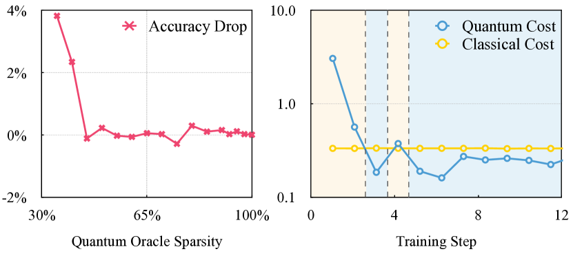
Figure 1: Left: As the oracle sparsity of the Hessian matrices decreases, there is no noticeable decline in accuracy compared to the results achieved using Newton’s GD (Gradient Descent) method with full Hessian matrices until a low threshold (around $40\%$). Right: While training with Newton’s GD, neither quantum nor classical methods consistently win in terms of inversion cost efficiency. Q-Newton strategically alternating between quantum and classical techniques for Hessian inversion tasks at each step.

Recent advancements in the literature highlight stochastic first-order optimization as the principal tool for training neural networks, predominantly due to its affordable computational expense. Its training cost scales linearly with that of its inference, making it an acceptable choice. In contrast, second-order methods, which could potentially offer a faster convergence rate, have garnered less attention. This is primarily due to their significant computational demands per iteration, with not only the computation of the Hessian but also its subsequent inversion. Specifically, the computing complexity for Hessian inversion grows cubically with the increase in the number of parameters, rendering them unscalable and impractical for neural networks lying in high-dimensional spaces.

Quantum linear solver algorithms (QLSAs) emerge as a potentially effective approach for addressing this challenge. Initially, the task of matrix inversion is reformulated into solving a set of linear equations, as inverting a matrix essentially entails determining a specific group of vectors that, when multiplied with the original matrix, yield the identity matrix. Specifically, for inverting a matrix of dimensions $N\times N$, QLSAs offer a quantum-state solution with a time complexity of $\mathcal{O}(d\cdot\kappa\log(N\cdot\kappa/\varepsilon))$. Here, {$d$, $\kappa$, $\varepsilon$} respectively represent the quantum oracle sparsity, condition number, and error tolerance. In contrast to the $\mathcal{O}(N^{3})$ time complexity of classical inversion methods, QLSAs hold the potential for an exponential speedup, making them a promising solution for the computationally intensive tasks during neural network training with Newton’s GD (Gradient Descent). However, this advantage is not universally applicable; as the complexity formula suggests, factors such as higher quantum oracle sparsity or a larger condition number can impact the efficiency gains offered by QLSAs. For example, a $10^{4}\times 10^{4}$ dense matrix with $\kappa$ of $10^{4}$ cannot be inverted more efficiently using QLSAs compared to classical solvers in our experiments.

To tackle these challenges, we propose a novel hybrid quantum-classical scheduling for accelerating neural network training with Newton’s gradient descent (Q-Newton). In each iteration of training, Q-Newton estimates and compares the computational expenses of quantum v.s. classical matrix inversion solvers, based on the given Hessian and gradient matrices. It then judiciously allocates the Hessian inversion task to whichever solver (quantum or classical) is supposed to be more cost-efficient. To streamline this process, Q-Newton incorporates a set of approximation and regularization techniques, significantly improving the overall scheduling efficiency and reducing runtime overhead.

Additionally, Q-Newton strategically defers the implementation of Newton’s GD to the later stages of training, motivated by certain characteristic observations during the initial training phase. Notably, we found that the Hessian matrix at the early stage typically exhibits ill-conditioned and is less sparse. These two attributes pose challenges for the effective application of Q-Newton: ① high condition number and less quantum oracle sparsity can severely limit the ability of quantum solvers to expedite matrix inversion, and ② high condition number often correlates with numerical instability, which can result in unreliable results during optimization.

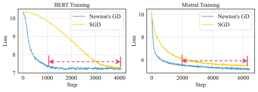
Figure 2: Training loss curves of Newton’s GD v.s. SGD (Stochastic Gradient Descent). The left is the training curve of a BERT model, and the right is the training loss curve of a Mistral model. Both are trained on the WikiText dataset from scratch. Newton’s GD demonstrates superiority on convergence compared to SGD, saving much training steps, i.e. $75\%$ for BERT and $67\%$ for Mistral.

In summary, we propose Q-Newton, targeting seamlessly coordinating between quantum and classical inversion solver for neural network training with Newton’s gradient descent, consisting of three crucial components as depicted below:

① A robust and lightweight Hessian condition number $\kappa$ estimator.

② A magnitude-based symmetry-aware pruning method designed to build quantum oracle sparsity in Hessian.

③ A Hessian regularization technique that lowers its condition number $\kappa$ to reduce time cost.

④ A plug-and-play scheduler for Hessian inversion tasks in Newton’s gradient descent training process.

Key results and insights are:

① Q-Newton demonstrates superiority over first-order optimizer (e.g., SGD, Stochastic Gradient Descent), as well as purely classical and quantum versions of Newton’s gradient descent.

② The Hessian in Q-Newton can be highly sparse while maintaining nearly the same performance, resulting in a significant reduction in time cost by over $90\%$.

③ Q-Newton Hessian regularization offers a trade-off between time cost and performance. Our experiments reveal the existence of an optimal trade-off, where we can reduce the condition number by a factor of $10^{3}$ with nearly no decrease in performance.

II Background

II-A Classic Optimizer for Network Training

Stochastic gradient descent (SGD) and its variants are the most used optimization algorithms for training neural networks [1, 2]. Central to SGD is the iterative update of the neural network parameters $\bm{\theta}$ towards minimizing the cost function $\mathcal{J}(\bm{\theta})$. This is achieved through the update rule $\bm{\theta}^{*}=\bm{\theta}_{0}-\alpha\nabla_{\bm{\theta}}\mathcal{J}$, where $\alpha$ is the learning rate, $\bm{\theta}_{0}$ is the initial parameter set, and $\nabla{\bm{\theta}}\mathcal{J}$ is the gradient of the cost function with respect to $\bm{\theta}$. In each iteration, SGD selects a mini-batch of data, computes the gradient $\nabla{\bm{\theta}}\mathcal{J}$ on this batch, and adjusts $\bm{\theta}$ accordingly. Variants of SGD, such as SGD with momentum and adaptive learning rate methods, are built upon this fundamental principle and sometimes aim to approximate second-order information. They introduce mechanisms that not only accelerate convergence but also stabilize the update process [3, 4]. By emulating aspects of second-order optimization methods, these enhancements potentially improve the efficiency and robustness of SGD.

Nevertheless, to achieve faster convergence with satisfactory generalization properties in these domains is often laden with numerous ad-hoc rules that must be followed precisely. Even the first-order optimizer selection, which has become a rule of thumb, critically influences performance outcomes. For instance, in computer vision field, SGD with momentum is the preferred choice [5]; whereas, in natural language processing area, Adam [3] and AdamW [4] are more commonly employed for training transformer models [6, 7, 8].

II-B Second-order Optimizer - Newton’s Gradient Descent

Second-order optimization techniques are among the most powerful methods developed for optimization, with several implementations aimed at enhancing the training of neural networks [1]. These methods effectively rescale gradients in order to tackle ill-conditioned optimization challenges. They improves the direction of parameter update and facilitates an adaptive learning rate for each parameter. Numerous theoretical analyses have demonstrated the superior convergence rates achieved by methods based on second-order optimization.

Newton’s GD, one of the classical second-order approaches, employs a second-order Taylor series expansion for approximating the objective function $\mathcal{J}(\bm{\theta})$ around a reference point $\bm{\theta}_{0}$. This approximation is formulated as:

$$\mathcal{J}(\bm{\theta})\approx\mathcal{J}(\bm{\theta}_{0})+(\bm{\theta}-\bm{\theta}_{0})^{\text{T}}\nabla{\bm{\theta}}\mathcal{J}(\bm{\theta}_{0})+\frac{1}{2}(\bm{\theta}-\bm{\theta}_{0})^{\text{T}}\mathtt{H}(\bm{\theta}-\bm{\theta}_{0}),$$

where $\mathtt{H}$ represents the Hessian matrix of $\mathcal{J}$ with respect to $\bm{\theta}$ at $\bm{\theta}_{0}$. It then leads to the Newton parameter update rule:

$$\bm{\theta}^{*}=\bm{\theta}_{0}-\mathtt{H}^{-1}\nabla_{\bm{\theta}}\mathcal{J}$$

Iteratively applying this update, akin to the update rule of SGD introduced in Section II-A, leads to the algorithm detailed in Algorithm 1.

Algorithm 1 Newton’s GD for objective $\mathcal{J}(\bm{\theta})$

0:  Learning rate $\beta$

0:  Initial parameter $\bm{\theta}_{0}$

0:  Training set of $m$ examples

1:  Objective $\mathcal{J}(\bm{\theta})=\frac{1}{m}\sum_{i=1}^{m}\mathcal{L}\left(f(\bm{x}^{(i)};\bm{\theta}),\bm{y}^{(i)}\right)$

2:  while stopping criterion not met do

3:     Compute gradient: $\bm{g}\leftarrow\frac{1}{m}\nabla_{\bm{\theta}}\sum_{i}\mathcal{L}\left(f(\bm{x}^{(i)};\bm{\theta}),\bm{y}^{(i)}\right)$

4:     Compute Hessian: $\mathtt{H}\leftarrow\frac{1}{m}\nabla_{\bm{\theta}}^{2}\sum_{i}\mathcal{L}\left(f(\bm{x}^{(i)};\bm{\theta}),\bm{y}^{(i)}\right)$

5:     Compute Hessian inverse: $\mathtt{H}^{-1}$

6:     Compute update: $\Delta\bm{\theta}=-\mathtt{H}^{-1}\bm{g}$

7:     Apply update: $\bm{\theta}=\bm{\theta}+\beta\cdot\Delta\bm{\theta}$

8:  end while

Challenge $1$ - Ill-posed Hessian. It is important to note that Newton’s GD is suitable primarily when the Hessian is positive definite. In the realm of neural network training, the landscape of the objective function typically exhibits non-convex characteristics, marked by various complexities like saddle points [1]. These features can pose challenges for Newton’s GD. For instance, in the vicinity of a saddle point, if the Hessian’s eigenvalues are not all positive, Newton’s method may inadvertently guide updates in an undesirable direction. To overcome such issues, a common solution includes the Hessian regularization. One widely used regularization technique is adding a constant $\alpha$ to the Hessian’s diagonal, resulting in a modified, regularized Hessian of the form $(\mathtt{H}+\alpha\mathtt{I})$.

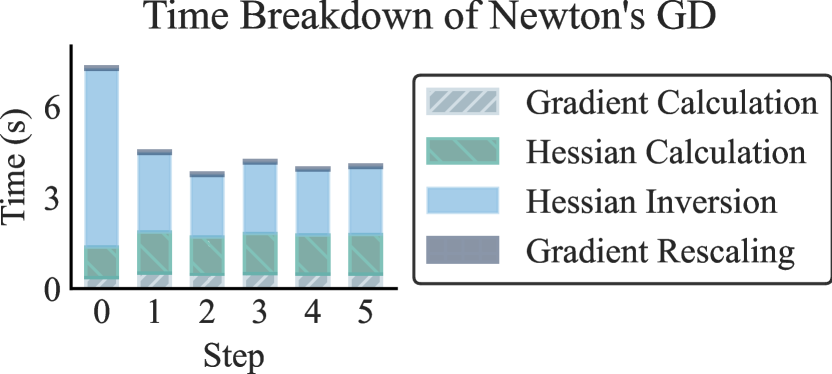
Figure 3: The execution time breakdown across various initial steps in the DNN model training with purely classical Newton’s GD, which focuses on four dominant stages including gradient & Hessian calculation, Hessian inversion and gradient rescaling.

Challenge $2$ - Massive Cost for Computing Hessian. Newton’s GD, in contrast to SGD, incurs substantial extra computational costs, mainly due to ① the computation of Hessian, and ② its inversion, as illustrated in Algorithm 1. Our profiling of Newton’s gradient descent’s execution time, as depicted in Figure 3, demonstrates that inverting the Hessian matrix constitutes the main computational bottleneck. To address this challenge, our work focuses on leveraging quantum linear solver algorithms to effectively mitigate this overhead.

II-C Matrix Inversion Solvers in Classical Machines

Definition of Matrix Inversion. The matrix $\mathtt{A}$ is a square matrix of shape $N\times N$. The inverse of $\mathtt{A}$ is another square matrix, denoted by $\mathtt{A}^{-1}$, such that $\mathtt{A}\mathtt{A}^{-1}=\mathtt{A}^{-1}\mathtt{A}=\mathtt{I}_{N}$, where $\mathtt{I}_{N}$ is the identity matrix of order $N$.

In classical computers, the inverse of a matrix can be computed using many methods [9], such as Gauss-Jordan elimination, LU decomposition [10], singular value decomposition (SVD) [11]. Among these, LU decomposition is predominantly used in modern computers, finding applications in numerical libraries and software such as LAPACK [12]. Its widespread use is attributed to its optimal operational count, ease of parallelization [13], and a well-balanced trade-off between computational efficiency and numerical stability. In line with these advantages, our research adopts LU decomposition as the go-to algorithm for classical matrix inversion solving. LU decomposition has a time complexity of $\Theta(N^{3})$ for an $N\times N$ matrix.

II-D Matrix Inversion Solvers in Quantum Machines

QLSAs can be used to solve matrix inversion. In QLSAs, the solution to a linear system represented by $\mathtt{A}\bm{x}=\bm{b}$ is encoded into a quantum state. Precisely, given an error tolerance $\varepsilon$, QLSs produce a quantum state $|\hat{\bm{x}}\rangle$ so that $|\bm{x}\rangle=\frac{\mathtt{A}^{-1}|\bm{b}\rangle}{\|\mathtt{A}^{-1}|\bm{b}\rangle\|}$ and $\||\hat{\bm{x}}\rangle\ -|\bm{x}\rangle\ \|\leq\varepsilon$. It is important to note that $|\bm{x}\rangle$ is a normalized solution and the normalization constant $\|\mathtt{A}^{-1}|\bm{b}\rangle\|$ must be determined separately. Additionally, vector $\bm{b}$ is assumed to be normalized, allowing it to be stored in a quantum state.

Overview of QLSA. According to the original implementation [14], the algorithms begin with the eigen-decomposition of the matrix $\mathtt{A}$, represented in the quantum domain using Hamiltonian simulation as $U=e^{i2\pi\mathtt{A}}$. Then the Quantum Phase Estimation (QPE) process maps each eigenstate of $\mathtt{A}$ to its corresponding eigenvalue, encoding this information in an ancillary quantum register. This is pivotal for the next stage, the Controlled Rotation (CR), where the algorithm uses the eigenvalues in the ancilla register to apply the operation $1/\lambda_{j}$ on each component of the quantum state, effectively inverting the matrix $\mathtt{A}$. The final step is the Inverse QPE. Here, the algorithm reverts the ancilla register to its initial state and measures it, collapsing the system into a state that approximates the solution $|\bm{x}\rangle$. However, this state is unnormalized, and an additional step is required to estimate the normalization constant. This is achieved by repeatedly running the circuit and measuring the probability of obtaining specific quantum states, from which the normalization constant can be deduced. The entire quantum circuit is shown in Figure 4.

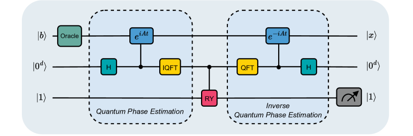
Figure 4: Schematic of the QLSA circuit flowing from left to right.

The running cost of QLSAs depends significantly on certain properties of the matrix $\mathtt{A}$, such as quantum oracle sparsity, condition number and the precision of quantum operations. This is because, sparse matrices and lower condition numbers ease the eigen-decomposition and Hamiltonian simulation, while the precision in quantum operations directly impacts the accuracy and efficiency of the algorithm. Details of the running cost are illustrated in Section II-E.

QLSAs for Matrix Inversion. Linear solver algorithms can be effectively employed for computing the inverse of a matrix $\mathtt{W}$. Specifically, the $i$th column of $\mathtt{W}^{-1}$ can be obtained by solving the linear equation $\mathtt{W}\bm{x}_{i}=\bm{e}_{i}$, where $\bm{e}_{i}$ represents a one-hot column vector with its $i$th element set to $1$. By assembling all such columns, the matrix inversion problem for $\mathtt{W}$ can be elegantly formulated as:

$$\begin{pmatrix}\mathtt{W}&0&\cdots&0\\ 0&\mathtt{W}&\cdots&0\\ \vdots&\vdots&\ddots&\vdots\\ 0&0&\cdots&\mathtt{W}\end{pmatrix}\cdot\mathtt{X}=\begin{pmatrix}\bm{e}_{1}\\ \bm{e}_{2}\\ \vdots\\ \bm{e}_{N}\end{pmatrix},$$ (1)

where $\mathtt{X}$ is a flattened vector representing the solution of $\mathtt{W}^{-1}$.

II-E Running Costs of Quantum Linear Solvers

Unlike many classical linear solver algorithms, QLSAs have a time complexity influenced by a variety of factors beyond just the size of the matrix [14]. Consider solving a system of linear equations $\mathtt{A}\bm{x}=\bm{b}$, where $\mathtt{A}$ is a $N\times N$ matrix. The running cost of QLSAs in solving this problem is determined not only by ① the size of the matrix $N$, but also by ② the matrix’s condition number $\kappa$, ③ the quantum oracle sparsity $d$ of the matrix, and ④ the desired error tolerance $\varepsilon$.

Time Complexity. Since the first QLSA by Harrow, Hassidim, and Lloyd (HHL) [14] that exhibits a complexity of $\mathcal{O}\left(d\kappa^{2}/\varepsilon\log{N}\right)$, there has been a significant number of works aimed at reducing this original complexity. For instance, researchers [15] employed quantum signal processing (QSP) techniques to devise an algorithm with $\mathcal{O}(\kappa\mathrm{polylog}(\kappa/\varepsilon))$ complexity. While these advancements highlight the potential of quantum algorithms, a comprehensive analysis detailing the explicit query counts remains unexplored, and the existing analytical bounds for constant prefactors yield exceedingly high numbers.

Explicit Query Counts. Recent advancements, notably by [16], have yielded significant progress with a closed-form expression for the non-asymptotic query complexity of QLSAs. This formula, denoted as $\mathcal{Q}^{*}(N,\kappa,d,\varepsilon)$, explicitly determines the number of queries required for block-encoding the linear system matrix. This advancement allows for a more precise estimation of the latency overhead in QLSAs. Firstly, considering the success probability is bounded below by $(0.39-0.201\varepsilon)$, where $\varepsilon$ represents the error tolerance, the expected query complexity, factoring in the possibility of failure, is calculated as $\left(\frac{\mathcal{Q}^{*}}{0.39-0.201\varepsilon}\right)$. Secondly, to accurately gauge the real-time execution duration of each query, we can refer to either calibration statistics from actual quantum platforms like IBM Quantum or a promised gate time, providing a realistic perspective on the operational time cost. Moreover, currently one of the fastest quantum gate processors could be made using photonic based quantum computing, which could potentially improve the gate time towards GHz ($10^{-9}$s), THz ($10^{-12}$s) and further [17, 18]. It is also possible that in the future the quantum gate speed is possibly improved by attosecond physics [19, 20], towards a possible gate time of few attoseconds ($10^{-18}$s). Therefore, we can achieve a comprehensive understanding of the time cost of Q-Newton.

Qubit Cost. Alongside the analysis of time requirements, the study by [16] also presents the qubit requirements for QLSAs, offering a clear formula for space costs. This is represented as $\left(a+6+\lceil\log_{2}N\rceil\right)$ logical qubits. The variable $a$, influenced by the block-encoding of the matrix, is bounded at a minimum by the error tolerance $\varepsilon$. This precise formula helps in assessing the quantum hardware resources needed for implementing QLSAs.

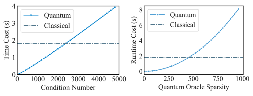
Figure 5: The scaling curves of time cost for classical and quantum solvers to condition number (left) and quantum oracle sparsity (right). The condition number scaling curve is calculated at a fixed sparsity $1000$, and the sparsity scaling curve is calculated at a fixed condition number $10000$.

III Motivation: Q-Newton for NN Training

In this section, we introduce the insights behind our quantum-classical scheduling design, including the runtime overhead of quantum & classical matrix inversion solvers, and the evolution of Hessian matrices throughout the neural network training process with Newton’s gradient descent.

III-A Why Needs Newton’s GDs?

A: Better convergence. Newton’s GD, as a classical second-order method, can improve the direction of gradient descent and facilitates an adaptive learning rate for each parameter. Numerous theoretical analyses have demonstrated the superior convergence rates achieved by methods based on second-order optimization. Our experiments also demonstrate, as shown in Figure 2, Newton’s GD brings up to $4\times$ the convergence acceleration compared to SGD in terms of training steps.

III-B Always Quantum Inversion Solvers?

A: No. A trade-off exists between classical & quantum solvers.

Classical Solvers. As illustrated in Figure 5, a notable characteristic of classical solvers, especially the LU decomposition method, is their consistently high computational cost, which primarily depends on the matrix size and remains largely unaffected by other specific attributes of the matrix. This characteristic is particularly relevant in our context of neural network training with Newton’s GD. While the left side of Figure 2 indicates that Newton’s GD may necessitate fewer training iterations, this doesn’t translate to a corresponding decrease in overall training time with classical inversion solvers; in fact, it may even lead to an increase. This is primarily because each iteration in Newton’s GD involves solving matrix inversion, which becomes increasingly time-consuming for larger matrices. Consequently, even with fewer iterations, the cumulative time taken for these computationally intensive operations results in a training process that is still too prolonged to be practical for training non-trivial neural networks.

Quantum Solvers. In contrast to their classical counterparts, the computational costs of quantum inversion solvers are not consistently tied to the size of the matrix. As discussed in Section II-E, these costs are associated with additional matrix properties, such as quantum oracle sparsity $d$ and condition number $\kappa$. This correlation renders quantum solvers exceptionally efficient when these parameters fall below certain thresholds, as depicted in Figure 5. Notably, in the context of neural network training using Newton’s GD, the characteristics of the Hessian matrix evolve, leading to fluctuations in the computational demands of its inversion when tackled with quantum inversion solvers.

Consequently, employing a classical inversion solver consistently throughout the training process for all Hessian matrices results in a persistently high and often prohibitive total runtime cost. This is the case even though the total number of training steps might be fewer. On the other hand, while quantum inversion solvers can offer substantial speed-ups for matrices with lower quantum oracle sparsity or favorable condition numbers, their performance can significantly deteriorate for matrices that do not exhibit these advantageous properties.

III-C What are Beneficial Hessian Dynamics?

A: The sparsity and condition number of Hessian.

Hessian Sparsity. Numerous studies [21, 22] have discovered that, in the initial stages of neural network training, the Hessian matrix of the network exhibits a broad range of large positive and negative eigenvalues, resulting in large condition number. However, this scenario changes rapidly after a few training steps: a small number of large eigenvalues begin to dominate, most eigenvalues hover around zero, and the negative eigenvalues shrink significantly. Essentially, the eigenvalues of the Hessian matrix exhibit a trend towards ”sparsity” as training progresses.

Building on this observation, our work explores a similar pattern of ”sparsity” in the magnitude distribution of the Hessian matrix rows. We conduct an empirical analysis focusing on the $p\%$ quantum oracle sparsity ($p\%$-sparsity) for each Hessian row at different stages of training. Specifically, for a given row of the Hessian, we determine the smallest subset of its elements that add up for $p\%$ of the total absolute value of the row, with the size of this subset being the $p\%$-sparsity. The results, as depicted in Figure 6, clearly indicate a trend of decreasing quantum oracle sparsity over the course of training.

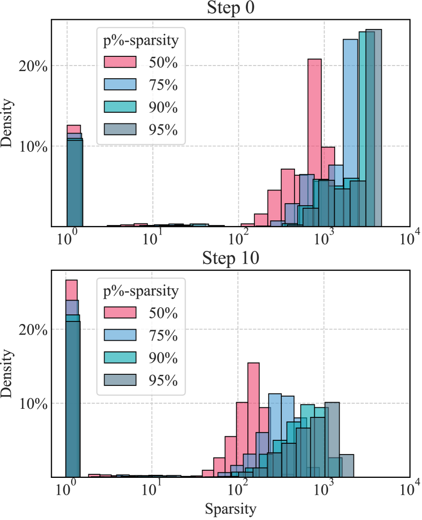
Figure 6: The distribution of $p\%$ quantum oracle sparsity ($p\%$-sparsity) for each row of the Hessian matrix at two distinct points in the training process: step $0$ (up) and step $10$ (down). The $p\%$-sparsity metric is defined as the fewest number of elements in a given row that, when added together, contribute to $p\%$ of the row’s total absolute magnitude. These distributions were obtained during the training of the DNN model on the MNIST dataset, with Hessian matrix of shape $12544\times 12544$, providing insights into the evolving magnitude distribution within the Hessian matrix as training progresses. We evaluate the $p\%$ across $\{50\%,75\%,90\%,95\%\}$.

Hessian Condition Number. During the iterative updating of neural network parameters in the training process, there is a notable shift in the local structure of the loss function. This evolution is characterized by the loss function becoming more ”flat”, particularly as the network nears its optimal configuration [23]. Such flattening affects the condition number of the Hessian matrix, generally causing it to decrease. As the loss function becomes flatter, the magnitudes of its second-order derivatives diminish, indicating a reduction in the function’s curvature in any direction. This results in a corresponding decline in the eigenvalues of the Hessian matrix. The condition number, defined as the ratio of the largest to the smallest non-zero eigenvalue of the Hessian, consequently diminishes as training progresses. This trend mirrors the transformation of the loss function within the parameter space, moving from an initially steep curvature to a progressively gentler landscape.

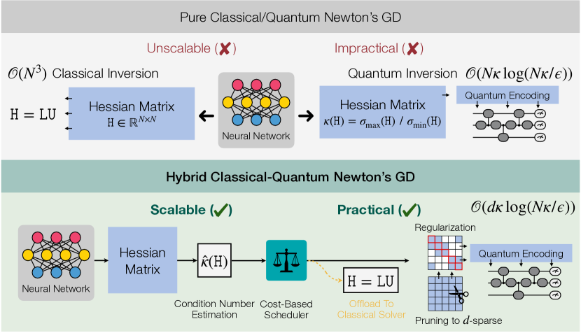
Figure 7: Overview of Q-Newton. Both purely classical and quantum Newton’s GD are unscalable and impractical. Purely classical Newton’s GD calculates the Hessian inversion via LU decomposition etc., with a time complexity of $\mathcal{O}(N^{3})$. Quantum Newton’s GD requires substantial time when the Hessian is either ill-conditioned or non-sparse. Hybrid classical-quantum Newton’s GD adaptively schedules between classical and quantum inversion solvers, and incorporates pruning and regularization techniques, making it scalability and practicality.

IV Adaptive Quantum-Classical Scheduler

To facilitate efficient Newton’s GD for accelerating neural network training, we propose Q-Newton, a hybrid quantum-classical scheduling for accelerating neural network training with Newton’s gradient descent. Q-Newton works by estimating the running costs associated with both quantum and classical solvers when inverting Hessian matrices and then allocating the task to the more efficient solver. This section outlines Q-Newton, including the detailed algorithm used for estimating cost and reducing cost.

IV-A Overview of Q-Newton

Generally, each iteration of Newton’s GD typically unfolds across five distinct execution stages: ① forward & backward propagation involves processing the input data, calculating the loss, and computing gradients for each parameter; ② Hessian propagation is responsible for computing the Hessian matrices; ③ Hessian inversion deals with inverting these Hessian matrices; ④ gradient rescaling entails multiplying the inverse of the Hessian with the gradient to rescale it; ⑤ parameter update applies these rescaled gradients following the stochastic gradient descent update rule. In our Q-Newton, the focus is on strategically scheduling the ④ gradient rescaling and ⑤ parameter update stages between quantum and classical solvers, while the remaining stages are executed on classical processors. Figure 7 provides a schematic of the Q-Newton framework compared to purely classical and quantum approach, where a scheduler strategically assigns the gradient and Hessian to either quantum or classical solvers for efficient gradient rescaling, making it scalable and practical.

IV-B Early Phase without Newton’s GD

The insight #1 in Section III-B highlights that quantum linear solvers are poised for speed advantages over classical counterparts predominantly when dealing with matrices characterized by low condition number and quantum oracle sparsity. However, this ideal scenario is not universally applicable. As elucidated by the insight #2 #3 in Section III-C, during the initial stages of neural network training, both the condition number and quantum oracle sparsity tend to be considerably high, presenting a dual challenge to our approach:

• Efficiency-driven Concerns: The presence of high condition number and quantum oracle sparsity in matrices can significantly impede the quantum solvers’ ability to accelerate matrix inversion processes.

• Effectiveness-driven Concerns: A higher condition number often implies a matrix nearing singularity, which can result in its inverse being numerically unstable. This instability potentially leads to erratic outcomes in iterative computations.

Given these two considerations, Q-Newton employs only first-order training methods (i.e. SGD) during the early phase of training.

Algorithm 2 Overall procedure of Q-Newton.

0:  Classical benchmarked constant factor $C$

0:  Quantum average gate time $t_{\text{g}}$

0:  Learning rate $\beta$

0:  Initial parameter $\bm{\theta}_{0}$

0:  Training set of $m$ examples

1:  Objective $\mathcal{J}(\bm{\theta})=\frac{1}{m}\sum_{i=1}^{m}\mathcal{L}\left(f(\bm{x}^{(i)};\bm{\theta}),\bm{y}^{(i)}\right)$

2:  while stopping criterion not met do

3:     Compute gradient: $\bm{g}\leftarrow\frac{1}{m}\nabla_{\bm{\theta}}\sum_{i}\mathcal{L}\left(f(\bm{x}^{(i)};\bm{\theta}),\bm{y}^{(i)}\right)$

4:     Compute Hessian: $\mathtt{H}\leftarrow\frac{1}{m}\nabla_{\bm{\theta}}^{2}\sum_{i}\mathcal{L}\left(f(\bm{x}^{(i)};\bm{\theta}),\bm{y}^{(i)}\right)$

5:     Estimate classical cost: $\mathcal{R}_{\text{c}}=C\cdot N^{3}$

6:     Estimate quantum cost: $\mathcal{R}_{\text{q}}=t_{\text{g}}\cdot\mathcal{Q}(\mathtt{H})$

7:     if $\mathcal{R}_{\text{c}}<\mathcal{R}_{\text{q}}$ then

8:        Solve classical matrix inversion: $\mathtt{H}^{-1}=\mathrm{LUInv}(\mathtt{H})$

9:        Compute update: $\Delta\bm{\theta}=-\mathtt{H}^{-1}\bm{g}$

10:     else

11:        Encode quantum Hessian: $\mathtt{H}=\mathrm{QEncode}(\mathtt{H})$

12:        Solve quantum matrix inversion: $\mathtt{H}^{-1}=\mathrm{QLSA}(\mathtt{H})$

13:        Encoding quantum gradient: $\bm{g}=\mathrm{QEncode}(\bm{g})$

14:        Compute update in circuit: $\Delta\bm{\theta}=-\mathtt{H}^{-1}\bm{g}$

15:        Decode quantum update: $\Delta\bm{\theta}=\mathrm{QDecode}(\Delta\bm{\theta})$

16:     end if

17:     Apply update: $\bm{\theta}=\bm{\theta}+\beta\cdot\Delta\bm{\theta}$

18:  end while

IV-C Scheduling via Costs Estimation

When provided with a Hessian and gradient pair $(\mathtt{H},\bm{g})$, the Q-Newton scheduler initially calculates the estimated costs of inverting the Hessian using both quantum and classical solvers. Subsequently, it allocates the Hessian inversion task to the solver with the lower runtime costs. In this section, we present the algorithms used for this running cost estimation.

Classical Solver Cost Estimation. The classical solver employs LU decomposition with a time complexity of $\Theta(N^{3})$. To estimate its runtime cost, we represent it as $\mathcal{R}_{\text{c}}=C\cdot N^{3}$, where $C$ is a constant factor that can be easily determined through a benchmark calibration on different platforms.

Quantum Solver Cost Estimation. Building on the discussion in Section II-E, the study by [16] offers a closed-form expression for the query complexity of QLSAs, denoted as $\mathcal{Q}(N,\kappa,d,\varepsilon)$. To estimate the total running cost $\mathcal{R}{\text{q}}$ for quantum solvers, we use a gate time of $10^{-18}$s. Though beyond current quantum techniques, it is possibly realised by the attoseconds physics in the future [19, 20].

To streamline this cost estimation in Q-Newton, several approximation strategies are employed. Firstly, instead of requiring an exact condition number $\kappa$, an upper bound is used as per [16]. We calculate this upper bound following the approach by [24], which only necessitates computing the matrix’s determinant and trace, thereby enhancing efficiency. Secondly, given that Hessian matrices are not typically sparse, we approximate by selecting the top contributing values, cumulatively accounting for $50\%$ of the total absolute value in each row. This approximation approach maintains the accuracy of the Hessian inverse, particularly when the condition number is small in the later training phases, aligning with our insights in Section IV-B. The details of this sparsifying process for Hessian matrices are further elaborated in Section IV-D. Thirdly, drawing from the successful application of low precision in deep learning [25, 26], a relatively low error tolerance $\varepsilon$, specifically $10^{-12}$, is deemed sufficient in Q-Newton.

IV-D Sparsifying Hessian Matrix

Q-Newton employs a pruning strategy to obtain a pruned Hessian matrix with quantum oracle sparsity, which involves selecting the most significant values while discarding the rest. Intuitively, this pruning approach does not introduce substantial errors in the inverse matrix when the condition number of the Hessian is low. This can be understood considering that, in a linear system $\mathtt{A}\bm{x}=\bm{b}$, the condition number of $\mathtt{A}$ is essentially indicative of how sensitive the solution $\bm{x}$ is to changes in $\bm{b}$. Therefore, when the condition number of $\mathtt{H}$ is small, minor inaccuracies in $\mathtt{H}$ are less likely to lead to significant errors in solving the equation $\mathtt{H}\bm{x}=\bm{e}_{i}$, where $\bm{x}$ represents the $i$th column of $\mathtt{H}^{-1}$.

QLSAs, when applied to matrix inversion problems, necessitate the matrix being Hermitian. Fortuitously, Hessian matrices inherently fulfill this condition. However, a straightforward row pruning approach, which selects the top values independently for each row, could disrupt this Hermitian property. To circumvent this issue, we introduce a symmetry-aware pruning method aimed at retaining the $d$ quantum oracle sparsity. Our approach, implemented in Q-Newton, involves initially sorting all elements in the Hessian matrix and systematically selecting from the largest, ensuring that corresponding symmetrical elements are chosen simultaneously. Once a row or column accumulates up to $d$ selected elements, it is then excluded from further selection. This procedure effectively preserves the matrix’s symmetry throughout the pruning process.

IV-E Streamlined Gradient Rescaling within Quantum Circuits

It’s important to note that QLSAs provide the solution in the form of a quantum state. Attempting to extract the entire inverse Hessian matrix $\mathtt{H}^{-1}$ would be an intensive task, potentially diminishing the time complexity benefits that QLSAs have over traditional classical solvers. To address this, Q-Newton employs a strategy where the gradient vector $\bm{g}$ is encoded into quantum states. The rescaled gradient $\mathtt{H}^{-1}\bm{g}$ is then efficiently computed using enhanced quantum circuits, a process facilitated by the widely-used SWAP test technique, as described in [27]. In the final step, Q-Newton directly reads out the rescaled gradient, which is then used for subsequent updates of the parameters.

V Evaluation

V-A Evaluation Setup

In our evaluation, we compare Q-Newton with two baseline approaches: Classical Solver Only and Quantum Solver Only, which serve as benchmarks for scenarios where our scheduling technique is not applied. Our experiments involve training three distinct and representative models, {DNN, BERT [6]  Mistral [28]}, on two datasets: {MNIST [29], WikiText [30]}. These datasets span two key areas in deep learning: computer vision and natural language processing. A summary of the models used is presented in Table I. For the DNN model, we calculate the exact Hessian for all parameters, leveraging its relatively smaller size. However, for the larger model, i.e. BERT and Mistral, we resort to approximated layer-wise Hessian computation using the empirical Fisher method [31], as their extensive parameter count renders the computation of exact Hessian impractical. For a better start point, we initialize the embedding layers in our BERT and Mistral model from the pre-trained BERT-base and Mistral-7B with PCA down projection. We apply batch size $2048$ for DNN model, $128$ for BERT and Mistral, as these are the largest batch sizes that can be accommodated by a single H100 GPU with 80GB of memory.

TABLE I: Summary of neural networks for evaluation.

Architecture	Hidden Dimension	Layers	Number of Parameters
DNN	$16$	$2$	$13$K
BERT [6]	$64$	$4$	$2.2$M
Mistral [28]	$64$	$4$	$4.3$M

TABLE II: Execution time of condition number estimation for matrices with different sizes $N\times N$.

Size ($N$)	$10$	$10^{2}$	$10^{3}$	$10^{4}$
Time (ms)	$0.1$	$0.7$	$6.2$	$13.0$

Platform For our experiments, the classical computations were carried out on the NVIDIA H100, while the quantum computational aspects utilized calibration data from IBM Quantum’s ibm_sherbrooke quantum machine. On the classical side, our experiments were conducted using JAX and PyTorch frameworks.

Extra Runtime Overhead The main source of additional runtime introduced in our Q-Newton approach arises from the time needed to estimate the condition number and read out the rescaled gradient vector from the quantum state. This section presents an analysis of the condition number estimation’s runtime overhead across various matrix sizes. The results, detailed in Table II, reveal that the execution time for this phase is inconsequential.

V-B Comparison Against Baselines

Our evaluation encompassed the per-step execution time and the total number of training steps for three distinct approaches: {Q-Newton, Classical Solver Only, Quantum Solver Only}, applied within the context of Newton’s gradient descent. Additionally, we assessed the performance of first-order optimizer, SGD, without incorporating Newton’s GD. The detailed results are presented in Table III, Table IV. We use the quantum gate time of $10^{-18}$s. We use regularization coefficient $1.0$ and $0.5$ for DNN and Mistral separately, as they are empirically optimal in terms of performance.

TABLE III: Summary of training runtime evaluation results of the DNN model on the MNIST dataset. Note that Newton’s GD exhibits better convergence, requiring fewer training steps to achieve the same performance compared to SGD.

Method	Total Steps	Time Per Step	Total Time
SGD	$1500$	$0.14$s	$204$s
Classical-Only	$1000$	$1.06$s	$1064$s
Quantum-Only	$1000$	$0.17$s	$170$s
Q-Newton	$1000$	$0.15$s	$\mathbf{123}$s

TABLE IV: Summary of training runtime evaluation results of the Mistral model on the WikiText dataset. Note that Newton’s GD exhibits better convergence, requiring fewer training steps to achieve the same performance compared to SGD.

Method	Total Steps	Time Per Step	Total Time
SGD	$6200$	$0.1$s	$11.1$min
Classical-Only	$2000$	$9.8$s	$334.2$min
Quantum-Only	$2000$	$0.1$s	$3.8$min
Q-Newton	$2000$	$0.1$s	3.5min

V-C Trade-off Between Sparsity and Performance

To evaluate the impact of sparse Hessian matrices arising from pruning, we executed experiments by varying the sparsity levels of the quantum oracle and observing the consequent performance degradation in DNN training. As depicted on the left side of Figure 1, it demonstates that performance remains relatively stable with only a minimal decline when sparsity exceeds $40\%$.

V-D Trade-Off Between Condition Number and Performance

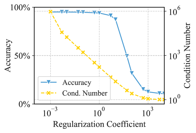
Figure 8: The performance and condition number trade-off curve when varying the Hessian regularization coefficient. The optimal trade-off is achieved when the regularization coefficient is around $1$.

The Hessian is sometimes ill-conditioned, which poses challenges for efficient quantum matrix inversion solvers. To address this issue, we further regularize the Hessian and explore the trade-off between performance and the time cost (i.e., the condition number factor). Specifically, given a regularization coefficient $\epsilon$, we compute the regularized Hessian matrix $\mathtt{H}_{\text{reg}}\in\mathbb{R}^{N\times N}$ as follows:

$$\mathtt{H}_{\text{reg}}=\mathtt{H}+\epsilon*\mathtt{I},$$

where $\mathtt{I}\in\mathbb{R}^{N\times N}$ is the identity matrix. In Figure 8, we conduct ablation study on the DNN training on MNIST dataset,.. investigate the accuracy after training and the condition number as $\epsilon$ varies. The results demonstrate that we can decrease the condition number by $10^{3}$ times with only a marginal performance decrease when the regularization factor $\epsilon$ is around $1$.

VI Discussion and Future Work

VI-A QLSA Circuit Compilation

Our Q-Newton simulations are currently conducted using classical algorithms, and there remains an absence of practical implementation for running QLSA programs either in simulations or on actual quantum computers. Future efforts directed at refining quantum circuit compilation techniques hold promise for enhancing its performance. This will entail the creation of innovative algorithms or the improvement of existing ones to streamline the quantum circuit design, reduce the number of quantum gate operations, and lower the overall quantum error rates. Moreover, continually updating these compilation strategies to align with the rapid developments in quantum hardware technology will be essential.

VI-B Hessian Matrix Row-Spasification

In Q-Newton, the quantum oracle sparsity of the input matrix significantly enhances block-encoding efficiency, which in turn reduces the runtime cost of the entire QLSA. We strategically prune the Hessian matrix to achieve this quantum oracle sparsity, influenced by the observed pattern of sparsity in the magnitude distribution of the matrix’s rows. It’s noteworthy that the beneficial efficiency doesn’t solely rely on quantum oracle sparsity. Future research could also delve into the low-rank sparsity patterns observed in neural network Hessians post the initial phase, as discussed in [32]. The potential interaction between low-rank sparsity and efficient quantum block encoding forms a compelling subject for future exploration, as highlighted in recent studies like [33] and [34].

VI-C Saddle Points

In the scenario of neural network training, the landscape of the objective function is often nonconvex and features various topological characteristics, including saddle points. At these saddle points, the gradient is near zero. Typically, in the early stages of neural network training, the network finds itself in regions of high curvature within the parameter space. These areas are frequently populated with intricate saddle points, presenting significant challenges. Gradient descent methods, which depend solely on first-order derivative information, may falter in these regions due to the near-zero gradients encountered at saddle points [35]. In contrast, Newton’s GD, leveraging second-order derivative information (specifically, the Hessian matrix), can more adeptly maneuver around these saddle points. Therefore, as suggested by works like [36], employing Newton’s GD during the initial phase of training can be particularly advantageous in effectively navigating this complex terrain.

VII Related Work

Approximate Second-Order-Based Methods for Neural Network Training. In our Q-Newton approach, we leverage Newton’s gradient descent, which enhances optimization by utilizing second derivatives, encompassing the computation and inversion of the exact Hessian matrix. Alongside Newton’s GD, several other algorithms also employ the Hessian matrix in training [1]. Notably, Conjugate Gradient [37] efficiently circumvents the need to compute the inverse Hessian by iteratively descending along conjugate directions. This strategy emerges from an in-depth analysis of the shortcomings inherent in the method of steepest descent. Similarly, the Broyden–Fletcher–Goldfarb–Shanno (BFGS) [38, 39, 40, 41] algorithm aims to harness some benefits of Newton’s method but without its computational intensity. It iteratively refines an approximating matrix with low-rank updates, progressively honing it into a closer representation of the Hessian inverse. Furthermore, the BFGS algorithm’s memory demands can be substantially reduced by not retaining the full inverse Hessian approximation, thus giving rise to the L-BFGS algorithm [42], which is more memory-efficient.

VIII Conclusion

In this paper, we introduce Q-Newton, a novel hybrid quantum-classical scheduler designed to enhance the efficiency of neural network training using Newton’s GD. This approach effectively addresses the computational challenges of second-order optimization, particularly the intensive matrix inversion process. By integrating Quantum Linear Solver Algorithms (QLSAs), Q-Newton harnesses the potential of quantum computing for exponential acceleration in matrix inversion, crucial for Newton’s GD. Our Q-Newton adeptly balances the strengths and limitations of quantum computing, considering factors like the matrix’s condition number and quantum oracle sparsity. Moreover, Q-Newton includes several techniques to further reduce quantum time cost.

While Q-Newton shows promise in leveraging quantum algorithms for classical machine learning, future work that focuses on refining quantum circuit compilation techniques could further enhance its efficacy. This involves developing new algorithms or improving existing ones to optimize the quantum circuit layout, minimize quantum gate operations, and reduce overall quantum error rates. Additionally, adapting these compilation strategies to keep pace with the rapid advancements in quantum hardware will be crucial.

References

- [1] I. Goodfellow, Y. Bengio, and A. Courville, Deep Learning. MIT Press, 2016. http://www.deeplearningbook.org.
- [2] Q. V. Le, J. Ngiam, A. Coates, A. Lahiri, B. Prochnow, and A. Y. Ng, “On optimization methods for deep learning,” ICML’11, p. 265–272. Omnipress, Madison, WI, USA, 2011.
- [3] D. P. Kingma and J. Ba, “Adam: A method for stochastic optimization.” 2017.
- [4] I. Loshchilov and F. Hutter, “Decoupled weight decay regularization.” 2019.
- [5] K. He, X. Zhang, S. Ren, and J. Sun, “Deep residual learning for image recognition.” 2015.
- [6] J. Devlin, M.-W. Chang, K. Lee, and K. Toutanova, “Bert: Pre-training of deep bidirectional transformers for language understanding.” 2019.
- [7] T. B. Brown, B. Mann, et al., “Language models are few-shot learners.” 2020.
- [8] C. Raffel, N. Shazeer, A. Roberts, K. Lee, S. Narang, M. Matena, Y. Zhou, W. Li, and P. J. Liu, “Exploring the limits of transfer learning with a unified text-to-text transformer.” 2023.
- [9] W. H. Press, S. A. Teukolsky, W. T. Vetterling, and B. P. Flannery, Numerical Recipes 3rd Edition: The Art of Scientific Computing. Cambridge University Press, USA, 3 ed., 2007.
- [10] S. Lüpke, “Lu-decomposition on a massively parallel transputer system,” in Proceedings of the 5th International PARLE Conference on Parallel Architectures and Languages Europe, PARLE ’93, p. 692–695. Springer-Verlag, Berlin, Heidelberg, 1993.
- [11] M. E. Wall, A. Rechtsteiner, and L. M. Rocha, “Singular value decomposition and principal component analysis.” 2003.
- [12] E. Anderson, Z. Bai, et al., LAPACK Users’ Guide. Society for Industrial and Applied Mathematics, Philadelphia, PA, third ed., 1999.
- [13] J. Xiang, H. Meng, and A. Aboulnaga, “Scalable matrix inversion using mapreduce,” in Proceedings of the 23rd international symposium on High-performance parallel and distributed computing, pp. 177–190. 2014.
- [14] A. W. Harrow, A. Hassidim, and S. Lloyd, “Quantum algorithm for linear systems of equations,” Physical Review Letters 103 no. 15, (Oct., 2009) . http://dx.doi.org/10.1103/PhysRevLett.103.150502.
- [15] A. M. Childs, R. Kothari, and R. D. Somma, “Quantum algorithm for systems of linear equations with exponentially improved dependence on precision,” SIAM Journal on Computing 46 no. 6, (2017) 1920–1950, https://doi.org/10.1137/16M1087072. https://doi.org/10.1137/16M1087072.
- [16] D. Jennings, M. Lostaglio, S. Pallister, A. T. Sornborger, and Y. Subaşı, “Efficient quantum linear solver algorithm with detailed running costs.” 2023.
- [17] H.-S. Zhong, H. Wang, et al., “Quantum computational advantage using photons,” Science 370 no. 6523, (2020) 1460–1463.
- [18] L. S. Madsen, F. Laudenbach, et al., “Quantum computational advantage with a programmable photonic processor,” Nature 606 no. 7912, (2022) 75–81.
- [19] F. Krausz and M. Ivanov, “Attosecond physics,” Rev. Mod. Phys. 81 (Feb, 2009) 163–234. https://link.aps.org/doi/10.1103/RevModPhys.81.163.
- [20] D. H. Ko and P. B. Corkum, “Quantum optics meets attosecond science,” Nature Physics 19 no. 11, (Nov, 2023) 1556–1557. https://doi.org/10.1038/s41567-023-02160-x.
- [21] J. Frankle, D. J. Schwab, and A. S. Morcos, “The early phase of neural network training.” 2020.
- [22] L. Sagun, U. Evci, V. U. Guney, Y. Dauphin, and L. Bottou, “Empirical analysis of the hessian of over-parametrized neural networks.” 2018.
- [23] Y. Zhang, C. Chen, T. Ding, Z. Li, R. Sun, and Z.-Q. Luo, “Why transformers need adam: A hessian perspective.” 2024.
- [24] J. K. Merikoski, U. Urpala, A. Virtanen, T.-Y. Tam, and F. Uhlig, “A best upper bound for the 2-norm condition number of a matrix,” Linear Algebra and its Applications 254 no. 1, (1997) 355–365. https://www.sciencedirect.com/science/article/pii/S0024379596004740. Proceeding of the Fifth Conference of the International Linear Algebra Society.
- [25] P. Micikevicius, S. Narang, et al., “Mixed precision training.” 2018.
- [26] D. Kalamkar, D. Mudigere, et al., “A study of bfloat16 for deep learning training.” 2019.
- [27] E. Aïmeur, G. Brassard, and S. Gambs, “Machine learning in a quantum world,” in Proceedings of the 19th International Conference on Advances in Artificial Intelligence: Canadian Society for Computational Studies of Intelligence, AI’06, p. 431–442. Springer-Verlag, Berlin, Heidelberg, 2006. https://doi.org/10.1007/11766247_37.
- [28] A. Q. Jiang, A. Sablayrolles, et al., “Mistral 7b.” 2023.
- [29] Y. Lecun, L. Bottou, Y. Bengio, and P. Haffner, “Gradient-based learning applied to document recognition,” Proceedings of the IEEE 86 no. 11, (1998) 2278–2324.
- [30] S. Merity, C. Xiong, J. Bradbury, and R. Socher, “Pointer sentinel mixture models.” 2016.
- [31] F. Kunstner, L. Balles, and P. Hennig, “Limitations of the empirical fisher approximation for natural gradient descent.” 2020.
- [32] Y. Wu, X. Zhu, C. Wu, A. Wang, and R. Ge, “Dissecting hessian: Understanding common structure of hessian in neural networks.” 2022.
- [33] Q. T. Nguyen, B. T. Kiani, and S. Lloyd, “Block-encoding dense and full-rank kernels using hierarchical matrices: applications in quantum numerical linear algebra,” Quantum 6 (Dec., 2022) 876. http://dx.doi.org/10.22331/q-2022-12-13-876.
- [34] H. Li, H. Ni, and L. Ying, “On efficient quantum block encoding of pseudo-differential operators,” Quantum 7 (June, 2023) 1031. http://dx.doi.org/10.22331/q-2023-06-02-1031.
- [35] J. Liu, F. Wilde, A. A. Mele, L. Jiang, and J. Eisert, “Stochastic noise can be helpful for variational quantum algorithms,” arXiv preprint arXiv:2210.06723 (2022) .
- [36] J. Liu, M. Liu, J.-P. Liu, Z. Ye, Y. Wang, Y. Alexeev, J. Eisert, and L. Jiang, “Towards provably efficient quantum algorithms for large-scale machine-learning models,” Nature Communications 15 no. 1, (2024) 434.
- [37] M. R. Hestenes and E. Stiefel, “Methods of conjugate gradients for solving linear systems,” Journal of research of the National Bureau of Standards 49 (1952) 409–435. https://api.semanticscholar.org/CorpusID:2207234.
- [38] C. G. BROYDEN, “The Convergence of a Class of Double-rank Minimization Algorithms 1. General Considerations,” IMA Journal of Applied Mathematics 6 no. 1, (03, 1970) 76–90, https://academic.oup.com/imamat/article-pdf/6/1/76/2233756/6-1-76.pdf. https://doi.org/10.1093/imamat/6.1.76.
- [39] R. Fletcher, “A new approach to variable metric algorithms,” The Computer Journal 13 no. 3, (01, 1970) 317–322, https://academic.oup.com/comjnl/article-pdf/13/3/317/988678/130317.pdf. https://doi.org/10.1093/comjnl/13.3.317.
- [40] D. Goldfarb, “A family of variable-metric methods derived by variational means,” Mathematics of Computation 24 no. 109, (1970) 23–26. http://www.jstor.org/stable/2004873.
- [41] D. F. Shanno, “Conditioning of quasi-newton methods for function minimization,” Mathematics of Computation 24 no. 111, (1970) 647–656. http://www.jstor.org/stable/2004840.
- [42] D. C. Liu and J. Nocedal, “On the limited memory bfgs method for large scale optimization,” Mathematical Programming 45 (1989) 503–528. https://api.semanticscholar.org/CorpusID:5681609.