SemantiCodec: An Ultra Low Bitrate Semantic Audio Codec for General Sound

Abstract

Large language models (LLMs) have significantly advanced audio processing through audio codecs that convert audio into discrete tokens, enabling the application of language modelling techniques to audio data. However, traditional codecs often operate at high bitrates or within narrow domains such as speech and lack the semantic clues required for efficient language modelling. Addressing these challenges, we introduce SemantiCodec, a novel codec designed to compress audio into fewer than a hundred tokens per second across diverse audio types, including speech, general audio, and music, without compromising quality. SemantiCodec features a dual-encoder architecture: a semantic encoder using a self-supervised AudioMAE, discretized using k-means clustering on extensive audio data, and an acoustic encoder to capture the remaining details. The semantic and acoustic encoder output are used to reconstruct audio via a diffusion-model-based decoder. SemantiCodec is presented in three variants with token rates of $25$, $50$, and $100$ per second, supporting a range of ultra-low bit rates between $0.31$ kbps and $1.43$ kbps. Experimental results demonstrate that SemantiCodec significantly outperforms the state-of-the-art Descript codec on reconstruction quality. Our results also suggest that SemantiCodec contains significantly richer semantic information than all evaluated audio codecs, even at significantly lower bitrates. Our code and demos are available at https://haoheliu.github.io/SemantiCodec/.

I Introduction

Audio codecs are used for encoding and decoding digital audio for efficient telecommunications and broadcasting [1]. Traditional audio codec encoders compress audio by discarding inaudible details to reduce storage and transmission demands [1]. The degree of compression is typically assessed by the bitrate, indicating the amount of data, in bits per second, used to represent the audio signal, with commonly used bitrate ranges such as $128$ kbps to $320$ kbps for MP3 [2] and $6$ kbps to $510$ kbps with the Opus codec [3].

With the introduction of deep learning, audio codecs have significantly evolved with better audio quality and bitrate efficiency [4]. These cutting-edge codecs utilize vector quantization [5] to learn compact codebooks, whose indices are transmitted instead of raw audio data. The sequence of transmitted indices is also referred to as the token sequence. Unlike traditional audio codecs, neural audio codecs typically operate at lower bit rates while maintaining similar audio quality. For instance, Encodec [6] achieves compression at multiple bitrates between $1.5$ kbps and $24$ kbps, the Descript codec [7] operates at $8$ kbps and $16$ kbps, and the HiFi-Codec [8] pushes the boundaries further by reducing the bitrate to $2$ kbps with acceptable quality [8].

Beyond the fundamental role of storing and transmitting audio, audio codecs have emerged as critical components in the domain of audio language modelling [9]. Similar to the tokenizers used in text processing [10], the neural audio codecs simplify complex audio waveforms into discrete integer tokens with substantially shorter lengths and align the training process of audio language models closely with the training methodologies of text-based language models [11]. This simplification has enabled models like AudioLM [9] to perform next-token prediction on audio codec sequences, demonstrating success in generating semantically plausible audio continuations. Further advancements have explored the incorporation of text as conditional information, which has paved the way for innovative applications such as text-to-audio generation with AudioGen [12], text-to-music generation through MusicLM [13] and MusicGen [14], and enhanced text-to-speech systems exemplified by VALL-E [15]. The integration of audio codecs into language models has also significantly advanced audio understanding capabilities, as demonstrated by the LTU model [16]. Moreover, developing systems like AudioPaLM [17] demonstrates the potential of the joint understanding and generation of speech, merging text-based and audio-based language models into a unified framework.

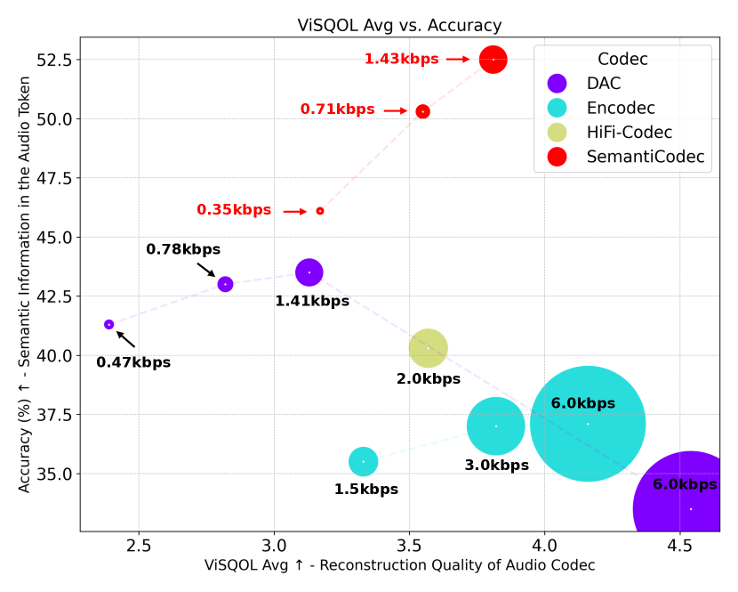
Figure 1: Comparison between SemantiCodec and state-of-the-art codecs. Larger values on the horizontal and vertical axis indicate better reconstruction quality and semantic information, respectively. The size of circles indicates bitrates, where smaller ones denote lower bitrates.

Despite the advancement in audio language modelling, the token rate of audio codecs has become a growing concern. For example, the token rate for a $6$ kbps Descript codec is $600$ per second. The auto-regressive (AR) nature of token generation means that the inference time of an audio language model scales with the length of codec tokens, posing challenges not only in computational efficiency but also in model training, where longer sequences demand more computational resources. Additionally, longer sequences may lead to challenges on long-term dependencies. Studies on long-context language models [18] indicate that language models do not effectively leverage long-term context, often superficially utilising it. While low-bitrate audio codecs are available, like the $1.5$ kbps version Encodec [6], their reconstruction quality, with strong artefacts introduced, often falls short of production standards. This situation underscores a crucial trade-off between efficiency and quality in audio codec development, highlighting the need for codecs that can achieve high-quality audio reconstruction at low bitrates.

The presence and richness of semantic information within token sequences play a crucial role in the learning of language models [19, 20]. Support for this assertion also comes from findings by Toraman et al. [10], who demonstrated that on six text processing tasks tokenizers operating at a higher level of granularity, such as byte pair encoding [21], could substantially outperform character-level tokenizers, which often require the model to expand more capacity for understanding. Despite these insights on the importance of semantic information in the tokens, our initial investigations reveal that existing audio codecs, already employed in audio language modelling, fall short of capturing adequate semantic information, even at relatively high bitrate settings. For instance, when employing the latent encodings of the $6.0$ kbps Descript codec [7] for classification tasks across seven benchmarks in the HEAR benchmark [22], the average accuracy is only $33\%$, as demonstrated in Section V-B. In contrast, without fine-tuning, a self-supervised pretrained AudioMAE encoder [23] results in a significantly higher accuracy of $65\%$. The classification accuracy is the indicator of semantic richness within codecs, which is crucial for audio language modelling. Moreover, our analysis indicates that using just the first vector quantization layer of the $6.0$ kbps Descript codec, which is often considered to be the most important layer and selected for audio language modelling [15], the classification accuracy drops even further to an average of $24\%$. This deficiency in capturing and encoding rich semantic information in audio codecs can potentially hinder the performance of audio language models.

In this paper, we introduce SemantiCodec, a novel audio codec designed to tackle the issues of excessive token rate and insufficient semantic encoding in current audio codecs. SemantiCodec exhibits richer semantic information and similar reconstruction quality with lower bitrates than previous codecs, as illustrated in Figure 1. Our approach uses the strong generative capabilities of diffusion models alongside the rich audio representations learned by the self-supervised AudioMAE. SemantiCodec processes mel-spectrograms through two encoders sequentially with two distinct vector quantization (VQ) layers. The first VQ layer is constructed using centroids derived from k-means clustering [24] performed on a large dataset of AudioMAE features, ensuring the capture of semantic information. In contrast, the second layer employs a conventional learnable VQ mechanism, enhancing the audio reconstruction fidelity of SemantiCodec. Our empirical analysis reveals that the semantic content is predominantly encoded within the first VQ layer, contributing over $95\%$ to the classification accuracy. However, integrating the second VQ layer is critical in significantly elevating the quality and intelligibility of audio reconstruction. The concatenated quantized outputs from both VQ layers serve as the conditional input for a latent diffusion model (LDM), which follows the architecture of AudioLDM [25]. The latent diffusion model utilizes the provided conditions to reconstruct high-quality audio after quantization. Our experiment shows SemantiCodec outperforms the state-of-the-art audio codec at a similar bitrate on reconstruction quality and contains significantly better semantic information on audio tokens, leading to improved classification accuracy in audio understanding. In summary, our contributions are listed as follows:

• We propose SemantiCodec, which leverages strong generative models and the rich feature learnt by self-supervised model for semantic-driven audio encoding and reconstruction.

• SemantiCodec achieves strong reconstruction performance across general audio types at exceptionally low token rates of $25$, $50$, and $100$ per second, surpassing counterparts operating at significantly higher token rates.

• Evaluation on audio classification benchmarks demonstrates the significantly richer semantic information in the token of SemantiCodec, even with a single layer of vector quantization, indicating strong potential in future audio language modelling with the SemantiCodec.

II Related Work

II-A Neural Audio Codecs

Traditional audio codecs, as detailed by Valin et al. [26] and Dietz et al. [27], have demonstrated their ability to achieve low latency audio compression across a variety of audio types. However, these traditional approaches often fail to deliver high-quality audio reconstruction at low-bitrate settings, such as $3.0$ kbps. Pioneering deep-learning-based audio codecs, Garbacea et al. [28] introduce the use of vector-quantized variational auto-encoders (VQ-VAEs) for learning neural codecs tailored to speech data. SoundStream [4] proposes a universal codec adaptable to various audio types, incorporating a residual vector quantization (RVQ) module to enhance the quantization process and a generative adversarial network (GAN) [29] to improve the reconstruction quality. Following a similar trajectory, Encodec [6] advances the capabilities of SoundStream by integrating multi-scale discriminators and a loss-balancing strategy for reconstruction training alongside an additional language model to facilitate further compression. HiFi-Codec [8] introduced group-residual vector quantization (GRVQ), a novel approach aimed at reducing the number of codebooks required while preserving the reconstruction quality. Descript codec [7] offers enhancements to Encodec, achieving significantly superior reconstruction performance.

To compare our proposed SemantiCodec with previous systems, our experimental analysis primarily focuses on evaluating the richness of semantic information and the quality of audio reconstruction.

II-B Semantic Audio Representation Learning

Self-supervised learning (SSL) has exhibited strong performance in audio representation learning. SSL models can be categorized into two types based on their pre-training tasks: discriminative SSL and reconstructive SSL. Discriminative SSL models, exemplified by HuBERT [30], COLA [31], and BEATs [32], employ strategies such as contrastive learning to differentiate between positive and negative pairs, or masked language modelling (MLM) techniques to predict the quantized labels of masked segments, leveraging contextual information. Conversely, reconstructive SSL models, such as AudioMAE [23], take inspiration from MLM principles but pivot towards reconstructing the original audio content from masked segments. Given the reconstructive nature of AudioMAE pre-training, the AudioMAE features are potentially more balanced in acoustic and semantic information than those derived from only discriminative pre-training. In this work, we develop SemantiCodec with an AudioMAE encoder as one of the fundamental components.

II-C Conditional Audio Generation

The development of generative models [33, 34, 35] has significantly propelled the field of conditional audio generation. Speech generation technologies [36, 37, 38] have evolved to produce speech conditioned on transcriptions and specific styles, such as speaker identity, emotion, and prosody. The generative model has also enabled novel tasks such as binaural sound synthesis [39] and synthetic speech quality refinement [40]. Meanwhile, the generation of music and sound effects has been extended to be conditioned on textual descriptions [12, 25, 41] and visual cues [42, 43], demonstrating the versatility of generative architecture.

Diffusion models [44] stand out for their exceptional generative capabilities in producing diverse and high-quality samples. Diffusion models offer a more tractable training process than GANs, emerging as a preferred choice for many researchers. To address the computational demands associated with training and inference in high-dimensional spaces, latent diffusion models [45] have been introduced. LDMs operate on a lower-dimensional latent space derived from a VAE, significantly reducing computational complexity while maintaining the generative power of traditional diffusion models. This approach has been successfully applied in various conditional audio generation models, including AudioLDM [25], TANGO [46], AudioSR [47] and Make-An-Audio [48], illustrating the flexibility of the diffusion model.

III SemantiCodec

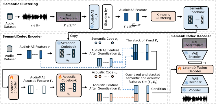
Figure 2: SemantiCodec architecture. For an input audio clip, quantized semantic representation ${\bm{E}}_{s}$ is obtained via a codebook pre-computed using k-means clustering on the AudioMAE embeddings. Then $\mathbf{Y}$ and $\mathbf{{\bm{E}}_{\text{s}}}$ are concatenated and fed to a residual encoder to complement acoustic details, which is discretized to ${\bm{E}}_{a}$ by a vector quantization module. SemantiCodec encoder output ${\bm{E}}$ is obtained by concatenating ${\bm{E}}_{s}$ and ${\bm{E}}_{a}$. A latent diffusion model is trained to generate the original audio clip conditioned on ${\bm{E}}$. The snowflake and fire symbols denote frozen and learnable parameters, respectively.

III-A System Overview

As shown in Figure 2, given an input audio ${\bm{x}}\in\mathbb{R}^{l}$, where $l$ denotes the sample length of audio, we initially transform ${\bm{x}}$ into the mel-spectrogram ${\bm{X}}\in\mathbb{R}^{T\times F}$, with $T$ and $F$ indicating the temporal and frequency dimensions, respectively. Leveraging a pretrained AudioMAE $\mathcal{A}(\cdot)$, we compute the AudioMAE feature $\tilde{{\bm{Y}}}=\mathcal{A}(X)=[\tilde{{\bm{y}}}_{1},\tilde{{\bm{y}}}_{2},\ldots,\tilde{{\bm{y}}}_{L}]\in\mathbb{R}^{L\times E}$, where $L=\frac{TF}{P^{2}}$ denotes the number of patch embedding vectors, and $P$ and $E$ represent the patch size and embedding size of AudioMAE, respectively. Each patch is a distinct, non-overlapping block of the mel-spectrogram processed by the AudioMAE, with multiple patches collectively forming the input to the AudioMAE encoder.

To reduce the number of patch embedding vectors, which directly influence the bitrate after quantization, we aggregate adjacent vectors of $\tilde{{\bm{Y}}}$ into ${\bm{Y}}=[{\bm{y}}_{1},{\bm{y}}_{2},\ldots,{\bm{y}}_{\frac{L}{K}}]\in\mathbb{R}^{\frac{L}{K}\times KE}$, where $K\in\{1,2,4\}$ is the stack factor, yielding ${\bm{y}}_{i}=[\tilde{{\bm{y}}}_{i},\ldots,\tilde{{\bm{y}}}_{i+K-1}]$ for $i\in\{1,2,\ldots,\frac{L}{K}\}$. Following extensive clustering on the vector ${\bm{y}}_{i}$, we derive the semantic codebook $\mathbb{E}_{\text{s}}=[{\bm{e}}_{1},{\bm{e}}_{2},\ldots,{\bm{e}}_{N_{\text{s}}}]$, where $N_{\text{s}}$ denotes the number of entries in the semantic codebook. We refer to this clustering process as semantic clustering.

The stacked feature ${\bm{Y}}$ undergoes initial quantization by $\mathbb{E}_{\text{s}}$ into semantic tokens ${\bm{c}}_{\text{s}}$ and semantic feature ${\bm{E}}_{\text{s}}\in\mathbb{R}^{\frac{L}{K}\times KE}$. Subsequently, we concatenate ${\bm{Y}}$ and ${\bm{E}}_{\text{s}}$, employing an acoustic encoder $\mathcal{F}(\cdot)$ to compute the acoustic feature ${\bm{Y}}_{\text{A}}$, which is then quantized via an acoustic vector quantization layer with entry $\mathbb{E}_{\text{a}}\in\mathbb{R}^{N_{\text{a}}\times E}$, outputting the acoustic tokens ${\bm{c}}_{\text{a}}$ and quantized acoustic feature ${\bm{E}}_{\text{a}}$. The final token for the input audio ${\bm{x}}$ is a merge of semantic and acoustic tokens: ${\bm{c}}=[{\bm{c}}_{\text{s}},{\bm{c}}_{\text{a}}]$.

The decoder of SemantiCodec utilizes a latent diffusion model conditioned on the concatenated quantized semantic and acoustic features ${\bm{E}}=[{\bm{E}}_{\text{s}},{\bm{E}}_{\text{a}}]$. The estimation of the latent diffusion model is further decoded back to waveform by a pretrained VAE decoder and a mel-spectrogram vocoder. The acoustic encoder $\mathcal{F}(\cdot)$ is joint-optimized with the acoustic codebook $\mathbb{E}_{\text{a}}$ and the latent diffusion model.

III-B Semantic Clustering

AudioMAE features stand out for their ability to preserve semantic and acoustic information [49], positioning them as highly effective features for reconstruction tasks. Additionally, AudioMAE features have demonstrated strong performance in downstream classification benchmarks [23]. Given these attributes, the AudioMAE feature is selected as the input for the SemantiCodec encoder, aiming to optimize audio reconstruction quality while ensuring the retention of semantic content.

We follow AudioLDM 2 [49] for AudioMAE feature extraction. Given an audio mel spectrogram representation ${\bm{X}}\in\mathbb{R}^{T\times F}$, the AudioMAE first transforms ${\bm{X}}$ into patches of dimensions $P\times P$. These patches form the inputs to the AudioMAE encoder, which leverages a design akin to the vision transformer [50]. The output ${\bm{Y}}_{0}$ of the AudioMAE encoder has a dimension of $\frac{T}{P}\times\frac{F}{P}\times E$, which can be viewed as a sequence of tensors with length $L=\frac{TF}{P^{2}}$ and an embedding dimension of $E$. We stack the adjacent $K$ frames of ${\bm{Y}}_{0}$ on the embedding dimension to form stacked AudioMAE feature vectors ${\bm{Y}}=\{{\bm{y}}_{1},{\bm{y}}_{2},\ldots,{\bm{y}}_{\frac{L}{K}}\}$, which are used both for semantic clustering and as the input of SemantiCodec encoder.

To perform semantic quantization on the AudioMAE feature vectors ${\bm{y}}_{i}$, we utilize k-means clustering [24], a widely used technique for partitioning a dataset into clusters in which each data point belongs to the cluster with the nearest mean. Our preliminary experiment indicates that the diverse acoustic characteristics of different audio types could lead to suboptimal outcomes when a single k-means clustering model is applied to a varied audio dataset. For instance, speech may necessitate finer granularity in clustering due to its rich semantic content, unlike more homogeneous sounds such as wind or church bells. We employ an ensemble clustering approach to overcome these issues and enhance semantic clustering accuracy, motivated by the cluster ensemble approach used in HuBERT [30]. This involves training distinct k-means models for three specific audio categories: speech, music, and general sounds. The codebooks derived from these domains are then merged, forming an ensembled codebook that accommodates the distinct acoustic features of each audio category, thereby optimising the clustering process for each unique audio type.

III-C SemantiCodec Encoder

As introduced in Section III-A, the encoding process of the SemantiCodec includes taking the stacked AudioMAE feature ${\bm{Y}}$ as input and calculating the token ${\bm{c}}=[{\bm{c}}_{\text{s}},{\bm{c}}_{\text{a}}]$ and the latent feature ${\bm{E}}=[{\bm{E}}_{\text{s}},{\bm{E}}_{\text{a}}]$. This part introduces the derivation of ${\bm{c}}$ and ${\bm{E}}$.

With the $N_{\text{s}}$ semantic codebook centroids ${\bm{e}}_{j}\in\mathbb{E}_{\text{s}}=\{{\bm{e}}_{1},{\bm{e}}_{2},\ldots,{\bm{e}}_{N_{\text{s}}}\}$, the semantic quantization process is given by

$$\small c_{\text{s}}(i)=\operatorname*{arg\,min}_{j\in\{1,\ldots,N_{\text{s}}\}}\|{\bm{y}}_{i}-{\bm{e}}_{j}\|^{2},{\bm{E}}_{\text{s}}(i)={\bm{e}}_{c_{\text{s}}(i)}\quad i\in\left\{1,2,\ldots,\frac{L}{K}\right\},$$ (1)

where $c_{\text{s}}(i)$ denotes the index of the closest centroid in the semantic codebook $\mathbb{E}_{\text{s}}$ to the feature vector ${\bm{y}}_{i}$, and ${\bm{E}}_{\text{s}}(i)$ is the centroid vector. This quantization step effectively maps each high-dimensional feature vector ${\bm{y}}_{i}$ into a discrete semantic token $c_{\text{s}}(i)$ and a corresponding quantized semantic feature ${\bm{E}}_{\text{s}}(i)$.

While the quantized AudioMAE feature ${\bm{E}}_{\text{s}}$ encapsulates rich semantic information, our experiments indicate that using ${\bm{E}}_{\text{s}}$ alone as the condition for audio reconstruction leads to sub-optimal quality (see Table I), such as unintelligible speech. To address this, we introduce an additional acoustic encoder module with vector quantization to capture discrete acoustic detail-oriented representations. The input feature we used for acoustic quantization is calculated by an acoustic encoder $\mathcal{F}_{\Phi}(\cdot)$, which takes the stack of the AudioMAE feature before and after semantic quantization as input and outputs the acoustic feature, given by

$${\bm{Y}}_{A}=\mathcal{F}_{\Phi}([{\bm{Y}},{\bm{E}}_{\text{s}}])\in\mathbb{R}^{\frac{L}{K}\times EK},$$ (2)

where $\Phi$ denotes the trainable parameter in the acoustic encoder. Specifically, we employ a bi-directional long short-term memory (BiLSTM) based network [51] as the acoustic encoder.

We use the quantization of ${\bm{Y}}_{A}$ to convert the detailed acoustic nuances into a compact, discrete format. We define the acoustic codebook as $\mathbb{E}_{\text{a}}=\{{\bm{e}}_{1},{\bm{e}}_{2},\ldots,{\bm{e}}_{N_{\text{a}}}\}$, where $N_{\text{a}}$ denotes the number of codebook entries and each ${\bm{e}}_{i}\in\mathbb{R}^{EK}$ represents an individual codebook vector. For each vector ${\bm{y}}_{a,i}\in{\bm{Y}}_{A}$, the quantization process is as follows:

$$\small c_{\text{a}}(i)=\operatorname*{arg\,min}_{j\in\{1,\ldots,N_{\text{a}}\}}\|{\bm{y}}_{a,i}-{\bm{e}}_{j}\|^{2},{\bm{E}}_{\text{a}}(i)={\bm{e}}_{c_{\text{a}}(i)}\quad i\in\{1,2,\ldots,\frac{L}{K}\},$$ (3)

where $c_{\text{a}}(i)$ identifies the index of the nearest centroid within the acoustic codebook $\mathbb{E}_{\text{a}}$ for the feature vector ${\bm{y}}_{a,i}$, and ${\bm{E}}_{\text{a}}(i)$ denotes the quantized vector. To encourage the acoustic encoder to produce representations that closely match the codebook entry and stabilise training, we employ a commitment loss [5], given by

$$\mathcal{L}_{\text{commit}}=\sum_{i}\|{\bm{y}}_{a,i}-{\bm{E}}_{\text{a}}(i)\|^{2}.$$ (4)

Following the success of HiFi-Codec [8], our approach utilizes an exponential moving average (EMA) mechanism for codebook update. The final tokens ${\bm{c}}$ and the representation ${\bm{E}}$ are the concatenation of output from both the semantic quantization layer and acoustic quantization layer, given by

$${\bm{c}}=[{\bm{c}}_{\text{s}},{\bm{c}}_{\text{a}}]\in\mathbb{N}^{\frac{2L}{K}},{\bm{E}}=[{\bm{E}}_{\text{s}},{\bm{E}}_{\text{a}}]\in\mathbb{R}^{\frac{L}{K}\times 2EK}.$$ (5)

Note that the dual-layer vector quantization architecture (semantic quantization and acoustic quantization) in SemantiCodec is different from residual vector quantization approach [4, 6], where the second layer aims to refine the codec encoder output directly. Instead, our approach allows the output of the second layer to be freely optimized in conjunction with the diffusion decoder for end-to-end training.

III-D Latent Diffusion Model for Reconstruction

Following the success of latent diffusion models (LDMs) for conditional audio generation [47, 25, 48], we employ an LDM as the decoder to reconstruct the original audio $x$. The LDM models the data distribution in a latent space constructed from a VAE, which is directly adopted from the VAE used in AudioLDM 2 [49]. Compared with the original diffusion model [52], the high-dimensional spectrogram ${\bm{X}}$ is compressed to the low-dimensional latent $\mathbf{z}_{0}$ in the LDM to significantly alleviate the computations. Then a diffusion model is trained to gradually generate $\mathbf{z}_{0}$ from the standard Gaussian noise. The forward diffusion process comprises a series of $N$ Markov transition steps that gradually transform $\mathbf{z}_{0}$ into a Gaussian distribution by noise injection. The forward step $n-1$ is defined as:

$$q(\mathbf{z}_{n}|\mathbf{z}_{n-1})=\sqrt{1-\beta_{n}}\mathbf{z}_{n-1}+\sqrt{\beta_{n}}\epsilon_{n},$$ (6)

where $\beta_{n}$ is the predefined noise schedule. By compositing these forward steps, we can derive the closed-form distribution of an arbitrary step $n$ given the initial $\mathbf{z}_{0}$ [52]:

$$q(\mathbf{z}_{n}|\mathbf{z}_{0})=\sqrt{\bar{\alpha}_{n}}\mathbf{z}_{0}+\sqrt{1-\bar{\alpha}_{n}}\epsilon_{n},$$ (7)

where $\alpha_{n}=1-\beta_{n},\bar{\alpha}_{n}=\prod_{n=1}^{n}\alpha_{n}$ and $\epsilon\sim\mathcal{N}(0,I)$. With enough diffusion steps $N$, $q(\mathbf{z}_{n})$ will approximate a standard Gaussian distribution $\mathcal{N}(0,I)$. The LDM is trained to model the reverse probability $p_{\theta}(\mathbf{z}_{n-1}|\mathbf{z}_{n},{\bm{E}})$ conditioned on the SemantiCodec encoder output ${\bm{E}}$.

Recent research by Lin et al. [53] has identified limitations in the prevalent noise scheduling techniques employed in diffusion models, specifically highlighting that the noisy latent at the last forward diffusion step $\mathbf{z}_{N}$ fails to follow a Gaussian distribution. To rectify this discrepancy, we adopt the strategy proposed by Lin et al.[53] and implement a cosine noise schedule. This modification guarantees the attainment of a standard Gaussian distribution in the last step of the diffusion process during training, thereby enhancing the consistency of the LDM between training and inference. To improve the generation performance and stabilize the sampling process, we switch the standard noise prediction objective to velocity prediction proposed in [54]. The LDM training loss [54] can be formulated as:

$${\bm{v}}_{n} =\sqrt{\bar{\alpha}_{n}}\epsilon-\sqrt{1-\bar{\alpha}_{n}}\mathbf{z}_{0},$$ (8)

$$\mathcal{L}_{\text{recon}} =\lVert{\bm{v}}_{n}-\mathcal{G}_{\theta}(\mathbf{z}_{n},n,{\bm{E}})\rVert^{2},$$ (9)

where $\mathcal{G}_{\theta}$ denotes the LDM and $\theta$ is the set of trainable parameters.

We adopt the DDIM sampler [55] for inference. Finally, the audio $\hat{{\bm{x}}}$ is reconstructed via the pretrained VAE decoder and a vocoder. The vocoder is a HiFi-GAN-based architecture [56] and is directly adopted from the pretrained AudioLDM 2. Our LDM adopts the Transformer-UNet (T-UNet) introduced in AudioLDM 2 [49], which incorporates self-attention and cross-attention Transformer blocks between convolutional blocks, significantly enhancing the model capacity to complex audio patterns. However, our experiments suggest that the impact of T-UNet parameter numbers, such as $75$ million or $346$ million, on the quality of audio reconstruction is relatively minor compared to their role in text-to-audio generation tasks. Therefore, we adopt a T-UNet with reduced parameter size compared with AudioLDM 2.

To achieve potentially better quality in reconstruction, we adopt classifier-free guidance [57, 58] (CFG), a common approach to guiding the audio generation by the diffusion models. The condition ${\bm{E}}$ in Equation 9 is randomly discarded with a certain probability during training so that both conditional generation models $v_{\theta}(\mathbf{z}_{n},n,{\bm{E}})$ and unconditional generation models $v_{\theta}(\mathbf{z}_{n},n)$ are optimized in a multi-task paradigm. During sampling, the original $v_{\theta}(\mathbf{z}_{n},n,{\bm{E}})$ is replaced by the weighted combination of velocities predicted by conditional and unconditional models:

$$(1-w)\cdot v_{\theta}(\mathbf{z}_{n},n,{\bm{E}})+w\cdot v_{\theta}(\mathbf{z}_{n},n),$$ (10)

where $w$ is the guidance scale. We show the effect of different CFG guidance scales in Figure 6.

III-E Training Objective

As shown in Figure 2, we keep the pretrained AudioMAE, VAE and vocoder parameters frozen. The k-means semantic clustering centroids are separately obtained before the training of the latent diffusion model and are also kept frozen. The acoustic encoder, acoustic vector quantization layer and the latent diffusion model are jointly optimized by a sum of the reconstruction loss and the commitment loss in the acoustic vector quantization layer, denoted by

$$\mathcal{L}=\mathcal{L}_{\text{recon}}+\mathcal{L}_{\text{commit}}.$$ (11)

IV Experimental Setup

IV-A Datasets

IV-A1 Training Datasets

Our model training is supported by various datasets, which can be generally classified into three categories: speech, music, and general sounds. For speech, we utilize the GigaSpeech (GGS) [59] dataset, a comprehensive English speech recognition corpus with around $10,000$ hours of transcribed audio, and the speech dataset collected by VoiceFixer [60] on OpenSLR, featuring a multi-lingual speech dataset with $186,514$ short audio clips. The music category includes the Million Song Dataset (MSD)[61], which provides a vast collection of $510,000$ music tracks with metadata. We also adopt datasets including MedleyDB [62], and MUSDB18 [63] training subset, mostly used for music source separation [64]. For general audio sounds, we engaged with AudioSet (AS)[65], the largest classification dataset offering two million ten-second audio clips across $527$ categories, WavCaps[66] that includes ChatGPT-assisted weakly-labeled audio captions for $403,050$ clips, and VGGSound (VS)[67], a substantial audio-visual dataset with around $190,000$ videos from which we only utilized the audio data. All the audio data are resampled to $16$kHz during training and evaluation. Our ablation studies in Section V-C2 and Section V-C3 utilize $10$% of the training data to speed up the model training.

IV-A2 Reconstruction Performance Evaluation

To assess the reconstruction capabilities of our audio codec, we carefully select and evaluate three distinct categories of datasets similar to building the training set. Within the speech category, we carefully choose a subset of the LibriTTS clean test set [68], selecting $300$ speech utterances randomly. These utterances, each lasting between $8$ and $10$ seconds, come with detailed transcription annotations, offering a rich basis for evaluating speech reconstruction accuracy. We randomly select $500$ segments from the AudioSet evaluation set for general audio evaluation, ensuring a diverse representation of ambient sounds, effects, and non-musical content. Our music data evaluation leverages the MUSDB18 test set [63], comprising $50$ songs with isolated tracks for vocals, drums, bass, and other elements. From each of the four tracks and their mixture for every song, we randomly select a $10$-second segment, ensuring it is non-silent, to form our evaluation set. Our evaluation dataset encompasses $1050$ audio samples, achieving a relatively balanced distribution across speech, music, and general sounds. Our MUSHRA (MUltiple Stimuli with Hidden Reference and Anchor) test is performed on the same evaluation dataset while only $10\%$ of the data is used to save effort for subjective evaluation. Our evaluation set and metrics implementations are publicly available.

IV-A3 Semantic Information Evaluation

To assess the richness of semantic information captured by audio codec representations, we employ a diverse array of datasets following a subset of the HEAR evaluation benchmark [22]. We choose the tasks oriented towards clip-level audio content classification, eliminating tasks like Gunshot Triangulation, which aims to recognize recording devices. Also, for convenience, we choose the datasets where the duration of each audio clip is shorter or close to $10$ seconds. The evaluation datasets we employed include the following: (i) NSynth Pitch (NSPitch) [69] is utilized to evaluate the ability to recognize musical pitches, a fundamental aspect of music theory and auditory perception. (ii) ESC-50 [70] encompasses a broad array of environmental sounds such as rainstorms and animal calls, testing the versatility of the codec feature towards general sound effects. (iii) LibriCount (LbCount) [71] is the dataset used to determine the number of speakers in an audio clip, combining speech detection with the differentiation of speakers within complex auditory scenes. (iv) CREMA-D (CRM-D) [72] focuses on speech emotion recognition, requiring models to classify a wide spectrum of emotional states conveyed through speech. (v) Vocal Imitations (VoImit) [73] dataset examines the ability to classify non-verbal human vocal imitations of various sounds. (vi) Speech Commands (SC) [74] dataset tests the recognition of specific spoken commands, emphasizing speech clarity and command accuracy. These audio classification datasets collectively offer a comprehensive evaluation framework, spanning musical notes, environmental sounds, speech nuances, and non-verbal vocalizations, to thoroughly assess the semantic capabilities of audio codec representations.

IV-B Baselines

We employ several state-of-the-art neural audio codecs as baselines for comparison, including Encodec (EC), Descript Codec (DAC), and HiFi-Codec (HC), which have demonstrated success in the domain of general sound. The open-sourced Encodec is trained on a variety of $24$kHz sampling rate audio data and can compress audio to $1.5$, $3.0$, $6.0$, $12.0$, and $24.0$ kbps. Since SemantiCodec operates at a relatively low bitrate, we only compare Encodec with $1.5$, $3.0$, and $6.0$ kbps settings. For DAC, we adopt the open-sourced $6.0$kbps model that operates on $16$kHz as one of the baselines. Since DAC does not have checkpoint open-sourced for a lower bitrate, we train another three variants of the DAC with the same training data as SemantiCodec following the setting described in their paper [7]. The three DAC settings have a bit rate of $0.47$, $0.78$, and $1.41$ kbps, which are comparable to the three variants of SemantiCodec. For HiFi-Codec, we adopt the $2.0$ kbps checkpoint.

IV-C Evaluation Metrics

IV-C1 Reconstruction Performance Evaluation

To assess the reconstruction quality of audio codecs with objective metrics, we employ mel spectrogram distance (MEL), short-time Fourier transform distance (STFT), and the virtual speech quality objective listener score (ViSQOL) [75]. MEL and STFT metrics quantify spectrogram discrepancies, with STFT providing a more nuanced capture of high-frequency fidelity. Our implementation for MEL and STFT follows the approach detailed in DAC [7], employing multiple window lengths to accommodate various audio signal types effectively. ViSQOL, a full-reference and intrusive perceptual quality metric, is designed to estimate the subjective mean opinion score (MOS) of audio quality. ViSQOL offers two modes for evaluation: an audio mode for 48kHz samples and a speech mode for 16kHz samples. Considering our focus on 16kHz audio codecs, we resample both the ground truth and reconstructed audio to 48kHz to leverage the audio mode for evaluations on the AudioSet and MUSDB18 datasets. Additionally, to evaluate the intelligibility of speech signals, we employ the word error rate (WER), a critical metric for evaluating the performance of automatic speech recognition systems by calculating the percentage of errors in the form of substitutions, deletions, or insertions relative to a reference transcript. We utilize the whisper-large-v3 [76] model to transcribe our reconstruction and remove all punctuations in the original LibriTTS transcriptions before calculating WER.

IV-C2 Semantic Information Evaluation

We assess the semantic distinctiveness of the audio codec representation by analyzing classification accuracy on the datasets described in Section IV-A, following the methodology outlined in the HEAR evaluation benchmark [22]. Our evaluation specifically focuses on the quantized output of the codec encoder, which serves as input to the codec decoder. The codec model is frozen to extract the quantized feature without fine-tuning. The feature sequence is averaged along the time axis to obtain the clip-level feature. A shallow downstream multi-layer perceptron (MLP) classifier with two linear layers is trained on clip-level features. The classification performance is reported to indicate the semantic distinctiveness of the codec. Furthermore, several studies on audio language models use powerful AR language models to predict tokens from the first VQ layer while leaving the rest tokens to be predicted by non-AR language models [15]. Therefore, we also report the classification performance using tokens from the first VQ layer to assess the semantic richness.

IV-C3 MUSHRA Test

To assess the subjective audio reconstruction quality of various audio codecs, we adhere to the established MUSHRA test protocol [77]. This method requires participants to evaluate audio samples relative to a concealed reference and predefined anchors, ensuring evaluators are unaware of the original clip to foster impartial assessments. Ratings are assigned on a scale from $0$ to $100$. For our MUSHRA evaluation, we randomly select $10$% of the audio from our evaluation set, comprising $25$ music tracks, $30$ speech recordings, and $50$ general sound samples. Participants are tasked with rating the audio quality of nine different samples, which include three variations each of SemanticCodec and Descript codecs at different bitrates, an open-source Encodec at $1.5$kbps, the original audio (ground truth), and an anchor with a low-pass filter applied at $3.5$ kHz. We ensure each set of audio receives evaluations from at least $10$ raters. Participants are instructed with This task evaluates the quality proximity between an audio sample and its reference. Please listen carefully to the reference audio and then rate the quality of each test audio clip compared to the reference. Use the scale where $0$ indicates no resemblance to the reference, and $100$ means perfectly the same as the reference. Ratings with ground truth scored below $60$ are excluded to maintain data integrity. Including deliberately degraded anchors allows the MUSHRA test to reveal subtle perceptual distinctions and quality variances across codecs. Our MUSHRA test has received a favourable opinion from the ethics review through completing the University of Surrey self-assessment governance and ethics form. We calculate and report the mean MUSHRA score for each codec as its final subjective evaluation metric.

IV-D Implementation Details

We implemented the k-means clustering on the high-dimensional AudioMAE features extracted from our dataset, as mentioned in Section IV-A. This procedure was carried out individually for three types of audio: music, speech, and general sound. For each type of audio, we run the clustering with different numbers of centroids, including $1024$, $2048$, $4096$, $8192$, and $16384$, to produce $15$ distinct sets of centroids. To manage the computational complexity of clustering high-dimensional features, we made several optimizations to the algorithm, which is available online.

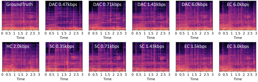
Figure 3: The log-STFT spectrogram of the ground truth audio and the reconstruction audio with different audio codecs. DAC, EC, HC, and SC are the descript codec, Encodec, HiFi-Codec, and SemantiCodec, respectively.

In building the final semantic codebook for SemantiCodec, we combined codebooks from each of the three audio domains. Given that general audio tends to encompass a broader array of sounds than speech and music, we assigned twice as many centroids. This created four distinct semantic codebooks with varying centroids: $4096$, $8192$, $16384$, and $32768$. For example, the codebook with $16384$ centroids includes $8192$ centroids for general audio and $4096$ centroids each for speech and music. This selection and combination process ensures our SemantiCodec has a comprehensive semantic codebook that accurately captures the diverse range of audio it processes. We repeat the above clustering and merging process for three different settings of stack factors $K\in\{1,2,3\}$. We randomly select and employ one of the four semantic codebooks in each training batch during model optimization. Therefore, our model supports variable vocabulary sizes and bitrates. The acoustic codebook utilizes a fixed-size codebook. We employ $32768$ centroid semantic codebook and $8192$ centroid acoustic codebook by default during model evaluation. Our experiment result indicates that more semantic centroids can moderately improve the reconstruction quality (see Figure 5).

We utilize the AudioMAE model pretrained on AudioSet, which features an embedding dimension of $768$. The resulting feature dimension is $K\times 768$ when stacking adjacent frames. Our implementation strategy for both the AudioMAE encoder and the diffusion decoder aligns with the approach described in AudioLDM 2. A notable modification in our setup is the adoption of a more compact T-UNet architecture with a base channel number of $64$ and a parameter number of $75$ million, in contrast to the larger version in AudioLDM 2 which features a base channel number of $128$ with $346$-million parameters. SemantiCodec is configured to operate at three different token rate settings, including $25$, $50$, and $100$ tokens per second. For each setting, the model undergoes training for $500,000$ steps on the designated training set with two A100-Amphere-$80$GB GPUs with a batch size of $48$. With a basic learning rate of $1e-4$, we incorporate a linear warm-up phase over the first $5,000$ steps. In the T-UNet architecture, the output from the SemantiCodec encoder, denoted as ${\bm{E}}$, is integrated via cross-attention mechanisms. Given that ${\bm{E}}$ lacks inherent positional information, we enrich it with fixed positional embeddings before input into the cross-attention layers.

SemantiCodec is trained on audio segments exactly $10.24$ seconds in length. To accommodate audio files of varying lengths, we have developed solutions involving either trimming or an overlap-and-add approach. For audio files shorter than $10.24$ seconds, we pad them to the required duration, compute the token encoding, and then remove any tokens corresponding to the padded region. For files longer than $10.24$ seconds, we segment the audio into $10.24$-second chunks without overlap, compute their token embeddings, and concatenate these segments. During inference, decoding uses a window length of $10.24$ seconds with a $6.25\%$ overlap between consecutive windows. The audio content from overlapping segments is blended using a linear decay and gain before combining.

V Results

V-A Reconstruction Quality

TABLE I: Objective evaluation of SemantiCodecs and competing baseline codecs at various bitrates on speech, music and general audio. VIS stands for the ViSQOL metric.

			General Audio			Music			Speech				Average
Model	kBit/Sec	Token/Sec	MEL$\downarrow$	STFT$\downarrow$	VIS$\uparrow$	MEL$\downarrow$	STFT$\downarrow$	VIS$\uparrow$	MEL$\downarrow$	STFT$\downarrow$	VIS$\uparrow$	WER$\downarrow$	VIS$\uparrow$
GroudTruth	$-$	-	$0.0$	$0.0$	$4.99$	$0.0$	$0.0$	$4.99$	$0.0$	$0.0$	$4.99$	$2.09$	$4.99$
SemantiCodec w. GT AudioMAE	$-$	-	$3.78$	$3.89$	$4.58$	$3.79$	$3.40$	$4.56$	$3.77$	$3.18$	$4.71$	$2.7$	$4.61$
SemantiCodec w.o. Acoustic VQ	$0.71$	$50$	$7.29$	$4.93$	$2.43$	$7.67$	$4.44$	$2.61$	$8.68$	$4.58$	$2.78$	$55.6$	$2.61$
DAC	$6.00$	$600$	$2.91$	$3.03$	$4.36$	$2.83$	$2.90$	$4.54$	$2.79$	$2.92$	$4.71$	$3.0$	$4.54$
	$6.00$	$600$	$4.38$	$4.10$	$4.00$	$4.17$	$2.90$	$4.14$	$4.54$	$3.19$	$4.35$	$3.3$	$4.16$
	$3.00$	$300$	$4.84$	$4.26$	$3.58$	$4.67$	$3.11$	$3.78$	$5.06$	$3.40$	$4.10$	$3.7$	$3.82$
Encodec	$1.50$	$150$	$5.39$	$4.47$	$3.04$	$5.30$	$3.33$	$3.27$	$5.83$	$3.67$	$3.67$	$5.0$	$3.33$
HiFi-Codec	$2.00$	$200$	$4.35$	$3.61$	$3.11$	$4.37$	$3.11$	$3.42$	$3.93$	$2.99$	$4.18$	$3.6$	$3.57$
	$0.47$	$47$	$7.56$	$4.58$	$2.12$	$7.80$	$4.24$	$2.33$	$8.62$	$4.70$	$2.73$	$28.2$	$2.39$
	$0.78$	$78$	$6.73$	$4.41$	$2.47$	$6.44$	$3.88$	$2.80$	$6.76$	$4.13$	$3.19$	$11.6$	$2.82$
DAC	$1.41$	$141$	$6.56$	$4.78$	$2.85$	$6.30$	$3.72$	$3.10$	$6.71$	$3.91$	$3.44$	$5.0$	$3.13$
	$0.36$	$25$	$5.06$	$4.02$	$2.84$	$5.22$	$3.76$	$3.18$	$5.77$	$3.72$	$3.49$	$19.6$	$3.17$
	$0.71$	$50$	$4.67$	$3.97$	$3.20$	$4.74$	$3.62$	$3.54$	$4.95$	$3.49$	$3.92$	$5.1$	$3.55$
SemantiCodec	$1.43$	$100$	$4.39$	$3.79$	$3.48$	$4.44$	$3.56$	$3.80$	$4.54$	$3.38$	$4.17$	$3.4$	$3.81$

Table I shows the audio reconstruction quality of SemantiCodec and baselines described in Section IV-B indicated by objective metrics. We use Token/Sec to denote the number of tokens the audio signal is encoded into per second, which is crucial in audio language modelling as it influences the length of the audio sequence. Given the variability in semantic codebook sizes, models with identical Token/Sec may yield different bit rates (see Figure 5), denoted by kBit/Sec or Kbps. SemantiCodec significantly outperforms the reconstruction quality compared with DAC at similar bitrates. With a low bitrate of $0.71$kbps, the reconstruction quality of SemantiCodec still outperforms the $1.5$kbps Encodec. It is remarkably comparable to HiFi-Codec operating at $2.0$kbps, as the average ViSQOL score indicates. With an ultra-low bitrate of $0.36$kbps, SemantiCodec still achieves a better ViSQOL score than the $1.41$kbps DAC. The $1.43$ kbps SemantiCodec demonstrate performance on par with the $3.0$ kbps Encodec. The superior performance of SemantiCodec in reconstruction at low bitrates indicates its potential in efficient audio transmission and storage and audio-based language modelling since it provides shorter discrete representations of audio without substantially compromising the reconstruction quality.

Using the ground truth unquantized AudioMAE feature as the condition for the latent diffusion model, the setting SemantiCodec w. GT AudioMAE marks the performance upper bound of SemantiCodec. SemantiCodec w. GT AudioMAE demonstrates strong performance on the reconstruction quality with an average ViSQOL score of $4.61$, which indicates that the original AudioMAE feature contains sufficient information to reconstruct the audio signal. However, the metrics MEL and STFT are still considerably lower than other neural codecs, which is expected because SemantiCodec does not directly employ MEL and STFT as the training objective.

By removing the second VQ layer, as shown in the setting of SemantiCodec w.o. Acoustic VQ, the model performance exhibit a considerable degradation, with a WER of $55.6$ and a ViSQOL of $2.61$, highlighting the importance of the second acoustic VQ layer for acoustic reconstruction. Finally, comparing the reconstruction performance across different audio types, it can be concluded that general audio consistently exhibits a slightly inferior reconstruction quality than music and speech. The challenges in reconstructing general audio signals may be attributed to the intrinsic complexity and variability of general audio content. This also validates our choice of assigning more semantic centroid numbers for general audio than speech and music in Section IV-D.

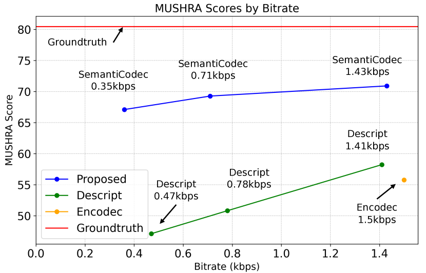
Figure 4: The average MUSHRA test score on our curated evaluation set. Our proposed SemantiCodec outperforms the baseline model even with a significantly lower bitrate.

Figure 4 further showcases the reconstruction performance in terms of subjective MUSHRA scores. We only incorporate codecs with a bitrate of less than or equal to $1.5$kbps into evaluation since we aim at developing codecs with ultra-low bitrates. The result is consistent with the objective evaluation shown in Table I that SemantiCodec significantly outperforms counterparts with a similar or even higher bitrate. With the reference audio being scored to $80.4$, the $1.5$kbps Encodec model achieves a $55.7$ average MUSHRA score, while even our $0.35$ kbps SemantiCodec achieves a significantly higher score of $67.1$. The high MUSHRA score of SemantiCodec can be attributed to the generative nature of the model, which leads to better audio quality at ultra-low bitrate. By comparison, we observe strong artifacts at similar bitrates on DAC and Encodec (shown in Figure 3), which can significantly impact the listener quality.

V-B Semantic in the Codec Tokens

TABLE II: Semantic evaluation of SemantiCodecs and competing baseline codecs using the HEAR benchmark.

VQ setting	Model	kBit/Sec	Token/Sec	ESC-50	NSPitch	SPC	LbCount	CRM-D	VoImit	Average ACC
Unquantized	AudioMAE	-	-	$79.5$	$82.0$	$48.0$	$69.4$	$67.3$	$17.4$	$60.6$
All VQ layers	Encodec	$6.00$	$600$	$40.7$	$60.8$	$27.3$	$45.0$	$44.2$	$4.4$	$37.1$
	HiFi-Codec	$2.00$	$200$	$36.3$	$71.0$	$26.5$	$58.2$	$45.6$	$4.3$	$40.3$
	DAC	$6.00$	$600$	$33.4$	$56.1$	$21.0$	$46.4$	$39.9$	$3.4$	$33.4$
		$1.41$	$141$	$41.1$	$\mathbf{80.9}$	$30.3$	$59.5$	$44.7$	$4.8$	$43.5$
		$0.78$	$78$	$39.5$	$78.5$	$30.3$	$59.5$	$45.7$	$5.0$	$43.0$
		$0.47$	$47$	$36.7$	$75.7$	$26.4$	$59.6$	$44.5$	$4.9$	$41.3$
	SemantiCodec	$1.43$	$100$	$\mathbf{63.8}$	$73.3$	$\mathbf{43.6}$	$67.0$	$\mathbf{57.9}$	$\mathbf{9.6}$	$\mathbf{52.5}$
		$0.71$	$50$	$60.9$	$64.9$	$41.9$	$\mathbf{71.6}$	$53.2$	$9.3$	$50.3$
		$0.35$	$25$	$56.4$	$61.3$	$33.7$	$70.4$	$46.9$	$8.0$	$46.1$
First VQ Layer	Encodec	$0.75$	$75$	$32.0$	$45.3$	$23.0$	$44.8$	$40.7$	$4.2$	$31.6$
	HiFi-Codec	$1.00$	$100$	$33.7$	$58.9$	$25.9$	$58.3$	$44.3$	$4.1$	$37.5$
	DAC ($6.00$k)	$0.5$	$50$	$23.8$	$23.3$	$15.9$	$43.1$	$38.4$	$3.1$	$24.6$
	DAC ($1.41$k)	$0.16$	$16$	$29.0$	$44.2$	$19.9$	$57.0$	$39.5$	$4.0$	$32.3$
	DAC ($0.78$k)	$0.16$	$16$	$27.6$	$39.9$	$17.9$	$56.6$	$40.9$	$4.0$	$31.1$
	DAC ($0.36$k)	$0.16$	$16$	$29.7$	$46.9$	$18.3$	$58.2$	$43.0$	$4.0$	$33.3$
	SemantiCodec	$0.71$	$50$	$\mathbf{66.6}$	$\mathbf{73.9}$	$\mathbf{42.7}$	$\mathbf{66.7}$	$\mathbf{57.5}$	$\mathbf{11.1}$	$\mathbf{53.1}$
		$0.36$	$25$	$64.4$	$70.2$	$36.0$	$65.0$	$54.1$	$10.7$	$50.1$
		$0.18$	$13$	$59.6$	$66.3$	$30.7$	$61.3$	$45.8$	$9.8$	$45.6$

The semantic richness of different codecs is demonstrated in Table II. First, when all VQ layers are utilized, SemantiCodec significantly outperforms baseline models in semantic information. Notably, even at a low bitrate of $0.35$kbps, the semantic performance of SemantiCodec surpasses that of higher bitrate counterparts like the $6.0$kbps Encodec and DAC. This indicates that AudioMAE features serve as effective means of semantic encoding.

Then, comparing codecs at different bitrates below $1.5$kbps, both DAC and SemantiCodec exhibit a decline in semantic performance as the bitrate decreases. However, even at the lowest bitrate of $0.35$kbps, SemantiCodec outperforms DAC at $1.41$kbps. Interestingly, despite the inferior reconstruction quality of DAC at lower bitrates, the semantic richness retained at low bitrates is significantly better than that of $6.0$kbps. This may be attributed to the information bottleneck imposed on the encoded representations during training with low bitrates. The model must preserve coarse audio contents in representations while discarding acoustic details, making the classifier easier to train on downstream tasks.

Since many studies utilize tokens from the first VQ layer to train audio language models, we investigate the semantic information in tokens under this situation. As shown in the lower part of Table II, baseline codecs exhibit a substantial drop in semantic performance when switching from full VQ layers to the first layer. For example, the first VQ layer of the $6.0$kbps DAC only achieves an average accuracy of $24.6$. In contrast, SemantiCodec maintains similar semantic accuracy with only the first VQ layer. This supports our assumption that semantic information is primarily encoded by semantic codes obtained through k-means clustering of AudioMAE features, with acoustic details augmented by subsequent acoustic codes. However, there is still a performance gap between unquantized AudioMAE features (ACC $60.6$) and the quantized latent space of SemantiCodec (ACC $53.1$), highlighting the need for further research into mitigating the loss caused by quantization.

V-C Ablation Study

TABLE III: Utilizing a variable semantic codebook size is beneficial for the reconstruction quality, compared with using a fixed semantic codebook with size $32768$.

	fixed vocab size		variable vocab size
Stack Factor	ViSQOL-Avg	WER	ViSQOL-Avg	WER
$K=1$	$3.78$	$3.6$	$3.81$	$3.4$
$K=2$	$3.41$	$6.3$	$3.55$	$5.1$
$K=4$	$3.04$	$21.8$	$3.17$	$19.6$

V-C1 Variable Semantic Codebook Size

As detailed in Section IV-D, during training, we employ a variety of semantic codebooks, enabling SemantiCodec to accommodate different vocabulary sizes. To explore the efficacy of this approach, we conduct experiments comparing a fixed vocabulary size against a variable one, maintaining a semantic codebook size of $32,768$ in both scenarios. We investigate different stack factors $K$ to assess their impact on performance. As presented in Table III, utilizing a variable vocabulary size significantly enhances the average ViSQOL score and reduces the WER. This improvement likely stems from the exposure to diverse codebooks during training, which enhances the ability of the model to interpret and process the quantized AudioMAE features effectively.

TABLE IV: The impact of k-means centroid number on the semantic richness of SemantiCodec.

K-means Centroids	ACC
$4096$	$49.0$
$8192$	$50.9$
$16384$	$52.1$
$32768$	$\mathbf{53.1}$

We also study the effect of semantic codebook size on semantic richness by calculating classification accuracy with the quantized AudioMAE feature. Table IV shows as the centroid number increases, the quantization error induced by k-means modelling is reduced, hence the semantic performance consistently improves. Similar behaviour can be observed in the reconstruction performance, as shown in Figure 5. With more k-means centroids (i.e., semantic vocabulary size) used, reconstructed speech quality steadily improves. However, as shown by Figure 5, higher semantic vocab size can impact the bitrate, posing a trade-off between reconstruction quality and bitrate.

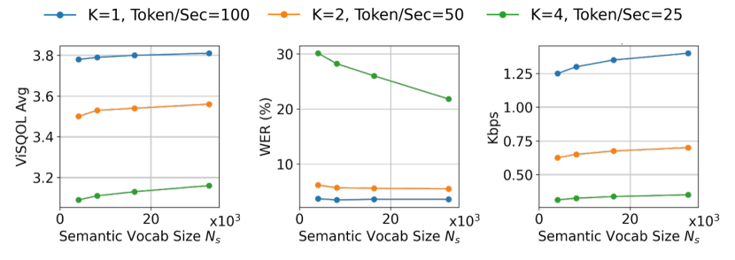
Figure 5: The impact of semantic vocabulary size on average ViSQOL, WER, and bitrate.

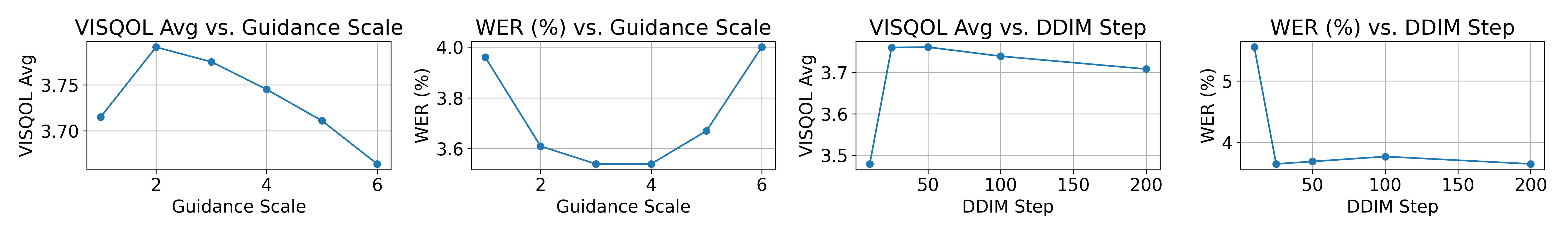
Figure 6: The impact of CFG guidance scale and DDIM sampling steps on reconstruction quality.

V-C2 Acoustic Representation Learning

The size of the acoustic codebook determines the granularity of the trainable vector quantization module. Analogous to the influence of k-means centroid numbers, larger codebook size leads to better reconstruction quality, as indicated by Table V.

The complexity of the LSTM acoustic encoder influences its capacity to refine and augment quantized AudioMAE features. Replacing the original bi-directional LSTM with a unidirectional one results in a significant drop in speech reconstruction quality, as indicated by WER. This validates the necessity of the bidirectional connection in the LSTM for efficiently extracting and encoding the contextual information and dependencies of AudioMAE feature sequences.

TABLE V: The impact of SemantiCodec encoder parameters on the reconstruction quality.

Acoustic Codebook Size	LSTM Bi-directional	VISQOL Avg	WER (%)
$8192$	✓	$\mathbf{3.602}$	$\mathbf{4.57}$
$4096$	✓	$3.583$	$5.05$
$2048$	✓	$3.550$	$4.66$
$8192$	✗	$3.596$	$4.80$

V-C3 Learnable Semantic Codebook

TABLE VI: The impact of replacing the k-means centroid with a learnable vector quantization layer.

SemantiCodec	ViSQOL   $\uparrow$	WER   $\downarrow$	ACC   $\uparrow$
Original	$\mathbf{3.60}$	$\mathbf{4.57}$	$\mathbf{53.1}$
Learnable Semantic VQ	$3.57$	$5.1$	$28.5$

The semantic codebook in SemantiCodec is frozen during model training. To validate the importance of performing k-means clustering beforehand, we conduct another experiment by replacing the semantic codebook with a learnable VQ layer, similar to the acoustic VQ layer. As shown in Table VI, even though the reconstruction performance of SemantiCodec is not largely affected without the use of k-means centroids, the semantic evaluation accuracy shows a notable decrease from $53.1$% to $28.5$%. This indicates the validity of k-means centroids used in the semantic codebook for maintaining rich semantic information in audio tokens. Directly training a codec model with two VQ layers results in the codec neglecting semantic information and focusing solely on reconstruction capabilities, as the training loss function is limited to reconstruction loss.

V-C4 DDIM Sampling Setups

As shown in Figure 6, the guidance scale $w$ (see Equation 10) in CFG can influence the reconstruction quality. CFG does not provide enough condition-oriented guidance through unconditional generation probability when the scale is too small. Conversely, when the scale is too large, the effect of the condition is diluted by the emphasis towards unconditional generation probability. Therefore, $w$ with values that are too small or too large leads to unsatisfactory reconstruction quality. The best reconstruction quality is achieved under a moderate scale near $3.0$.

The sampling step also plays a crucial role in the reconstruction quality of our latent diffusion decoder. The reconstruction quality of SemantiCodec is moderate, with a small number of sampling steps, e.g., ten steps. With a sampling step larger than $25$, the reconstruction quality significantly improves. This is promising for rapid sampling during audio reconstruction with tokens from SemantiCodec.

VI Conclusion

In this study, we have proposed SemantiCodec, an audio codec which can be applied to diverse audio types with ultra-low bitrates and rich semantic information in the audio tokens. SemantiCodec supports several bitrates between $0.31$kbps and $1.43$kbps. With a semantic and acoustic decoupled architecture, SemantiCodec achieves effective compression without significantly sacrificing quality with a token rate of $50$ per second and $100$ per second. At an ultra-low rate of $25$ tokens per second, SemantiCodec still demonstrates significantly strong audio quality compared with state-of-the-art audio codecs. Our experiment result also shows that the semantic information within the SemantiCodec tokens is significantly richer than previous neural audio codecs.

References

- [1] K. C. Pohlmann, Principles of digital audio. McGraw-Hill Professional, 2000.
- [2] J. Sterne, MP3: The meaning of a format. Duke University Press, 2012.
- [3] J. M. Valin, K. Vos, and T. B. Terriberry, “Definition of the opus audio codec,” Internet Engineering Task Force Standard, 2012.
- [4] N. Zeghidour, A. Luebs, A. Omran, J. Skoglund, and M. Tagliasacchi, “SoundStream: An end-to-end neural audio codec,” IEEE/ACM Transactions on Audio, Speech, and Language Processing, vol. 30, pp. 495–507, 2021.
- [5] A. Van Den Oord, O. Vinyals et al., “Neural discrete representation learning,” Advances in Neural Information Processing Systems, vol. 30, 2017.
- [6] A. Défossez, J. Copet, G. Synnaeve, and Y. Adi, “High fidelity neural audio compression,” Transactions on Machine Learning Research, 2023.
- [7] R. Kumar, P. Seetharaman, A. Luebs, I. Kumar, and K. Kumar, “High-fidelity audio compression with improved rvqgan,” Advances in Neural Information Processing Systems, vol. 36, 2024.
- [8] D. Yang, S. Liu, R. Huang, J. Tian, C. Weng, and Y. Zou, “HiFi-Codec: Group-residual vector quantization for high fidelity audio codec,” arXiv preprint:2305.02765, 2023.
- [9] Z. Borsos, R. Marinier, D. Vincent, E. Kharitonov, O. Pietquin, M. Sharifi, D. Roblek, O. Teboul, D. Grangier, M. Tagliasacchi et al., “AudioLM: A language modeling approach to audio generation,” IEEE/ACM Transactions on Audio, Speech, and Language Processing, vol. 42, pp. 2523–2544, 2023.
- [10] C. Toraman, E. H. Yilmaz, F. Şahinuç, and O. Ozcelik, “Impact of tokenization on language models: An analysis for turkish,” ACM Transactions on Asian and Low-Resource Language Information Processing, vol. 22, no. 4, pp. 1–21, 2023.
- [11] H. Touvron, T. Lavril, G. Izacard, X. Martinet, M.-A. Lachaux, T. Lacroix, B. Rozière, N. Goyal, E. Hambro, F. Azhar et al., “Llama: Open and efficient foundation language models,” arXiv preprint:2302.13971, 2023.
- [12] F. Kreuk, G. Synnaeve, A. Polyak, U. Singer, A. Défossez, J. Copet, D. Parikh, Y. Taigman, and Y. Adi, “AudioGen: Textually guided audio generation,” International Conference on Learning Representations, 2022.
- [13] A. Agostinelli, T. I. Denk, Z. Borsos, J. Engel, M. Verzetti, A. Caillon, Q. Huang, A. Jansen, A. Roberts, M. Tagliasacchi et al., “MusicLM: Generating music from text,” arXiv preprint:2301.11325, 2023.
- [14] J. Copet, F. Kreuk, I. Gat, T. Remez, D. Kant, G. Synnaeve, Y. Adi, and A. Défossez, “Simple and controllable music generation,” arXiv preprint:2306.05284, 2023.
- [15] C. Wang, S. Chen, Y. Wu, Z. Zhang, L. Zhou, S. Liu, Z. Chen, Y. Liu, H. Wang, J. Li et al., “Neural codec language models are zero-shot text to speech synthesizers,” arXiv preprint:2301.02111, 2023.
- [16] Y. Gong, H. Luo, A. H. Liu, L. Karlinsky, and J. R. Glass, “Listen, think, and understand,” in International Conference on Learning Representations, 2023.
- [17] P. K. Rubenstein, C. Asawaroengchai, D. D. Nguyen, A. Bapna, Z. Borsos, F. d. C. Quitry, P. Chen, D. E. Badawy, W. Han, E. Kharitonov et al., “AudioPaLM: A large language model that can speak and listen,” arXiv preprint:2306.12925, 2023.
- [18] S. Sun, K. Krishna, A. Mattarella-Micke, and M. Iyyer, “Do long-range language models actually use long-range context?” arXiv preprint:2109.09115, 2021.
- [19] T. Brychcín and M. Konopík, “Semantic spaces for improving language modeling,” Computer Speech & Language, vol. 28, no. 1, pp. 192–209, 2014.
- [20] A. O. Bayer and G. Riccardi, “Semantic language models with deep neural networks,” Computer Speech & Language, vol. 40, pp. 1–22, 2016.
- [21] Y. Shibata, T. Kida, S. Fukamachi, M. Takeda, A. Shinohara, T. Shinohara, and S. Arikawa, “Byte Pair Encoding: A text compression scheme that accelerates pattern matching,” 1999.
- [22] J. Turian, J. Shier, H. R. Khan, B. Raj, B. W. Schuller, C. J. Steinmetz, C. Malloy, G. Tzanetakis, G. Velarde, K. McNally et al., “HEAR: Holistic evaluation of audio representations,” in NeurIPS Competitions and Demonstrations Track, 2022, pp. 125–145.
- [23] P.-Y. Huang, H. Xu, J. Li, A. Baevski, M. Auli, W. Galuba, F. Metze, and C. Feichtenhofer, “Masked autoencoders that listen,” Advances in Neural Information Processing Systems, vol. 35, pp. 28 708–28 720, 2022.
- [24] J. MacQueen, “Some methods for classification and analysis of multivariate observations,” in Berkeley Symposium on Mathematical Statistics and Probability, vol. 1, no. 14, 1967, pp. 281–297.
- [25] H. Liu, Z. Chen, Y. Yuan, X. Mei, X. Liu, D. Mandic, W. Wang, and M. D. Plumbley, “AudioLDM: Text-to-audio generation with latent diffusion models,” International Conference on Machine Learning, 2023.
- [26] J.-M. Valin, K. Vos, and T. Terriberry, “Definition of the opus audio codec,” Tech. Rep., 2012.
- [27] M. Dietz, M. Multrus, V. Eksler, V. Malenovsky, E. Norvell, H. Pobloth, L. Miao, Z. Wang, L. Laaksonen, A. Vasilache et al., “Overview of the evs codec architecture,” in IEEE International Conference on Acoustics, Speech and Signal Processing. IEEE, 2015, pp. 5698–5702.
- [28] C. Gârbacea, A. van den Oord, Y. Li, F. S. Lim, A. Luebs, O. Vinyals, and T. C. Walters, “Low bit-rate speech coding with vq-vae and a wavenet decoder,” in IEEE International Conference on Acoustics, Speech and Signal Processing. IEEE, 2019, pp. 735–739.
- [29] A. Creswell, T. White, V. Dumoulin, K. Arulkumaran, B. Sengupta, and A. A. Bharath, “Generative adversarial networks: An overview,” IEEE Signal Processing Magazine, vol. 35, no. 1, pp. 53–65, 2018.
- [30] W.-N. Hsu, B. Bolte, Y.-H. H. Tsai, K. Lakhotia, R. Salakhutdinov, and A. Mohamed, “HuBERT: Self-supervised speech representation learning by masked prediction of hidden units,” IEEE/ACM Transactions on Audio, Speech, and Language Processing, vol. 29, pp. 3451–3460, 2021.
- [31] A. Saeed, D. Grangier, and N. Zeghidour, “Contrastive learning of general-purpose audio representations,” in IEEE International Conference on Acoustics, Speech and Signal Processing. IEEE, 2021, pp. 3875–3879.
- [32] S. Chen, Y. Wu, C. Wang, S. Liu, D. Tompkins, Z. Chen, W. Che, X. Yu, and F. Wei, “Beats: audio pre-training with acoustic tokenizers,” in Proceedings of International Conference on Machine Learning, 2023, pp. 5178–5193.
- [33] I. Goodfellow, J. Pouget-Abadie, M. Mirza, B. Xu, D. Warde-Farley, S. Ozair, A. Courville, and Y. Bengio, “Generative adversarial nets,” Advances in Neural Information Processing Systems, vol. 27, 2014.
- [34] D. P. Kingma and M. Welling, “Auto-encoding variational Bayes,” arXiv preprint:1312.6114, 2013.
- [35] D. Rezende and S. Mohamed, “Variational inference with normalizing flows,” in International conference on machine learning. Proceedings of Machine Learning Research, 2015, pp. 1530–1538.
- [36] V. Popov, I. Vovk, V. Gogoryan, T. Sadekova, and M. Kudinov, “Grad-TTS: A diffusion probabilistic model for text-to-speech,” in International Conference on Machine Learning, 2021, pp. 8599–8608.
- [37] J. Kim, J. Kong, and J. Son, “Conditional variational autoencoder with adversarial learning for end-to-end text-to-speech,” in Proceedings of International Conference on Machine Learning. PMLR, 2021, pp. 5530–5540.
- [38] X. Tan, J. Chen, H. Liu, J. Cong, C. Zhang, Y. Liu, X. Wang, Y. Leng, Y. Yi, L. He et al., “NaturalSpeech: End-to-end text to speech synthesis with human-level quality,” arXiv preprint:2205.04421, 2022.
- [39] Y. Leng, Z. Chen, J. Guo, H. Liu, J. Chen, X. Tan, D. Mandic, L. He, X.-Y. Li, T. Qin et al., “BinauralGrad: A two-stage conditional diffusion probabilistic model for binaural audio synthesis,” Advances in Neural Information Processing Systems, 2022.
- [40] Z. Chen, Y. Wu, Y. Leng, J. Chen, H. Liu, X. Tan, Y. Cui, K. Wang, L. He, S. Zhao, J. Bian, and D. Mandic, “ResGrad: Residual denoising diffusion probabilistic models for text to speech,” arXiv preprint:2212.14518, 2022.
- [41] K. Chen, Y. Wu, H. Liu, M. Nezhurina, T. Berg-Kirkpatrick, and S. Dubnov, “MusicLDM: Enhancing novelty in text-to-music generation using beat-synchronous mixup strategies,” in IEEE International Conference on Acoustics, Speech and Signal Processing. IEEE, 2024, pp. 1206–1210.
- [42] V. Iashin and E. Rahtu, “Taming visually guided sound generation,” in British Machine Vision Conference, 2021.
- [43] R. Sheffer and Y. Adi, “I hear your true colors: Image guided audio generation,” in IEEE International Conference on Acoustics, Speech and Signal Processing, 2023.
- [44] J. Ho, A. Jain, and P. Abbeel, “Denoising diffusion probabilistic models,” Advances in Neural Information Processing Systems, vol. 33, pp. 6840–6851, 2020.
- [45] R. Rombach, A. Blattmann, D. Lorenz, P. Esser, and B. Ommer, “High-resolution image synthesis with latent diffusion models,” in Proceedings of the IEEE/CVF Conference on Computer Vision and Pattern Recognition, 2022, pp. 10 684–10 695.
- [46] D. Ghosal, N. Majumder, A. Mehrish, and S. Poria, “Text-to-audio generation using instruction-tuned LLM and latent diffusion model,” arXiv preprint:2304.13731, 2023.
- [47] H. Liu, K. Chen, Q. Tian, W. Wang, and M. D. Plumbley, “Audiosr: Versatile audio super-resolution at scale,” in IEEE International Conference on Acoustics, Speech and Signal Processing, 2024, pp. 1076–1080.
- [48] R. Huang, J. Huang, D. Yang, Y. Ren, L. Liu, M. Li, Z. Ye, J. Liu, X. Yin, and Z. Zhao, “Make-An-Audio: Text-to-audio generation with prompt-enhanced diffusion models,” International Conference on Machine Learning, 2023.
- [49] H. Liu, Q. Tian, Y. Yuan, X. Liu, X. Mei, Q. Kong, Y. Wang, W. Wang, Y. Wang, and M. D. Plumbley, “Audioldm 2: Learning holistic audio generation with self-supervised pretraining,” arXiv preprint:2308.05734, 2023.
- [50] A. Dosovitskiy, L. Beyer, A. Kolesnikov, D. Weissenborn, X. Zhai, T. Unterthiner, M. Dehghani, M. Minderer, G. Heigold, S. Gelly et al., “An image is worth 16x16 words: Transformers for image recognition at scale,” in International Conference on Learning Representations, 2020.
- [51] H. Sak, A. Senior, and F. Beaufays, “Long short-term memory based recurrent neural network architectures for large vocabulary speech recognition,” arXiv preprint:1402.1128, 2014.
- [52] J. Ho, A. Jain, and P. Abbeel, “Denoising diffusion probabilistic models,” in Advances in Neural Information Processing Systems, H. Larochelle, M. Ranzato, R. Hadsell, M. Balcan, and H. Lin, Eds., vol. 33. Curran Associates, Inc., 2020, pp. 6840–6851.
- [53] S. Lin, B. Liu, J. Li, and X. Yang, “Common diffusion noise schedules and sample steps are flawed,” in Proceedings of the IEEE/CVF Winter Conference on Applications of Computer Vision, 2024, pp. 5404–5411.
- [54] T. Salimans and J. Ho, “Progressive distillation for fast sampling of diffusion models,” in International Conference on Learning Representations, 2021.
- [55] J. Song, C. Meng, and S. Ermon, “Denoising diffusion implicit models,” in International Conference on Learning Representations, 2020.
- [56] J. Kong, J. Kim, and J. Bae, “HiFi-GAN: Generative adversarial networks for efficient and high fidelity speech synthesis,” Advances in Neural Information Processing Systems, vol. 33, pp. 17 022–17 033, 2020.
- [57] J. Ho and T. Salimans, “Classifier-free diffusion guidance,” in NeurIPS Workshop on Deep Generative Models and Downstream Applications, 2021.
- [58] A. Q. Nichol, P. Dhariwal, A. Ramesh, P. Shyam, P. Mishkin, B. Mcgrew, I. Sutskever, and M. Chen, “GLIDE: Towards photorealistic image generation and editing with text-guided diffusion models,” in International Conference on Machine Learning, 2022, pp. 16 784–16 804.
- [59] G. Chen, S. Chai, G. Wang, J. Du, W. Q. Zhang, C. Weng, D. Su, D. Povey, J. Trmal, J. Zhang et al., “GigaSpeech: An evolving, multi-domain asr corpus with 10,000 hours of transcribed audio,” in INTERSPEECH, 2021, pp. 4376–4380.
- [60] H. Liu, Q. Kong, Q. Tian, Y. Zhao, D. Wang, C. Huang, and Y. Wang, “VoiceFixer: Toward general speech restoration with neural vocoder,” arXiv preprint:2109.13731, 2021.
- [61] T. Bertin-Mahieux, D. P. Ellis, B. Whitman, and P. Lamere, “The million song dataset,” International Society for Music Information Retrieval Conference, pp. 591–596, 2011.
- [62] R. M. Bittner, J. Salamon, M. Tierney, M. Mauch, C. Cannam, and J. P. Bello, “Medleydb: A multitrack dataset for annotation-intensive mir research.” in ISMIR, vol. 14, 2014, pp. 155–160.
- [63] Z. Rafii, A. Liutkus, F.-R. Stöter, S. I. Mimilakis, and R. Bittner, “The MUSDB18 corpus for music separation,” Dec. 2017. [Online]. Available: https://doi.org/10.5281/zenodo.1117372
- [64] Q. Kong, Y. Cao, H. Liu, K. Choi, and Y. Wang, “Decoupling magnitude and phase estimation with deep ResUNet for music source separation,” International Society for Music Information Retrieval Conference, pp. 342–349, 2021.
- [65] J. F. Gemmeke, D. P. Ellis, D. Freedman, A. Jansen, W. Lawrence, R. C. Moore, M. Plakal, and M. Ritter, “AudioSet: An ontology and human-labeled dataset for audio events,” in IEEE International Conference on Acoustics, Speech and Signal Processing, 2017, pp. 776–780.
- [66] X. Mei, C. Meng, H. Liu, Q. Kong, T. Ko, C. Zhao, M. D. Plumbley, Y. Zou, and W. Wang, “WavCaps: A ChatGPT-assisted weakly-labelled audio captioning dataset for audio-language multimodal research,” arXiv preprint:2303.17395, 2023.
- [67] H. Chen, W. Xie, A. Vedaldi, and A. Zisserman, “VGGSound: A large-scale audio-visual dataset,” in IEEE International Conference on Acoustics, Speech and Signal Processing, 2020, pp. 721–725.
- [68] H. Zen, V. Dang, R. Clark, Y. Zhang, R. J. Weiss, Y. Jia, Z. Chen, and Y. Wu, “Libritts: A corpus derived from librispeech for text-to-speech,” arXiv preprint:1904.02882, 2019.
- [69] J. Engel, C. Resnick, A. Roberts, S. Dieleman, M. Norouzi, D. Eck, and K. Simonyan, “Neural audio synthesis of musical notes with wavenet autoencoders,” in Proceedings of International Conference on Machine Learning, 2017, pp. 1068–1077.
- [70] K. J. Piczak, “ESC: Dataset for environmental sound classification,” in Proceedings of the ACM International Conference on Multimedia, 2015, pp. 1015–1018.
- [71] F.-R. Stöter, S. Chakrabarty, E. Habets, and B. Edler, “LibriCount: A dataset for speaker count estimation,” Apr 2018.
- [72] H. Cao, D. G. Cooper, M. K. Keutmann, R. C. Gur, A. Nenkova, and R. Verma, “Crema-d: Crowd-sourced emotional multimodal actors dataset,” IEEE Transactions on Affective Computing, vol. 5, no. 4, pp. 377–390, 2014.
- [73] B. Kim, M. Ghei, B. Pardo, and Z. Duan, “Vocal Imitation Set: a dataset of vocally imitated sound events using the audioset ontology.” in Workshop on Detection and Classification of Acoustic Scenes and Events, 2018, pp. 148–152.
- [74] P. Warden, “Speech Commands: A dataset for limited-vocabulary speech recognition,” arXiv preprint:1804.03209, 2018.
- [75] A. Hines, J. Skoglund, A. C. Kokaram, and N. Harte, “ViSQOL: an objective speech quality model,” EURASIP Journal on Audio, Speech, and Music Processing, vol. 2015, pp. 1–18, 2015.
- [76] A. Radford, J. W. Kim, T. Xu, G. Brockman, C. McLeavey, and I. Sutskever, “Robust speech recognition via large-scale weak supervision,” in Proceedings of International Conference on Machine Learning, 2023, pp. 28 492–28 518.
- [77] N. Schinkel-Bielefeld, N. Lotze, and F. Nagel, “Audio quality evaluation by experienced and inexperienced listeners,” in Proceedings of Meetings on Acoustics, vol. 19, no. 1, 2013.