Prescribed-Time Stability Properties of Interconnected Systems

Abstract

Achieving control objectives (e.g., stabilization or convergence of tracking error to zero, input-to-state stabilization) in “prescribed time” has attracted significant research interest in recent years. The key property of prescribed-time results unlike traditional “asymptotic” results is that the convergence or other control objectives are achieved within an arbitrary designer-specified time interval instead of asymptotically as time goes to infinity. In this paper, we consider cascade and feedback interconnections of prescribed-time input-to-state stable (ISS) systems and study conditions under which the overall states of such interconnected systems also converge to the origin in the prescribed time interval. We show that these conditions are intrinsically related to properties of the time-varying “blow-up” functions that are central to prescribed-time control designs. We also generalize the results to interconnections of an arbitrary number of systems. As an illustrative example, we consider an interconnection of two uncertain systems that are prescribed-time stabilized using two different control design methods and show that the two separate controllers can be put together to achieve prescribed-time stability of the interconnected system.

I Introduction

Prescribed-time stabilization/regulation has been increasingly attracting interest in the controls literature over recent years [1, 2, 3, 4, 5, 6, 7, 8, 9, 10, 11, 12, 13, 14, 15, 16, 17, 18, 19]. Unlike the classical “asymptotic” control designs [20, 21] in which the control objective (e.g., stabilization to the origin) is sought to be attained over the infinite time horizon (i.e., as time $t\rightarrow\infty$), prescribed-time control seeks to achieve the control objective within an a priori chosen constant time $T$ that is free to be picked by the designer irrespective of the initial conditions. Apart from the benefit of being able to specify a desired convergence time, prescribed-time control is valuable in applications where the control task is inherently defined over a specific time interval (e.g., in applications such as autonomous vehicle rendezvous and missile guidance). Prescribed-time control is closely linked to the notions of “finite-time” and “fixed-time” control. While the terminal time $T$ in prescribed-time control is constant and independent of the initial conditions, finite-time control [22, 23, 24, 25, 26, 27, 28, 29, 30] seeks instead to just enforce the control objective within a finite time (but not necessarily constant or selectable by the designer) and fixed-time control [31, 32, 33, 34] enforces that the terminal time is constant (independent of the initial conditions), but not necessarily arbitrarily specifiable by the designer. A broad overview of the literature on prescribed-time control and its links to finite-time and fixed-time control is provided in the recent survey paper [35].

In the prescribed-time control designs in the literature, two main strategies can be enumerated:

• State scaling (e.g., [1, 5]): The system state is scaled by a time-dependent function that grows (“blows up”) to infinity as $t\rightarrow T$ and the control design seeks to keep this scaled state bounded, thereby implicitly forcing the actual system state to go to zero. For example, defining a “blow-up” function $\mu(t)$ such that $\mu(t)\rightarrow\infty$ as $t\rightarrow T$ and defining the scaled state as $\tilde{x}=\mu(t)x$ where $x$ is the original system state, the control design seeks to keep $\tilde{x}$ bounded and therefore make $x$ go to zero as $t\rightarrow T$.

• Time scaling (e.g., [9, 8, 11]): A nonlinear time scale transformation is introduced as $\tau=a(t)$. Picking $a$ to be a function such that $a(0)=0$ and $\lim_{t\rightarrow T}a(t)=\infty$, this temporal transformation maps the finite prescribed time interval $t\in[0,T)$ to the infinite time interval $\tau\in[0,\infty)$. Then, in terms of the new time variable $\tau$, the original prescribed-time control objective reduces to an asymptotic objective. Hence, control designs that address asymptotic convergence (e.g., dynamic high gain based control designs [36, 37, 38, 39]) can be applied to enforce the control objective as $\tau\rightarrow\infty$, therefore implicitly achieving prescribed-time properties as $t\rightarrow T$ in terms of the original time variable $t$.

A common aspect of both these strategies is the presence of time-dependent functions that go to $\infty$ as $t\rightarrow T$, i.e., the blow-up functions in state scaling and the time scale transformation functions in time scaling. Further links between these methods can be identified such as the fact that the derivative of a time scale transformation function is naturally a blow-up function (and a time scale transformation can be constructed from the integral of a blow-up function). Another common property of both these strategies is that the control gain goes to $\infty$ as $t\rightarrow T$. Indeed, as noted in [1, 5], this property that control gains go to infinity is to be expected for any approach for regulation in prescribed finite time (including, for example, optimal control based designs with a terminal constraint and sliding mode based controllers with time-varying gains). However, the control input itself stays bounded (and goes to zero under appropriate conditions) even though the control gains go to infinity since the control law involves products of the control gains and system state variables and the state variables go to zero fast enough relative to how fast the control gains grow.

Prescribed-time control designs have been developed under several scenarios over recent years including both state-feedback [9] and output-feedback contexts [8], incorporating adaptation to uncertain parameters [40, 15] that could be coupled with unmeasured state variables [14], systems with unknown input gain and appended dynamics [16], systems with unknown time delays [11], nonlinear control for linear systems in canonical form [18], and linear time-varying feedback for a class of nonlinear systems [13]. Along with development of control designs for stabilization/regulation, extensions of input-to-state stability (ISS) concepts [41] have been addressed in the finite-time/fixed-time [42, 43] and prescribed-time [1, 5, 44] contexts.

In this paper, we draw inspiration from classical studies of interconnected ISS systems such as the small-gain theorem [45] and ask the question of under what conditions interconnections of prescribed-time ISS (PT-ISS) systems would be prescribed-time stable. This question turns out to have surprising intricacies especially when the systems in the interconnection have different blow-up functions (which as noted above are intrinsic to prescribed-time control designs). The analysis of interconnected prescribed-time ISS systems necessitates several new notions introduced in this paper including polynomially bounded blow-up functions, prescribed-time exponential convergence, and prescribed-time exponentially convergent Lyapunov certificates. These new notions also provide insights into aspects of the prescribed-time control designs such as the boundedness of the control signal due to the rapidity of state convergence to zero being faster than the rapidity of control gain explosion to infinity. We present several properties of these notions and study cascade and feedback interconnections of prescribed-time ISS systems both in the context of two systems in the interconnection and an arbitrary number of systems. We develop sufficient conditions under which interconnections of an arbitrary number of nonlinear systems retain prescribed-time convergence properties. We also present simulation examples of cascade and feedback interconnections to illustrate the developed concepts.

This paper is organized as follows. The basic terminologies and definitions are summarized in Section II. Then, in Section III, the notions of polynomially bounded blow-up functions and prescribed-time exponential convergence and the links between these notions are introduced along with several lemmas. The main results of this paper on cascade and feedback interconnections of PT-ISS systems are presented in Section IV. Illustrative examples of cascade and feedback interconnections of two nonlinear systems are considered in Section V. It is shown along with simulation studies that control laws designed separately for the two systems using two different prescribed-time control design methods can be put together to yield prescribed-time stability of the interconnected system as an application of the results developed in Section IV. Concluding remarks are summarized in Section VI.

II Preliminaries

Throughout this paper, we use the notation $T$ to denote the prescribed time ($T>0$), which is the finite designer-specified time at which control objectives (e.g., stabilization, input-to-state stabilization) are desired to be achieved. Also, we will consider the initial time to be 0, i.e., the prescribed time interval is $[0,T)$.

To outline the prescribed-time convergence and ISS properties, we will consider systems of the following two forms:

• time-varying systems without exogenous input signal:

  $$\dot{x} =f(x,t)$$ (1)

  with $x\in{\cal R}^{n}$ being the state, $t\in{\cal R}$ the time, and $f$ a continuous function of its arguments.

• time-varying systems with exogenous input signal $d$:

  $$\dot{x} =f(x,d,t)$$ (2)

  with $x\in{\cal R}^{n}$ being the state, $d\in{\cal R}^{n_{d}}$ being a uniformly bounded exogenous input signal, $t\in{\cal R}$ the time, and $f$ a continuous function of its arguments.

To formalize the prescribed-time stability and convergence properties of the systems above, the concept of a blow-up function [19] will be very useful as summarized in the definition below followed by the definitions of key prescribed-time stability and convergence properties.

Definition 1.

Blow-Up Function: A function $\varphi:[0,T)\rightarrow[0,\infty)$ is said to be a blow-up function if it is monotonically increasing over $[0,T)$, continuously differentiable, $\varphi(t)<\infty$ for all $t<T$, $\varphi(t)\geq\varphi_{0}$ for all $t\in[0,T)$ with $\varphi_{0}$ being a positive constant, $\lim_{t\rightarrow T}\varphi(t)=\infty$, and $\lim_{t\rightarrow T}\int_{0}^{t}\varphi(s)ds=\infty$. An analogous function is also referred to as a $T$-finite-time-escaping function in [44, 17].

Definition 2.

Prescribed-Time Convergent (PT-C) System: The system (1) is said to be PT-C if starting from any initial condition $x(0)=x_{0}$, the inequality $|x(t)|\leq\beta(|x_{0}|,\mu(t)-\mu(0))$ holds with $\beta$ being a class ${\cal KL}$ function and $\mu$ being a blow-up function. PT-C implies that $\lim_{t\rightarrow T}|x(t)|=0$ starting from any initial condition.

Definition 3.

Prescribed-Time ISS (PT-ISS) System [1, 5, 44]: The system (2) is said to be PT-ISS if starting from any initial condition $x(0)=x_{0}$ and with any exogenous input signal $d:[0,T)\rightarrow{\cal R}$, the inequality $|x(t)|\leq\beta(|x_{0}|,\mu(t)-\mu(0))+\gamma(\sup_{s\in[0,t)}|d(s)|)$ holds with $\beta$ being a class ${\cal KL}$ function, $\mu$ being a blow-up function, and $\gamma$ being a class ${\cal K}$ function. PT-ISS implies that the effect of the initial condition $x_{0}$ goes to 0 as $t\rightarrow T$.

Definition 4.

Prescribed-Time ISS + Convergent (PT-ISS+C) System [1, 5, 44]: The system (2) is said to be PT-ISS+C if starting from any initial condition $x(0)=x_{0}$ and with any exogenous input signal $d:[0,T)\rightarrow{\cal R}$, the inequality $|x(t)|\leq\beta(\beta_{x}(|x_{0}|)+\gamma(\sup_{s\in[0,t)}|d(s)|),\mu(t)-\mu(0))$ holds with $\beta$ being a class ${\cal KL}$ function, $\mu$ being a blow-up function, and $\beta_{x}$ and $\gamma$ being class ${\cal K}$ functions. PT-ISS+C implies that $x$ goes to 0 as $t\rightarrow T$ despite the exogenous input signal $d$ which does not need to go to 0 as $t\rightarrow T$.

The concept of a blow-up function is closely related to the concept of a time scale transformation as introduced in the definition below to map the finite time interval $[0,T)$ to the infinite time interval $[0,\infty)$.

Definition 5.

Time Scale Transformation [9, 10]: A function $a:[0,T)\rightarrow[0,\infty)$ is said to be a time scale transformation (over the prescribed time interval given by $[0,T)$) if $a(0)=0$, $\lim_{t\rightarrow T}a(t)=\infty$, $a(t)<\infty$ for all $t<T$, twice continuously differentiable, and $a^{\prime}(t)\buildrel\triangle\over{=}\frac{da}{dt}$ is a blow-up function.

In Section IV, a class of matrices referred to in the linear algebra literature as Lyapunov diagonally stable matrices [46, 47, 48] and the estimation of “weighted decay rates” of the asymptotically stable linear systems $\dot{x}=Ax$ with $A$ being a Lyapunov diagonally stable matrix will be seen to be required in the formulation of conditions for prescribed-time stability of interconnected systems. For this purpose, we introduce the definitions of these concepts below.

Definition 6.

Lyapunov Diagonally Stable Matrix [46, 47, 48]: A matrix $A$ is Lyapunov diagonally stable if a diagonal matrix $P>0$ exists such that $PA+A^{T}P>0$.

It is known from [46] that if an $n\times n$ matrix $A$ is a Lyapunov diagonally stable matrix, then the following property holds: a $1\times n$ vector $q>_{e}0$ exists such that $qA>_{e}0$.

Definition 7.

Weighted Decay Rate: Given a strict Hurwitz matrix $A$ (i.e., all eigenvalues in the open left half plane) of dimension $n\times n$ such that $-A$ is a Lyapunov diagonally stable matrix, the weighted decay rate $\delta(A)$ is defined as the solution of the following optimization problem (where $y\in{\cal R}$ and $q$ a $1\times n$ vector): $\max y\mbox{ subject to }q>_{e}0,qA<_{e}-yq$.

With $-A$ being a Lyapunov diagonally stable matrix, it is evident that the above optimization problem is well-defined and can, for example, be numerically solved using the generalized eigenvalue (gevp) function in Matlab. Note that in terms of $q$, the optimization problem involves linear matrix inequalities (LMIs). The scalar $y$ appears in a bilinear combination as $yq$. Note that with $-A$ being a Lyapunov diagonally stable matrix, we will have $\delta(A)>0$. We denote a $q$ corresponding to the optimal $y$ as $q_{\delta}(A)$. Note that $q_{\delta}(A)$ is non-unique. For our purpose, $q_{\delta}(A)$ can simply be interpreted as any choice of $q$ corresponding to the optimal $y$.

The motivation for viewing $\delta(A)$ as a weighted decay rate arises from the following observation. Considering the system $\dot{x}=Ax$ and considering that the states $x$ are constrained to be non-negative, define the scalar combination of the state variables in $x$ as $z=qx$. Then, we obtain $\dot{z}=qAx\leq-\delta(A)qx=-\delta(A)z$. Hence, $z$ exponentially converges to 0 with an exponential rate given by $\delta(A)$, therefore motivating the terminology “weighted decay rate.”

III Polynomial Boundedness and Prescribed-Time Exponential Convergence

A time scale transformation $\tau=a(t)$ as defined in Section II maps the finite time interval $[0,T)$ in terms of the original time variable $t$ to the infinite time interval $[0,\infty)$ in terms of the transformed time variable $\tau$. Hence, prescribed-time control objectives formulated over the finite time interval $[0,T)$ in terms of the original time variable $t$ can be viewed as asymptotic control objectives formulated over the infinite time interval $[0,\infty)$ in terms of the transformed time variable $\tau$. Since a time scale transformation is monotonically increasing by the properties in its definition, it is seen that such a function is invertible. We denote the inverse function of the time scale transformation $a(.)$ by $a^{-1}(.)$. The derivative $a^{\prime}(t)$ can be written in terms of the transformed time variable $\tau$ as $\tilde{a}^{\prime}(\tau)=a^{\prime}(a^{-1}(\tau))$. Note that if $a$ is a time scale transformation, then $a^{\prime}(t)=\frac{da}{dt}$ is a blow-up function. Furthermore, if $a$ is a time scale transformation, then $a(t)+a_{0}$ is a blow-up function with any positive constant $a_{0}$. Also, if $\varphi$ is a blow-up function, then it is seen that the function defined as $a_{\varphi}(t)=\int_{0}^{t}\varphi(s)ds$ is a time scale transformation. An important subset of blow-up functions that is widely used in the literature [1, 5] is based on the expression $\frac{T}{T-t}$ that goes to infinity as $t\rightarrow T$. Based on this expression, a class of blow-up functions and time scale transformations is defined below.

Definition 8.

Polynomially Bounded Blow-Up Function: A blow-up function $\varphi$ is said to be polynomially bounded if the following inequality is satisfied for all $t\in[0,T)$ with $p_{1}$ and $p_{2}$ being polynomials:

$$0<p_{1}\left(\frac{T}{T-t}\right)\leq\varphi(t)\leq p_{2}\left(\frac{T}{T-t}\right).$$ (3)

The time scale transformation $\tau=a(t)$ is said to be a polynomially bounded time scale transformation if its derivative $a^{\prime}(t)$ is a polynomially bounded blow-up function.

Definition 9.

Polynomially Bounded Semi-Blow-Up Function: A function $\varphi$ is said to be a polynomially bounded semi-blow-up function if the inequality $|\varphi(t)|\leq\overline{\varphi}(t)$ is satisfied for all $t\in[0,T)$ with $\overline{\varphi}$ being a polynomially bounded blow-up function. This implies that a polynomial $p_{2}$ exists such that $|\varphi(t)|\leq p_{2}\left(\frac{T}{T-t}\right)$ for all $t\in[0,T)$.

Note that all polynomially bounded blow-up functions are also polynomially bounded semi-blow-up functions (but not necessarily vice versa).

While prescribed-time convergence was introduced in Definition 2, a more stringent (exponential) requirement for convergence introduced in the definition below will be seen to be crucial when considering interconnections of prescribed-time convergent systems.

Definition 10.

Prescribed-Time Exponentially Convergent Signal: A signal $q(t)$ is said to be prescribed-time exponentially convergent (to zero) if the inequality $|q(t)|\leq ce^{-\int_{\tilde{T}}^{t}\varphi(s)ds}$ holds for all $t\in(\tilde{T},T)$ with some $0\leq\tilde{T}<T$ and $c$ being a positive constant and with $\varphi$ being a blow-up function such that over the time interval $(\tilde{T},T)$, the inequality $\varphi(t)\geq p_{0}\left(\frac{T}{T-t}\right)^{2}$ is satisfied with a positive constant $p_{0}$.

It is trivially seen that if $x(t)$ in system (1) is a prescribed-time exponentially convergent signal, then the system (1) is PT-C. However, the reverse does not follow in general. It is interesting to note that if $q(t)$ is a prescribed-time exponentially convergent signal, then from the viewpoint of the time scale transformation constructed as $\tau=a(t)=\int_{0}^{t}\varphi(s)ds$, we can write the inequality $|\tilde{q}(\tau)|\leq ce^{a(\tilde{T})}e^{-\tau}$ where $\tilde{q}(\tau)=q(a^{-1}(\tau))$ is the signal $q$ expressed in the new time variable $\tau$. This inequality in terms of $\tilde{q}(\tau)$ is simply the standard exponential convergence property over the time interval $[0,\infty)$ in terms of the new time variable $\tau$.

Lemma 1.

The product of a polynomially bounded semi-blow-up function $\varphi(t)$ and a prescribed-time exponentially convergent signal $q(t)$ goes to 0 as $t\rightarrow T$, i.e., $\lim_{t\rightarrow T}\varphi(t)q(t)=0$.

Proof of Lemma 1: By the definition of a prescribed-time exponentially convergent signal, we know that the inequality $|q(t)|\leq ce^{-\int_{\tilde{T}}^{t}\tilde{\varphi}(s)ds}$ is satisfied with constants $c>0$ and $\tilde{T}\in[0,T)$ and with $\tilde{\varphi}(t)$ being a blow-up function such that $\tilde{\varphi}(t)\geq\tilde{p}_{0}\xi^{2}$ where $\xi\buildrel\triangle\over{=}\frac{T}{T-t}$ and $\tilde{p}_{0}$ is a positive constant. Note that the interval $t\in[0,T)$ maps to $\xi\in[1,\infty)$. Since $\varphi(t)$ is a polynomially bounded semi-blow-up function, we know that $|\varphi(t)|\leq p_{2}(\xi)$ with $p_{2}$ being a polynomial. Defining the change of variables $\rho=\frac{T}{T-s}$, note that we have $\tilde{\varphi}(s)\geq\tilde{p}_{0}\rho^{2}$. Since $d\rho=\frac{\rho^{2}}{T}ds$, we obtain $\int_{\tilde{T}}^{t}\tilde{\varphi}(s)ds\leq\int_{\tilde{T}_{1}}^{\xi}\tilde{p}_{0}Td\rho=\tilde{p}_{0}T(\xi-\tilde{T}_{1})$ where $\tilde{T}_{1}=\frac{T}{T-\tilde{T}}$. Note that $\tilde{T}_{1}\in[1,\infty)$. Now, we have $|\varphi(t)q(t)|\leq p_{2}(\xi)e^{-\tilde{p}_{0}T(\xi-\tilde{T}_{1})}$. Hence, $|\varphi(t)q(t)|\rightarrow 0$ as $\xi\rightarrow\infty$, i.e., as $t\rightarrow T$.

Indeed, a stronger statement holds as shown below.

Lemma 2.

The product of a polynomially bounded semi-blow-up function $\varphi(t)$ and a prescribed-time exponentially convergent signal $q(t)$ is a prescribed-time exponentially convergent signal.

Proof of Lemma 2: Using the notation in the proof of Lemma 1, we have $|q(t)|\leq ce^{-\int_{\tilde{T}}^{t}\tilde{\varphi}(s)ds}$ over the time interval $t\in(\tilde{T},T)$. Define $\tilde{q}(t)=\frac{q(t)}{e^{-0.5\int_{\tilde{T}}^{t}\tilde{\varphi}(s)ds}}$. Then, we have $|\tilde{q}(t)|\leq ce^{-0.5\int_{\tilde{T}}^{t}\tilde{\varphi}(s)ds}$ over the time interval $t\in(\tilde{T},T)$. Hence, $\tilde{q}(t)$ is a prescribed-time exponentially convergent signal implying from Lemma 1 that $\lim_{t\rightarrow T}\varphi(t)\tilde{q}(t)=0$. Therefore, after some time $\tilde{T}_{1}$, we have $|\varphi(t)\tilde{q}(t)|\leq 1$ for all $t\in[\tilde{T}_{1},T)$. Hence, we have $|\varphi(t)q(t)|=|\varphi(t)\tilde{q}(t)|e^{-0.5\int_{\tilde{T}}^{t}\tilde{\varphi}(s)ds}\leq e^{-0.5\int_{\tilde{T}}^{t}\tilde{\varphi}(s)ds}$ for all $t\in[\max\{\tilde{T},\tilde{T}_{1}\},T)$. Therefore, $\varphi(t)q(t)$ is a prescribed-time exponentially convergent signal.

Lemma 3.

If $\varphi(t)$ is a polynomially bounded semi-blow-up function and $\nu(t):[0,T)\rightarrow{\cal R}$ is a uniformly bounded function, then $\int_{0}^{t}\varphi(s)\nu(s)ds$ is a polynomially bounded semi-blow-up function.

Proof of Lemma 3: Since $\varphi(t)$ is a polynomially bounded semi-blow-up function, we have $|\varphi(t)|\leq p_{2}(\xi)$ with $p_{2}$ being a polynomial and $\xi=\frac{T}{T-t}$. Since $\nu(t)$ is uniformly bounded, we have $|\int_{0}^{t}\varphi(s)\nu(s)ds|\leq\sup_{s\in[0,T)}|\nu(s)|\int_{0}^{t}|\varphi(s)|ds$. Defining the change of variables $\rho=\frac{T}{T-s}$, we have $d\rho=\frac{\rho^{2}}{T}ds$. Hence, we obtain $|\int_{0}^{t}\varphi(s)\nu(s)ds|\leq T\sup_{s\in[0,T)}|\nu(s)|\int_{1}^{\xi}\frac{p_{2}(\rho)}{\rho^{2}}d\rho$. Note that if the polynomial $p_{2}(\rho)$ is of the form $\sum_{i=0}^{N}a_{i}\rho^{i}$, then $\int_{1}^{\xi}\frac{p_{2}(\rho)}{\rho^{2}}d\rho\leq a_{0}+(a_{1}+a_{2})\xi+\sum_{i=3}^{N}\frac{a_{i}}{i-1}\xi^{i-1}$. Hence, we see that $\int_{0}^{t}\varphi(s)\nu(s)ds$ is a polynomially bounded semi-blow-up function.

Remark 1: A class of blow-up functions that has been widely used in the literature is of the form $\varphi(t)=c\Big{(}\frac{T}{T-t}\Big{)}^{k}$ with constant $k\geq 1$ and constant $c>0$. From Definition 8, it is seen that these blow-up functions are polynomially bounded. The corresponding time scale transformations defined as $a(t)=\int_{0}^{t}\varphi(s)ds$ are of form $a(t)=-cT\log\Big{(}\frac{T-t}{T}\Big{)}$ when $k=1$ and $a(t)=\frac{c}{k-1}\Big{[}T\Big{(}\frac{T}{T-t}\Big{)}^{k-1}-T\Big{]}$ when $k>1$. Defining $\tau=a(t)$, the inverse functions are seen to be $t=T(1-e^{-\frac{\tau}{cT}})$ for $k=1$ and $t=T\Big{\{}1-\Big{(}\frac{cT}{(k-1)\tau+cT}\Big{)}^{\frac{1}{k-1}}\Big{\}}$ for $k>1$. Hence, in terms of the transformed time variable $\tau$, we have $\varphi(a^{-1}(\tau))=e^{\frac{\tau}{cT}}$ for $k=1$ and $\varphi(a^{-1}(\tau))=\Big{(}\frac{(k-1)\tau+cT}{cT}\Big{)}^{\frac{k}{k-1}}$ for $k>1$. It can be noted that the functions $\varphi(\tau)$ are also polynomially bounded in $\tau$ when $k>1$. The property of a class of blow-up functions being polynomially bounded in the new time variable $\tau$ is seen to be crucial in control designs such as [9, 10] where polynomial boundedness along with prescribed-time exponential convergence of a Lyapunov function were instrumental in inferring prescribed-time convergence of the system state to zero. Also, note that since $\frac{T}{T-t}\geq 1$ over $t\in[0,T)$, a blow-up function of form $\varphi(t)=c\Big{(}\frac{T}{T-t}\Big{)}^{k}$ with constant $c>0$ and constant $k\geq 2$ also satisfies the inequality on $\varphi(t)$ introduced in the definition of a prescribed-time exponentially convergent signal (Definition 10).

We now proceed to formulating Lyapunov-based characterizations for the prescribed-time properties summarized in Section II. Unlike the corresponding analysis for asymptotic stability, Lyapunov functions in the context of prescribed-time analysis are often explicitly time-dependent and are not positive-definite functions of $x$ as discussed further in Remark 2. Hence, in the lemmas below, we first state more general properties in terms of non-negative functions $V$ and then specialize to the case where $V$ is a positive-definite function.

Lemma 4.

Consider system (1). If a non-negative function $V(x,t)$ satisfies the following inequality along the system trajectories with $\varphi$ being a blow-up function satisfying $\varphi(t)\geq p_{0}\left(\frac{T}{T-t}\right)^{2}$ with $p_{0}$ being a positive constant, then $V(x(t),t)$ is prescribed-time exponentially convergent to zero:

$$\dot{V}\leq-\varphi(t)V.$$ (4)

Proof of Lemma 4: The lemma can be proved in two ways which provide two different conceptual viewpoints. Firstly, using the Grönwall-Bellman inequality, it follows from (4) that $V\leq V_{0}e^{-\int_{0}^{t}\varphi(s)ds}$ where $V_{0}=V(x(0),0)$. Hence, from the definition of a blow-up function, $V\rightarrow 0$ as $t\rightarrow T$ with furthermore prescribed-time exponential convergence as seen from Definition 10. Secondly, consider the time scale transformation $\tau=a(t)=\int_{0}^{t}\varphi(s)ds$. Denoting $\tilde{a}^{\prime}(\tau)=a^{\prime}(a^{-1}(\tau))$, we have $d\tau=\tilde{a}^{\prime}(\tau)dt$. Hence, (4) yields $\frac{dV}{d\tau}\leq-\frac{\varphi(t)}{\tilde{a}^{\prime}(\tau)}V$. Noting that $\tilde{a}^{\prime}(\tau)=\varphi(t)$ by the definition $\tau=a(t)$, we have $\frac{dV}{d\tau}\leq-V$ implying exponential convergence of $V$ to 0 in terms of the transformed time variable $\tau$. Since $\tau\rightarrow T$ corresponds to $t\rightarrow T$, it is seen that $V$ converges to 0 as $t\rightarrow T$ and furthermore $V\leq V_{0}e^{-\tau}$ from which prescribed-time exponential convergence can be inferred.

Lemma 5.

Consider system (2). If a non-negative function $V(x,t)$ satisfies the following inequality along the system trajectories with $\varphi$ being a blow-up function and with $a>0$ and $b$ being constants

$$\dot{V}\leq\varphi(t)[-aV+b|d|],$$ (5)

then the following inequality is satisfied for all $t\in[0,T)$:

$$V(x(t),t)\leq\beta(|V_{0}|,a(t))+\gamma(\sup_{s\in[0,t)}|d(s)|)$$ (6)

where $a(t)=\int_{0}^{t}\varphi(s)ds$, $V_{0}=V(x(0),0)$, $\beta$ is a class ${\cal KL}$ function, and $\gamma$ is a class ${\cal K}$ function. Furthermore, if $\lim_{t\rightarrow T}|d(t)|=0$, then $\lim_{t\rightarrow T}V(x(t),t)=0$.

Proof of Lemma 5: As in the proof of Lemma 4, consider the time scale transformation $\tau=a(t)=\int_{0}^{t}\varphi(s)ds$ with which we obtain (analogously to the proof of Lemma 4)

$$\frac{dV}{d\tau}\leq-aV+b|d|.$$ (7)

Hence, in terms of the transformed time variable $\tau$, the system satisfies the standard ISS property over the infinite time interval $\tau\in[0,\infty)$. Therefore, we know that for all time instants $\tau$, an inequality of the form (6) is satisfied with $\beta$ being a class ${\cal KL}$ function and $\gamma$ a class ${\cal K}$ function. In addition, when $\lim_{t\rightarrow T}|d(t)|=0$, we see from the dynamics of $V$ in terms of the transformed time variable $\tau$ as given by (7) which is an asymptotically stable system with an exogenous input converging to 0 as $\tau\rightarrow\infty$ that therefore also $V$ converges to 0 as $\tau\rightarrow\infty$, i.e., as $t\rightarrow T$.

Lemma 6.

Consider system (2). If a non-negative function $V(x,t)$ satisfies the following inequality along the system trajectories with $\varphi$ being a blow-up function and with $a>0$ and $b$ being constants, then $\lim_{t\rightarrow T}V(x(t),t)=0$:

$$\dot{V}\leq\varphi(t)[-aV]+b|d|.$$ (8)

Proof of Lemma 6: Defining the time scale transformation $\tau=a(t)=\int_{0}^{t}\varphi(s)ds$ analogously to the proof of Lemma 4, we obtain $\frac{dV}{d\tau}\leq-aV+\frac{bd}{\varphi(a^{-1}(\tau))}$. Noting that in terms of the transformed time variable $\tau$, this corresponds to a stable linear system driven by an exogenous input that converges to 0 as $\tau\rightarrow\infty$, it follows that $V$ goes to 0 as $\tau\rightarrow\infty$, i.e., as $t\rightarrow T$.

Lemma 7.

Consider system (1). Under the conditions of Lemma 4, if furthermore $V(x,t)$ is a positive-definite function, then the system (1) is PT-C.

Proof of Lemma 7: From Lemma 4, we see that $V\rightarrow 0$ as $t\rightarrow T$. Since $V$ is a positive-definite function, we see that the PT-C property follows.

Lemma 8.

Consider system (2). Under the conditions of Lemma 5, if furthermore $V(x,t)$ is a positive-definite function, then the system (2) is PT-ISS. Also, if $\lim_{t\rightarrow T}|d(t)|=0$, then $\lim_{t\rightarrow T}|x(t)|=0$.

Proof of Lemma 8: This lemma follows from Lemma 5 by noting that if $V(x,t)$ is a positive-definite function, then the inequality (7) implies that the PT-ISS property in Definition 3 is satisfied with blow-up function $\mu(t)=a(t)+1$.

Lemma 9.

Consider system (2). Under the conditions of Lemma 6, if furthermore $V(x,t)$ is a positive-definite function, then the system (2) is PT-ISS+C.

Proof of Lemma 9: Using Lemma 6, it is seen that if $V(x,t)$ is a positive-definite function, the PT-ISS+C property is satisfied.

Remark 2: Analogous to the use of Lyapunov functions in demonstrating asymptotic stability properties (as $t\rightarrow\infty$) of nonlinear systems, it can be expected that Lyapunov (or Lyapunov-like) functions would play a useful role to demonstrate the various prescribed-time stability and convergence properties summarized in the definitions above. However, while typical Lyapunov functions that appear in asymptotic stability analysis often do not involve the time $t$ explicitly, the Lyapunov functions that appear most naturally for prescribed-time analysis are often (but not always) time-varying. To illustrate cases where Lyapunov functions for prescribed-time analysis do not and do include the time $t$ explicitly, we consider two examples. As a first example, consider the scalar system $\dot{x}=u$ and consider a control law of form $u=-\varphi(t)x$ with $\varphi(t)$ being a blow-up function as in Lemma 4. Defining the Lyapunov function $V=\frac{1}{2}x^{2}$, we obtain $\dot{V}=-\varphi(t)x^{2}=-2\varphi(t)V$ which is of the form considered in Lemma 4 implying that $V\rightarrow 0$ as $t\rightarrow T$ and therefore also $x\rightarrow 0$ as $t\rightarrow T$. As a second example, consider the second-order system $\dot{x}_{1}=x_{2},\dot{x}_{2}=u$. A control law can be designed using the backstepping technique [20, 49, 50] by first defining the virtual control law $x_{2}^{*}=-\varphi(t)x_{1}$ with $\varphi(t)$ being a blow-up function. Then, define $z_{2}=x_{2}-x_{2}^{*}$ and define the Lyapunov function

$$V =\frac{1}{2}x_{1}^{2}+\frac{c}{2}z_{2}^{2}=\frac{1}{2}x_{1}^{2}+\frac{c}{2}(x_{2}+\varphi(t)x_{1})^{2}$$ (9)

with $c$ being a positive constant. Then, we obtain

$$\dot{V} =-\varphi(t)x_{1}^{2}+x_{1}z_{2}+cz_{2}[u+\varphi(t)x_{2}+\dot{\varphi}(t)x_{1}].$$ (10)

Designing the control law $u=-\frac{x_{1}}{c}-\varphi(t)x_{2}-\dot{\varphi}(t)x_{1}-\varphi(t)z_{2}$, we obtain $\dot{V}=-2\varphi(t)V$ which implies from Lemma 4 that $V\rightarrow 0$ as $t\rightarrow T$. However, unlike in the first example, it is not obvious that this implies that $x=[x_{1},x_{2}]^{T}$ goes to 0 as $t\rightarrow T$ since $V$ is not only a function of $x$, but also explicitly involves the time $t$ via the term $\varphi(t)$ that appears in the definition of $V$. Furthermore, although $V$ evidently can be written as a quadratic form in $x$ as

$$V =x^{T}\overline{P}(t)x\ \ ,\ \ \overline{P}(t)=\frac{1}{2}\begin{bmatrix}1+c\varphi^{2}(t)&c\varphi(t)\\ c\varphi(t)&c\end{bmatrix},$$ (11)

it can be seen that no positive-definite matrix $P$ exists such that $V\geq x^{T}Px$. If such a positive-definite matrix $P$ existed, then the convergence of $V$ to 0 would immediately imply the convergence of $x$ to 0. To see that such a positive-definite matrix $P$ can not exist, note that the eigenvalues of the matrix $\overline{P}(t)$ are given by the roots of its characteristic polynomial $\lambda^{2}-[c+1+c\varphi^{2}(t)]\lambda+c$. It can be easily shown that one root of this characteristic polynomial (i.e., one eigenvalue of $\overline{P}(t)$) goes to 0 as $\varphi(t)\rightarrow\infty$. Hence, a constant positive-definite matrix $P$ does not exist such that $V\geq x^{T}Px$. However, it can still be inferred that $x\rightarrow 0$ as $t\rightarrow T$ by using the fact that $V\rightarrow 0$ as $t\rightarrow T$ and the fact that the convergence of $V$ to 0 is fast in the sense of the following inequality that follows from $\dot{V}=-2\varphi(t)V$:

$$V_{t}\leq V_{0}e^{-2\int_{0}^{t}\varphi(s)ds}$$ (12)

where $V_{0}$ and $V_{t}$ denote the values of $V$ at time instants $0$ and $t$, respectively. To see this, note that from the convergence of $V$ to 0, we can directly infer the convergence of both $x_{1}$ and $x_{2}+\varphi(t)x_{1}$ to 0. Furthermore, since $\frac{1}{2}x_{1}^{2}\leq V$ by the definition of $V$, we have $\frac{1}{2}x_{1}^{2}\leq V_{0}e^{-2\int_{0}^{t}\varphi(s)ds}$, implying that $x_{1}$ is prescribed-time exponentially convergent to 0. If $\varphi(t)$ is picked to be a polynomially bounded blow-up function, we then see from Lemma 1 that $\varphi(t)x_{1}\rightarrow 0$ as $t\rightarrow T$. Therefore, it follows also that $x_{2}\rightarrow 0$ as $t\rightarrow T$. The inequality (12) implies that $V$ is prescribed-time exponentially convergent to 0 by Definition 10. From the above analysis, it is seen that for this example, this fast convergence of $V$ is crucial to infer prescribed-time convergence of $x$ to 0 while just the fact that $V$ converges to 0 is not sufficient to infer the convergence property of $x$. This notion of a Lyapunov function providing a convergence certificate when the convergence of $V$ is fast enough is formalized in the definition of a prescribed-time exponentially convergent Lyapunov certificate below.

Definition 11.

Prescribed-Time Exponentially Convergent Lyapunov Certificate: A function $V(x(t),t)$ is said to be a prescribed-time exponentially convergent Lyapunov certificate for a system (e.g., of form (1) or (2)) if the fact that $V$ is a signal that is prescribed-time exponentially convergent (to zero) implies based on the form of $V$ and the system dynamics that $x\rightarrow 0$ as $t\rightarrow T$.

Remark 3: From Remark 2 and Definition 11, it is seen that the $V$ constructed in the second example in Remark 2 is an example of a prescribed-time exponentially convergent Lyapunov function. Note that a positive-definite function $V$ is (trivially) a prescribed-time exponentially convergent Lyapunov function. It is also to be noted that while not explicitly stated in the definition of a prescribed-time exponentially convergent Lyapunov function, the crucial element of such a function in the second example in Remark 2 is that the blow-up function which appears in $V$ and introduces the time dependence of $V$ is polynomially bounded. This polynomial boundedness enables inferring of asymptotic convergence of the system state from the prescribed-time exponential convergence of $V$ (essentially the fact that the product of a polynomially bounded increasing function and an exponentially decreasing function tends to zero, i.e., Lemma 1). This is, in spirit, analogous to the prescribed-time high-gain based control designs in [9, 10] where the dynamic high-gain scaling parameter (which can be viewed as playing an analogous role to a blow-up function) was shown to be polynomially bounded in the new time variable $\tau$ and it was shown that a Lyapunov function (involving the high-gain scaling parameter) converges exponentially in terms of $\tau$. This pair of properties (polynomial boundedness of dynamic high-gain scaling parameter, exponential convergence of Lyapunov function) was crucial in [9, 10] to infer prescribed-time convergence of the system state to zero. While both these properties were formulated in terms of the new time variable $\tau$ in [9, 10], the analogous properties introduced in Definitions 8 and 10 do not involve a new time variable and are defined purely in terms of $t$. This is crucial for considering interconnected systems in this paper since the different subsystems in the interconnected combination involve, in general, different blow-up functions and therefore different “intrinsic” time scale transformations implying that there is no single new time variable $\tau$ that could be utilized.

Note that from Lemma 4 and Definition 11, the following variant of Lemma 7 follows.

Lemma 10.

Consider system (1). Under the conditions of Lemma 4, if furthermore $V(x,t)$ is a prescribed-time exponentially convergent Lyapunov certificate for the system (1), then the system (1) is PT-C.

Proof of Lemma 10: From Lemma 4, we see that $V$ is prescribed-time exponentially convergent to zero, therefore implying the PT-C property of (1) since $V$ is given to be a prescribed-time exponentially convergent Lyapunov certificate for the system (1).

Also, the following variant of Lemma 8 holds. Note that while it was sufficient in Lemma 8 that $d$ converges to zero as $t\rightarrow T$ to be able to infer that the state $x$ goes to zero, the lemma below requires the stronger condition that $d$ is prescribed-time exponentially convergent to zero as $t\rightarrow T$.

Lemma 11.

Consider system (2). Under the conditions of Lemma 5, if furthermore $\varphi$ is a polynomially bounded blow-up function satisfying $\varphi(t)\geq p_{0}\left(\frac{T}{T-t}\right)^{2}$ with $p_{0}$ being a positive constant, $V(x,t)$ is a prescribed-time exponentially convergent Lyapunov certificate for the system (2), and $d$ is uniformly bounded over $[0,T)$ and a prescribed-time exponentially convergent signal, then along all trajectories of the system (2), we have $\lim_{t\rightarrow T}|x(t)|=0$.

Proof of Lemma 11: By the Grönwall-Bellman inequality[51, 52], (5) implies that $V\leq[V_{0}+\int_{0}^{t}\varphi(s)|bd(s)|ds]e^{-\int_{0}^{t}a\varphi(s)ds}$ where $V_{0}=V(x(0),0)$. By Lemma 3, we see that $\nu(t)\buildrel\triangle\over{=}\int_{0}^{t}\varphi(s)|bd(s)|ds$ is a polynomially bounded semi-blow-up function since $\varphi(s)$ is a polynomially bounded blow-up function and $|bd(s)|$ is a uniformly bounded signal. By Lemma 2, we then see that $\nu(t)e^{-\int_{0}^{t}a\varphi(s)ds}$ is therefore a prescribed-time exponentially convergent signal. Since $V(x,t)$ is given to be a prescribed-time exponentially convergent Lyapunov certificate for the system (2), this implies that $x\rightarrow 0$ as $t\rightarrow T$.

Remark 4: While the prescribed-time convergence and ISS properties above have been worded with the entire state $x$ as the quantity regarding which the prescribed-time properties are to be attained, it is to be noted that, in general, it could be a subset of the state vector that is relevant for enforcement of these properties. An example of such a scenario is wherein the prescribed-time properties are achieved using a control law that utilizes a dynamic gain which would be a controller state variable. For example, in our dynamic scaling-based control designs in [9, 10], the control law utilizes powers of a dynamic scaling parameter $r$ whose dynamics is constructed as part of the design of the dynamic control law. By design of the scaling parameter dynamics, $r$ goes to $\infty$ as $t\rightarrow T$. However, the dynamics of $r$ are designed such that $r$ grows at most polynomially in terms of a transformed time variable $\tau=a(t)$ while the convergence of scaled state variables (defined as products of state variables and powers of $r$) is shown to be exponential in terms of $\tau$. Hence, by appropriately controlling the growth rate of $r$, it is shown in the control design approaches in [9, 10] that the original system state and the control law go to zero as $t\rightarrow T$ even though $r\rightarrow\infty$ as $t\rightarrow T$. In scenarios such as this, the prescribed-time convergence and ISS properties would only consider the original system’s state and not the state variable $r$ which is part of the dynamic control law.

Remark 5: For simplicity and brevity, the forms of the Lyapunov inequalities in Lemmas 4–11 were written with $V$ appearing linearly on the right hand sides of the Lyapunov inequalities. However, these Lyapunov inequalities can be generalized to instead have nonlinear functions of $V$ on the right hand sides albeit with more algebraic complexity in the proofs of the lemmas.

IV Cascade and Feedback Interconnections of PT-ISS Systems

In this section, we develop the main results of this paper. We will first consider two interconnected systems of the following forms and will then consider the more general case of an arbitrary number of interconnected systems.

• cascade interconnection of a PT-C system and a PT-ISS system:

  $$\dot{x}_{1} =f_{1}(x_{1},t)\ \ \ ;\ \ \ \dot{x}_{2}=f_{2}(x_{2},x_{1},t).$$ (13)

• feedback interconnection of two PT-ISS systems:

  $$\dot{x}_{1} =f_{1}(x_{1},x_{2},t)\ \ \ ;\ \ \ \dot{x}_{2}=f_{2}(x_{2},x_{1},t).$$ (14)

In both the cases above, $x_{1}\in{\cal R}^{n_{1}}$ and $x_{2}\in{\cal R}^{n_{2}}$ are the state vectors of the two systems. For each of the two forms of interconnected systems above, we will first consider the simpler case where the blow-up functions corresponding to the two systems are the same and then the general case where the blow-up functions are different.

Theorem 1.

Consider the cascade interconnection shown in (13). If prescribed-time exponentially convergent Lyapunov certificates $V_{1}(x_{1},t)$ and $V_{2}(x_{2},t)$, respectively, for the two systems exist satisfying

$$\dot{V}_{1} \leq-\varphi(t)V_{1}\ \ \ ;\ \ \ \dot{V}_{2}\leq\varphi(t)[-aV_{2}+bV_{1}]$$ (15)

with $\varphi$ being a blow-up function satisfying $\varphi(t)\geq p_{0}\left(\frac{T}{T-t}\right)^{2}$ with $p_{0}$ being a positive constant, and with $a>0$ and $b$ being constants, then the overall system formed by the cascade interconnection is PT-C.

Proof of Theorem 1: Defining $V=c_{1}V_{1}+c_{2}V_{2}$ with $c_{1}$ and $c_{2}$ being positive constants such that $\frac{c_{1}}{c_{2}}>b$, we see that $\dot{V}\leq-\kappa\varphi(t)V$ where $\kappa=\min\Big{\{}\frac{c_{1}-c_{2}b}{c_{1}},a\Big{\}}$ is a positive constant by the construction of $c_{1}$ and $c_{2}$, from which it can be inferred using Lemma 4 that $V$ is a prescribed-time exponentially convergent signal. From the definition of $V$, $V_{1}$ and $V_{2}$ are also prescribed-time exponentially convergent signals. Since $V_{1}$ and $V_{2}$ are prescribed-time exponentially convergent Lyapunov certificates for the first and second system, respectively, it follows that each of the systems is PT-C and therefore so is the overall interconnected system.

In the theorem below, we note that a stronger statement than Theorem 1 holds in which the blow-up functions appearing in the time derivatives of the two Lyapunov functions are allowed to be different and a nonlinear function of $V_{1}$ is allowed to appear in $\dot{V}_{2}$. However, the blow-up function appearing in $\dot{V}_{2}$ is required to be polynomially bounded.

Theorem 2.

Consider the cascade interconnection shown in (13). If prescribed-time exponentially convergent Lyapunov certificates $V_{1}(x_{1},t)$ and $V_{2}(x_{2},t)$, respectively, for the two systems exist satisfying

$$\dot{V}_{1} \leq-\varphi_{1}(t)V_{1}\ \ \ ;\ \ \ \dot{V}_{2}\leq\varphi_{2}(t)[-aV_{2}+\varphi_{3}(t)p(V_{1})]$$ (16)

with $a>0$ being a constant, $p(.)$ a polynomial such that $p(0)=0$, $\varphi_{1}$ a blow-up function and $\varphi_{2}$ a polynomially bounded blow-up function satisfying $\varphi_{1}(t)\geq p_{01}\left(\frac{T}{T-t}\right)^{2}$ and $\varphi_{2}(t)\geq p_{02}\left(\frac{T}{T-t}\right)^{2}$ with $p_{01}$ and $p_{02}$ being positive constants, and with $\varphi_{3}$ being a polynomially bounded semi-blow-up function, then the overall system formed by the cascade interconnection is PT-C.

Proof of Theorem 2: From (16), we know that $V_{1}$ is uniformly bounded and we also know using Lemma 4 that $V_{1}$ is a prescribed-time exponentially convergent signal. Since $p(.)$ is a polynomial with $p(0)=0$, it is evident that $p(V_{1})$ is also a prescribed-time exponentially convergent signal. Using Lemma 2, we see that $\varphi_{3}(t)p(V_{1})$ is also a prescribed-time exponentially convergent signal since $\varphi_{3}(t)$ is a polynomially bounded semi-blow-up function. Hence, using Lemma 11 and noting that $\varphi_{2}(t)$ is a polynomially bounded blow-up function, we see that $V_{2}$ is also a prescribed-time exponentially convergent signal. Since $V_{1}$ and $V_{2}$ are prescribed-time exponentially convergent Lyapunov certicates for the two systems, it follows that the two systems (and therefore the overall interconnected system) are PT-C.

Theorem 3.

Consider the feedback interconnection shown in (14). If prescribed-time exponentially convergent Lyapunov certificates $V_{1}(x_{1},t)$ and $V_{2}(x_{2},t)$, respectively, for the two systems exist satisfying

$$\dot{V}_{1} \leq\varphi(t)[-a_{1}V_{1}+b_{1}V_{2}]$$ (17)

$$\dot{V}_{2} \leq\varphi(t)[-a_{2}V_{2}+b_{2}V_{1}]$$ (18)

with $\varphi$ being a blow-up function satisfying $\varphi(t)\geq p_{0}\left(\frac{T}{T-t}\right)^{2}$ with $p_{0}$ being a positive constant, and with $a_{1}$, $a_{2}$, $b_{1}$, and $b_{2}$ being positive constants, then the overall system formed by the feedback interconnection is PT-C if $a_{1}a_{2}>b_{1}b_{2}$.

Proof of Theorem 3: Define $V=c_{1}V_{1}+c_{2}V_{2}$ with $c_{1}$ and $c_{2}$ being positive constants such that $\frac{c_{1}}{c_{2}}>\frac{b_{2}}{a_{1}}$ and $\frac{c_{2}}{c_{1}}>\frac{b_{1}}{a_{2}}$. Such a choice of $c_{1}$ and $c_{2}$ is possible due to the condition $a_{1}a_{2}>b_{1}b_{2}$ in the theorem. We have $\dot{V}\leq-\kappa\varphi(t)V$ where $\kappa=\min\Big{\{}\frac{a_{1}c_{1}-b_{2}c_{2}}{c_{1}},\frac{a_{2}c_{2}-b_{1}c_{1}}{c_{2}}\}$. Note that $\kappa$ is a positive constant by the choice of constants $c_{1}$ and $c_{2}$. Hence, using Lemma 4, we see that $V$ is a prescribed-time exponentially convergent signal implying from the definition of $V$, that $V_{1}$ and $V_{2}$ are also prescribed-time exponentially convergent signals. Since $V_{1}$ and $V_{2}$ are prescribed-time exponentially convergent Lyapunov certificates for the first and second system, respectively, each of the two systems is PT-C and therefore the overall interconnected system is also PT-C.

Theorem 4.

Consider the feedback interconnection shown in (14). If prescribed-time exponentially convergent Lyapunov certificates $V_{1}(x_{1},t)$ and $V_{2}(x_{2},t)$, respectively, for the two systems exist satisfying

$$\dot{V}_{1} \leq\varphi_{1}(t)[-a_{1}V_{1}+b_{1}V_{2}]$$ (19)

$$\dot{V}_{2} \leq\varphi_{2}(t)[-a_{2}V_{2}+b_{2}V_{1}]$$ (20)

with $\varphi_{1}$ and $\varphi_{2}$ being polynomially bounded blow-up functions satisfying $\varphi_{1}(t)\geq p_{01}\left(\frac{T}{T-t}\right)^{2}$ and $\varphi_{2}(t)\geq p_{02}\left(\frac{T}{T-t}\right)^{2}$ with $p_{01}$ and $p_{02}$ being positive constants, and with $a_{1}$, $a_{2}$, $b_{1}$, and $b_{2}$ being positive constants, then the overall system formed by the feedback interconnection is PT-C if the following condition holds: $a_{1}a_{2}>b_{1}b_{2}$.

Proof of Theorem 4: Let $A=\begin{bmatrix}-a_{1}&b_{1}\\ b_{2}&-a_{2}\end{bmatrix}$. It can be seen that $-A$ is a Lyapunov diagonally stable matrix since if $P=\mbox{diag}(c_{1},c_{2})$ with $c_{1}$ and $c_{2}$ being positive constants, then $-(PA+A^{T}P)>0$ if $\gamma=\sqrt{\frac{c_{1}}{c_{2}}}$ satisfies the equation $\gamma^{2}b_{1}+b_{2}<2\gamma\sqrt{a_{1}a_{2}}$. This equation admits a solution for $\gamma$ as a positive constant since $a_{1}a_{2}>b_{1}b_{2}$. Define

$$\overline{V} =\left[\frac{V_{1}}{\varphi_{1}(t)},\frac{V_{2}}{\varphi_{2}(t)}\right]^{T}\ ,\ V_{c}=[V_{1},V_{2}]^{T}.$$ (21)

Note that $V_{c}=\chi\overline{V}$ where $\chi=\begin{bmatrix}\varphi_{1}(t)&0\\ 0&\varphi_{2}(t)\end{bmatrix}$. Since $\frac{d}{dt}\varphi_{1}(t)$ and $\frac{d}{dt}\varphi_{2}(t)$ are non-negative for all time because $\varphi_{1}(t)$ and $\varphi_{2}(t)$ are monotonically increasing by the definition of a blow-up function, we see that

$$\dot{\overline{V}} \leq_{e}AV_{c}\ \ \Longrightarrow\ \ \dot{\overline{V}}\leq_{e}A\chi\overline{V}.$$ (22)

Now, let $q=q_{\delta}(A)$. Then, defining $V=q\overline{V}$ and noting that $q>_{e}0$, we have $\dot{V}=q\dot{\overline{V}}\leq qA\chi\overline{V}\leq-\delta(A)q\chi\overline{V}\leq-\delta(A)q\underline{\varphi}(t)\overline{V}$ where $\underline{\varphi}(t)\buildrel\triangle\over{=}\min\{\varphi_{1}(t),\varphi_{2}(t)\}$ since $\delta(A)>0$ and $\overline{V}\geq_{e}0$. Therefore, noting that $\delta(A)$ and $\underline{\varphi}(t)$ are scalars, we have $\dot{V}\leq-\delta(A)\underline{\varphi}(t)V$. Hence,

$$V\leq e^{-\delta(A)\int_{0}^{t}\underline{\varphi}(s)ds}V_{0}$$ (23)

where $V_{0}$ is the value of $V$ at time $t=0$. Now, note that by the definition of $V$, we have $V\geq q_{i}\frac{V_{i}}{\varphi_{i}(t)},i=1,2$, where $q_{i}$ is the $i^{th}$ element of $q$. Therefore,

$$V_{i}\leq\frac{1}{q_{i}}\varphi_{i}(t)e^{-\delta(A)\int_{0}^{t}\underline{\varphi}(s)ds}V_{0}\ ,\ i=1,2.$$ (24)

We know that $\underline{\varphi}(s)ds\geq\underline{p}_{0}\left(\frac{T}{T-t}\right)^{2}$ where $\underline{p}_{0}=\min\{p_{01},p_{02}\}$. Hence, the right hand side of the inequality (24) is a product of a polynomially bounded blow-up function and a prescribed-time exponentially convergent signal. Therefore, by Lemma 2, $V_{i}$ is a prescribed-time exponentially convergent signal for $i=1,2$. Since $V_{1}$ and $V_{2}$ are prescribed-time exponentially convergent Lyapunov certificates for the first and second system, respectively, it follows that each of the two systems is PT-C and therefore, the overall interconnected system is also PT-C.

While Theorems 1-4 considered an interconnection of two PT-ISS systems, we now consider the general interconnection of an arbitrary number ($N$) of PT-ISS systems of form:

$$\dot{x}_{i} =f_{i}(x_{i},x_{1},\ldots,x_{i-1},x_{i+1},\ldots,x_{N},t)$$ (25)

where the right hand side of the dynamics of state vector $x_{i}$ of the $i^{th}$ system depends on $x_{i}$ as well as state vectors $x_{j}$, $j\neq i$, of the other systems in the overall interconnected system.

Theorem 5.

Consider the feedback interconnection of $N$ systems with the dynamics of the $i^{th}$ system as shown in (25). If prescribed-time exponentially convergent Lyapunov certificates $V_{i}(x_{i},t)$ for each of the systems ($i=1,\ldots,N$) exist satisfying

$$\dot{V}_{i} \leq\varphi(t)[-a_{i}V_{i}+\sum_{\begin{subarray}{c}j=1\\ j\neq i\end{subarray}}^{j=N}b_{i,j}V_{j}]\ ,\ i=1,\ldots,N$$ (26)

with $\varphi$ being a blow-up function satisfying $\varphi(t)\geq p_{0}\left(\frac{T}{T-t}\right)^{2}$ with $p_{0}$ being a positive constant, and with $a_{i},i=1,\ldots,N$ and $b_{i,j},i=1,\ldots,N,j=1,\ldots,N,j\neq i$, being positive constants, then the overall system formed by the feedback interconnection is PT-C if the matrix $A$ defined below is a strict Hurwitz matrix:

$$A =\begin{bmatrix}-a_{1}&b_{1,2}&\ldots&&b_{1,N}\\ b_{2,1}&-a_{2}&\ldots&&b_{2,N}\\ \vdots&&\ddots&&\\ b_{N,1}&\ldots&\ldots&&-a_{N}\end{bmatrix}$$ (27)

Proof of Theorem 5: Defining $\overline{V}=[V_{1},\ldots,V_{N}]^{T}$, we have $\dot{\overline{V}}\leq_{e}\varphi(t)A\overline{V}$. Since $A$ is a strict Hurwitz matrix, a symmetric positive-definite matrix $P$ exists such that $PA+A^{T}P=-Q$ with $Q$ being a symmetric positive-definite matrix. Defining $V=\overline{V}^{T}P\overline{V}$, we obtain $\dot{V}\leq-\varphi(t)\overline{V}^{T}Q\overline{V}\leq-\varphi(t)\frac{\lambda_{min}(Q)}{\lambda_{max}(P)}V$. Hence, from Lemma 4, $V$ is a prescribed-time exponentially convergent signal. From the definition of $V$, we know that $V_{i}\leq\sqrt{\frac{V}{\lambda_{min}(P)}},i=1,\ldots,N$. Therefore, $V_{i},i=1,\ldots,N$ are also prescribed-time exponentially convergent signals. Since $V_{i}$ is a prescribed-time exponentially convergent Lyapunov certicate for the $i^{th}$ system, it follows that each of the systems ($i=1,\ldots,N$) is PT-C. Therefore, the overall interconnected system is also PT-C.

Theorem 6.

Consider the feedback interconnection of $N$ systems with the dynamics of the $i^{th}$ system as shown in (25). If prescribed-time exponentially convergent Lyapunov certificates $V_{i}(x_{i},t)$ for each of the systems ($i=1,\ldots,N$) exist satisfying

$$\dot{V}_{i} \leq\varphi_{i}(t)[-a_{i}V_{i}+\sum_{\begin{subarray}{c}j=1\\ j\neq i\end{subarray}}^{j=N}b_{i,j}V_{j}]\ ,\ i=1,\ldots,N$$ (28)

with $\varphi_{i},i=1,\ldots,N$ being polynomially bounded blow-up functions satisfying $\varphi_{i}(t)\geq p_{0i}\left(\frac{T}{T-t}\right)^{2}$ with $p_{0i},i=1,\ldots,N$ being positive constants, and with $a_{i},i=1,\ldots,N$ and $b_{i,j},i=1,\ldots,N,j=1,\ldots,N,j\neq i$, being positive constants, then the overall system formed by the feedback interconnection is PT-C if the matrix $A$ defined in (27) is such that $-A$ is a Lyapunov diagonally stable matrix.

Proof of Theorem 6: Since $-A$ is a Lyapunov diagonally stable matrix, we have $\delta(A)>0$ and define $q=q_{\delta}(A)$. Analogously to the proof of Theorem 4, define

$$\overline{V} =\left[\frac{V_{1}}{\varphi_{1}(t)},\ldots,\frac{V_{N}}{\varphi_{N}(t)}\right]^{T}\ ,\ V_{c}=[V_{1},\ldots,V_{N}]^{T}.$$ (29)

Defining $\chi=\mbox{diag}(\varphi_{1}(t),\ldots,\varphi_{N}(t))$, we see that $V_{c}=\chi\overline{V}$. Since $\frac{d}{dt}\varphi_{i}(t),i=1,\ldots,N$ are non-negative for all time since $\varphi_{i}(t)$ are monotonically increasing by the definition of a blow-up function, we see that $\dot{\overline{V}}\leq_{e}AV_{c}$ implying that $\dot{\overline{V}}\leq_{e}A\chi\overline{V}$. Defining $V=q\overline{V}$ and $\underline{\varphi}(t)=\min\{\varphi_{1}(t),\ldots,\varphi_{N}(t)\}$, we note as in the proof of Theorem 4 that since $q>_{e}0$ and $\overline{V}\geq_{e}0$, we have $\dot{V}\leq qA\chi\overline{V}\leq-\delta(A)q\chi\overline{V}\leq-\delta(A)q\underline{\varphi}(t)\overline{V}$ implying that $\dot{V}\leq-\delta(A)\underline{\varphi}(t)V$ since $\delta(A)$ and $\underline{\varphi}(t)$ are scalars. By the Grönwall-Bellman inequality, this implies that $V\leq e^{-\delta(A)\int_{0}^{t}\underline{\varphi}(s)ds}V_{0}$ where $V_{0}$ is the value of $V$ at time $t=0$. Hence, $V$ is a prescribed-time exponentially convergent signal. Furthermore, since $q>_{e}0$, we have $V_{i}\leq\frac{V\varphi_{i}(t)}{q_{i}},i=1,\ldots,N$, where $q_{i}$ is the $i^{th}$ element of $q$. This yields the inequality $V_{i}\leq\frac{1}{q_{i}}\varphi_{i}(t)e^{-\delta(A)\int_{0}^{t}\underline{\varphi}(s)ds}V_{0},i=1,\ldots,N$. Noting that $\varphi_{i},i=1,\ldots,N$ are polynomially bounded blow-up functions and $\underline{\varphi}(s)ds\geq\underline{p}_{0}\left(\frac{T}{T-t}\right)^{2}$ where $\underline{p}_{0}=\min\{p_{01},\ldots,p_{0N}\}$, we see that $V_{i}$ is upper bounded by a product of a polynomially bounded blow-up function and a prescribed-time exponentially convergent signal. By Lemma 2, this implies that $V_{i},i=1,\ldots,N$ are prescribed-time exponentially convergent signals. Since $V_{i}$ is a prescribed-time exponentially convergent Lyapunov certificate for the $i^{th}$ system, it follows that all the systems ($i=1,\ldots,N$) and the overall interconnected system are PT-C.

V Illustrative Examples

To illustrate the results in Section IV, we consider two examples in this section, the first example being a simple cascade interconnection of two given scalar systems and the second example being a decentralized control design problem for a feedback interconnection of two systems.

V-A Example 1: Cascade Interconnection

Consider the cascade interconnection of the following two scalar systems (the state of the first system being $x_{1}$ and the state of the second system being $x_{2}$):

$$\dot{x}_{1} =-\varphi_{1}(t)x_{1}\ \ \ ;\ \ \ \dot{x}_{2}=-\varphi_{2}(t)x_{2}+(1+\varphi_{2}^{2}(t))x_{1}^{3}$$ (30)

where $\varphi_{1}(t)$ and $\varphi_{2}(t)$ are blow-up functions given as $\varphi_{1}(t)=\left(\frac{T}{T-t}\right)^{2}$ and $\varphi_{2}(t)=\left(\frac{T}{T-t}\right)^{3}$. Defining the Lyapunov functions $V_{1}=\frac{1}{2}x_{1}^{2}$ and $V_{2}=\frac{1}{2}x_{2}^{2}$, we note that

$$\dot{V}_{1} =-\varphi_{1}(t)x_{1}^{2}=-2\varphi_{1}(t)V_{1}$$ (31)

$$\dot{V}_{2} =-\varphi_{2}(t)x_{2}^{2}+(1+\varphi_{2}^{2}(t))x_{1}^{3}x_{2}$$

$$\leq-\varphi_{2}(t)V_{2}+\frac{4(1+\varphi_{2}^{2}(t))^{2}}{\varphi_{2}(t)}V_{1}^{3}.$$ (32)

The conditions of Theorem 2 are seen to be satisfied with $a=1$, $p(V_{1})=V_{1}^{3}$, and $\varphi_{3}(t)=\frac{4(1+\varphi_{2}^{2}(t))^{2}}{\varphi_{2}^{2}(t)}$. Hence, by Theorem 2, the cascade interconnection shown in equations (30) is PT-C. This is verified in the simulation in Figure 1. The initial conditions for the simulation are picked to be $x_{1}=1$ and $x_{2}=2$. The prescribed time $T$ is set to be 5 s. To avoid numerical issues in simulations, we set an effective terminal time $\overline{T}$ to be a slightly larger constant than $T$ as per the standard procedure in prior works [5, 10]: $\overline{T}=5.05$ s. It is seen in Figure 1 that the states of both systems converge to 0 as $t\rightarrow T$.

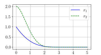
Figure 1: Simulation results for Example 1 (cascade interconnection).

V-B Example 2: Feedback Interconnection

Consider the feedback interconnection of two systems as shown below:

• System 1 (with state $[x_{11},x_{12}]^{T}$ and input $u_{1}$):

  $$\dot{x}_{11} =x_{12}+x_{21}^{3}\ \ \ ;\ \ \ \dot{x}_{12}=u_{1}.$$ (33)

• System 2 (with state $[x_{21},x_{22}]^{T}$ and input $u_{2}$):

  $$\dot{x}_{21} =x_{22}+\sin(x_{21})x_{11}\ \ \ ;\ \ \ \dot{x}_{22}=u_{2}.$$ (34)

Consider that we wish to design a decentralized controller (i.e., $u_{1}$ having state dependence only on $[x_{11},x_{12}]^{T}$; $u_{2}$ having state dependence only on $[x_{21},x_{22}]^{T}$) to make the overall interconnected system PT-C. We design prescribed-time controllers for the two systems below using two different control design methods and then show as an application of Theorem 4 that the interconnected system is PT-C.

For the first system, we use a backstepping approach. Define the virtual control law $x_{12}^{*}=-k_{11}\varphi_{1}(t)x_{11}-k_{12}\varphi_{1}(t)x_{11}^{9}$ with $k_{11}$ and $k_{12}$ being positive constants and with $\varphi_{1}(t)$ being a polynomially bounded blow-up function to be picked below. The choice of the term involving $x_{11}^{9}$ is motivated by the fact noted below that the upper bounding of the expression obtained in the Lyapunov analysis from the interconnection term $x_{21}^{3}$ will generate a term involving $x_{11}^{12}$. Then, with $z_{12}=x_{12}-x_{12}^{*}$, we define the Lyapunov function $V_{1}=\frac{1}{4}x_{11}^{4}+\frac{c_{1}}{2}z_{12}^{2}$ with $c_{1}$ being a positive constant. Then, we have

$$\dot{V}_{1} =x_{11}^{3}(x_{12}+x_{21}^{3})+c_{1}z_{12}(u_{1}+\dot{\varphi}_{1}(t)(k_{11}x_{11}+k_{12}x_{11}^{9})$$

$$\quad+\varphi_{1}(t)(k_{11}+9k_{12}x_{11}^{8})(x_{12}+x_{21}^{3})).$$ (35)

Using the inequality $ab\leq\frac{1}{p}|a|^{p}+\frac{1}{q}|b|^{q}$ which holds for any real numbers $a$ and $b$ and any positive constants $p$ and $q$ with $\frac{1}{p}+\frac{1}{q}=1$, we can write the following inequalities to upper bound the various “interconnection” terms (i.e., terms involving state variables of both System 1 and System 2) appearing in the right hand side of (35):

$$x_{11}^{3}x_{21}^{3} \leq\frac{3}{4(4\varphi_{1}(t)k_{12})^{\frac{1}{3}}}x_{21}^{4}+k_{12}\varphi_{1}(t)x_{11}^{12}$$ (36)

$$c_{1}z_{12}\varphi_{1}(t)(k_{11}+9k_{12}x_{11}^{8})x_{21}^{3} \leq\frac{3}{4(4\varphi_{1}(t)k_{12})^{\frac{1}{3}}}x_{21}^{4}$$

$$\!\!\!\!\!\!\!\!\!\!\!\!\!\!\!+k_{12}c_{1}^{4}z_{12}^{4}\varphi_{1}^{5}(t)(k_{11}+9k_{12}x_{11}^{8})^{4}.$$ (37)

Designing the control input $u_{1}$ as

$$u_{1} =-k_{13}z_{12}\varphi_{1}(t)-\frac{1}{c_{1}}x_{11}^{3}-\dot{\varphi}_{1}(t)(k_{11}x_{11}+k_{12}x_{11}^{9})$$

$$\quad-\varphi_{1}(t)(k_{11}+9k_{12}x_{11}^{8})x_{12}$$

$$\quad-k_{12}c_{1}^{3}z_{12}^{3}\varphi_{1}^{5}(t)(k_{11}+9k_{12}x_{11}^{8})^{4}$$ (38)

with $k_{13}$ being a positive constant, and using the inequalities (36) and (37), (35) reduces to

$$\dot{V}_{1} \leq-k_{11}\varphi_{1}(t)x_{11}^{4}-k_{13}\varphi_{1}(t)c_{1}z_{12}^{2}+\frac{3}{2(4\varphi_{1}(t)k_{12})^{\frac{1}{3}}}x_{21}^{4}.$$ (39)

To design the controller for the second system (i.e., the system with state variables $[x_{21},x_{22}]^{T}$), we apply a high-gain scaling analogous to [9, 10], but with a polynomially bounded blow-up function $\varphi_{2}(t)$ in place of a dynamic high-gain scaling parameter $r$:

$$\overline{x}_{21} =x_{21}\ ;\ \overline{x}_{22}=\frac{x_{22}}{\varphi_{2}(t)}.$$ (40)

In terms of these scaled state variables, we have the dynamics

$$\dot{\overline{x}}_{21} =\varphi_{2}(t)\overline{x}_{22}+\sin(\overline{x}_{21})x_{11}$$

$$\dot{\overline{x}}_{22} =-\frac{\dot{\varphi}_{2}(t)}{\varphi_{2}(t)}\overline{x}_{22}+\frac{1}{\varphi_{2}(t)}u_{2}.$$ (41)

Defining the Lyapunov function of form

$$V_{2} =\frac{1}{4}\overline{x}_{21}^{4}+\frac{c_{2}}{2}(\overline{x}_{22}+k_{21}\overline{x}_{21})^{2}$$ (42)

with $k_{21}$ being a positive constant, we obtain

$$\dot{V}_{2} =\overline{x}_{21}^{3}(\varphi_{2}(t)z_{22}-\varphi_{2}(t)k_{21}\overline{x}_{21}+\sin(\overline{x}_{21})x_{11})$$

$$\quad+c_{2}z_{22}\Big{(}-\frac{\dot{\varphi}_{2}(t)}{\varphi_{2}(t)}\overline{x}_{22}+\frac{1}{\varphi_{2}(t)}u_{2}$$

$$\quad+k_{21}(\varphi_{2}(t)\overline{x}_{22}+\sin(\overline{x}_{21})x_{11})\Big{)}$$ (43)

where $z_{22}=\overline{x}_{22}+k_{21}\overline{x}_{21}$. We can write the following inequalities to upper bound the various interconnection terms appearing in the right hand side of (43):

$$\overline{x}_{21}^{3}\sin(\overline{x}_{21})x_{11} \leq\frac{1}{4}\varphi_{2}(t)k_{21}\overline{x}_{21}^{4}+\frac{27}{4(\varphi_{2}(t)k_{21})^{3}}x_{11}^{4}$$ (44)

$$c_{2}z_{22}k_{21}\sin(\overline{x}_{21})x_{11} \leq\frac{1}{2}c_{2}^{2}k_{21}^{2}z_{22}^{2}+\frac{1}{4}\varphi_{2}(t)k_{21}\overline{x}_{21}^{4}+$$

$$\quad\frac{1}{4\varphi_{2}(t)k_{21}}x_{11}^{4}.$$ (45)

Designing the control input $u_{2}$ as

$$u_{2} =-\dot{\varphi}_{2}(t)k_{21}\overline{x}_{21}+\varphi_{2}(t)\Big{(}-k_{21}\varphi_{2}(t)\overline{x}_{22}-\frac{1}{c_{2}}\varphi_{2}(t)\overline{x}_{21}^{3}$$

$$\quad-\frac{1}{2}c_{2}k_{21}^{2}z_{22}-\varphi_{2}(t)k_{22}z_{22}\Big{)}$$ (46)

with $k_{22}$ being a positive constant, using the inequalities (44) and (45), and noting that $\dot{\varphi}_{2}(t)$ is non-negative for any blow-up function $\varphi_{2}$, (43) reduces to

$$\dot{V}_{2} \leq-\frac{1}{2}\varphi_{2}(t)k_{21}\overline{x}_{21}^{4}-k_{22}\varphi_{2}(t)c_{2}z_{22}^{2}$$

$$\quad+\Big{(}\frac{27}{4(\varphi_{2}(t)k_{21})^{3}}+\frac{1}{4\varphi_{2}(t)k_{21}}\Big{)}x_{11}^{4}.$$ (47)

Denoting $\varphi_{10}=\varphi_{1}(0)$ and $\varphi_{20}=\varphi_{2}(0)$, we see from (39) and (47) that inequalities of the form (19) and (20) are satisfied with $a_{1}=\min(4k_{11},2k_{13})$, $a_{2}=\min(2k_{21},2k_{22})$, $b_{1}=\frac{6}{\varphi_{10}(4\varphi_{10}k_{12})^{\frac{1}{3}}}$, and $b_{2}=\frac{27}{\varphi_{20}(\varphi_{20}k_{21})^{3}}+\frac{1}{\varphi_{20}^{2}k_{21}}$. From Theorem 4, it follows that the feedback interconnection of the two systems is PT-C if the controller parameters are picked such that $a_{1}a_{2}>b_{1}b_{2}$. Note that the control designs for $u_{1}$ and $u_{2}$ in (38) and (46) are based on two different methods and are decentralized in the sense that each control law depends only on the state variables of the corresponding system (i.e., $u_{1}$ is a function of $[x_{11},x_{12}]^{T}$; $u_{2}$ is a function of $[x_{21},x_{22}]^{T}$).

For simulation studies, we pick the blow-up functions for the two systems to be $\varphi_{1}(t)=6+\left(\frac{T}{T-t}\right)^{2}$ and $\varphi_{2}(t)=6+\left(\frac{T}{T-t}\right)^{3}$, respectively. The motivation for including positive constants in the choices of $\varphi_{1}(t)$ and $\varphi_{2}(t)$ is to increase the values of $\varphi_{10}=\varphi_{1}(0)$ and $\varphi_{20}=\varphi_{2}(0)$ taking into account the appearance of these values in the expressions for $b_{1}$ and $b_{2}$ so as to make $b_{1}$ and $b_{2}$ smaller making it more likely that the condition $a_{1}a_{2}>b_{1}b_{2}$ is satisfied. The controller parameters are picked to be $k_{11}=0.25$, $k_{12}=0.1$, $k_{13}=0.5$, $c_{1}=0.05$, $k_{21}=0.25$, $k_{22}=0.5$, and $c_{2}=0.02$. With these choices of the controller parameters, we see that the parameters $a_{1}$, $a_{2}$, $b_{1}$, and $b_{2}$ in (19) and (20) are $a_{1}=1$, $a_{2}=0.5$, $b_{1}=0.608$, and $b_{2}=0.801$. With these parameters, we have $a_{1}a_{2}=0.5$ and $b_{1}b_{2}=0.487$. Hence, the condition $a_{1}a_{2}>b_{1}b_{2}$ is satisfied implying that the feedback interconnection of Systems 1 and 2 is PT-C by Theorem 4.

Simulation results for the closed-loop interconnected system using the control designs described above are shown in Figure 2. The initial conditions for the simulation are specified as $x_{11}=x_{12}=x_{21}=x_{22}=1$. As in Example 1, the prescribed time $T$ is set to be 5 s and the effective terminal time $\overline{T}$ to avoid numerical issues in simulations is set to be $\overline{T}=5.05$. It is seen that all the state variables as well as the control inputs converge to 0 as $t\rightarrow T$. Note however that the condition $a_{1}a_{2}>b_{1}b_{2}$ is a sufficient but not necessary condition and furthermore, there is some intrinsic conservativeness in the upper bounds (36), (37), (44), and (45). Hence, the controller parameters could be tuned to reduce overshoots (e.g., picking smaller controller gains such as $k_{11}=k_{21}=0.1$ and removing the additive positive constants in the choices of $\varphi_{1}(t)$ and $\varphi_{2}(t)$ results in smoother closed-loop trajectories with greatly reduced values of the control signals). Simulation plots with these modified controller parameters are omitted for brevity.

In the control designs above, note that $u_{1}$ and $u_{2}$ involve the time derivatives $\dot{\varphi}_{1}(t)$ and $\dot{\varphi}_{2}(t)$, respectively. The convergence of $u_{1}$ and $u_{2}$ to zero inspite of this dependence on the time derivatives of the blow-up functions is due to the fact that these time derivatives $\dot{\varphi}_{1}(t)$ and $\dot{\varphi}_{2}(t)$ are also polynomially bounded blow-up functions. Hence, the terms in $u_{1}$ and $u_{2}$ involving these time derivatives are products of polynomially bounded blow-up functions and prescribed-time exponentially convergent signals and it is known from Lemma 2 that such products are also prescribed-time exponentially convergent (to zero). To see that the time derivatives $\dot{\varphi}_{1}(t)$ and $\dot{\varphi}_{2}(t)$ are also polynomially bounded blow-up functions, note that for any blow-up function $\varphi(t)$ which is a polynomial in $\frac{T}{T-t}$, its time derivative $\dot{\varphi}(t)$ is also a polynomial in $\frac{T}{T-t}$ since $\frac{d}{dt}\left(\frac{T}{T-t}\right)^{a}=\frac{a}{T-t}\left(\frac{T}{T-t}\right)^{a}$ for any $a\geq 1$. Hence, $\dot{\varphi}(t)$ is also a polynomially bounded blow-up function.

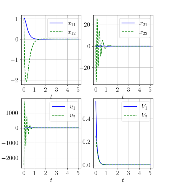
Figure 2: Simulation results for Example 2 (feedback interconnection).

VI Conclusion

Cascade and feedback interconnections of prescribed-time ISS systems were considered and sufficient conditions were developed under which such interconnections retain prescribed-time convergence properties. Interconnections both of two systems and of an arbitrary number of systems were considered. Central tools in the analysis were the newly introduced notions of polynomially bounded blow-up functions and prescribed-time exponential convergence and the related concept of prescribed-time exponentially convergent Lyapunov certificates. A detailed analysis of these new notions was presented and their links to prescribed-time convergence properties of interconnected systems were explored. Simulation studies were performed for example systems in cascade and feedback interconnection structures. In the feedback interconnection example, a scenario where controllers are designed separately for the two systems in the interconnection (indeed, using two different control design methods) was considered and it was shown as an application of the developed theoretical results that the controllers can be put together to achieve prescribed-time stabilization of the interconnected system. The newly introduced notions noted above provide powerful tools for analyzing prescribed-time properties of both single systems and interconnected systems. Future work will address further study of the application of these notions in the context of more general interconnection structures (e.g., general nonlinear and time-varying dependencies in Lyapunov inequalities of each system on Lyapunov certificates of other systems) involving wider classes of nonlinear systems and control designs including adaptive and output-feedback controllers.

References

- [1] Y. Song, Y. Wang, J. Holloway, and M. Krstic, “Time-varying feedback for regulation of normal-form nonlinear systems in prescribed finite time,” Automatica, vol. 83, pp. 243–251, Sept. 2017.
- [2] E. Jiménez-Rodríguez, J. D. Sánchez-Torres, and A. G. Loukianov, “On optimal predefined-time stabilization,” Intl. Jour. of Robust and Nonlinear Control, vol. 27, no. 17, pp. 3620–3642, Nov. 2017.
- [3] D. Tran, T. Yucelen, and B. Sarsilmaz, “Control of multiagent networks as systems: Finite-time algorithms, time transformation, and separation principle,” in Proc. of the IEEE Conf. on Decision and Control, Miami Beach, FL, Dec. 2018, pp. 6204–6209.
- [4] H. M. Becerra, C. R. Vázquez, G. Arechavaleta, and J. Delfin, “Predefined-time convergence control for high-order integrator systems using time base generators,” IEEE Trans. on Control Systems Technology, vol. 26, no. 5, pp. 1866–1873, Sept. 2018.
- [5] Y. Song, Y. Wang, and M. Krstic, “Time-varying feedback for stabilization in prescribed finite time,” Intl. Jour. of Robust and Nonlinear Control, vol. 29, no. 3, pp. 618–633, Feb. 2019.
- [6] J. D. Sánchez-Torres, M. Defoort, and A. J. Muñoz-Vázquez, “Predefined-time stabilisation of a class of nonholonomic systems,” Intl. Jour. of Control, Jan. 2019.
- [7] K. Zhao, Y. Song, and Y. Wang, “Regular error feedback based adaptive practical prescribed time tracking control of normal-form nonaffine systems,” Jour. of the Franklin Institute, vol. 356, no. 5, pp. 2759 – 2779, Mar. 2019.
- [8] P. Krishnamurthy, F. Khorrami, and M. Krstic, “Robust output-feedback prescribed-time stabilization of a class of nonlinear strict-feedback-like systems,” in Proc. of the European Control Conf., Naples, Italy, June 2019, pp. 1148–1153.
- [9] P. Krishnamurthy, F. Khorrami, and M. Krstic, “Prescribed-time stabilization of nonlinear strict-feedback-like systems,” in Proc. of the American Control Conf., Philadelphia, PA, July 2019, pp. 3081–3086.
- [10] P. Krishnamurthy, F. Khorrami, and M. Krstic, “A dynamic high-gain design for prescribed-time regulation of nonlinear systems,” Automatica, vol. 115, p. 108860, May 2020.
- [11] P. Krishnamurthy and F. Khorrami, “Prescribed-time output-feedback stabilization of uncertain nonlinear systems with unknown time delays,” in Proc. of the American Control Conf., Denver, CO, USA, 2020, pp. 2705–2710.
- [12] D. Gómez-Gutiérrez, “On the design of nonautonomous fixed-time controllers with a predefined upper bound of the settling time,” Intl. Jour. of Robust and Nonlinear Control, vol. 30, no. 10, pp. 3871–3885, 2020.
- [13] B. Zhou and Y. Shi, “Prescribed-time stabilization of a class of nonlinear systems by linear time-varying feedback,” IEEE Trans. on Automatic Control, vol. 66, no. 12, pp. 6123–6130, 2021.
- [14] P. Krishnamurthy, F. Khorrami, and M. Krstic, “Adaptive output-feedback stabilization in prescribed time for nonlinear systems with unknown parameters coupled with unmeasured states,” Intl. Jour. of Adaptive Control and Signal Processing, vol. 35, no. 2, pp. 184–202, Feb. 2021.
- [15] C. Hua, P. Ning, and K. Li, “Adaptive prescribed-time control for a class of uncertain nonlinear systems,” IEEE Trans. on Automatic Control, vol. 67, no. 11, pp. 6159–6166, 2022.
- [16] P. Krishnamurthy and F. Khorrami, “Prescribed-time regulation of nonlinear uncertain systems with unknown input gain and appended dynamics,” Intl. Jour. of Robust and Nonlinear Control, vol. 33, no. 5, pp. 3004–3026, 2023.
- [17] B. Zhou and K.-K. Zhang, “A linear time-varying inequality approach for prescribed time stability and stabilization,” IEEE Trans. on Cybernetics, vol. 53, no. 3, pp. 1880–1889, 2023.
- [18] H. Ye and Y. Song, “Prescribed-time control for linear systems in canonical form via nonlinear feedback,” IEEE Trans. on Systems, Man, and Cybernetics: Systems, vol. 53, no. 2, pp. 1126–1135, 2023.
- [19] W. Li and M. Krstic, “Prescribed-time mean-nonovershooting control under finite-time vanishing noise,” SIAM Jour. on Control and Optimization, vol. 61, no. 3, pp. 1187–1212, 2023.
- [20] M. Krstić, I. Kanellakopoulos, and P. V. Kokotović, Nonlinear and Adaptive Control Design. New York: Wiley, 1995.
- [21] A. Isidori, Nonlinear Control Systems II. London, UK: Springer, 1999.
- [22] V. Haimo, “Finite time controllers,” SIAM Jour. on Control and Optimization, vol. 24, no. 4, pp. 760–770, 1986.
- [23] S. P. Bhat and D. S. Bernstein, “Finite-time stability of continuous autonomous systems,” SIAM Jour. on Control and Optimization, vol. 38, no. 3, pp. 751–766, 2000.
- [24] X. Huang, W. Lin, and B. Yang, “Global finite-time stabilization of a class of uncertain nonlinear systems,” Automatica, vol. 41, no. 5, pp. 881–888, May 2005.
- [25] Y. Hong and Z. P. Jiang, “Finite-time stabilization of nonlinear systems with parametric and dynamic uncertainties,” IEEE Trans. on Automatic Control, vol. 51, no. 12, pp. 1950–1956, Dec. 2006.
- [26] S. Seo, H. Shim, and J. H. Seo, “Global finite-time stabilization of a nonlinear system using dynamic exponent scaling,” in Proc. of the IEEE Conf. on Decision and Control, Cancun, Mexico, Dec. 2008, p. 3805–3810.
- [27] E. Moulay and W. Perruquetti, “Finite time stability conditions for non-autonomous continuous systems,” Intl. Jour. of Control, vol. 81, pp. 797–803, 2008.
- [28] Y. Shen and Y. Huang, “Global finite-time stabilisation for a class of nonlinear systems,” Intl. Jour. of Systems Science, vol. 43, no. 1, pp. 73–78, 2012.
- [29] Z. Y. Sun, L. R. Xue, and K. M. Zhang, “A new approach to finite-time adaptive stabilization of high-order uncertain nonlinear system,” Automatica, vol. 58, pp. 60–66, Aug. 2015.
- [30] V. Andrieu, L. Praly, and A. Astolfi, “Homogeneous approximation, recursive observer design, and output feedback,” SIAM Jour. on Control and Optimization, vol. 47, no. 4, pp. 1814–1850, 2008.
- [31] A. Polyakov, “Nonlinear feedback design for fixed-time stabilization of linear control systems,” IEEE Trans. on Automatic Control, vol. 57, no. 8, pp. 2106–2110, Aug. 2012.
- [32] A. Polyakov, D. Efimov, and W. Perruquetti, “Robust stabilization of MIMO systems in finite/fixed time,” Intl. Jour. of Robust and Nonlinear Control, vol. 26, no. 1, pp. 69–90, Jan. 2016.
- [33] K. Zimenko, A. Polyakov, D. Efimov, and W. Perruquetti, “On simple scheme of finite/fixed-time control design,” Intl. Jour. of Control, Aug. 2018.
- [34] R. Aldana-López, D. Gómez-Gutiérrez, E. Jiménez-Rodríguez, J. D. Sánchez-Torres, and M. Defoort, “Enhancing the settling time estimation of a class of fixed-time stable systems,” Intl. Jour. of Robust and Nonlinear Control, vol. 29, no. 12, pp. 4135–4148, Aug. 2019.
- [35] Y. Song, H. Ye, and F. L. Lewis, “Prescribed-time control and its latest developments,” IEEE Trans. on Systems, Man, and Cybernetics: Systems, vol. 53, no. 7, pp. 4102–4116, 2023.
- [36] P. Krishnamurthy and F. Khorrami, “Dynamic high-gain scaling: state and output feedback with application to systems with ISS appended dynamics driven by all states,” IEEE Trans. on Automatic Control, vol. 49, no. 12, pp. 2219–2239, Dec. 2004.
- [37] P. Krishnamurthy and F. Khorrami, “On uniform solvability of parameter-dependent Lyapunov inequalities and applications to various problems,” SIAM Jour. of Control and Optimization, vol. 45, no. 4, pp. 1147–1164, 2006.
- [38] P. Krishnamurthy and F. Khorrami, “Dual high-gain-based adaptive output-feedback control for a class of nonlinear systems,” Intl. Jour. of Adaptive Control and Signal Processing, vol. 22, no. 1, pp. 23–42, 2008.
- [39] P. Krishnamurthy and F. Khorrami, “A general dynamic scaling based control redesign to handle input unmodeled dynamics in uncertain nonlinear systems,” IEEE Trans. on Automatic Control, vol. 62, no. 9, pp. 4719–4726, Sep. 2017.
- [40] P. Krishnamurthy, F. Khorrami, and M. Krstic, “Robust adaptive prescribed-time stabilization via output feedback for uncertain nonlinear strict-feedback-like systems,” European Jour. of Control, vol. 55, pp. 14–23, Sept. 2020.
- [41] E. D. Sontag, “On the input-to-state stability property,” European Jour. of Control, vol. 1, no. 1, pp. 24–36, 1995.
- [42] Y. Hong, Z.-P. Jiang, and G. Feng, “Finite-time input-to-state stability and applications to finite-time control design,” SIAM Jour. on Control and Optimization, vol. 48, no. 7, pp. 4395–4418, 2010.
- [43] F. Lopez-Ramirez, D. Efimov, A. Polyakov, and W. Perruquetti, “Finite-time and fixed-time input-to-state stability: Explicit and implicit approaches,” Systems and Control Letters, vol. 144, p. 104775, 2020.
- [44] K.-K. Zhang, B. Zhou, and G.-R. Duan, “Prescribed-time input-to-state stabilization of normal nonlinear systems by bounded time-varying feedback,” IEEE Trans. on Circuits and Systems I: Regular Papers, vol. 69, no. 9, pp. 3715–3725, 2022.
- [45] Z.-P. Jiang, I. M. Mareels, and Y. Wang, “A Lyapunov formulation of the nonlinear small-gain theorem for interconnected ISS systems,” Automatica, vol. 32, no. 8, pp. 1211–1215, 1996.
- [46] G. P. Barker, A. Berman, and R. J. Plemmons, “Positive diagonal solutions to the Lyapunov equations,” Linear and Multilinear Algebra, vol. 5, no. 4, pp. 249–256, 1978.
- [47] A. Berman and D. Hershkowitz, “Matrix diagonal stability and its implications,” Siam Jour. on Algebraic and Discrete Methods, vol. 4, pp. 377–382, 09 1983.
- [48] J. Kraaijevanger, “A characterization of Lyapunov diagonal stability using Hadamard products,” Linear Algebra and its Applications, vol. 151, pp. 245–254, 1991.
- [49] S. Jain and F. Khorrami, “Robust adaptive control of a class of nonlinear systems: state and output feedback,” in Proc. of the American Control Conf., Seattle, WA, June 1995, pp. 1580–1584.
- [50] P. Krishnamurthy and F. Khorrami, “Robust adaptive control for non-linear systems in generalized output-feedback canonical form,” Intl. Jour. of Adaptive Control and Signal Processing, vol. 17, no. 4, pp. 285–311, May 2003.
- [51] R. Bellman, Stability Theory of Differential Equations. New York, USA: McGraw-Hill, 1953.
- [52] B. G. Pachpatte, Inequalities for Differential and Integral Equations. San Diego, USA: Academic Press, 1998.