Optimized Distribution of Entanglement Graph States in Quantum Networks

Abstract

Building large-scale quantum computers, essential to demonstrating quantum advantage, is a key challenge. Quantum Networks (QNs) can help address this challenge by enabling the construction of large, robust, and more capable quantum computing platforms by connecting smaller quantum computers. Moreover, unlike classical systems, QNs can enable fully secured long-distance communication. Thus, quantum networks lie at the heart of the success of future quantum information technologies. In quantum networks, multipartite entangled states distributed over the network help implement and support many quantum network applications for communications, sensing, and computing. Our work focuses on developing optimal techniques to generate and distribute multipartite entanglement states efficiently.

Prior works on generating general multipartite entanglement states have focused on the objective of minimizing the number of maximally entangled pairs (EPs) while ignoring the heterogeneity of the network nodes and links as well as the stochastic nature of underlying processes. In this work, we develop a hypergraph-based linear programming framework that delivers optimal (under certain assumptions) generation schemes for general multipartite entanglement represented by graph states, under the network resources, decoherence, and fidelity constraints, while considering the stochasticity of the underlying processes. We illustrate our technique by developing generation schemes for the special cases of path and tree graph states, and discuss optimized generation schemes for more general classes of graph states. Using extensive simulations over a quantum network simulator (NetSquid), we demonstrate the effectiveness of our developed techniques and show that they outperform prior known schemes by up to orders of magnitude.

I Introduction

Quantum networks (QNs) enable the construction of large-scale and robust quantum computing platforms by connecting smaller QCs [1]. QNs also enable various important applications [2, 3, 4, 5, 6, 7, 8, 9], but to implement and support many of these applications, we need to create and distribute entangled states efficiently. Recent works have addressed the generation of entanglement states but in limited settings, e.g., bipartite and GHZ states, or graph states with a simplistic optimization objective. In this paper, we consider the generation and distribution of specialized graph states over quantum networks, with minimal generation latency, taking into consideration the stochastic nature of the underlying generation process.

Graph States and Their Applications. Graph states are multipartite entangled states where a graph over the qubits specifies the entanglement structure between qubits. Owing to their highly entangled nature, graph states find applications in various quantum information processing domains, such as measurement-based quantum computing, quantum error correction, quantum secret sharing, and quantum metrology. In particular, path/cycle graph states are used as a primary resource state of fusion-based quantum computing [10], and tree graph states find usage in counterfactual error correction [11], photonic measurement-based quantum computing, and fusion-based quantum computing [10]. The star graph state, which is a special case of a tree graph state, is equivalent to a GHZ state—which has many applications, including error correction [11], quantum secret sharing [12], quantum metrology [13], clock synchronization [5], etc. Therefore, developing efficient generation schemes to distribute graph states in a QN is of great significance. Our work focuses on developing optimal generation schemes for general classes of graph states.

Prior Work and Our Approach. There have been recent works [14, 15, 16] that have addressed the problem of efficient generation and distribution of general graph state entanglements in a quantum network. These works, however, have focused on the simplistic optimization objective of minimizing the number of maximally entangled pairs (e-bits or EPs) consumed; in particular, they implicitly ignore the stochastic nature of the underlying processes. Even a true count of EPs consumed should consider the stochastic nature of operations (e.g., fusion) involved, particularly since they can have a relatively low probability of success. Moreover, some EPs may take significantly longer to generate than others due to the heterogeneity of the network. Thus, the number of EPs is too simplistic a performance metric.

In this work, we consider the generation and distribution of classes of graph states to maximize the expected generation rate under given network resource and fidelity constraints while considering the stochastic nature of underlying processes and network heterogeneity. This is in the same vein as the recent works on the generation of EPs [17, 18, 19, 20] and GHZ states [21] in quantum networks. In particular, our goal is to develop provably optimal generation schemes. We develop a framework—based on a hypergraph representation of the intermediate graph states and fusion operations—that delivers optimal (under reasonable assumptions) generation schemes under network and fidelity constraints. We illustrate our framework by developing multiple generation schemes for the path and tree graph states, and discuss generalizations to other classes of graphs. In essence, our proposed schemes use fusion operations to build larger graph states from smaller ones progressively and discover the optimal level-based structure (that represents the generation process, i.e., sequence and order of fusion operations over intermediate graph states) by using an appropriate linear programming (LP) formulation.

Our Contributions. In the above context, we make the following contributions.

1. We develop a framework for developing optimal schemes for generating graph states in quantum networks under network resource and fidelity constraints, considering the stochastic nature of the fusion operations.

2. Specifically, for path graph states, we design a polynomial-time generation scheme that is provably optimal under reasonable assumptions. In addition, we also develop an optimal two-stage generation scheme that is computationally more efficient, based on restricting the intermediate graph states created.

3. Similarly, for tree graph states, we design two generation schemes that are optimal under the restriction on the intermediate states and fusion operations used.

4. We show the versatility of our developed scheme by discussing and illustrating its application for other classes of graph states, e.g., grid graphs, bipartite graphs, and complete graphs. We also generalize our scheme to generate multiple graph states concurrently.

5. Using extensive evaluations over the NetSquid simulator, we demonstrate the effectiveness of our developed techniques and show that they outperform prior work by up to orders of magnitude.

II Background

Quantum Network (QN), Nodes, Links, and Communication. A quantum network (QN) is a network of quantum computers (QCs), and is represented as a connected undirected graph with vertices as QCs and edges representing the (quantum and classical) direct communication links. We use network nodes and links to refer to the vertices (QCs) and edges in the QN graph. We discuss a detailed network model in §III. Since direct transmission of quantum data is subject to unrecoverable errors, especially over long distances, we use teleportation to transfer quantum information reliably across nodes in a QN. Teleportation requires that a maximally-entangled pair (EP) be already established over communicated nodes.

Generation of Remote EPs using Swapping Trees. An efficient way to generate an EP over a pair of remote network nodes $(s,d)$ using EPs over network links (i.e., edges) is to: (i) create a path $P$ in the network graph from $s$ to $d$ with EPs over each of the paths’ edges, and (ii) perform a series of entanglement swaps (ES) over these EPs. The series of ES operations over $P$ can be performed in any arbitrary order, but this order of ES operations affects the latency incurred in generating the EP over $(s,d)$. One way to represent the “order” in which the ES operations are executed—is a complete binary tree over the link EPs as leaves, called a swapping tree [17]. The stochastic nature of ES operations entails that generation of an EP over a remote pair of nodes using a swapping tree may incur significant latency, called the generation latency (inverse of generation rate). Generation latency is largely due to the latency incurred in (i) generating the link EPs, and (ii) a generated EP $(x_{i},x_{j})$ waiting for its ”sibling” EP $(x_{j},x_{k})$ to be generated before an ES operation can be performed over them to generate an EP over $(x_{i},x_{k})$.

II-A Multipartite Entanglements

Distributed Graph States; Link States. A graph state is a multi-partite quantum state $|G\rangle$ which is described by a graph $G$, where the vertices of G correspond to the qubits of $|G\rangle$. Formally, a graph state $|G\rangle$ is given as

$$|G\rangle=\Pi_{(u,v)\in E(G)}C_{Z}^{(u,v)}\otimes_{v\in V(G)}|+\rangle_{v},$$

where $C_{Z}^{(u,v)}$ is the controlled-Z (CZ) gate over the qubits $u$ and $v$. We use the term distributed graph state to mean a graph state $G$ along with its (target or current) distribution over the given quantum network; this distribution is represented by a function $\tau:V(G)\mapsto V(Q)$ of graph state’s vertices $V(G)$ to the nodes $V(Q)$ in the given quantum network $Q$. For brevity, when clear from the context, we just use states to refer to distributed graph states. Also, we use the term link states to refer to the single-edge graph states distributed over the network links; these link states are locally equivalent to the link-EPs generated by the adjacent nodes.

Generating of Graph States via Fusion Trees. We need to fuse smaller graph states and/or modify graph states to generate general graph states. In general, starting with link states, we want to generate graph states using only local quantum operations (i.e., gates with operands in a single node). Similar to swapping trees used to describe the generation of EPs, we can use fusion trees to describe the generation of graph states in a QN using fusion operations. Each node in a fusion tree would represent a distributed graph state. Such fusion trees have been used in prior works—e.g., for generating and distributing GHZ states [21].

Fusion Operations. Local operations within a fusion are generally restricted to single-qubit Clifford operations, local CZ gates, or Pauli measurements. In our context, we only use the following local operations or measurements within a fusion:

1. Create or remove an edge by doing a CZ over two qubits in a single node.

2. Pauli-Y measurement over a qubit/vertex $q$ results in a local complementation of vertex $q$’s neighborhood and then $q$’s deletion, while Pauli-Z measurement over a qubit $q$ results in $q$’s deletion.

3. Also, one can effectuate local complementation of any vertex $q$ by doing local single-qubit Clifford Operations.

III Model, Problem, and Related Works

In this section, we discuss our network model, formulate the problem addressed, and discuss related work.

Network Model. We denote a quantum network (QN) $Q$ with $V(Q)$ denoting the set of nodes. Adjacent nodes signify nodes connected by a communication link. Our network model is similar to the one used in some of the recent works [17, 21] on efficient generation of EPs and GHZ states. In particular, each node has an atom-photon EP generator with generation latency ($t_{g}$) and probability of success ($p_{g}$); the atom-photo generation latency implicitly includes other latencies incurred in link EP generation viz. photon transmission, optical-BSM, and classical acknowledgment. A node’s atom-photon generation capacity/rate is its aggregate capacity and may be split across its incident links. Each network link $e=(A,B)$ is used to generate link-EPs, using an optical-BSM device located in the middle. The optical-BSM has a certain probability of success ($p_{ob}$), and each half-link (from $A$ or $B$) to the device has a probability of transmission success ($p_{e}$) that decreases exponentially with the link distance. To facilitate atom-atom ES and fusion operations, each network node is also equipped with an atomic-BSM device with appropriate latency and probability of success. There is an independent classical network with a transmission latency of $t_{c}$; we assume classical transmission always succeeds.

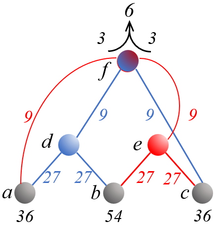
Figure 1: Level-based structure. The above structure is an “aggregation” of two swapping trees. The leaf node $a$’s generation rate of 36 units is “split” into 9 and 27 for the two different (red and blue) fusion operations. The root node represents the final/target graph state formed in two different ways—for a total generation rate of 6 (3 from each fusion operation). We assume that a parent’s generation rate is 1/3 of the rate of its children/operands (which are equal).

Level-Based Fusion Structure. To maximize the generation rate of a graph state, multiple concurrent fusion trees may be required to use all available network resources. Since the number of such trees can be exponential, we use a novel “aggregated” structure that aggregates multiple (fusion) trees into one structure; we refer to this as a level-based structure, as it is composed of multiple levels—with each level consisting of distributed graph states (as vertices) created by fusing states from the previous levels. See Fig. 1. The bottom level consists of link states, and each non-leaf state $S$ is formed by a fusion of pairs of states in the previous layers; however, there may be several such pairs of states that fuse to create $s$ (in different ways). Each state $S$ may also have multiple “parents” (unlike in a tree), i.e., a state $S$ may be used to create several states in the next layer; in such a case, the generation rate of $S$ is “split” across these fusions. Due to the fusions from previous layers, each vertex/state has a resulting generation rate, estimated as discussed below.

Graph State Generation Latency/Rate. The expression for estimating the generation rate (or latency) of a state due to a fusion operation in our level-based structure is fundamentally the same as that used in fusion/swapping trees in prior works [17, 21]. Consider a simple case of a non-leaf node $t$ with two children $t_{l}$ and $t_{r}$ which are fused to generate $t$. If the generation events of the children states $t_{l}$ and $t_{r}$ are Poisson distributed and thus generation latencies are exponentially distributed, then, the generation latency of the graph state corresponding to $t$ can be estimated as (see [17]):

$$L_{t}=(\frac{3}{2}\max(L_{l},L_{r})+\mbox{$t_{f}$}+\mbox{$t_{c}$})/\mbox{$p_{f}$},$$ (1)

where $L_{l}$ and $L_{r}$ are the generation latencies of the graph states corresponding to the children $t_{l}$ and $t_{r}$, $t_{f}$ and $p_{f}$ are the latency and probability of success of the swapping/fusion operation, and $t_{c}$ is the classical transmission latency. The generation rate $G_{t}$ can thus also be estimated as $G_{t}=2/3\min(G_{l},G_{r})$, where $G_{t}$, $G_{l}$, and $G_{r}$ are the generation rates of the nodes. For a state $t$ generated from multiple pairs of children, we take the sum of the generation rates due to each pair. The generation rate of the leaf vertices (link states) in a level-based structure is given by the generation rate of the EP at the network link. To estimate the generation rate of other states in the structure, we apply the above equation iteratively (for this, we implicitly assume that the resulting latencies also have an exponential distribution).

III-A Problem Formulation

In this section, we formulate the problem of efficiently generating distributed graph states over a quantum network. Informally, the problem is to generate the level-based structure with a maximum generation output rate, given the constraints of the nodes’ link-EP generation capacity.

Graph State Generation (GSG) Problem. Given a quantum network $Q$, a graph state $G$ along with its distribution $\tau:V(G)\mapsto V(Q)$, the GSG problem is to determine a level-based structure $\mathcal{F}$ that generates the giving distributed graph state with the optimal (highest) generation rate under the following constraints.

1. Node Constraints. For each network node, the aggregate resources used by $\mathcal{F}$ is less than the available resources; we formulate this formally below.

2. Fidelity Constraints. The structure $\mathcal{F}$ should satisfy the following: (a) The Number of “leaves” of any ”tree” in the level-based structure is less than a given threshold $\tau_{l}$; this is to limit fidelity degradation due to gate operations. (b) Any qubit’s total memory storage time is less than a given decoherence threshold $\tau_{d}$.

We refer to the given $G$ as the target graph state, and the network nodes $\tau(i)$, for $i\in[1,n]$, as the terminal nodes.

Formulating Node Constraints. Consider a level-based structure $\mathcal{F}$. Let $\mathcal{E}$ be the set of all network links, and $\mathcal{E}(i)\subseteq\mathcal{E}$ as the set of links incident on node $i$. For each link $e\in\mathcal{E}$, let $R(e)$ be the total generation rate of $e$ in $\mathcal{F}$. Then, the node capacity constraint is formulated as follows.

$$1/\mbox{$t_{g}$} \geq \sum_{e\in\mathcal{E}(i)}R(e)/(\mbox{$p_{g}$}^{2}\mbox{$p_{e}$}^{2}\mbox{$p_{ob}$})\ \ \ \ \forall i\in V.$$ (2)

The above comes from the fact that to generate an edge graph state over $e$, each end-node of $e$ needs to generate $1/(\mbox{$p_{g}$}^{2}\mbox{$p_{e}$}^{2}\mbox{$p_{ob}$})$ photons successfully, and that $1/\mbox{$t_{g}$}$ is a node’s total generation capacity.

III-B Related Works

There has been recent interest in developing schemes for generating multipartite graph states in a quantum network. Most of these works have focused on minimizing the number of link EPs consumed in generating the graph states. To the best of our knowledge, there has been no prior work on efficient generation of arbitrary graph states (or broad classes of graphs) that optimize the generation rates while taking into considering the stochastic nature of the underlying processes; perhaps, the only exception is [21] which considers the generation of GHZ states (we discuss this below).

Centralized Schemes. In a centralized generation scheme, an appropriately chosen central node first creates the target graph state locally and then teleports qubits to the terminal nodes using EPs. In particular, [15] proposes a max-flow-based approach to minimize the number of link-EPs consumed in generating a graph state using such a scheme. They represent the teleportation routes as multi-path flows and use a network flow approach to maximize the total generation rate. The network-flow approach allows the representation of network resource constraints but ignores the stochastic aspect of the teleportation (or entanglement-swapping) process, which fundamentally requires considering the length of the teleportation paths (ignored in the network-flow representation).

Distributed Schemes. In a distributed generation scheme, the target graph state is generated in a distributed manner (perhaps by iteratively merging smaller graph states)—as in the schemes discussed in this paper. In [14], the authors propose a star expansion operation/sub-protocol to fuse EPs, and use the operation iteratively to generate a target GHZ (equivalent to a star graph) state. Then, using a succession of such star graphs, they create a complete graph state with appropriate edges “decorated”—which are removed to yield the target graph state. Their optimization objective is the minimization of the number of EPs consumed, and more importantly, for sparse graph states, their scheme can be very wasteful. In a more recent work, [16] presents a graph-theoretic strategy to optimize the fusion-based generation of arbitrary graph states effectively; their strategy comprises three stages: simplifying the graph state, building a fusion tree/network, and determining the order of fusions. They use 3-qubit GHZ states as the basic resource and optimize the number of these states used. They do not discuss techniques to generate and distribute graph states over a quantum network; nevertheless, we believe theirs is the most promising approach among existing works for generating arbitrary graph states in a quantum network. Thus, we adapt/extend their scheme for distributing graph states in a quantum network and compare it to our schemes in VIII.

Generating EPs and GHZ States; Our Work. Finally, there have been works on the generation and distribution of specialized graph states, e.g., EPs [17, 18, 19] and GHZ states [21, 22, 23]. Our work on generating general graph states uses a similar network model and optimization formulation as [17, 21], but has different objectives and thus uses different techniques. In particular, [17] designs a dynamic programming approach to construct optimal swapping trees to generate remote EPs, and [21] develops heuristics to construct fusion trees to generate GHZ states. Instead, our objective is to develop a general framework for the optimal generation of general classes of graph states; in particular, we develop a hypergraph-based framework to construct optimal level-based structures (instead of trees) by determining an optimal hyperflow in hypergraphs.

IV High-Level Approach

Here, we discuss our overall approach to optimally solving the GSG problem using linear programming (LP). In the following sections, we will apply our technique to two special cases of graph states: paths and trees. In §VII, we briefly also discuss other classes of graph states to demonstrate the versatility of our approach.

Basic Idea: Given a quantum network and a target graph state, we create a hypergraph that has embedded in it all possible level-based structures. In this envisioned hypergraph, (i) each vertex is a potential intermediate distributed graph state, (ii) each hyperedge ($\{s_{1},s_{2}\},s_{3}$), for vertices $s_{1},s_{2},s_{3}$, is a fusion operation that fuses graph states $s_{1}$ and $s_{2}$ to create $s_{3}$, (iii) a “hyperpath” is a potential fusion tree, (iv) and a hyperflow (i.e., “combination” of hyperpaths) is a level-based structure. To determine the optimal hyperflow (and thus, an optimal level-based structure), we assign flow variables representing generation rates to the hyperedges and create an LP with linear constraints corresponding to network resource constraints, flow conservation, and fusion success probability.

Key Challenge. In general, any distributed graph state in a given network can be considered as an intermediate state in the process of generating a given target graph state; thus, the number of potential intermediate states is exponential ($O(4^{n})$) in the number $n$ of network nodes. However, only certain types of intermediate state are likely to be useful/relevant in the generation of a given target state; e.g., to generate a single-edge graph state, it seems reasonable to consider only single-edge graph states as intermediate states (as in the generation of remote EPs via entanglement swapping, which generates only EPs as intermediate states; note that EPs are locally equivalent to single-edge states). Thus, the key challenge in using the above approach is to determine an appropriate set of intermediate states such that the resulting LP over the corresponding hypergraph is computationally feasible and delivers a “good” solution. In particular, we also consider the below two-stage approach to minimize the number of intermediate states considered.

Two-Stage LP Approaches. One strategy we consider to minimize the number of intermediate states considered is to generate the target graph state in two stages: (i) Generate single-edge graph states for each edge in the target graph state $G$; (ii) Use these edge graph states to iteratively generate appropriate intermediate states and eventually the target graph state; in this second stage, only the terminal nodes are involved. We discuss such approaches for path and tree graph states in the following sections.

V Generating Path Graph States

In this section, we design algorithms to generate distributed path graph states based on the high-level approach described above. We recall the standard hypergraph notion.

Definition 1

(Hypergraph) A directed hypergraph $H=(V(H),E(H))$ has a set of vertices $V(H)$ and a set of (directed) hyperedges $E(H)$, where each hyperedge $e$ is a pair $(t(e),h)$ with the tail $t(e)\subset V(H)$ and the head $h\in(V(H)-t(e))$. $\Box$

V-A Optimal Generation of Path Graph States

Consider a GSG problem instance, wherein the target graph state $G$ is a path graph $(1,2,3\ldots,n)$ with edges $(i,i+1)$ for all $1\leq i<n$ and the target distribution represented by $\tau:V(G)\mapsto V(Q)$.

Basic Idea. For the path state, we hypothesize that the type of intermediate states that can potentially be useful in generating and distributing the path state $G$ are connected subgraphs of $G$ augmented with two edges at the end, i.e., path states $(x,i,i+1,i+2,\ldots,j,y)$ distributed over $(x,\tau(i),\tau(i+1),\tau(i+2),\ldots,\tau(j),y)$. (See Theorem 1 for the rationale). We use fusion operations sufficient to build the above states iteratively, starting from the basic link states. This set of intermediate states and fusion operations over them–yields the hypergraph used to develop the linear program for the GSG problem. We start by developing the notation used to define the intermediate states above.

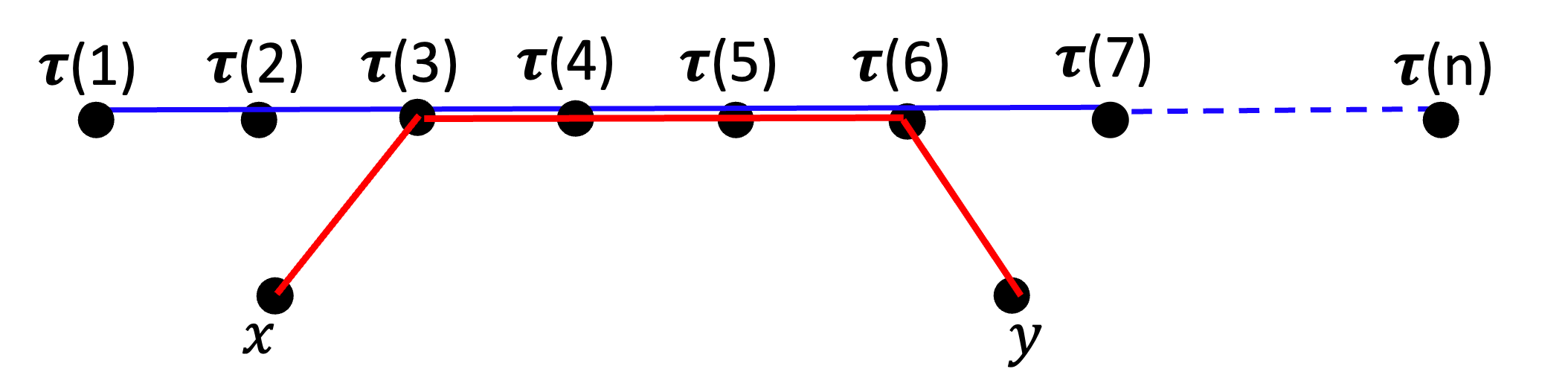
Figure 2: Notation $\langle x,3\cdotp\cdotp 6,y\rangle$ represents a path state $(x,3,4,5,6,y)$ distributed (shown in red) over the network nodes $(x,\tau(3),\tau(4),\tau(5),\tau(6),y)$. The target state $G=(1,2,\ldots,n)$ with distribution function $\tau()$ is in blue.

Notation $\langle x,i\cdotp\cdotp j,y\rangle$. Recall that the target graph state $G$ is a path state $(1,2,3\ldots,n)$ with the distribution function $\tau()$. We use the notation $\langle x,i\cdotp\cdotp j,y\rangle$, where $1\leq i\leq j\leq n$ and $x,y$ are vertices in the QN, to represent the path state $(x,i,i+1,i+2,\ldots,j,y)$ distributed over the network nodes $(x,\tau(i),\tau(i+1),\tau(i+2),\ldots,\tau(j),y)$. See Fig. 2. The above notation is versatile: $i$ may be equal to $j$, signifying a path graph state $(x,i,y)$; or, the middle parameter $i\cdotp\cdotp j$ may be null ($\phi$), signifying an edge graph state $(x,y)$; or, $x$ and/or $y$ may be null. To avoid duplicates, we enforce that if $i=j$ or $i\cdotp\cdotp j$ is $\phi$, then $\tau^{\prime}(x)\leq\tau^{\prime}(y)$.

Intermediate States. As mentioned above, for a given target path graph state $(1,2,\ldots,n)$, we choose the following set of (distributed) intermediate states: $\langle x,i\cdotp\cdotp j,y\rangle$ with $i,j\in[1,n]$, and $x$ and $y$ being any network nodes. Thus, the total number of intermediate states is approximately $n^{2}|V(Q)|^{2}$.

Fusion-Retain and Fusion-Discard Operations. We use fusion operations, viz., fusion-discard and fusion-retain, to manipulate path graph states. The fusion-discard operation merges path graph states $(a_{1},a_{2},\ldots,a_{n})$ and $(b_{1},b_{2},\ldots,b_{m})$ to create $(a_{1},a_{2},\ldots,a_{n-1},b_{2},b_{3},\ldots,b_{m})$, if $a_{n}$ and $b_{1}$ are mapped to (i.e., reside at) the same network node. The fusion-retain operation merges path graph states $(a_{1},a_{2},\ldots,a_{n})$ and $(b_{1},b_{2},\ldots,b_{m})$ to create $(a_{1},a_{2},\ldots,a_{n},b_{2},b_{3},\ldots,b_{m})$, if $a_{n}$ and $b_{1}$ are mapped to the same network node. See Fig. 3, which also shows the local operations used in fusion-retain (we omit details of other fusions).

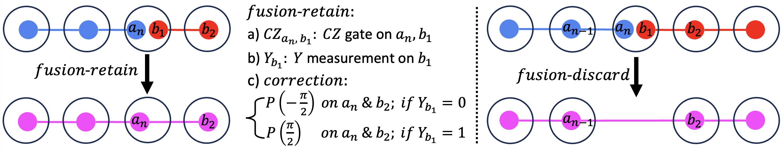
Figure 3: Fusion-retain and Fusion-discard operations.

Hypergraph. We now construct a hypergraph with the above intermediate states as vertices, with the fusion operations over these vertices yielding the hyperedges, as formally described below. Such a hypergraph embeds all level-based structures that represent a generation of the given target graph state.

Hypergraph Vertices. The hypergraph consists of the following vertices.

1. Two distinguished vertices start and term.

2. $Avail(x,i\cdotp\cdotp j,y)$ for each intermediate state $\langle x,i\cdotp\cdotp j,y\rangle$.

3. $Prod^{r}(x,i\cdotp\cdotp j,y)$, and $Prod^{d}(x,i\cdotp\cdotp j,y)$ vertices for the $Avail(x,i\cdotp\cdotp j,y)$ network nodes, as described below.

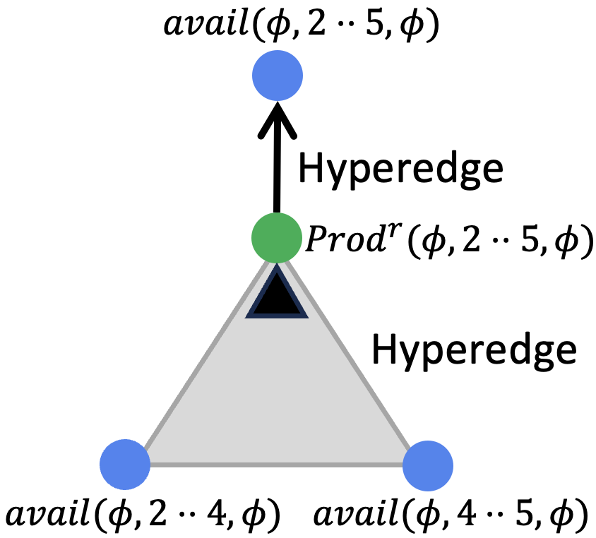
Figure 4: Two hyperedges created to represent a fusion-retain operation.

Hypergraph Edges. The hyperedges should intuitively be of the type $(\{Avail(s_{1}),$ $Avail(s_{2})\}$, $Avail(s_{3}))$, signifying the fusion of states $s_{1}$ and $s_{2}$ to generate $s_{3}$. However, to incorporate the stochasticity of the fusion operations, we create two hyperedges: $(\{Avail(s_{1}),Avail(s_{2})\},Prod^{f}(s_{3}))$ and $(Prod^{f}(s_{3}),Avail(s_{3}))$, where the first edge represents the fusion operation $f$ while the second edge incorporates the fusion’s probability of success (see Eqn. 3). In our context, the superscript $f$ over $Prod()$ is $d$ ($r$) for fusion-discard (fusion-retain). Overall, we have the following set of hyperedges.

1. Hyperedges $(start,avail(x,\phi,y))$ for all network links $(x,y)$, representing generation of link states directly from the network nodes.

2. [$fusion\_discard$] hyperedges. We create hyperedges to represent a generation of intermediate states from other states via the fusion-discard operation described above. E.g., by fusing states $\langle x,i\cdotp\cdotp j,z\rangle$ and $\langle z,(j+1)\cdotp\cdotp k,y\rangle$, we get $\langle x,i\cdotp\cdotp k,y\rangle$. Thus, we create the hyperedges:

   • $(\{Avail(x,i\cdotp\cdotp j,z),Avail(z,{(j+1)}\cdotp\cdotp k,y)\},Prod^{d}(x,i\cdotp\cdotp k,y))$

   • $(Prod^{d}(x,i\cdotp\cdotp k,y),Avail(x,i\cdotp\cdotp k,y))$

   We must also create pairs of hyperedges corresponding to intermediate states with null ($\phi$) parameter values. E.g., $\langle x,\phi,z\rangle$ and $\langle z,\phi,y\rangle$ can be fused to get $\langle x,\phi,y\rangle$. We omit stating these cases here for clarity of presentation.

3. [$fusion\_retain$] hyperedges. Similarly, we create the following hyperedges due to fusion-retain operations.

   • $(\{Avail(x,i\cdotp\cdotp j,\phi),Avail(\phi,j\cdotp\cdotp k,y)\},Prod^{r}(x,i\cdotp\cdotp k,y))$

   • $(Prod^{r}(x,i\cdotp\cdotp k,y,Avail(x,i\cdotp\cdotp k,y))$

   • $(\{Avail(x,i\cdotp\cdotp i,\phi),Avail(y,i\cdotp\cdotp i,\phi)\},Prod^{r}(x,i\cdotp\cdotp i,y))$

   • $(Prod^{r}(x,i\cdotp\cdotp i,y,Avail(x,i\cdotp\cdotp i,y))$

4. Hyperedge $(Avail(\phi,1\cdotp\cdotp n,\phi),term)$, signifying generation of the target graph state.

LP Variables. For each hyperedge $e=((u,v),w)$, we create an LP variable $z_{e}\in R^{+}$ which represents the rate of the fusion operation (and thus, its operands and result). This implicitly enforces the (desirable) condition that the generation rates of the states/vertices $u$ and $v$ used for any edge $e$ are equal.

LP Constraints and Optimization Objective.

• Capacity Constraints: Each network node $x$ has an atom-photon generation capacity constraint.

  $$1/t_{g}\geq\sum_{(x,y)\in E(Q)}z_{(\{start\},Avail(x,y))}/(p_{g}^{2}p_{e}^{2}p_{ob})\ \ \forall x\in V(Q)$$

• Flow Constraints: Flow constraints vary with vertex types. Let $out(v)$ and $in(v)$ denote the set of outgoing and incoming hyperedges from a vertex $v$ in the hypergraph. Formally, $out(v)$ is $\{e\in E(H)\ |\ v\in t(e)\}$, and $in(v)$ is $\{e\in E(H)\ |\ v=h(e)\}$.

  • For each vertex $v$ s.t. $v=Avail()$:

    $$\sum_{e\in in(v)}z_{e}=\sum_{e^{\prime}\in out(v)}z_{e^{\prime}}$$

  • For each vertex $v$ s.t. $v=Prod^{r}(\cdot)$:

    $$\sum_{e\in in(v)}(\frac{2}{3}p_{r})z_{e}=\sum_{e^{\prime}\in out(v)}z_{e^{\prime}}$$ (3)

    Here, $p_{r}$ is the probability of success of the fusion-retain operation.

  • For each vertex $v$ s.t. $v=Prod^{d}(\cdot)$:

    $$\sum_{e\in in(v)}(\frac{2}{3}p_{d})z_{e}=\sum_{e^{\prime}\in out(v)}z_{e^{\prime}}$$

    Here, $p_{d}$ is the probability of success of the fusion-retain operation.

• Objective: We maximize the sum of the generation rates of the hyperedges incoming into the term vertex.

  $$\max\ \sum_{e\in in(term)}z_{e}$$

  .

Optimality Result. We can show the below optimality result.

Theorem 1

The above LP formulation returns an optimal level-based structure for the special-case of the GSG problem wherein: (a) the target graph state is a path graph, (b) the output level-based structure $L$ is such that: (i) No vertex (a distributed graph state) in $L$ has duplicate edges (between terminal nodes) or has an edge not in $G$, i.e., an edge $(i,k)$ where $k\neq(i+1)$; (ii) Fusion operations used in $L$ discard operated-upon qubits at non-terminal nodes (as in our fusion-discard operation).

Proof: (Sketch) The two assumptions imply that the intermediate graph states are of the following type: a subpath $(i,i+1,i+2,\ldots j)$ augmented with leaf vertices directly connected to the subpath vertices; the subpath vertices are mapped/distributed to the terminal nodes based on $\tau$ and the non-subpath leaves are mapped to arbitrary non-terminal nodes. Now, one can show that the non-subpath leaves connected to internal nodes ($i+1$ to $j-1$) of the subpath are not useful to the generation of the target graph state, which implies that the above hypergraph and LP consider all the intermediate states that can be potentially useful. Since the hypergraph also embeds all the fusion operations without generating non-allowed intermediate states, the resulting LP returns an optimal level-based structure.  

V-B Computationally-Efficient LP Formulations

Even though the above LP formulation is polynomial-time and returns an optimal GSG solution, it can be computationally prohibitive for even moderate-size networks. E.g. for a network of 100 nodes and a path graph state of 10 terminals, the number of intermediate states is about a million, and the LP consists of 100s of millions of variables (from that many hyperedges). Such LP formulations can be computationally infeasible. Thus, we develop the below LP formulations that sacrifice optimality for computational efficiency. In each of the below schemes, the hypergraph is an induced sub-hypergraph of the hypergraph from §V-A. Thus, defining the set of intermediate states (and, thus, the hypergraph vertices) for a scheme is sufficient for its full description.

Distance-Based LPs. In this class of LP formulations, we only consider the intermediate states $\langle x,i\cdotp\cdotp j,y\rangle$, where the node $\tau^{\prime}(x)$ is within a certain distance (physical or hop-count) from the terminal $\tau^{\prime}(i)=\tau(i)$. The intuition is that intermediate states $\langle x,i\cdotp\cdotp j,y\rangle$ where $\tau^{\prime}(x)$ is very far away from $\tau(i)$ is unlikely to be helpful in an efficient generation of $G$. More formally, we impose the condition: $d(\tau^{\prime}(x),\tau(i))\leq c\cdot\max(d(\tau(i-1),\tau(i)),d(\tau(i),\tau(i+1))),$ where $d()$ is an appropriate distance function and $c>0.5$.

Left-Sided and Right-Sided LPs. In this scheme, we only consider intermediate states of the type $\langle x,i\cdotp\cdotp j,\phi\rangle$. Similarly, we can consider a scheme that only considers states $\langle\phi,i\cdotp\cdotp j,y\rangle$. We refer to these schemes as Left-Sided LP and Right-Sided LP respectively.

Two-Stage LP. In the Two-Stage LP (see §IV), we generate the target path graph state in two stages. In the first stage, we create the single-edge graph states $\langle\phi,i\cdotp\cdotp{(i+1)},\phi\rangle$ for all $i\in[1,n-1]$—using the link states and other edge states created in this stage. Then, in the second stage, we create (intermediate) states of the type: $\langle\phi,i\cdotp\cdotp j,\phi\rangle$, eventually yielding the target graph state $\langle\phi,1\cdotp\cdotp n,\phi\rangle$—using only the first-stage edge graph states and second-stage states (and thus, not involving any of the non-terminal nodes). Note that the states considered in the second state are all the connected subgraphs of the target path state, which are $O(n^{2})$. See Fig. 5. Another way to look at the above Two-Stage scheme is as follows: Consider the induced subgraph of the hypergraph from §V-A over the vertices of the type $\langle\phi,i\cdotp\cdotp j,\phi\rangle$ or $\langle x,\phi,y\rangle$.

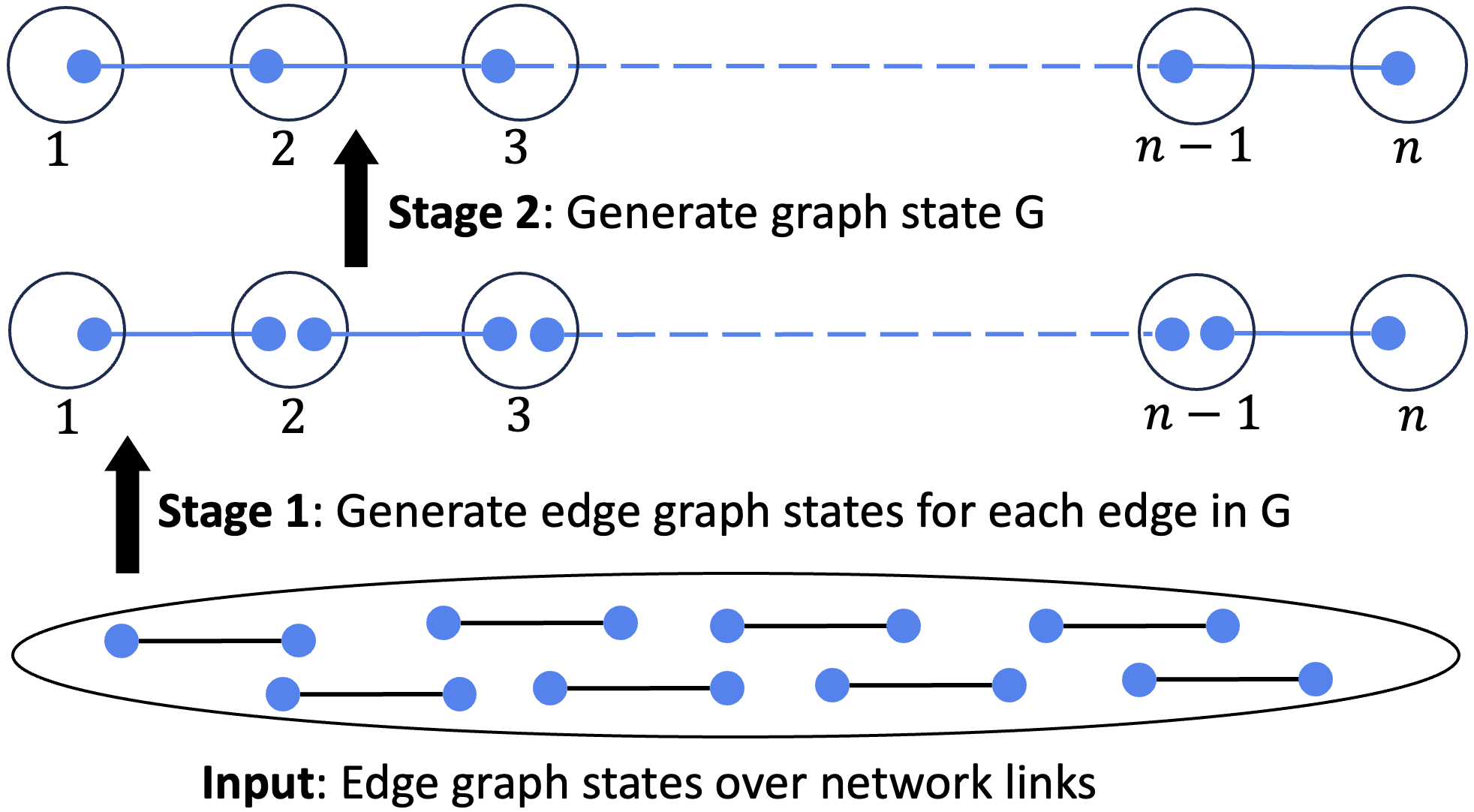
Figure 5: Two-Stage Generation Scheme for a Path Graph State.

Performance Guarantees. We can show the following (we omit the proof).

Theorem 2

The above Two-Stage scheme returns an optimal solution for the special case of the GSG solution mentioned in Theorem 1 with the additional requirement that the level-based structure $L$ has a “barrier” level (i.e., no state at higher level depending on states at lower levels) consisting only of single-edge states corresponding to the edges in $G$.  

VI Generating Tree Graph States

We now design efficient generation schemes to generate tree graph states. Unlike for path graphs, the number of connected induced subgraphs of a tree is exponential in the number of vertices. Thus, considering all connected induced subgraphs (e.g., as in §V-A for paths) is not feasible. In this section, we design two schemes based on a combination of strategies to reduce the number of intermediate states considered.

VI-A Two-Stage Generation Scheme

Consider a GSG problem instance, wherein the target graph state $G$ is a tree $T$. Recall that the target distribution of $G$ over $Q$ is represented by $\tau:V(G)\mapsto V(Q)$.

Basic Idea. As described in previous sections, a Two-Stage approach consists of two stages. In the first stage, we generate single-edge states corresponding to edges in the target state, and then, in the second stage, we iteratively generate appropriate types of intermediate states and, eventually, the target state. Generally, the natural set of intermediate states to consider in the second stage is the set of all connected subgraphs of the target state (as in §V-B for paths). However, for a tree state, that is exponential. Thus, we consider a carefully chosen set of specialized connected subgraphs such that they are polynomial in number, can be computed from link states via other states from this set (in other words, the set of states yields a connected hypergraph), and is “rich” enough to facilitate an efficient LP solution. We start with a notation that defines these specialized subgraphs of trees.

Notation Tree$(p,i\cdotp\cdotp j)$. Consider a GSG problem instance: a quantum network (QN) $Q$ and a tree graph state $T$ along with its target distribution $\tau:V(T)\mapsto V(Q)$. Without loss of generality, we number the children of each non-leaf node $x$ in $T$ from $1$ to $c(x)$, where $c(x)$ is the number of children of $x$ in $T$. Based on such a numbering, the notation Tree$(p,i\cdotp\cdotp j)$, where $p\in V(T)$ and $1\leq i\leq j\leq c(p)$, denotes a distributed tree state $T^{\prime}$ that is an induced subgraph $T^{\prime}$ of $T$ containing the following vertices: (i) node $p$ as $T^{\prime}$ root, (ii) $p$’s $i^{th}$ to $j^{th}$ children along with all their descendants in $T$. In addition, $T^{\prime}$ also uses the same distribution function $\tau$ over its vertices. See Fig. 6.

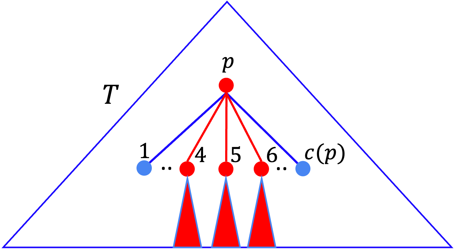
Figure 6: Notation $\texttt{Tree}(p,i\cdotp\cdotp j)$ (here, $i=4,j=6$) denotes a distributed graph state $T^{\prime}$ that is an induced subgraph of $T$ including the interior node $p$, the $i^{th}$ to $j^{th}$ children of $p$ and all their descendants. The graph state $T^{\prime}$ has the same distribution function $\tau()$ as $T$.

Overall Two-Stage Scheme. Our Two-Stage generation scheme for the tree graph states consists of two stages.

• First, from the link states, we generate single-edge graph states corresponding to each edge in $T$. The intermediate states considered in this stage are single-edge distributed graph states for all pairs of network nodes.

• Then, using the above single-edge states (output of the first stage) and other states generated in this second stage, we iteratively generate intermediate states (which include the target state) of the kind $\texttt{Tree}(p,i\cdotp\cdotp j)$ where $p\in V(T)$ and $1\leq i\leq j\leq c(p)$.

For the first stage, we need to use only the fusion-discard operation (see §V-A), while for the second stage, we use the following fusion operations (see Fig. 7).

• $Fusion_{1}$: Fuse Tree$(p,i\cdotp\cdotp j)$ and Tree$(p,{(j+1)}\cdotp\cdotp k)$ to generate Tree$(p,i\cdotp\cdotp k)$.

• $Fusion_{2}$: Fuse Tree$(p,1\cdotp\cdotp c(p))$ and $\langle p,p^{\prime}\rangle$ (with $p$ and $p^{\prime}\in T$ mapped to $\tau(p)$ and $\tau(p^{\prime})$ respectively) to generate Tree$(p^{\prime},i\cdotp\cdotp i)$; here, $p$ is the $i^{th}$ child of $p^{\prime}$ in $T$.

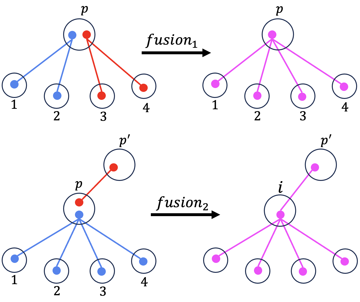
Figure 7: $Fusion_{1}$ and $Fusion_{2}$ operations.

Hypergraph and LP. We now construct a hypergraph with $Avail()$ vertices for all link states and intermediate states (from both stages), and hyperedges to represent the fusion operations over the $Avail()$ vertices as described above. As in the previous section, we add $Prod^{*}$ vertices for each fused $Avail()$ node based on the fusion operation used. We formulate the constraints and the objective function in the LP, as in the previous section. We state the performance guarantee in Theorem 3, in the following subsection.

VI-B One-Stage Generation Scheme

To improve the above Two-Stage LP formulation, we add vertices (and corresponding hyperedges) to the hypergraph of the previous subsection to “bridge the separation” between the two stages. In particular, we expand the previous set of intermediate states by allowing an arbitrary network node to have Tree$(p,i\cdotp\cdotp j)$ as its subtree. The new set of intermediate states is still polynomial in input size, but “connects” the first-stage intermediate states to other stages in the hypergraph of Two-Stage approach and thus enabling a richer set of hyperpaths and level-based structures in the LP.

Notation Tree$(x,p,i\cdotp\cdotp j)$. This denotes a distributed tree graph state $T^{\prime}$ that includes a vertex $x$ (corresponding to an arbitrary network node) as the root, with its sole child as the tree graph state Tree$(p,i\cdotp\cdotp j)$. $T^{\prime}$ distribution function $\tau^{\prime}$ is same as $\tau$ for $p$ and its descendants, and for $x$, $\tau^{\prime}(x)=x$.

Intermediate States, Fusion Operations, Hypergraph. We select the set of intermediate states as all states of the type (i) Tree$(x,p,i\cdotp\cdotp j)$ with $\tau^{\prime}(x)\in V(Q),p\in V(T)$ and $1\leq i\leq j\leq c(p)$, and (ii) Single-edge graph states, for every pair of network nodes; we denote these states by $\langle y,z\rangle$ where $y,z$ are network nodes. We use essentially the similar fusion operation as for the two-stage scheme, except that we also add fusion operations to allow the extension $x$ of $p$ in Tree$(x,p,i\cdotp\cdotp j)$ to extend so that $x$ is mapped to $\tau(p^{\prime})$, at which point, the distributed state transforms to Tree$(\hbox{},p^{\prime},i\cdotp\cdotp i)$. More formally, we allow the following fusion operations:

1. Fusion-discard operation over edge graph states, i.e., fuse states $\langle x,y\rangle$ and $\langle y,z\rangle$ to form $\langle x,z\rangle$.

2. Fuse states Tree$(x,p,i\cdotp\cdotp j)$ and Tree$(\phi,p,{(j+1)}\cdotp\cdotp k)$ to generate Tree$(x,p,i\cdotp\cdotp k)$, and similarly, Tree$(\phi,p,i\cdotp\cdotp j)$ and Tree$(x,p,{(j+1)}\cdotp\cdotp k)$ to generate Tree$(x,p,i\cdotp\cdotp k).$ These are similar to $Fusion_{1}$ in the Two-Stage scheme, but with the $(x,p)$ extension.

3. Fuse states Tree$(x,p,i\cdotp\cdotp j)$ and $\langle y,x\rangle$ to generate Tree$(y,p,i\cdotp\cdotp j)$. This is essentially the fusion-discard operation to extend the extension $(x,p)$.

4. Transform (without any fusion) Tree$(x,p,1\cdotp\cdotp c(p))$ to Tree$(\phi,p^{\prime},i\cdotp\cdotp i)$ where $p$ is the $i^{th}$ child of $p^{\prime}$ in $T$ and $\tau(p^{\prime})=x$.

Based on the above intermediate states and the fusion operations, we construct a hypergraph $H_{1}$ and formulate an LP as before. It is easy to see the following: (i) The hypergraph for the Two-Stage scheme (§VI-A) is an induced subgraph of the above-constructed hypergraph $H_{1}$. (ii) There are level-based structures in $H_{1}$ that do not use any edge graph states corresponding to $T$’s edges—which means that, in this One-Stage scheme, the target graph state $T$ can be potentially generated without going through any edge graph states corresponding to $T$’s edges. (iii) The total number of intermediate states in the above One-Stage scheme is polynomial in the size of the network and the target graph state. We can show the following for both the schemes for tree graph states.

Theorem 3

The Two-State and One-Stage generation schemes above return an optimal solution for the special cases of the GSG problem wherein (a) the target state is a tree graph, (b) the output level-based structure $L$ is such that the vertices and fusion operations used in $L$ are restricted to the intermediate states and fusion operations discussed above, in the respective schemes.  

VII Other Graph States; Multiple Graphs; Fidelity

Generating Other Classes of Graph States. Our LP-based technique for optimized generation of graph states is very versatile; it can be tailored to generate other classes of states.

Grid Graph States. A $(m_{x},m_{y})$-grid graph state $G$ with $m_{x},m_{y}\geq 1$ has a 2D structure consisting of $m_{x}$ columns and $m_{y}$ rows. For such states, it is natural to consider intermediate states of the type $\langle i\cdotp\cdotp j,r\cdotp\cdotp s\rangle$ consisting of $i$ to $j$ rows and $k$ to $l$ columns of $G$; the number of such states is polynomial in the size of $G$. In addition, we must consider $\langle x,y\rangle$ single-edge graph states where $x$ and $y$ are network nodes. To facilitate the generation of $G$ from these intermediate states, we include fusion-retain, fusion-discard, fusion-row and fusion-column operations; Fig. 8 shows the fusion-column operation. With the above intermediate states and fusion operations, we can construct the hypergraph and formulate an LP as before.

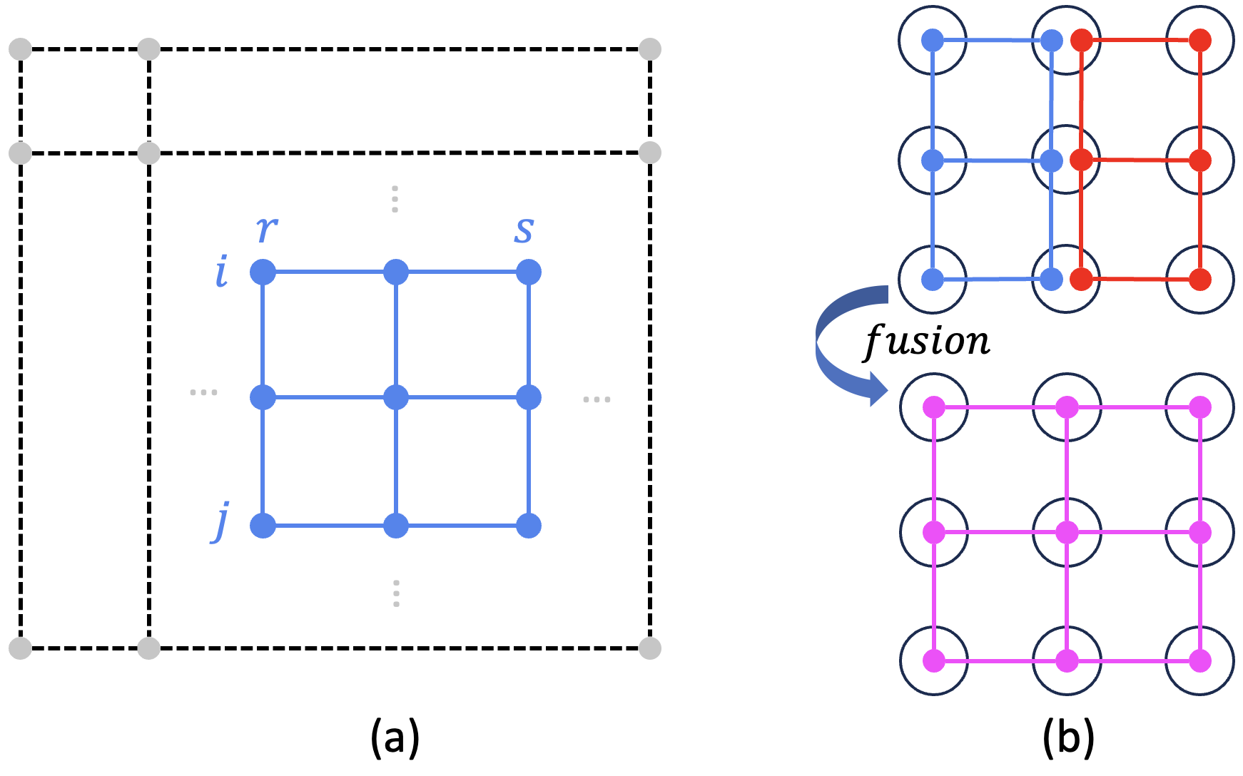
Figure 8: Grid graph states. (a) Intermediate state. (b) Fusion-Grid Operation.

Bipartite Graph States. A $(m_{a},m_{b})$-bipartite graph state $G$ has $m_{a}$ and $m_{b}$ vertices in the two partitions $A$ and $B$ numbered 1 to $m_{a}$ and 1 to $m_{b}$ respectively. To consider a polynomial number of intermediate states, we consider the intermediate states corresponding to the induced subgraphs represented by $\langle i\cdotp\cdotp j,r\cdotp\cdotp s\rangle$ which includes $i$ to $j$-numbered vertices in $A$ and $r$ to $s$-numbered vertices in $B$. See Fig. 9. We include the edge graph states $\langle x,y\rangle$. We can create appropriate fusion operations to generate $\langle i\cdotp\cdotp j,r\cdotp\cdotp s\rangle$ intermediate states; the fusion operations essentially fuse a set of star graphs.

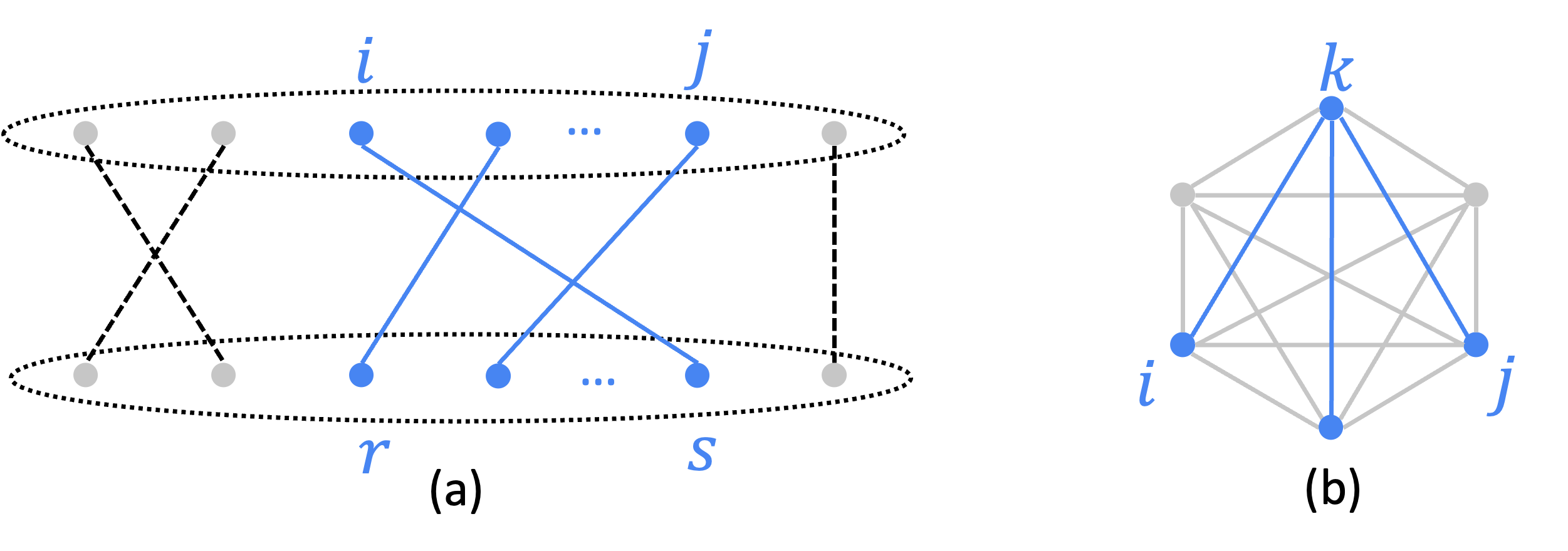
Figure 9: Intermediate states of (a) bipartite graph, (b) complete graph.

Complete or Repeater Graph States. For complete graphs $G$, we can consider the intermediate states as the star graphs $\langle k,i\cdotp\cdotp j\rangle$ with vertex $k$ as its root and vertices numbered $i$ to $j$ (excluding $k$) as its children. Along with the single-edge graph states, the total number of intermediate states is polynomial in the size of $G$, and the only fusion operations needed are fusion-retain, fusion-discard, and a fusion to fuse two star graphs. The above approach easily extends to repeater graphs [16].

Generating Multiple Graph States Concurrently. Our GSG problem considers the generation of (multiple instances of) a single graph state. Our LP formulation can easily be extended to generate several different “types” (including different distributions of the same graph state) of graph states concurrently by essentially creating a hypergraph for each graph state, “merging” the hypergraphs (by taking a union of the vertices and edges, and removing duplicates), and formulating the LP formulation’s objective to maximize the sum (or some linear function) of the generation rates of all the graph states.

Decoherence and Fidelity Constraints. Theoretically, constraints on the loss of fidelity due to noisy fusion operations and the age of qubits can be added to the LP formulation as follows, in a way similar to [17] for swapping trees. First, we observe that the fidelity degradation of a generated graph state due to the number of operations can be modeled by limiting the number of its leaf descendants. Second, as observed in [17] for the case of swapping trees, the decoherence constraint (i.e., bounding the total age of a qubit in a graph state) can be incorporated by limiting the depths of the left-most and right-most descendants of the children of a graph state in the hypergraph. These structural constraints can be enforced in the LP formulation by adding the leaf count and appropriate heights as parameters to $Prod^{*}$ and $Avail^{*}$ vertices.

VIII Evaluations

We now evaluate our schemes and compare them with prior work over the quantum network simulator NetSquid [24].

Graph State Generation Protocol. We build our protocols on top of the link-layer protocol of [25], delegated to continuously generate EPs on a link at a desired rate. The key aspect of our generation protocol is that a fusion operation is done only when both the subgraph states (corresponding to the fusion operands) have been generated. On success of a fusion operation, the fusion node transmits classical information to the terminal nodes of its sub-states to manipulate the gate operations on their qubits. On fusion failure, all the qubits for this graph state will be discarded, allowing the protocols in the lower level to generate new link EPs and subgraphs.

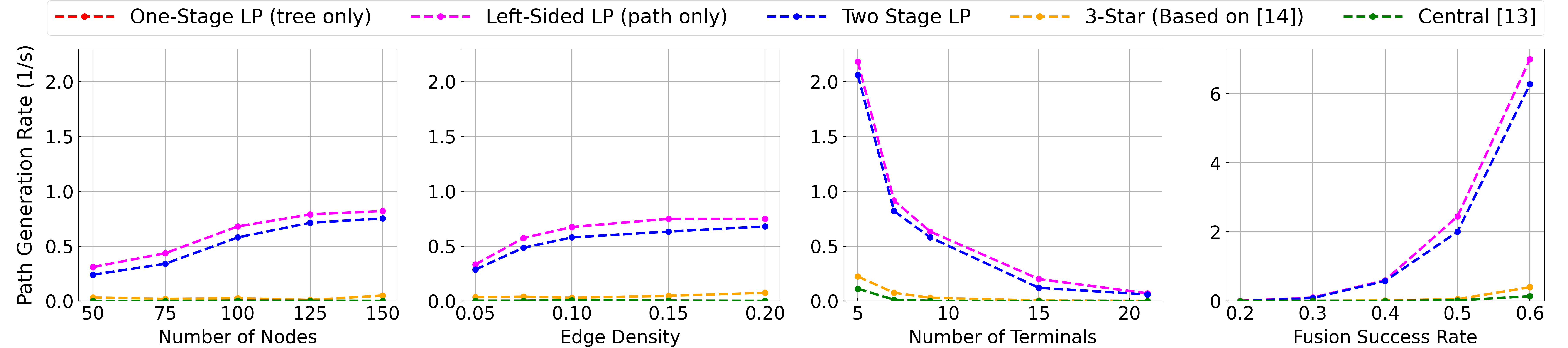
Figure 10: Generation Rates for path graph states for various schemes, for varying parameter values, from NetSquid simulations. (One-Stage takes exorbitant computation time for a 100-node network. Thus, we plot Left-Sided LP scheme; Right-Sided LP scheme has similar performance and not shown.)

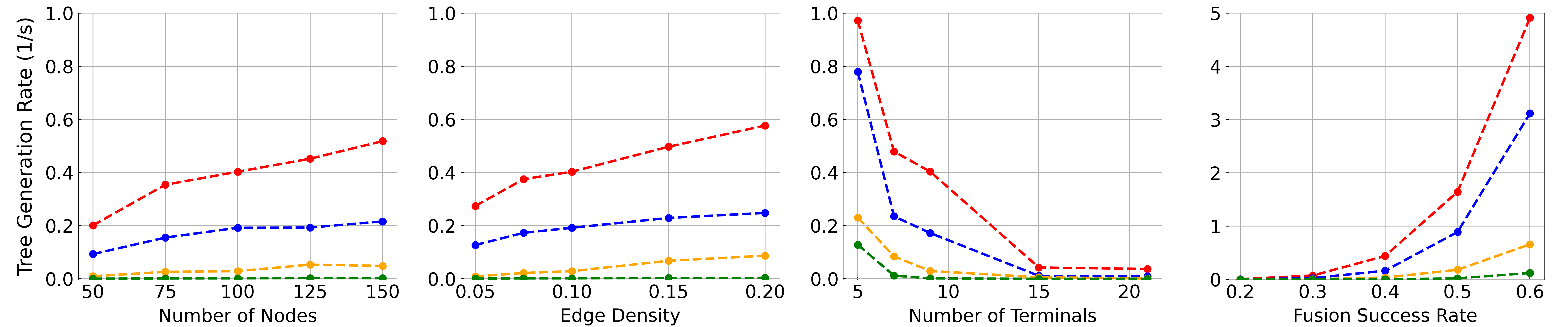
Figure 11: Generation Rates for tree graph states for various schemes, from NetSquid simulations. In (c), for 15-21 terminals, One-Stage has a generation rate of 0.04-0.03, Two-Stage have rates of 0.009-0.0007, while 3-Star and Central have rates of 0.005-0.0005 and $10^{{-}6}$-$10^{{-}8}$ respectively.

Simulation Setting. We generate random quantum networks in a similar way as in the recent works [17, 18]. By default, we use a network spread over an area of $100km\times 100km$. We use the Waxman model [26], used to create Internet topologies, distribute the nodes, and create links. We select the terminal nodes that store the graph state within the network graph, randomly. The path graph state and tree graph state have the same parameter settings. We vary the number of nodes from 50 to 150 (default being 100) and the number of terminals (i.e., size of the graph state) from 5 to 21 (default being 9). The tree state is as follows: root has 2 children, root’s children has 3 children each, and finally, root’s grandchildren have 0-3 children each—yielding a tree of size 9 to 21. We vary the edge density from 0.05 to 0.2 with a default value of 0.1. Each data point is for a 100-second duration simulation in NetSquid.

Parameter Values. We use parameter values similar to the ones used in [20, 17]. In particular, we use fusion probability of success ($p_{f}$) to be 0.4 and latency ($t_{f}$) to be 10 $\mu$ secs; in some plots, we vary $p_{f}$ from 0.2 to 0.6. The atomic-BSM probability of success ($p_{b}$) and latency ($t_{b}$) always equal their fusion counterparts $p_{f}$ and $t_{f}$. The optical-BSM probability of success ($p_{ob}$) is half of $p_{b}$. For generating link-level EPs, we use atom-photon generation times ($t_{g}$) and probability of success ($p_{g}$) as 50 $\mu$sec and 0.33, respectively. Finally, we use photon transmission success probability as $e^{-d/(2L)}$ [20] where $L$ is the channel attenuation length (chosen as 20km for optical fiber) and $d$ is the distance between the nodes. As in [17, 21], we choose a decoherence time of two seconds based on achievable values with single-atom memory platforms [27]; note that decoherence times of even several minutes [28, 29] to hours [30, 31] has been demonstrated for other memory platforms. In NetSquid, we pick the depolarizing channel as our noise model and set the depolarization rate as 0.02.

Prior Algorithms Compared. For comparison with prior work, we implement two schemes: a recent 3-Star-based scheme from [16] (we adapt it for a quantum network) and the flow-based approach (called Central, here) from [15]. We describe these below. The 3-Star approach [16] is a three-step graph-theoretic scheme: simplify the graph state, decompose the simplified graph into star graphs, and replace each star graph into multiple 3-Star states and determine the order of fusion operations; finally, iterate over the above steps and select the best one. To adapt the scheme to generate graph states in a quantum network, we generate the required 3-Star state locally in a central node, distribute (via teleportation) the qubits of the 3-Star states appropriately, and then fuse them to generate the distributed target graph state. The Central approach works by first generating the target graph state locally (at an exhaustively picked optimal central node) and then teleporting the qubits of the graph state to the desired terminals. To continuously generate the graph states at an optimal generation rate, the generation of EPs between $C$ and the terminals is done continuously in parallel with other steps (similar to the max-flow-based approach from [15]).

Our Algorithms. For tree graph states, we implement the One-Stage and Two-Stage schemes. For the path states, the optimal One-Stage scheme (§V-A) takes an exorbitant computation time even for moderate-sized networks; e.g., for a network of 50 (100) nodes, its LP takes 5 (estimated, 120) hours. The Distance-Based approximation schemes perform similarly to One-Stage for $c>0.8$, but also incur very high computation time. In contrast, the Left-Sided and Right-Sided LP schemes take only a few minutes, even for 100-node networks, and perform close to the optimal One-Stage scheme. See Fig. 12. Based on these observations, we only consider Left-Sided and Two-Stage for path graph states for our further evaluations, which are done over large (default 100 nodes) networks; Right-Sided performs similarly to Left-Sided and, thus, is not shown.

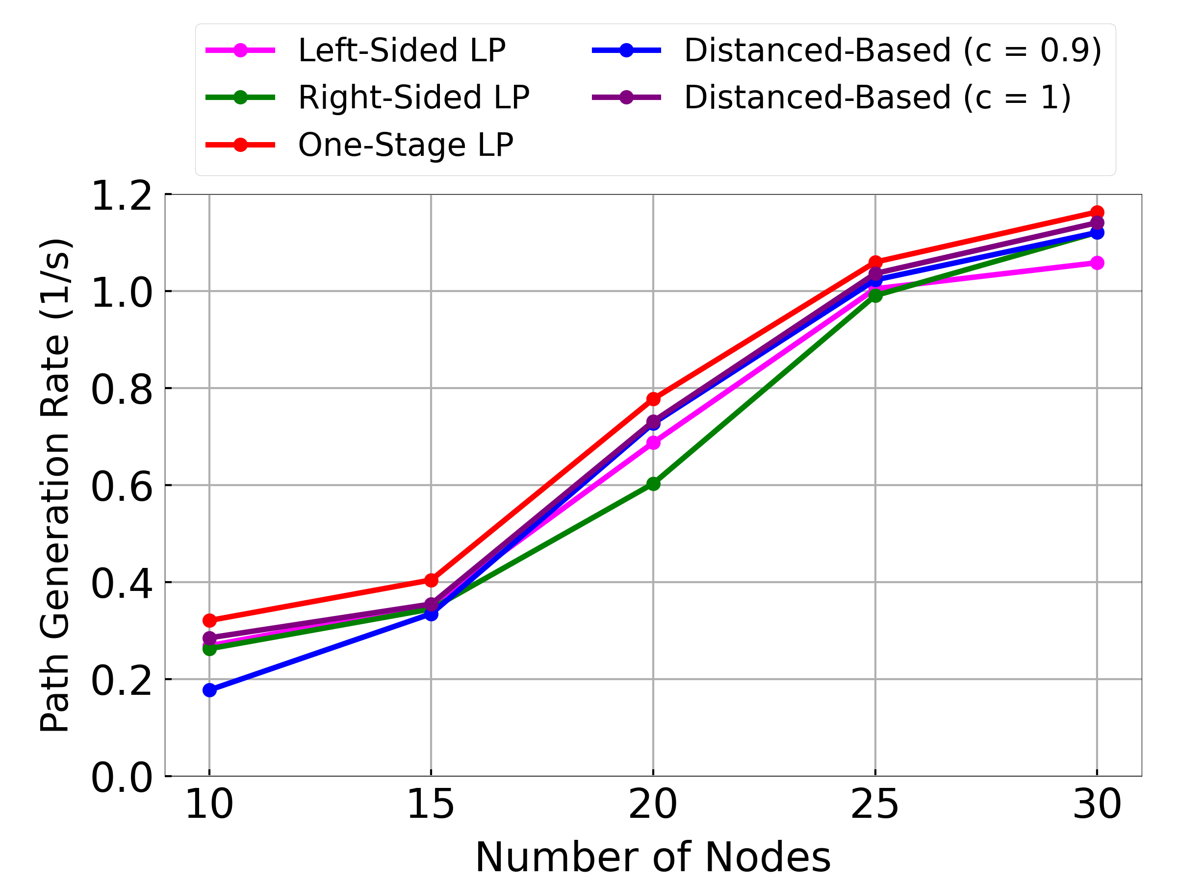
Figure 12: Performance of computationally-efficient approximation schemes for path graph states relative to the optimal One-Stage scheme for small network sizes.

Evaluation Results. We now present the evaluation results comparing prior work with our techniques. Figs.10-11 show the generation rates of various schemes for path and tree graph states, as determined by the NetSquid simulations of at least 100-second duration. In particular, we vary one parameter at a time while keeping the other parameters constant (to their default values). We observe that our schemes outperform the Central and 3-Star schemes for both path and tree graph states by up to orders of magnitude; in particular, the performance gap is about 100 ($\mathbf{10^{6}}$) times wrt 3-Star (Central) for both path and tree graph states of 21 terminals. Among our schemes, as expected, One-Stage outperforms the Two-Stage scheme, sometimes with a smaller margin. Finally, Fig. 13(a)-(b) show the fidelities of the graph states generated in NetSquid simulations by the various schemes for both path and tree graph states for varying fusion success rates. We see that the fidelity of the generated graph states is consistently high. Note that the Central approach has high fidelity since we defer generation of the graph state to after all the EPs required for teleportation have been successfully generated. We observe that generation rates in the NetSquid simulations show a similar trend as those output by the LP solutions (not shown), but the NetSquid simulation rates were consistently higher; this is because the 2/3 factor estimation in Eqn. 1 only holds when the operand generation rates are equal—this holds in the LP solution but may not hold at higher levels of the level-based structure in an actual simulation.

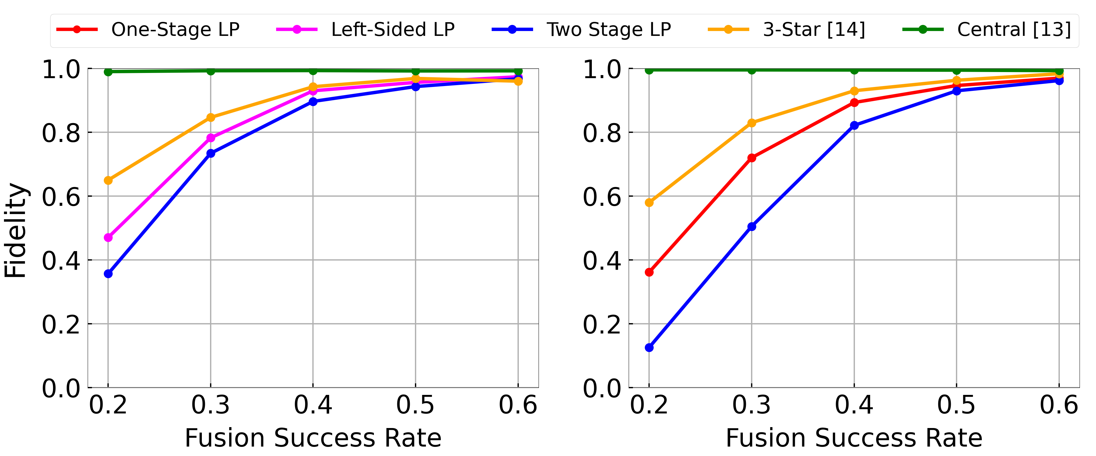
Figure 13: Fidelity of generated graph states. (a) Paths, (b) Trees.

Runtime; Scalability. Our presented schemes take 1-5 minutes to run for 9-terminal states in 100-node networks on a 5GHz machine. This is tolerable overhead for potentially continuous generation of graph states, especially since optimizing generation latency of graph states also minimizes their fidelity degradation due to minimal storage time during generation.

IX Conclusions

We have developed a framework for developing optimized generation and distribution of classes of multipartite graph states under appropriate constraints while considering the stochasticity of the underlying processes. Our future work is focused on developing provably optimal generation schemes under fewer assumptions and/or for other useful classes of graph states.

References

- [1] C. Simon, “Towards a global quantum network,” Nature Photonics, vol. 11, no. 11, pp. 678–680, 2017.
- [2] C. Zhan and H. Gupta, “Quantum sensor network algorithms for transmitter localization,” in IEEE QCE, 2023.
- [3] Z. Eldredge et al., “Optimal and secure measurement protocols for quantum sensor networks,” Physical Review A, 2018.
- [4] V. Scarani et al., “The security of practical quantum key distribution,” Reviews of modern physics, 2009.
- [5] P. Komar, E. M. Kessler, M. Bishof, L. Jiang, A. S. Sørensen, J. Ye, and M. D. Lukin, “A quantum network of clocks,” Nature Physics, 2014.
- [6] T.-Y. Chen et al., “Field test of a practical secure communication network with decoy-state quantum cryptography,” Optics express, 2009.
- [7] M. Marcozzi and L. Mostarda, “Quantum consensus: an overview,” arXiv preprint arXiv:2101.04192, 2021.
- [8] R. G Sundaram, H. Gupta, and C. Ramakrishnan, “Efficient distribution of quantum circuits,” in DISC, 2021.
- [9] C. Zhan, H. Gupta, and M. Hillery, “Optimizing initial state of detector sensors in quantum sensor networks,” ACM TQC, 2024.
- [10] S. Bartolucci, P. Birchall, H. Bombin et al., “Fusion-based quantum computation,” Nature Communications, 2023.
- [11] D. Schlingemann and R. F. Werner, “Quantum error-correcting codes associated with graphs,” Phys. Rev. A, Dec 2001.
- [12] M. Hillery, V. Bužek, and A. Berthiaume, “Quantum secret sharing,” Phys. Rev. A, Mar 1999.
- [13] W. Dür, M. Skotiniotis, F. Fröwis, and B. Kraus, “Improved quantum metrology using quantum error correction,” Phys. Rev. Lett., Feb 2014.
- [14] C. Meignant, D. Markham, and F. Grosshans, “Distributing graph states over arbitrary quantum networks,” Phys. Rev. A, Nov 2019.
- [15] A. Fischer and D. Towsley, “Distributing graph states across quantum networks,” in IEEE QCE, 2021.
- [16] S.-H. Lee and H. Jeong, “Graph-theoretical optimization of fusion-based graph state generation,” Quantum, 2023.
- [17] M. Ghaderibaneh, C. Zhan et al., “Efficient quantum network communication using optimized entanglement swapping trees,” IEEE TQE, 2022.
- [18] S. Shi and C. Qian, “Concurrent entanglement routing for quantum networks: Model and designs,” in SIGCOMM, 2020.
- [19] K. Chakraborty et al., “Entanglement distribution in a quantum network: A multicommodity flow-based approach,” IEEE TQE, 2020.
- [20] M. Caleffi, “Optimal routing for quantum networks,” IEEE Access, 2017.
- [21] M. Ghaderibaneh, H. Gupta, and C. Ramakrishnan, “Generation and distribution of GHZ states in quantum networks,” in IEEE QCE, 2023.
- [22] S. de Bone, R. Ouyang, and K. Goodenough, “Protocols for creating and distilling multipartite GHZ states with bell pairs,” IEEE TQE, 2020.
- [23] L. Bugalho, B. C. Coutinho, and Y. Omar, “Distributing multipartite entanglement over noisy quantum networks,” Quantum, 2021.
- [24] T. Coopmans, R. Knegjens et al., “NetSquid, a discrete-event simulation platform for quantum networks,” Communications Physics, 2021.
- [25] A. Dahlberg, M. Skrzypczyk, T. Coopmans, L. Wubben et al., “A link layer protocol for quantum networks,” in SIGCOMM, 2019.
- [26] B. Waxman, “Routing of multipoint connections,” IEEE Journal on Selected Areas in Communications, 1988.
- [27] P. van Loock et al., “Extending quantum links: Modules for fiber- and memory-based quantum repeaters,” Advanced Quantum Tech., 2020.
- [28] M. Steger, K. Saeedi et al., “Quantum information storage for over 180s using donor spins in a 28si “semiconductor vacuum”,” Science, 2012.
- [29] K. Saeedi, S. Simmons et al., “Room-temperature quantum bit storage exceeding 39 minutes using ionized donors in silicon-28,” Science, 2013.
- [30] M. Zhong, M. P. Hedges, R. L. Ahlefeldt et al., “Optically addressable nuclear spins in a solid with a six-hour coherence time,” Nature, 2015.
- [31] P. Wang, C.-Y. Luan, M. Qiao et al., “Single ion qubit with estimated coherence time exceeding one hour,” Nature communications, 2021.