Context-Aware Mobile Network Performance Prediction Using Network & Remote Sensing Data

Abstract

Accurate estimation of Network Performance is crucial for several tasks in telecom networks. Telecom networks regularly serve a vast number of radio nodes. Each radio node provides services to end-users in the associated coverage areas. The task of predicting Network Performance for telecom networks necessitates considering complex spatio-temporal interactions and incorporating geospatial information where the radio nodes are deployed. Instead of relying on historical data alone, our approach augments network historical performance datasets with satellite imagery data. Our comprehensive experiments, using real-world data collected from multiple different regions of an operational network, show that the model is robust and can generalize across different scenarios. The results indicate that the model, utilizing satellite imagery, performs very well across the tested regions. Additionally, the model demonstrates a robust approach to the cold-start problem, offering a promising alternative for initial performance estimation in newly deployed sites.

I Introduction

Mobile operators across the globe are rolling out the fifth generation (5G) of networks to unlock a wide range of new services and meet high requirements for applications like vehicle-to-vehicle communication. Before rolling out 5G technologies, mobile operators assess the infrastructures and the urban environment to study the feasibility of deploying a new 5G site and upgrading an existing one. Therefore, assisting network planners with a method that predicts network performance while capturing the evolving urban infrastructure is important.

In 5G-and-beyond networks, the process can be even more challenging because of the use of high-frequency bands. High signal frequencies undergo significant attenuation and are distorted while interacting with various objects in the environment. Consequently, it makes it hard to characterize network performance without considering geospatial feature attributes in coverage areas.

Additionally, the number of mobile and IoT devices continues to soar, which forces network operators to work on the dual task of enhancing their existing 4G infrastructure and transitioning to the cutting-edge 5G technologies. One of the primary challenges in this evolution is network densification, characterized by a surge in new cell sites. This transition, though promising in terms of connectivity, brings with it the task of network planning. Network planners need to meticulously determine where to place base stations to optimize both coverage and costs. The dynamics of rapidly growing cities and expanding urban landscapes further complicate this task.

Historically, cellular network planning has been grounded in network data [1], which often overlooks the intricate interplay of various factors influencing network performance. Recognizing this limitation, our research takes another approach; harnessing the power of satellite imagery to estimate Radio Access Network (RAN) performance. By analyzing satellite imagery data, we aim to discern the infrastructure elements and geographical attributes that can impact network performance. Augmenting this information to the historical RAN performance can provide a holistic understanding of network behavior.

It is often said: ”We shape our buildings and afterward our buildings shape us.” Our research is inspired by the idea that spatial structure inherits how end-users use and interact with telecom network. By leveraging satellite imagery, we present an approach to predict network performance in specific areas based on their structural attributes. This method relies on profiling and segmenting geographic regions that share similar underlying dynamics. These satellite images provide a unique perspective on the geographical and environmental factors that can affect network performance, such as topography, urban density, and natural foliage, which in turn influence signal coverage, capacity demands, and service quality. Furthermore, this method not only reduces computational overhead and streamlines processes but also paves the way for building data-driven digital twins for networks [2]. In essence, we are introducing a Remote Sensing-aided approach to predict RAN performance.

The main contributions of this work are four folds:

1. A forecasting model integrating geospatial data from satellite imagery to predict network KPIs effectively.

2. A network profiling method clustering network nodes into groups by geospatial attributes, optimizing computational efficiency.

3. Benchmarking three state-of-the-art computer vision models using the EuroSAT dataset [3].

4. A demonstration of the model’s effectiveness in addressing the cold-start problem, thereby enhancing performance estimations for new and planned network sites.

II Related work

We outline several related works that either inspire the work of predicting Network KPIs or sit more broadly in the space of Remote Sensing for Telecom applications.

Diagnosing network performance is a problem that has historically been studied under various technologies using Network Key Performance Indicators [4]. Machine Learning techniques have been employed to predict network performance. Tran et al. [5] proposed an LSTM model to estimate throughput in 5G and B5G networks. Nabi et al. [6] explore model fusion techniques to combine different deep learning algorithms, namely Long Short-Term Memory (LSTM), Bidirectional LSTM (BiLSTM) and Gated Recurrent Unit (GRU), for better collective performance. Yaqoob et al. [7] developed a GNN-based model to predict network performance by leveraging the spatiotemporal setup of telecom networks, where the network is modeled as a graph structure over which each node maintains a time series. Moreover, KPI prediction has been used for fault detection in mobile network [8] [9] where the predicted performance is compared with real value to detect anomalous data points.

In recent years, there have been a number of papers exploring the interplay between remote sensing and telecom. Thrane et al. [10] presented a model-aided deep learning approach for path loss prediction. In their work, they augmented radio data with rich and unconventional information about the site, e.g. satellite photos, to provide more accurate and flexible models. Similarly, Zhang et al. [11] used top-view geographical images for Radio propagation modeling.

III Data

III-A Key Performance Indicators (KPIs) data

Mobile operators monitor the network continuously to track the behavior of the network using Performance Management (PM) data to gauge network performance. PM data is captured at regular intervals across Radio nodes, in different software and hardware components.

Network performance is assessed using Key Performance Indicators (KPIs) [1]. KPIs are a set of formulas to calculate Performance Indicators using PM [1] and CM [1] data. KPIs are standardized by 3GPP. There exist different categories of KPIs, such as accessibility, mobility, integrity, utilization, and energy performance. The behavior of these KPIs can vary depending on service area characteristics.

KPIs possess a temporal dimension, reflecting the dynamic and evolving nature of network performance over time. This temporal aspect is crucial for understanding patterns, trends, and anomalies in network behavior, as the performance indicators captured at various radio nodes are not static but fluctuate based on numerous factors such as network load, user behavior, and environmental conditions. The temporal variability makes KPIs data a perfect fit for time series analysis techniques to model and predict network performance.
KPIs Data Pre-Processing: PM data was collected over 2 months for different regions of interest, for a total of over 2000 nodes from different cities and regions, using 80% of the data for training, and 20% of the data for testing. PM data is aggregated over 15 minutes. We normalize this data using Min-Max normalization over the 2 months. 24 hours of historical data points are used to forecast the future 8 hours, resulting in a history size of 96 data points and a horizon size of 32 data points.

III-B Cellular coverage areas

Telecom networks consist of a set of interconnected nodes located on physical sites, each cell in a site provides coverage in a geographic area. Each cellular site or antenna is aimed at a specific geographical region. This targeted region or sector can be deduced using a combination of data points like Cell Latitude, Cell Longitude, Cell Azimuth, Antenna Tilt, and Cell Range. We approximate this sector shape as a rectangle, effectively representing each coverage area. A sector area can be estimated as described in this method [12].

III-C Satellite Imagery

Satellite imagery plays a pivotal role in our approach, offering unique insights into the geographical and environmental contexts that influence network performance. Satellites operated by both governmental and private sectors, address numerous needs, such as agriculture, climate monitoring, military reconnaissance, and urban landscape observation. One of the available satellites, the Sentinel satellites series [13] are frequently utilized in commercial and research settings due to their easy accessibility, cost-effectiveness (being open source), and extensive documentation. The Sentinel series offers up to 10-meter spatial resolution for the RGB bands. Thus, for each region of interest, we query satellite imagery and extract the RGB bands to form our images for training the models. Finally, we use the coverage areas defined in III-B to extract the satellite imagery for those coverage areas for each cell in the associated networks. An important note is that we use data from the same season over the regions of interest (Spring), since we assume that weather can affect the network performance.

III-D EuroSAT

EuroSAT dataset [3] provides a diverse collection of images sourced from the Sentinel-2 satellite. With a spectrum spanning 13 bands, the dataset houses 27,000 labeled images, each structured as a 64x64 pixel grid, and belongs to one of ten different classes (Annual Crop, Forest, Herbaceous Vegetation, Highway, Industrial, Pasture, Permanent Crop, Residential, River, Sea and Lake). Each image in the dataset possesses a resolution that ranges between 10m, 20m, and 60m, depending on the specific band.

For our study, we use the RGB bands from the EuroSAT dataset, aligning with the spectral characteristics of the satellite images we gathered for the regions of interest. The EuroSAT images are used to fine-tune the computer vision model to be used later for representation embedding: 70% of the images for training and 30% for testing.

IV Method

IV-A Method Overview

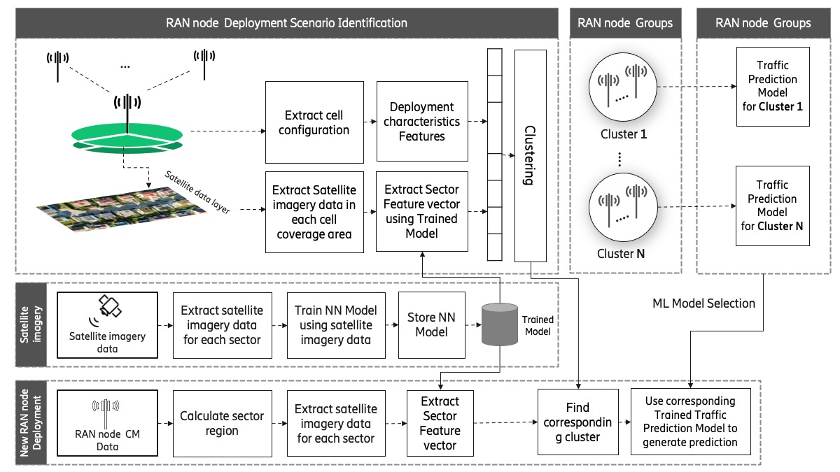
Figure 1: Workflow of the geospatial data-enhanced forecasting methodology. The process begins with the identification of RAN node deployment scenarios, followed by the extraction of cell configuration and satellite imagery data. This data is then utilized to train a neural network model, which informs the clustering of RAN nodes based on deployment characteristics. Each cluster is then associated with a tailored traffic prediction model, allowing for efficient and targeted traffic forecasting across the network.

In this section, we describe our solution. Our method stems from the foundational idea that geospatial attributes of regions, as represented by satellite imagery, can enhance the accuracy and reliability of predicting or forecasting network KPIs. By integrating satellite imagery into our analysis, we harness a deeper layer of contextual information that traditional performance metrics might overlook.

To this end, Figure 1 shows the high level of our proposed solution.

IV-B Vision Models Benchmarking

We adapt and benchmark three state-of-the-art computer vision models on EuroSAT. ResNet-50 [14], EfficientNet [15], and Vision Transformer [16] are trained and evaluated on the EuroSAT dataset train-test splits (70%-30%). Based on evaluation results, the model that exhibits the highest performance on the different metrics (accuracy, precision, recall, and F1-scores) is selected for the next stage of the solution.

IV-C Coverage Areas Satellite Imagery Embedding and Clustering

The selected and trained vision model on EuroSAT is used to generate embedding for the coverage areas for each cellular coverage area and then clustering the embeddings. This is done in 3 steps:

• Step 1: Using the bounding box coordinates (latitude and longitude) calculated for each coverage area, the satellite image is extracted for that node.

• Step 2: The extracted satellite image is passed through the vision model, and the embeddings are extracted from the penultimate layer of the network.

• Step 3: The set of embeddings for all the cellular coverage areas are clustered using KMeans and Elbow method to determine the optimal number of clusters. This results in a set of clusters of nodes whose coverage areas share similar embeddings, i.e., similar geographical infrastructure as identified by the satellite images. Note that EuroSAT was only used for generating embeddings for the satellite coverage areas.

IV-D KPI Forecasting

We utilize LSTM (Long Short-Term Memory) model to forecast the KPIs, with 24 hours of history to forecast the future 8 hours and a moving window of 15 minutes at a time. Two experiments are performed:

1. One LSTM forecasting model trained on the average distribution of the KPIs per cluster and then evaluated.

2. Cold-start analysis: cold-start is a common problem in machine learning, where historical data is not present for future analysis and forecasting. In the context of our work, we employ transfer learning per cluster, where we mask 20% of the nodes per cluster and assume there is no historical data for them, train on 80% of the nodes of that cluster, and evaluate the resulting model on the masked nodes. This way, we are tackling the cold-start problem by assigning nodes with no historical data to clusters whose nodes have similar coverage areas as identified by the satellite imagery embeddings.

IV-E End-to-End Steps

To encapsulate the entire process, we illustrate the proposed end-to-end steps in one flow diagram. The steps can be seen in Figure 2. For network planning, all that is needed is a satellite image of the coverage area intended the site or cell to be deployed. In steps 1 and 2, the vision model is used to extract vector embeddings for the coverage area. Then this embedding gets assigned to a particular cluster of the existing clusters in the network. Using the historical data and model trained on the average distribution of the cluster KPI data, future KPI can be forecasted for the node intended to be deployed in that region identified by the satellite image.

Figure 2: Diagram illustrating the proposed end-to-end pipeline steps KPI prediction using satellite imagery.

V Experiments and Results

V-A Vision Models Results

Table I summarizes the performance metrics of the three models on the test set of EuroSAT. The evaluation of model performance reveals closely matched metrics, with EfficientNet-B0 and ViT slightly outperforming ResNet-50 in terms of accuracy. Based on these findings, EfficientNet-B0 is selected for generating embeddings for the satellite images, thanks to its superior balance of accuracy and efficiency, as well as a relatively lower number of parameters compared to ViT.

TABLE I: Model Performances on EuroSAT Dataset

Model	Accuracy	Precision	Recall	F1 Score	Parameters
ResNet50	0.83	0.86	0.83	0.82	25,557,032
EfficientNet-B0	0.88	0.88	0.87	0.88	5,288,548
Vision Transformer (ViT)	0.88	0.88	0.88	0.88	86,567,656

The penultimate layer of EfficientNet-B0, chosen for embedding extraction, features a dimensionality conducive to representing the complex features of satellite imagery. Embedding vectors for each satellite image within any coverage area will therefore be derived from this layer, offering a sizeable yet efficient 1280-dimensional representation for each image.

V-B Coverage Area Embeddings and Clustering

EfficientNet is used to generate embeddings for each cellular coverage area in our dataset. Using KMeans and the ELbow curve, we cluster the nodes into 35 groups. This is visualized in Figure 3.

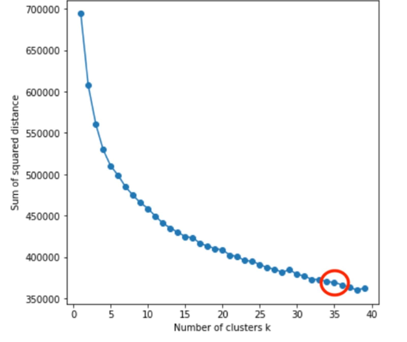
Figure 3: Elbow method visualization for determining the optimal number of clusters in K-means clustering. The curve shows a distinct bend at the point circled in red, indicating that 35 clusters result in a reasonable trade-off between within-cluster variance and the number of clusters.

V-C KPI Predictions

Two experiments are done for KPI prediction:

1. LSTM model trained on average distribution of cells KPI data per cluster and evaluated on individual cells per corresponding cluster.

2. Cold-Start Problem: LSTM model trained on average distribution of 80% of cells per cluster and evaluated on the rest 20% masked cells (without historical data).

Figure 4 provides a visual example that demonstrates robust performance of the proposed model for experiment 1 over a multi-day period in the test set. The overlaid lines of actual and predicted traffic volumes provide clear evidence that the model captures the essential trends and fluctuations in the data.

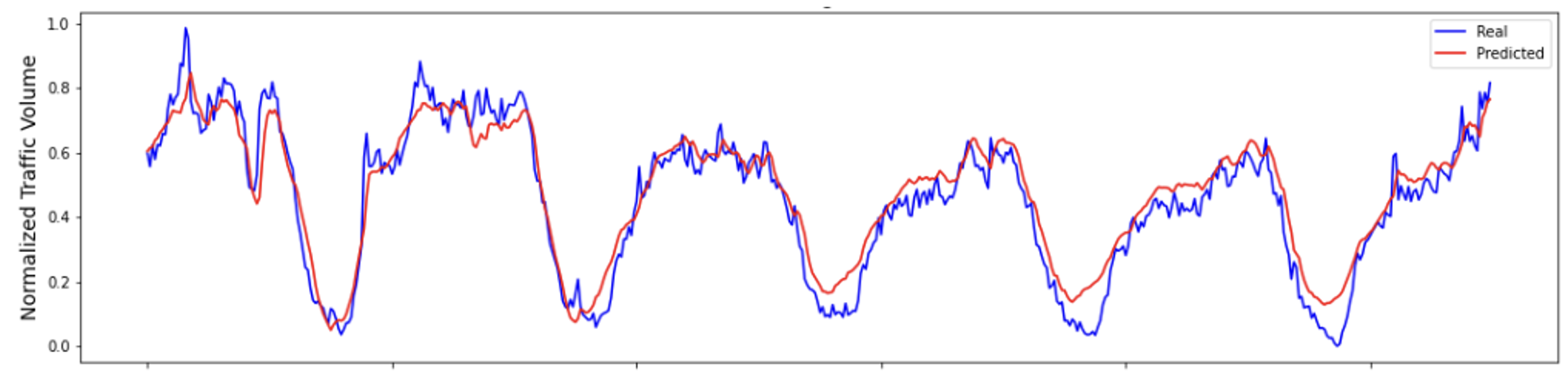
Figure 4: Comparison of real vs. predicted normalized traffic volume. The plot illustrates the close alignment between the actual data (blue) and the predictions (red) from the model, demonstrating how the average model can be used to forecast traffic for individual nodes per cluster.

The numerical results can be found in table II. The metrics shown are the average over all the cells metrics per cluster. For a more detailed analysis and visual comparison, Figure 5 shows the error plot of each metric (MSE and MAE) over all the different nodes in a cluster. The figure indicates that the cold-start results are comparable with training a model on the average distribution per cluster. This indicates that our method is scalable for new sites that are introduced to the network, using assignment procedures from satellite imagery embeddings.

TABLE II: Forecasting Performance Metric Averages

Metric	Experiment 1:	Experiment 2:
	Model per Cluster	Cold-Start Transfer Learning
MSE	$0.0091\pm 0.0024$	$0.0085\pm 0.0034$
MAE	$0.0591\pm 0.0087$	$0.0580\pm 0.0105$

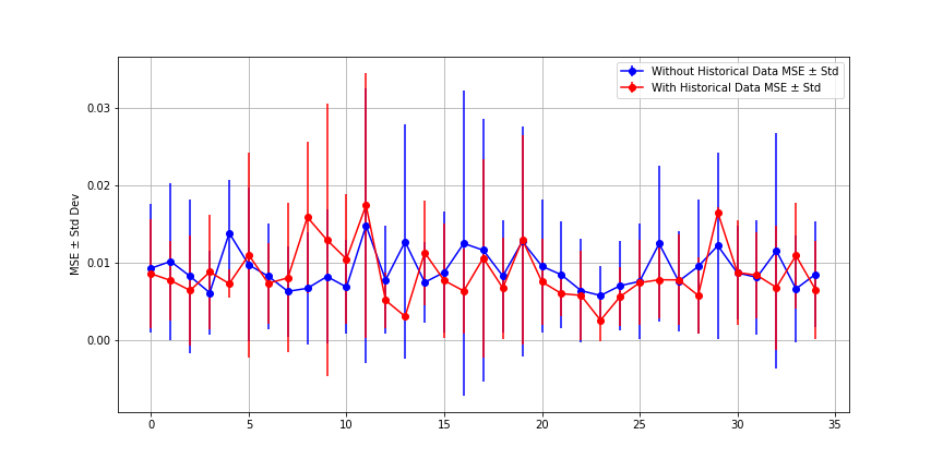
(a) MSE comparison

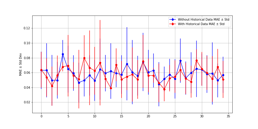
(b) MAE comparison

Figure 5: Comparison of MSE and MAE with Standard Deviation per Cluster for Cold Start vs Non-Cold Start scenarios. Note how cold-start values are comparable with the values with historical data.

VI Discussion

VI-A Reflecting on the Vision Model Results

The performance of the vision models on the EuroSAT dataset was comparable. EfficientNet-B0 and ViT have demonstrated a slight edge in accuracy over ResNet-50. This marginal yet notable superiority underlines the effectiveness of scaling model depth and width, and attention mechanisms in capturing complex spatial hierarchies. Furthermore, EfficientNet-B0 has the least number of parameters as compared to ViT and ResNet50, yet it scored comparably high performance. This emphasizes that model size is not the most important factor for all problems.

The clustering performed on the vision embeddings extracted from EfficientNet-B0 has unveiled a heterogeneous distribution of nodes among the clusters. Some clusters are densely populated, signifying areas with high feature similarity among the images. In contrast, other clusters contain fewer nodes, which may point to more unique, less frequently occurring features within the dataset.

This disparity in cluster sizes is indicative of the diverse nature of land use and cover as captured by satellite imagery. Clusters with a higher number of nodes might represent common or generic features across different regions, such as widespread agricultural areas or urban settings. On the other hand, clusters with fewer nodes could correspond to unique or specific features that are less common or have higher variability, such as rare vegetation types or particular infrastructural elements.

VI-B Reflecting on the forecasting results

The implementation of the LSTM forecasting model, tailored to average distributions per cluster, showcases important results in our study. Particularly, the application of this model on test datasets revealed low MSE and MAE values, underscoring the model’s robust predictive accuracy. This success extends to the cold-start problem, where the performance of the model on clusters without historical data was comparable to those with rich historical records. Such findings illustrate the method’s versatility and its capacity to generate reliable forecasts when based on satellite imagery data.

A significant contribution as well is the computational efficiency achieved through the clustering approach. Traditionally, forecasting models in network systems tend to adopt a one-model-per-cell strategy, leading to extensive computational demands as the number of cells (N) increases. Our method, however, consolidates this approach into a single model per cluster of cells, transitioning the computational complexity from O(N) to O(1). This reduction not only signifies efficient computational resource management but also scalability, enabling the deployment of forecasting models in much larger network systems without the linear increase in computational burden, relying purely on the geo-spatial attributes of the region of interest identified by satellite imagery.

VI-C Reflection on Satellite Imagery

Furthermore, this study introduces the proposition of integrating satellite imagery as a pivotal component in forecasting Network KPIs. The utilization of such imagery extends the forecasting capabilities beyond conventional traffic KPIs, incorporating a spatial dimension that offers a more nuanced understanding of the factors influencing network performance. This approach opens the door to exploring a broader array of geospatial factors, including but not limited to, urban development, environmental changes, and socio-economic activities, all of which can influence network demand and performance. By acknowledging the importance of satellite imagery and geospatial data, we advocate for a more holistic approach to forecasting that leverages the richness of spatial data to enhance prediction accuracy and operational efficiency in networked systems.

VII Conclusion

In this study, we’ve demonstrated that forecasting network traffic with the integration of geospatial data, particularly through satellite imagery, yields positive results and good performance. The strategic use of clustering based on geospatial attributes has substantially reduced computational demands, enabling a deeper understanding of network infrastructure and the geographical context of different sites. Notably, this approach has proven effective for newly deployed or sites planned to be deployed, addressing the cold-start problem with high-performance levels comparable to established sites. By leveraging clusters informed by geospatial data, our model offers a scalable solution for network forecasting that also sets a promising foundation for further research in utilizing geospatial data for KPI forecasting. This approach not only enhances current forecasting methods but also opens the door to innovative strategies in network management and planning. Future research could explore the integration of real-time geospatial data for more accurate and responsive forecasting, and the application of advanced analytics to optimize network deployment in rapidly changing environments. Such studies would further our understanding of how geospatial insights can be leveraged to improve network performance and planning.

References

- [1] 3GPP, “The 3rd generation partnership project,” tech. rep., 2023.
- [2] L. U. Khan, Z. Han, W. Saad, E. Hossain, M. Guizani, and C. S. Hong, “Digital twin of wireless systems: Overview, taxonomy, challenges, and opportunities,” IEEE Communications Surveys & Tutorials, 2022.
- [3] P. Helber, B. Bischke, A. Dengel, and D. Borth, “Eurosat: A novel dataset and deep learning benchmark for land use and land cover classification,” 2019.
- [4] A. Mourad, R. Yang, P. H. Lehne, and A. De La Oliva, “Towards 6g: Evolution of key performance indicators and technology trends,” in 2020 2nd 6G wireless summit (6G SUMMIT), pp. 1–5, IEEE, 2020.
- [5] N. P. Tran, O. Delgado, B. Jaumard, and F. Bishay, “Ml kpi prediction in 5g and b5g networks,” in 2023 Joint European Conference on Networks and Communications & 6G Summit (EuCNC/6G Summit), pp. 502–507, IEEE, 2023.
- [6] S. T. Nabi, M. R. Islam, M. G. R. Alam, M. M. Hassan, S. A. AlQahtani, G. Aloi, and G. Fortino, “Deep learning based fusion model for multivariate lte traffic forecasting and optimized radio parameter estimation,” IEEE Access, vol. 11, pp. 14533–14549, 2023.
- [7] M. Yaqoob, R. Trestian, and H. X. Nguyen, “Data-driven network performance prediction for b5g networks: a graph neural network approach,” in 2022 IEEE Ninth International Conference on Communications and Electronics (ICCE), IEEE, 2022.
- [8] T. Zanouda, S. Govindaraj, D. Budyn, and M. Rydar, “Methods and apparatuses for detecting and localizing faults using machine learning models,” 2022. PCT/EP2022/071544.
- [9] R. Bourgerie and T. Zanouda, “Fault detection in telecom networks using bi-level federated graph neural networks,” in 2023 IEEE International Conference on Data Mining Workshops (ICDMW), pp. 1608–1617, 2023.
- [10] J. Thrane, B. Sliwa, C. Wietfeld, and H. L. Christiansen, “Deep learning-based signal strength prediction using geographical images and expert knowledge,” in GLOBECOM 2020-2020 IEEE Global Communications Conference, pp. 1–6, IEEE, 2020.
- [11] X. Zhang, X. Shu, B. Zhang, J. Ren, L. Zhou, and X. Chen, “Cellular network radio propagation modeling with deep convolutional neural networks,” in Proceedings of the 26th ACM SIGKDD International Conference on knowledge discovery & data mining, pp. 2378–2386, 2020.
- [12] T. Zanouda, “Methods and nodes for predicting azimuth values of cells in communications networks,” 2022. PCT/EP2022/072279.
- [13] E. S. Agency, “Sentinel-2,” 2015. Accessed on February 2, 2024.
- [14] K. He, X. Zhang, S. Ren, and J. Sun, “Deep residual learning for image recognition,” 2015.
- [15] M. Tan and Q. V. Le, “Efficientnet: Rethinking model scaling for convolutional neural networks,” 2020.
- [16] A. Dosovitskiy, L. Beyer, A. Kolesnikov, D. Weissenborn, X. Zhai, T. Unterthiner, M. Dehghani, M. Minderer, G. Heigold, S. Gelly, J. Uszkoreit, and N. Houlsby, “An image is worth 16x16 words: Transformers for image recognition at scale,” 2021.