On the volume of convolution bodies in the plane

Abstract.

For every convex body $K\subset\mathbb{R}^{n}$ and $\delta\in(0,1)$, the $\delta$-convolution body of $K$ is the set of $x\in\mathbb{R}^{n}$ for which ${\left|K\cap(K+x)\right|}_{n}\geq\delta{\left|K\right|}_{n}$. We show that for $n=2$ and any $\delta\in(0,1)$, ellipsoids do not maximize the volume of the $\delta$-convolution body of $K$, when $K$ runs over all convex bodies of a fixed volume. This behavior is somehow unexpected and contradicts the limit case $\delta\to 1^{-}$, which is governed by the Petty projection inequality.

1. Introduction

Let $K\subseteq\mathbb{R}^{n}$ be a convex body (compact, convex and with non-empty interior) and let $g_{K}(x)={\left|K\cap(K+x)\right|}_{n}$ denote the covariogram function, where ${\left|\ \cdot\ \right|}_{n}$ is the $n$-dimensional Lebesgue measure. For $\delta\in(0,1)$, the convolution body of parameter $\delta$ is the set defined by

$$C_{\delta}K=\{x\in\mathbb{R}^{n}:g_{K}(x)\geq\delta{\left|K\right|}_{n}\}.$$

The set $C_{\delta}K$ is called the convolution body of $K$, due to the fact that $g_{K}$ is the convolution of the indicator functions of $K$ and $-K$. Convolution bodies and the covariogram function were studied in [8, 9, 10, 12, 14]. Specifically, in relation to the phase retrieval problem in Fourier analysis, it was studied in [1, 2, 3].

When $\delta\to 1^{-}$ the set $C_{\delta}K$ collapses to the origin. The shape of $C_{\delta}K$, if scaled by a factor $(1-\delta)^{-1}$, approaches the polar projection body of $K$ denoted by $\Pi^{*}K$, which is the unit ball of the norm defined by

$$\|v\|_{\Pi^{*}K}={\left|P_{v^{\perp}}K\right|}_{n-1}$$

for every unit vector $v\in S^{n-1}$, where $P_{v^{\perp}}$ is the orthogonal projection to the hyperplane orthogonal to $v$. This was first observed by Matheron in [9], where the covariogram function was introduced. Indeed it was proven in [12, Theorem 2.2] that

(1) $$\lim_{\delta\to 1^{-}}\frac{{\left|C_{\delta}K\right|}_{n}}{(1-\delta)^{n}}={{\left|\Pi^{*}K\right|}_{n}}.$$

The classical Petty projection inequality (see Section 10.9 of [13]) states that

(2) $${\left|\Pi^{*}K\right|}_{n}\leq{\left|\Pi^{*}B_{K}\right|}_{n}$$

where $B_{K}$ is the Euclidean ball with same volume as $K$. Equality holds in (2) if and only if $K$ is an ellipsoid (an affine image of the Euclidean ball). The left-hand side of inequality (2) is invariant under volume-preserving affine transformations. This was proven by Petty in [11], and Schmuckenschläger gave a simpler proof of this fact using (1) and the obvious fact that $C_{\delta}\varphi(K)=\varphi(C_{\delta}K)$ for every volume-preserving affine transformation $\varphi$.

In the opposite endpoint, $\delta\to 0^{+}$, the body $C_{\delta}K$ converges to the difference body of $K$, defined by

$$DK=\{x-y:x,y\in K\}.$$

By the Brunn-Minkowsky inequality (see [13, Theorem 7.1.1]), ${\left|DK\right|}_{n}\geq 2^{n}{\left|K\right|}_{n}$, with equality if and only if $K$ is symmetric with respect to some point (i.e. $x_{0}+K=x_{0}-K$ for some $x_{0}\in K$). Since $B_{K}$ is origin-symmetric,

(3) $${\left|DK\right|}_{n}\geq{\left|DB_{K}\right|}_{n},$$

which is reverse to the inequality (2). Nevertheless, (3) is an equality for all symmetric sets.

An extension of the Petty projection inequality to certain averages of volumes of $C_{\delta}K$ can be deduced from the results in [8].

Theorem 1.1.

For every non-decreasing function $\omega:[0,1]\to[0,\infty)$ and every convex body $K$,

$$\int_{0}^{1}\omega(\delta){\left|C_{\delta}K\right|}_{n}d\delta\leq\int_{0}^{1}\omega(\delta){\left|C_{\delta}B_{K}\right|}_{n}d\delta.$$

The results in [8] follow from the well-known Riesz convolution inequality, and Theorem 1.1 recovers the Petty projection inequality (without the equality case) thanks to (1) and a limit argument. Namely, one chooses $\omega$ to be an approximation of the Dirac delta at $1$. Since $\omega$ must be non-decreasing, this argument cannot be applied to a Dirac delta at some other point in $(0,1)$. A particular case of Theorem 1.1 is that

$$\int_{t}^{1}{\left|C_{\delta}K\right|}_{n}d\delta\leq\int_{t}^{1}{\left|C_{\delta}B_{K}\right|}_{n}d\delta$$

for any $t\in(0,1)$.

A second application of the Riesz convolution inequality to convex bodies defined from $C_{\delta}K$, was given in [6].

A radial set is a set of the form

$$K=\{0\}\cup\{x\in\mathbb{R}^{n}\setminus\{0\}:|x|\leq\rho_{K}(x/|x|)\}$$

where $\rho_{K}:S^{n-1}\to(0,\infty)$ is continuous, and $|\,\cdot\,|$ is the Euclidean norm. A radial body is a radial set for which $\rho_{K}$ is strictly positive. Every convex body is also a radial body.

For every convex body $K$ and $p>-1,p\neq 0$, the $p$-radial mean body of $K$ is the radial body defined by

$$\rho_{R_{p}K}(v)=\left(\int_{0}^{1}\rho_{C_{\delta}K}(v)^{p}d\delta\right)^{1/p},$$

while $R_{0}K$ is defined as a limit of the sets $R_{p}K$ when $p\to 0$. The original definition given in [5] is different, but equivalent to ours. This can be deduced easily from formulas (3), (16) and (17) in [7].

Theorem 1.2 ( [6, Theorem 20]).

For every convex body $K$ and $p\in(-1,n)$,

$${\left|R_{p}K\right|}_{n}\leq{\left|R_{p}B_{K}\right|}_{n}.$$

For $p>n$ the inequality is reversed. Equality holds if and only if $K$ is an ellipsoid.

It was proven in [5] that $R_{p}K$ approaches $\Pi^{*}K$ when $p\to-1^{+}$, so Theorem 1.2 is yet an other extension of the Petty projection inequality involving averages of $C_{\delta}K$.

Theorems 1.1 and 1.2 suggest the possibility that for a fixed $\delta\in(0,1)$, ${\left|C_{\delta}K\right|}_{n}$ is also maximized by ellipsoids, among sets of a fixed volume. Of course, due to (3) this is only possible if we restrict the problem to the symmetric case, or to some range of $\delta\in(0,1)$ far from $0$. Let us formulate the weakest possible question:

Question 1.3.

Is there a value of $\delta\in(0,1)$ such that

(4) $${\left|C_{\delta}K\right|}_{n}\leq{\left|C_{\delta}B_{K}\right|}_{n}$$

for every symmetric convex body $K$?

The purpose of this paper is to give a complete answer to this question in dimension $2$.

Observe that due to Theorem 1.1, inequality (4) holds “in average” in $\delta$ for every $K$.

The following proposition describes the situation in which $K$ is far from the set of ellipsoids. Define the Banach-Mazur distance between two convex bodies $K,L\subseteq\mathbb{R}^{n}$ as

$$d_{\operatorname{BM}}(K,L)=\min\{\lambda>0:K-x\subseteq\Phi(L-y)\subseteq e^{\lambda}(K-x)\text{ for }\Phi\in GL(n),x,y\in\mathbb{R}^{n}\}.$$

where $GL(n)$ is the set of invertible linear transformations of $\mathbb{R}^{n}$. Let $\mathbb{B}$ be the unit Euclidean ball in $\mathbb{R}^{n}$. It follows from the definition that $d_{BM}(K,\mathbb{B})=0$ if and only if $K$ is an ellipsoid.

Proposition 1.4.

For every convex body $K\subseteq\mathbb{R}^{n}$ which is not an ellipsoid, ${\left|C_{\delta}K\right|}_{n}\leq{\left|C_{\delta}B_{K}\right|}_{n}$ for every $\delta>\varphi(d_{BM}(K,\mathbb{B}))$, where $\varphi:[0,\infty)\to(0,1]$ is a continuous function with $\varphi(t)=1$ if and only if $t=0$.

We will prove this fact in Section 4. Proposition 1.4 reduces the problem to a local question: If (4) is valid for every $K$ sufficiently close to the Euclidean ball and $\delta$ close to $1$, then thanks to Proposition 1.4, it is valid for every $K$ and $\delta$ close to $1$.

Definition 1.5.

For any radial set $K$ we will consider a one-parameter family of radial bodies $K_{t}$ defined by

(5) $$\rho_{K_{t}}(v)=1+t\rho_{K}(v).$$

We also define

(6) $$\overline{K_{t}}=K_{t}/{\left|K_{t}\right|}_{n}^{1/n}.$$

We will say that a radial set $K$ is $C^{\beta}$ smooth with $\beta\geq 1$ if the radial function $\rho_{K}$ is $C^{\beta}$. Notice that this definition does not coincide with the smoothness of the set $\partial K$ as usual, because we are allowing $\rho_{K}(v)=0$. But it is clear that if $K$ is $C^{\beta}$ smooth, then $K_{t}$ has a smooth boundary in the usual sense.

We will analyze ${\left|C_{\delta}\overline{K_{t}}\right|}_{n}$ as a function of $t$ and $\delta$, for $t$ near $0$. First we obtain:

Theorem 1.6.

For every $C^{1}$ radial set $K\subseteq\mathbb{R}^{n}$ and $\delta\in(0,1)$, the function $t\mapsto{\left|C_{\delta}\overline{K_{t}}\right|}_{n}$ is $C^{1}$ and we have

$$\frac{\partial}{\partial t}{\left|C_{\delta}\overline{K_{t}}\right|}_{n}\bigg{|}_{t=0}=0.$$

Then it suffices to analyze the second derivative of $t\mapsto{\left|C_{\delta}\overline{K_{t}}\right|}_{n}$. In the limit $\delta\to 1^{-}$ this second derivative is completely described in Section 6 for $n=2$, and its sign is compatible with the fact that $t\mapsto{\left|\Pi^{*}\overline{K_{t}}\right|}_{n}$ has a maximum at $t=0$. In Section 6 we show:

Theorem 1.7.

For every $C^{2}$ smooth radial set $K\subseteq\mathbb{R}^{2}$ the function $t\mapsto{\left|C_{\delta}\overline{K_{t}}\right|}_{n}$ is $C^{2}$ for every $\delta\in(0,1)$ and

(7) $$\lim_{\delta\to 1^{-}}\frac{1}{(1-\delta)^{2}}\frac{\partial^{2}}{\partial t^{2}}{\left|C_{\delta}\overline{K_{t}}\right|}_{2}\bigg{|}_{t=0} \leq 0.$$

Equality holds if and only if $\rho_{K}$ is the restriction of a homogeneous polynomial of degree $2$ to the unit circle.

The equality cases of Theorem 1.7 correspond to variations $\overline{K_{t}}$ that coincide up to first order with families of ellipsoids.

At this point it is natural to expect that Theorem 1.7 combined with an approximation argument and Proposition 1.4, could yield a positive answer to Question 1.3. However, for this argument to be complete we need the convergence of the second derivatives of the volume as $\delta\to 1^{-}$, to be uniform with respect to $K$. We were unable to show this uniform convergence, and the following counterexample shows why:

Theorem 1.8.

Let $K^{m}\subseteq\mathbb{R}^{2}$ be the (symmetric) radial set defined by $\rho_{K^{m}}(v)=\cos(2mv)^{2}$ with $v\in[0,2\pi]$. Then for every $\delta\in(0,1)$ there exists $m\in\mathbb{N}$ such that

$$\frac{\partial^{2}}{\partial t^{2}}{\left|C_{\delta}\overline{K_{t}^{m}}\right|}_{2}\bigg{|}_{t=0}>0.$$

As a consequence, we get a negative answer to Question 1.3 in dimension $2$, and every value of $\delta\in(0,1)$.

Theorem 1.9.

For every $\delta\in(0,1)$ there exists a symmetric convex body $K\subseteq\mathbb{R}^{2}$ such that ${\left|C_{\delta}K\right|}_{n}>{\left|C_{\delta}B_{K}\right|}_{n}$. Moreover, $K$ can be chosen arbitrarily close to the Euclidean ball in the $C^{\infty}$ topology.

It is important to remark that for a fixed $m$ in Theorem 1.8, the set of $\delta\in(0,1)$ for which $\frac{\partial^{2}}{\partial t^{2}}{\left|C_{\delta}\overline{K_{t}}\right|}_{2}\bigg{|}_{t=0}$ is positive, is a complicated union of intervals that grow in number and accumulate near $1$, as $m\to\infty$. Previous attempts to find regular polygons being counterexamples to Question 1.3 for $\delta$ close to $1$ by direct computation, failed probably because of this complicated behaviour. We still do not know if regular polygons are counterexamples to Question 1.3.

The following natural question remains open:

Question 1.10.

For each fixed $\delta\in(0,1)$, what convex bodies are maximizers of $C_{\delta}K$ when $K$ runs among sets of the same volume?

The rest of the paper is organized as follows:

In Section 2 we introduce al the notation that will be necessary for our computations in the following sections. In Section 3 we obtain the results concerning convex sets far from the ball (Proposition 1.4), and establish several technical lemmas that will be needed later.

In Section 4 we compute the first-order approximation of ${\left|C_{\delta}\overline{K_{t}}\right|}_{n}$ at $t=0$ (Theorem 1.6). All results in this section are stated in $\mathbb{R}^{n}$.

In Section 5 we compute the second order approximation in the plane, and establish Theorems 1.8 and 1.9.

Finally in Section 6 we compute the limit of the second derivative of ${\left|C_{\delta}\overline{K_{t}}\right|}_{n}$ when $\delta\to 1^{-}$, and prove Theorem 1.7.

2. Notation

The closed Euclidean ball of center $p\in\mathbb{R}^{n}$ and radius $r>0$ will be denoted by $B(p,r)$. The closed unit Euclidean ball $B(0,1)$ is denoted by $\mathbb{B}$, and its volume, by $\omega_{n}$.

It is convenient to introduce some notation in order to simplify the lengthy computations that we will carry over in Sections 4 and 5. The following notation is by no means standard.

For any set $L$ and $x\in\mathbb{R}^{n}$, we denote $G_{L}(x)=L\cap(L+x)$. For $x\in\mathbb{R}^{n}$ denote $L(x)=\mathbb{B}\cap(\mathbb{B}+x)=G_{\mathbb{B}}(x)$, $C(x)=S^{n-1}\cap(\mathbb{B}+x)$ and $S(x)=C(x)\cup C(-x)$.

The $n-1$ dimensional volume $S(s)={\left|S(sv)\right|}_{n-1}$ is independent of $v\in S^{n-1}$ for any $s>0$, as well as the $n$-dimensional volume $L(s)={\left|L(sv)\right|}_{n}$.

For a fixed radial set $K$, $v\in S^{n-1}$ and $\delta\in(0,1)$, denote

$$k(t)={\left|K_{t}\right|}_{n},\quad\rho_{v}(t)=\rho_{C_{\delta}\overline{K_{t}}}(v),\quad s_{v}(t)=\rho_{v}(t)k(t)^{1/n}\text{ and }g_{v}(t,s)=g_{K_{t}}(sv).$$

These quantities depend on the set $K$ which is not explicitly written in the notation.

The partial derivatives of a function $g(t,s)$ will be denoted by $\partial_{s}g_{v},\partial_{t}g_{v},\partial_{s,t}g_{v}$ and so on. We will denote $k_{0}=k(0),k_{0}^{\prime}=k^{\prime}(0),k_{0}^{\prime\prime}=k^{\prime\prime}(0)$.

For $A\subseteq S^{n-1}$ and functions $f,g:S^{n-1}\to\mathbb{R}$ it will be convenient to use:

$$[f,g]_{A}=\{ty\in\mathbb{R}^{n}:y\in A,t\in[f(y),g(y)]\},$$

and for $x\in\mathbb{R}^{n}$,

$$[f,g]_{A}^{x}=[f,g]_{A}+x.$$

With this notation we have $K=[0,\rho_{K}]_{S^{n-1}}$ and $G_{K}(x)=[0,\rho_{K}]_{S^{n-1}}\cap[0,\rho_{K}]_{S^{n-1}}^{x}$.

The union of two disjoint sets will be denoted by $A\sqcup B$ to emphasize that $A\cap B=\emptyset$.

To measure the parameter of the convolution bodies $C_{\delta}K$ we will use the three variables $\delta\in(0,1),s\in(0,2)$ and $\alpha\in(0,\pi/2)$, related by the formulas

(8) $$\delta=L(s),s=2\cos(\alpha).$$

Our computations will involve the quantities

$$W_{K,v}(s)=\int_{S(sv)}\rho_{K}(w)dw,\ \ I_{K}=\int_{S^{1}}\rho_{K}(w)dw.$$

In the variable $\alpha$ we will denote $w_{K,v}(\alpha)=W_{K,v}(2\cos(\alpha)v)$.

For the computations in $\mathbb{R}^{2}$ we will identify points in $S^{1}$ with their angle in $[0,2\pi)$, and write indistinctly $\rho_{K}(v)$ for $v\in[0,2\pi)$ or $v\in S^{1}\subseteq\mathbb{R}^{2}$. We will also use the vector $v_{\alpha}=(\cos(\alpha),\sin(\alpha))$.

3. Preliminary results

We start by proving Proposition 1.4 and Theorem 1.1.

Proof of Proposition 1.4.

According to [12, Corollary 2], for every convex body $K\subseteq\mathbb{R}^{n}$

$$(1-\delta)^{n}{\left|\Pi^{*}K\right|}_{n}\leq{\left|C_{\delta}K\right|}_{n}\leq(-\log(\delta))^{n}{\left|\Pi^{*}K\right|}_{n}.$$

so

(9) $${\left|C_{\delta}K\right|}_{n} \leq(-\log(\delta))^{n}{\left|\Pi^{*}K\right|}_{n}$$

(10) $$\leq(-\log(\delta))^{n}\frac{{\left|\Pi^{*}K\right|}_{n}}{{\left|\Pi^{*}B_{K}\right|}_{n}}{\left|\Pi^{*}B_{K}\right|}_{n}$$

(11) $$\leq\left(\frac{-\log(\delta)}{1-\delta}\right)^{n}\frac{{\left|\Pi^{*}K\right|}_{n}}{{\left|\Pi^{*}B_{K}\right|}_{n}}{\left|C_{\delta}B_{K}\right|}_{n}.$$

Assuming $K$ is not an ellipsoid, $\frac{{\left|\Pi^{*}K\right|}_{n}}{{\left|\Pi^{*}B_{K}\right|}_{n}}<1$ and we may find an appropriate $\delta_{0}(K)$ for which ${\left|C_{\delta}K\right|}_{n}\leq{\left|C_{\delta}B_{K}\right|}_{n}$ if $\delta>\delta_{0}(K)$. Indeed, by a theorem of Böröczky [4, Corollary 5], there exists a constant $\gamma_{n}>0$ such that

$${\left|\Pi^{*}K\right|}_{n}\leq(1-\gamma_{n}d_{BM}(K,\mathbb{B})^{1680n}){\left|\Pi^{*}B_{K}\right|}_{n}$$

and we get

$${\left|C_{\delta}K\right|}_{n}\leq\left(\frac{-\log(\delta)}{1-\delta}\right)^{n}(1-\gamma_{n}d_{BM}(K,\mathbb{B})^{1680n}){\left|C_{\delta}B_{K}\right|}_{n}.$$

Using that $\frac{-\log(\delta)}{1-\delta}\leq\delta^{-1}$ for $\delta\in(0,1)$, it suffices to take
$\delta_{0}(K)=(1-\gamma_{n}d_{BM}(K,\mathbb{B})^{1680n})^{1/n}$ and the function $\varphi(t)=(1-\gamma_{n}t^{1680n})^{1/n}$. ∎

Proof of Theorem 1.1.

In [8, Section 2], Kiener proves that for $p\geq 1$ and any convex body $K$,

$$\int g_{K}(x)^{p}dx\leq\int g_{B_{K}}(x)^{p}dx.$$

A quick inspection of the proof (stated also in [8, Lemma 3] for the equality case) shows that the $p$-th power can be replaced by any convex, non-negative and non-decreasing function $\varphi:[0,1]\to\mathbb{R}^{+}$, this is,

(13) $$\int\varphi(g_{K}(x))dx\leq\int\varphi(g_{B_{K}}(x))dx.$$

Assume without loss of generality that $\omega$ is $C^{1}$. Take $\varphi(t)=\int_{0}^{1}\omega^{\prime}(\delta)(t-\delta)_{+}d\delta$ which is clearly non-negative, convex and non-decreasing. Using Fubini, integration by parts, the layer-cake formula,

(14) $$\int\varphi(g_{K}(x))dx =\int_{0}^{1}\omega^{\prime}(\delta)\int_{\mathbb{R}^{n}}(g_{K}(x)-\delta)_{+}dxd\delta$$

(15) $$=\int_{0}^{1}\omega^{\prime}(\delta)\int_{\delta}^{1}{\left|C_{s}K\right|}_{n}dsd\delta$$

(16) $$=\omega^{\prime}(0)\int_{\mathbb{R}^{n}}g_{K}(x)dx+\int_{0}^{1}\omega(\delta){\left|C_{\delta}K\right|}_{n}d\delta.$$

(17) $$=\omega^{\prime}(0){\left|K\right|}_{n}^{2}+\int_{0}^{1}\omega(\delta){\left|C_{\delta}K\right|}_{n}d\delta.$$

By (13) we get the result. ∎

The following technical proposition is essential to estimate $g_{K}(x)$ for small $x$. Set

$$L(K,x)=L(x)\sqcup[1,\rho_{K}]_{C(x)}\sqcup[1,\rho_{K}]_{C(-x)}^{x}.$$

The sets $G_{K_{t}}(x)$ and $L(K_{t},x)$ are very similar when $t>0$ is small, in fact they coincide outside a small region of volume $O(t^{2})$, while the volume of $L(K_{t},x)$ is easier to compute.

Proposition 3.1.

For $M>0$, $x\in\mathbb{R}^{n},|x|<2$ there exist $c,t_{0}>0$ depending only on $M$ and $|x|$, such that for every radial set $K\subseteq\mathbb{R}^{n}$ with $\rho_{K}\leq M$ and for every $t\in(0,t_{0})$,

$$G_{K_{t}}(x)\setminus T(ct)=L(K_{t},x)\setminus T(ct)$$

where

$$T(t)=\{y\in\mathbb{R}^{n}:d(y,S^{n-1}\cap(S^{n-1}+x))\leq t\}$$

and $K_{t}$ is defined by (5).

Proof.

Let $E$ be the line parallel to $x$ passing through the origin, and $P$ the hyperplane perpendicular to $x$, passing through $x/2$. Denote by $a(y),b(y)$ the euclidean distances from $y$ to $P$ and $E$, respectively. Since $|x|<2$, we have $|x|=2\cos(\alpha)$ for a unique $\alpha\in(0,\pi/2)$. Consider the set

$$U=\{y\in\mathbb{R}^{n}/a(y)\leq\sin(\alpha)\}.$$

It is clear that $U\subseteq L(x)\sqcup[0,\infty]_{C(x)}\sqcup[0,\infty]_{C(-x)}^{x}$.

Now we claim that if $t\in\left(0,\frac{\sqrt{1+8\cos(\alpha)^{2}}-1}{M}\right)$, then

(19) $$U\cap B(0,1+Mt)\cap B(x,1+Mt)\subseteq B(0,1)\cup B(x,1)$$

(see Figure 1)

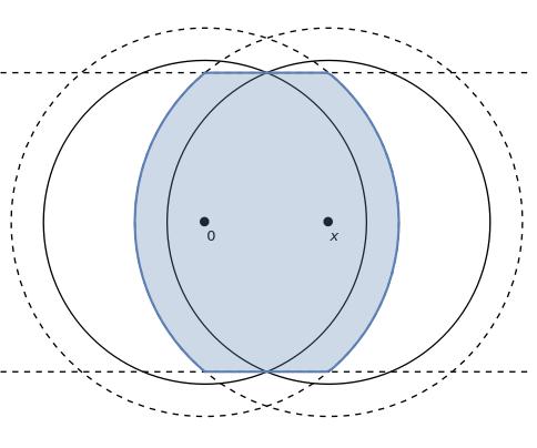
Figure 1. Set in the left-hand side of equation (19)

Indeed, the equations defining the left intersection are

(20) $$(a(y)+\cos(\alpha))^{2}+b(y)^{2}\leq(1+Mt)^{2},$$

(21) $$b(y)\leq\sin(\alpha).$$

If $a(y)\leq 2\cos(\alpha)$, then $(a(y)-\cos(\alpha))^{2}\leq\cos(\alpha)^{2}$ and we get from (21),

$$(a(y)-\cos(\alpha))^{2}+b(y)^{2}\leq 1.$$

If $a(y)\geq 2\cos(\alpha)$, we also get

(22) $$(a(y)-\cos(\alpha))^{2}+b(y)^{2} =(a(y)+\cos(\alpha))^{2}+b(y)^{2}-4a(y)\cos(\alpha)$$

(23) $$\leq(1+Mt)^{2}-4a(y)\cos(\alpha)$$

(24) $$\leq 1+8\cos(\alpha)^{2}-4a(y)\cos(\alpha)$$

(25) $$<1,$$

and this implies in both cases that

$$y\in B(0,1)\cup B(x,1)$$

and the claim is proven.

Notice that

$$B(0,1)\cup B(x,1)=L(x)\sqcup([0,1]_{S^{n-1}}^{x}\cap[1,\infty]_{S^{n-1}})\cap([0,1]_{S^{n-1}}\cap[1,\infty]_{S^{n-1}}^{x}).$$

Now, since both $G_{K_{t}}(x),L(K_{t},x)$ lie inside $B(0,1+Mt)\cap B(x,1+Mt)$, a point in either of the sets $U\cap G_{K_{t}}(x),U\cap L(K_{t},x)$ must belong to

(26) $$(B(0,1) \cup B(x,1))\cap(L(x)\sqcup[0,\infty]_{C(x)}\sqcup[0,\infty]_{C(-x)}^{x})$$

(27) $$=L(x)\sqcup([0,1]_{S^{n-1}}^{x}\cap[1,\infty]_{C(x)})\sqcup([0,1]_{S^{n-1}}\cap[1,\infty]_{C(-x)}^{x})$$

Inside this set, it is clear that the conditions defining $G_{K_{t}}(x)$ and $L(K_{t},x)$ coincide. To see this write $G_{K_{t}}(x)=[0,\rho_{K_{t}}]_{S^{n-1}}\cap[0,\rho_{K_{t}}]_{S^{n-1}}^{x}$ and

(28) $$G_{K_{t}}(x) \cap\left(L(x)\sqcup([0,1]_{S^{n-1}}^{x}\cap[1,\infty]_{C(x)})\sqcup([0,1]_{S^{n-1}}\cap[1,\infty]_{C(-x)}^{x})\right)$$

(29) $$=L(x)\sqcup([0,1]_{S^{n-1}}^{x}\cap[1,\rho_{K_{t}}]_{C(x)})\sqcup([0,1]_{S^{n-1}}\cap[1,\rho_{K_{t}}]_{C(-x)}^{x})$$

(30) $$L(K_{t},x) \cap\left(L(x)\sqcup([0,1]_{S^{n-1}}^{x}\cap[1,\infty]_{C(x)})\sqcup([0,1]_{S^{n-1}}\cap[1,\infty]_{C(-x)}^{x})\right).$$

Then, we only need to prove that

$$B(0,1+Mt)\cap B(x,1+Mt)\setminus U\subseteq T(ct).$$

The equations defining the left-hand side, are (20) and

(31) $$b(y)\geq\sin(\alpha).$$

From (20) we obtain

(32) $$a(y)^{2}+\cos(\alpha)^{2}+b(y)^{2}\leq(1+Mt)^{2},$$

and using (31) for $t<1$,

(33) $$a(y)^{2}\leq(1+Mt)^{2}-1=2Mt+M^{2}t^{2}\leq(2M+M^{2})t.$$

From (32) we also have

$$b(y)^{2}\leq(1+Mt)^{2}-\cos(\alpha)^{2}\leq(2M+M^{2})t+\sin(\alpha)^{2},$$

which yields, together with (33) and (31),

(34) $$(b(y)-\sin(\alpha))^{2}+a(y)^{2} =b(y)^{2}-2b(y)\sin(\alpha)+\sin(\alpha)^{2}+a(y)^{2}$$

(35) $$\leq(2M+M^{2})t+2\sin(\alpha)^{2}-2b(y)\sin(\alpha)+(2M+M^{2})t$$

(36) $$\leq 2(2M+M^{2})t$$

for $t\in(0,1)$.

On the other hand, the equations defining $S^{n-1}\cap(S^{n-1}+x)$ are

$$a(y)=0,b(y)=\sin(\alpha),$$

and the equations defining $T(ct)$ are

$$(b(y)-\sin(\alpha))^{2}+a(y)^{2}\leq ct.$$

Thus, we have proved that $B(0,1+Mt)\cap B(x,1+Mt)\setminus U\subseteq T(ct)$ for $t\in(0,t_{0})$, with $c=2(2M+M^{2})$ and some $t_{0}$ small, and the proof is complete.

∎

The following proposition guarantees that the computations of first and second derivatives in the next section are correctly justified.

Proposition 3.2.

Let $K$ be a $C^{\beta}$ radial set with $\beta\geq 1$. Then there is $\varepsilon>0$ such that the function

(37) $$S^{n-1}\times(-\varepsilon,\varepsilon)\times(0,2) \to\mathbb{R}$$

(38) $$(v,t,s) \mapsto g_{v}(t,s)=g_{K_{t}}(sv)$$

is $C^{\beta}$ smooth. Moreover, $\frac{\partial}{\partial s}g_{v}(t,s)\neq 0$.

Proof.

Fix $v_{0}\in S^{n-1},s_{0}\in(0,2)$. Since $K$ is $C^{\beta}$ and $\partial K_{0}=S^{n-1}$ intersects transversally with $\partial K_{0}+s_{0}v_{0}$, there is $\varepsilon>0$ small such that for all $(v,t,s)$ in an $\varepsilon$ neighborhood of $(v_{0},0,s_{0})$, the boundaries $\partial K_{t}$ and $\partial K_{t}+sv$ intersect transversally to each other, and to any line parallel to $v_{0}$ passing through a point in an $\varepsilon$ neighborhood of $G_{K_{t}}$.

Let $P_{v,t,s}$ be the orthogonal projection of $G_{K_{t}}(sv)$ onto the plane orthogonal to $v_{0}$, $\langle v_{0}\rangle^{\perp}$. By transversality, reducing $\varepsilon$ further if necessary, the set $G_{K_{t}}(sv)$ can be described as the region between the graphs of two functions $f_{-}$ and $f_{+}$. This is,

$$G_{K_{t}}(sv)=\{y+lv_{0}:y\in P_{v,t,s},f_{-}(v,t,y)+s\leq l\leq f_{+}(v,t,y)\}$$

for two $C^{\beta}$ functions $f_{\pm}$ defined for $(v,t)$ in a neighborhood of $(v_{0},0)$, and $y$ in a fixed open set containing $P_{v,t,s}$ for all such $(v,t,s)$. The volume can be computed as

(39) $$g_{v}(t,s) =\int_{P_{v,t,s}}(f_{+}(v,t,y)-f_{-}(v,t,y)-s)dy$$

(40) $$=\int_{S^{n-1}\cap\langle v_{0}\rangle^{\perp}}\int_{0}^{\rho(v,t,s)}r^{n-2}(f_{+}(v,t,r\xi)-f_{-}(v,t,r\xi)-s)drd\xi,$$

where $\rho(v,t,s)$ is the ($C^{\beta}$-smooth) radial function of $P_{v,t,s}$. Then it is clear that $g_{v}(t,s)$ is $C^{\beta}$ smooth around $(v_{0},0,s_{0})$.

By (39), the partial derivative with respect to $s$ is exactly $-{\left|P_{v,t,s}\right|}_{n-1}$, which is non-zero since $s\in(0,2)$ implies $G_{K_{t}}$ has non-empty interior. ∎

4. First-order Taylor Expansion of $C_{\delta}\overline{K_{t}}$

In order to compute the derivative of ${\left|C_{\delta}\overline{K_{t}}\right|}_{n}$ we need to compute that of the covariogram function.

Proposition 4.1.

Let $K$ be a radial set and $K_{t}$ be the radial body defined by (5), then for $x\in\mathbb{R}^{n}$ with $0<|x|<2$,

(41) $$g_{K_{t}}(x)={\left|L(x)\right|}_{n}+t\int_{S(x)}\rho_{K}(v)dv+O(t^{2}).$$

For $x=0$,

(42) $${\left|K_{t}\right|}_{n}={\left|\mathbb{B}\right|}_{n}+tI_{K}+O(t^{2}).$$

Here $\frac{O(t^{2})}{t^{2}}$ is bounded by a constant independent of $t\in(0,1)$ (but possibly depending on $K$ and $x$).

Proof.

Thanks to Proposition 3.1, the set $G_{K_{t}}(x)$ can be approximated as the disjoint union

(43) $$G_{K_{t}}(x)\sim[1,\rho_{K}]_{C(x)}\sqcup[1,\rho_{K}]_{C(-x)}^{x}\sqcup L(x)$$

where $A\sim B$ means that the symmetric difference $A\Delta B$ has volume $O(t^{2})$. Indeed, the symmetric difference must lie inside the torus $T(ct)$, whose volume is bounded by $c_{n}(ct)^{2}$ where $c_{n}$ is some dimensional constant.

We obtain

$$g_{K_{t}}(x)={\left|L(x)\right|}_{2}+{\left|[1,\rho_{K}]_{C(x)}\right|}_{2}+{\left|[1,\rho_{K}]_{C(-x)}\right|}_{2}+O(t^{2}).$$

Integrating in polar coordinates,

(44) $${\left|[1,\rho_{K}]_{C(x)}\right|}_{2} +{\left|[1,\rho_{K}]_{C(-x)}\right|}_{2}={\left|[1,\rho_{K}]_{S(x)}\right|}_{2}$$

(45) $$=\frac{1}{n}\int_{S(x)}(\rho_{K_{t}}(v)^{n}-1)dv$$

(46) $$=\frac{1}{n}\int_{S(x)}(nt\rho_{K}(v)+O(t^{2}))dv$$

(47) $$=t\int_{S(x)}\rho_{K}(v)dv+O(t^{2}),$$

and the proposition follows. ∎

Proof of Theorem 1.6.

For $t=0$, $\overline{K_{0}}$ is the Euclidean ball of volume $1$. The body $C_{\delta}\overline{K_{0}}$ is also a ball, and its radius $\rho_{0}$ satisfies $L(\rho_{0})=\delta$.

Start observing that for any $\lambda>0$,

$$g_{\lambda K}(\lambda x)=\lambda^{n}g_{K}(x),$$

implying that

$$g_{\bar{K}}(x)={\left|K\right|}_{n}^{-1}g_{K}({\left|K\right|}_{n}^{1/n}x).$$

Since $\rho_{C_{\delta}\overline{K_{t}}}(v)v$ is in the boundary of $C_{\delta}\overline{K_{t}}$, by the continuity of volume, the radial function $\rho_{C_{\delta}\bar{K}}(v)$ satisfies

$$\delta=g_{\overline{K_{t}}}(\rho_{C_{\delta}\overline{K_{t}}}(v)v)={\left|K_{t}\right|}_{n}^{-1}g_{K_{t}}({\left|K_{t}\right|}_{n}^{1/n}\rho_{C_{\delta}\overline{K_{t}}}(v)v).$$

We get

(48) $$\delta=k(t)^{-1}g_{v}(t,\rho_{v}(t)k(t)^{1/n}).$$

Clearly, for $t$ close to $0$, the function $k(t)$ is $C^{1}$ smooth and bounded away from $0$. By Proposition 3.2 and the Implicit Function Theorem, the function $\rho_{v}(t)$ must be $C^{1}$ with respect to $(t,v)$, in a neighborhood of $t=0$.

We can take derivative of (48) with respect to $t$, to obtain

(49) $$0 =-k(t)^{-2}k^{\prime}(t)g_{v}(t,\rho_{v}(t)k(t)^{1/n})$$

(50) $$+k(t)^{-1}\partial_{s}g_{v}(t,\rho_{v}(t)k(t)^{1/n})\left(\frac{1}{n}k(t)^{\frac{1}{n}-1}k^{\prime}(t)\rho_{v}(t)+k(t)^{1/n}\rho_{v}^{\prime}(t)\right)$$

(51) $$+k(t)^{-1}\partial_{t}g_{v}(t,\rho_{v}(t)k(t)^{1/n})$$

Notice that $g_{v}(0,s)=L(s)$ for every $s>0$, so $\partial_{s}g_{v}(0,s)=L^{\prime}(s)$. From (49) we compute

(52) $$\rho_{v}^{\prime}(0)=\omega_{n}^{-1/n}L^{\prime}(s_{0})^{-1}\left(\omega_{n}^{-1}k^{\prime}(0)L(s_{0})-\partial_{t}g_{v}(0,s_{0})\right)-\frac{1}{n}\omega_{n}^{-1}k^{\prime}(0)\rho_{0}$$

where $\omega_{n}=k(0)$ and $s_{0}=s(0)=\rho_{v}(0)k(0)^{1/n}$ is independent of $v$.

The volume of $C_{\delta}\overline{K_{t}}$ can be computed as

(53) $${\left|C_{\delta}\overline{K_{t}}\right|}_{n}=\frac{1}{n}\int_{S^{n-1}}\rho_{C_{\delta}\overline{K_{t}}}(v)^{n}dv$$

so taking derivative with respect to $t$ and using (52) and (42),

(54) $$\frac{\partial}{\partial t}{\left|C_{\delta}\overline{K_{t}}\right|}_{n}\bigg{|}_{t=0} =\rho_{0}^{n-1}\int_{S^{n-1}}\rho_{v}^{\prime}(0)dv$$

(55) $$=\rho_{0}^{n-1}\omega_{n}^{-1/n-1}I_{K}\frac{L(s_{0})}{L^{\prime}(s_{0})}n\omega_{n}-\frac{1}{n}\omega_{n}^{-1}I_{K}\rho_{0}^{n}n\omega_{n}$$

(56) $$-\rho_{0}^{n-1}\omega_{n}^{-1/n}L^{\prime}(s_{0})^{-1}\int_{S^{n-1}}\frac{\partial}{\partial t}g_{K_{t}}(s_{0}v)\bigg{|}_{t=0}dv.$$

By (41) in Proposition 4.1 we have $\frac{\partial}{\partial t}g_{K_{t}}(s_{0}v)\bigg{|}_{t=0}=W_{K,v}(s_{0})$. Observe that $S(x)$ is a union of two spherical caps, so for $v,w\in S^{n-1}$, we have $v\in S(s_{0}w)$ if and only if $w\in S(s_{0}v)$, then

(57) $$\int_{S^{n-1}}W_{K,v}(s_{0})dv =\int_{S^{n-1}}\int_{S^{n-1}}\chi_{S(s_{0}v)}(w)\rho_{K}(w)dwdv$$

(58) $$=\int_{S^{n-1}}\int_{S^{n-1}}\chi_{S(s_{0}w)}(v)dv\rho_{K}(w)dw$$

(59) $$=S(s_{0})I_{K}.$$

We get

(60) $$\frac{\partial}{\partial t}{\left|C_{\delta}\overline{K_{t}}\right|}_{n}\bigg{|}_{t=0} =\rho_{0}^{n-1}\omega_{n}^{-1/n}nI_{K}\frac{L(s_{0})}{L^{\prime}(s_{0})}-I_{K}\rho_{0}^{n}-\rho_{0}^{n-1}\omega_{n}^{-1/n}L^{\prime}(s_{0})^{-1}S(s)I_{K}$$

(61) $$=I_{K}L^{\prime}(s_{0})^{-1}\omega_{n}^{-1/n}\rho_{0}^{n-1}(nL(s_{0})-s_{0}L^{\prime}(s_{0})-S(s_{0})).$$

Finally we shall prove that

$$nL(s_{0})=s_{0}L^{\prime}(s_{0})+S(s_{0})$$

which concludes the proof.

Consider the $n-1$ dimensional circle $S_{2}=(\frac{1}{2}s_{0}v+v^{\perp})\cap(\mathbb{B}+s_{0}v)$ and observe that $L^{\prime}(s_{0})={\left|S_{2}\right|}_{n-1}$. Consider the cone $D_{2}$ with vertex at the origin and base $S_{2}$. Using the cone volume measure (see (9.33) of [13]), this is, $\frac{1}{n}|\langle n(x),x\rangle|dS(x)$ (where $n$ is a unit normal vector to the surface) to compute the volumes of the cones we get

(63) $$L(s_{0}) =2({\left|D(x)\right|}_{n}-{\left|D_{2}\right|}_{n})$$

(64) $$=\frac{2}{n}\left(\int_{C(x)}1dS(x)-\int_{S_{2}}\frac{s_{0}}{2}dS(x)\right)$$

(65) $$=\frac{2}{n}(\frac{1}{2}S(s)-\frac{s_{0}}{2}L^{\prime}(s_{0})).$$

and the proof is complete. ∎

5. Second-order Taylor Expansion of $C_{\delta}\overline{K_{t}}$ in the plane

In order to compute the second derivative of ${\left|C_{\delta}\overline{K_{t}}\right|}_{n}$ we need a second-order estimate of the covariogram of $K_{t}$. From now on, all computations will be made for $n=2$. We will make use of Proposition 3.1 again. In dimension $2$, the set $T(ct)$ is a union of two closed balls.

Proposition 5.1.

Let $K\subseteq\mathbb{R}^{2}$ be a planar radial set and $K_{t}$ be the radial body defined by (5), then

(66) $$g_{K_{t}}(x)=L(x)+t\int_{S(x)}\rho_{K}(v)dv+t^{2}\frac{1}{2}\int_{S(x)}\rho_{K}(v)^{2}dv+t^{2}T_{K}(x)+o(t^{2})\\$$

where $\frac{o(t^{2})}{t^{2}}\to 0$ as $t\to 0^{+}$, for fixed $K$ and $x$, and

(67) $$T_{K}(x)=\frac{1}{2|x|\sqrt{4-|x|^{2}}}\Big{(}4(\rho_{K}(v_{1})\rho_{K}(v_{2})+\rho_{K}(v_{3})\rho_{K}(v_{4}))\\ +(\rho_{K}(v_{1})^{2}+\rho_{K}(v_{2})^{2}+\rho_{K}(v_{3})^{2}+\rho_{K}(v_{4})^{2})(|x|^{2}-2)\Big{)}$$

where $(v_{1},v_{2})$ are the boundary points of $S(x)$ and $(v_{3},v_{4})$ are the lower ones, as shown in Figure 2(b).

Moreover,

(68) $${\left|K_{t}\right|}_{n}=\pi+tI_{K}+t^{2}{\left|K\right|}_{n}.$$

Proof.

Without loss of generality we may assume $x=(|x|,0)$. Let $p_{+},p_{-}$ be the upper and lower intersection points of $S^{1}$ and $S^{1}+x$. Proposition 3.1 provides constants $t_{0},c>0$ sufficiently small such that outside the balls $B(p_{\pm},ct)$, the sets in the left and right of (43) are equal for all $t\in[0,t_{0}]$. This is,

(69) $$G_{K_{t}}(x)\setminus B(p_{+},ct)\setminus B(p_{-},ct)\\ =\left(L(x)\sqcup[1,\rho_{K_{t}}]_{C(x)}\sqcup[1,\rho_{K_{t}}]_{C(-x)}^{x}\right)\setminus B(p_{+},ct)\setminus B(p_{-},ct).$$

(see Figure 2(a))

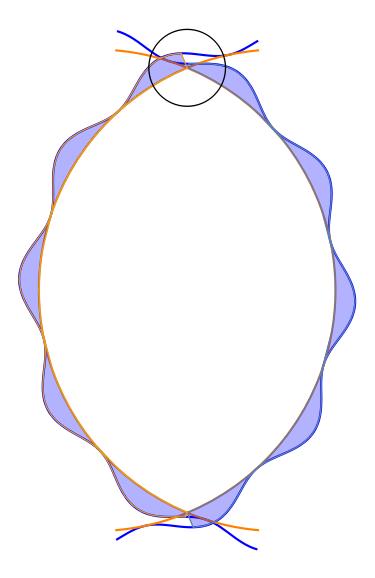
(a) Sets of equation (69) and $B(p_{+},ct)$.

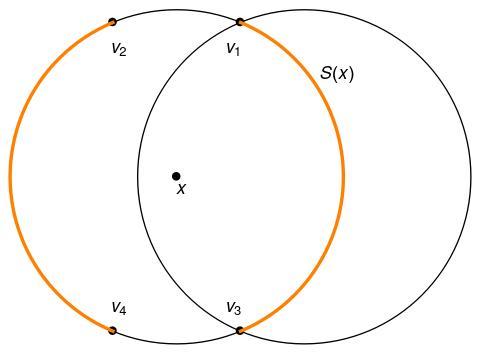
(b) Boundary points of $S(x)$,
$v_{1},v_{2},v_{3},v_{4}$

To simplify the computations, we will only compute the volume of $G_{K_{t}}(x)$ intersected with the upper half-plane $H^{+}$. For any measurable $A\subseteq\mathbb{R}^{2}$, we denote ${\left|A\right|}_{2+}={\left|A\cap H^{+}\right|}_{2}$. The intersection with the lower half-plane is similar and will be omitted. For small $t>0$, $B(p_{+},ct)$ lies in $H^{+}$.

To compute the second order term inside the ball we use a blow-up argument at the point $p_{+}$. The set

$$R_{1}(t)=\frac{1}{t}((G_{K_{t}}(x)\setminus L(x)\cap B(p_{+},ct))-p_{+})$$

is uniformly bounded with respect to $t$, and converges in the Hausdorff metric to

(70) $$R_{1}(0)=\Big{\{}y\in\mathbb{R}^{2}:|y|\leq d,\max\{y.v_{\alpha},y.v_{\pi-\alpha}\}\geq 0,\\ y.v_{\alpha}\leq\rho_{K}(\alpha),y.v_{\pi-\alpha}\leq\rho_{K}(\pi-\alpha)\Big{\}}$$

(see Figure 3(a)).

On the other hand, the set

$$R_{2}(t)=\frac{1}{t}\Big{(}([1,\rho_{K_{t}}]_{C(x)}\sqcup[1,\rho_{K_{t}}]_{C(-x)}^{x}-p_{+})\cap B(p_{+},ct)\Big{)}$$

is also uniformly bounded with respect to $t$ and converges in the Hausdorff metric to

(71) $$R_{2}(0)=\bigg{\{}y\in\mathbb{R}^{2}:|y|\leq d,(0\leq y.v_{\alpha}\leq\rho_{K}(v_{\alpha}),y.v_{\alpha-\pi/2}\geq 0)\\ \text{ or }(0\leq y.v_{\pi-\alpha}\leq\rho_{K}(v_{\pi-\alpha}),y.v_{\pi-\alpha+\pi/2}\geq 0)\bigg{\}}$$

(see Figure 3(c)).

We get from (69), (70), (71) and (47) that

(72) $$\Big{|}G_{K_{t}}(x)\Big{|}_{2+} ={\left|G_{K_{t}}(x)\setminus L(x)\setminus B(p_{+},ct)\right|}_{2+}+{\left|tR_{1}(t)\right|}_{2}+{\left|L(x)\right|}_{2+}$$

(73) $$={\left|\left([1,\rho_{K_{t}}]_{C(x)}\sqcup[1,\rho_{K_{t}}]_{C(-x)}^{x}\right)\setminus B(p_{+},ct)\right|}_{2+}+{\left|tR_{2}(t)\right|}_{2}+|L(x)|$$

(74) $$+t^{2}({\left|R_{1}(t)\right|}_{2}-{\left|R_{2}(t)\right|}_{2})$$

(75) $$={\left|[1,\rho_{K_{t}}]_{C(x)}\sqcup[1,\rho_{K_{t}}]_{C(-x)}^{x}\right|}_{2+}+{\left|L(x)\right|}_{2+}$$

(76) $$+t^{2}(R_{1}(0)-R_{2}(0))+o(t^{2})$$

(77) $$={\left|L(x)\right|}_{2+}+t\int_{S(x)\cap H_{+}}\rho_{K_{t}}(v)dv+\frac{1}{2}t^{2}\int_{S(x)\cap H_{+}}\rho_{K_{t}}(v)^{2}dv$$

(78) $$+t^{2}({\left|R_{1}(0)\right|}_{2}-{\left|R_{2}(0)\right|}_{2})+o(t^{2})$$

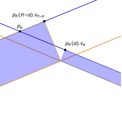
(a) Approximation of the set $R_{1}$ near $p_{+}$.

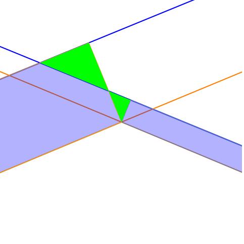
(b) Difference between $R_{1}$ and $R_{2}$.

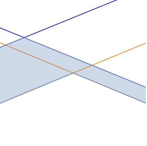
(c) Approximation of the set $R_{2}$ near $p_{+}$.

The difference ${\left|R_{1}(0)\right|}_{2}-{\left|R_{2}(0)\right|}_{2}$ is exactly the signed area of the quadrilateral with (ordered) vertices $0,\rho_{K_{t}}(\alpha)v_{\alpha},p_{\alpha},\rho_{K_{t}}(\pi-\alpha)v_{\pi-\alpha}$, where $p_{\alpha}$ is the intersection point of the two lines $p_{\alpha}\cdot v_{\alpha}=\rho_{K_{t}}(\alpha)$ and $p_{\alpha}\cdot v_{\pi-\alpha}=\rho_{K_{t}}(\pi-\alpha)$. The sign of the area of each region bounded by the quadrilateral is given by the sens of rotation of the boundary around it. (see Figure 3(b)) This quadrilateral is always convex if $\alpha\in(0,\pi/4)$. It is clear that this signed area is exactly $\frac{1}{2}(\det(\rho_{K_{t}}(\alpha)v_{\alpha},p_{\alpha})+\det(p_{\alpha},\rho_{K_{t}}(\pi-\alpha)v_{\pi-\alpha})$. By computing $p_{\alpha}$ in terms of $\alpha,\rho_{K_{t}}(\alpha)$ and $\rho_{K_{t}}(\pi-\alpha)$, and adding the corresponding term for the lower half space, we obtain the formula for $T_{K}(x)$.

The second formula is computed easily as

(79) $${\left|K_{t}\right|}_{n} =\frac{1}{2}\int_{S^{1}}\rho_{K_{t}}(v)^{2}dv$$

(80) $$=\frac{1}{2}\int_{S^{1}}(1+2t\rho_{K}(v)+t^{2}\rho_{K}(v)^{2})dv$$

(81) $$=\pi+t\int_{S^{1}}\rho_{K}(v)dv+t^{2}{\left|K\right|}_{n}.$$

∎

We are ready to compute the second derivative of the volume, in dimension $2$.

Proposition 5.2.

Let $K$ be a $C^{2}$ smooth radial set and $\overline{K_{t}}$ be defined by (6), then if $\alpha$ is given by (8),

(83) $$\frac{\partial^{2}}{\partial t^{2}}{\left|C_{\delta}\overline{K_{t}}\right|}_{2}\bigg{|}_{t=0} =\frac{1}{\pi\sin(\alpha)^{2}}\Biggl{(}-\frac{1}{2\pi}\left(\frac{\sin(2\alpha)-2\alpha}{\sin(\alpha)}\right)^{2}I_{K}^{2}$$

(84) $$-\frac{1}{2}\frac{\cos(\alpha)}{\sin(\alpha)}\int_{S^{1}}\left[\rho_{K}(v+\frac{\pi}{2}\pm\frac{\pi}{2}\pm\alpha)\right]w_{K,v}(\alpha)dv$$

(85) $$+\frac{1}{4\sin(\alpha)^{2}}\int_{S^{1}}\left(w_{K,v}(\alpha)\right)^{2}dv+2\int_{S^{1}}\rho_{K}(v-\alpha+\pi)\rho_{K}(v+\alpha)dv$$

(86) $$+4\cos(2\alpha){\left|K\right|}_{2}\Biggr{)}$$

where

$$\left[\rho_{K}(v+\frac{\pi}{2}\pm\frac{\pi}{2}\pm\alpha)\right]=\rho_{K}(v+\alpha)+\rho_{K}(v-\alpha)+\rho_{K}(v+\pi+\alpha)+\rho_{K}(v+\pi-\alpha).$$

Proof.

First we compute the second derivative of ${\left|C_{\delta}\overline{K_{t}}\right|}_{n}$ with respect to $t$ using (53), at $t=0$.

(87) $$\frac{\partial^{2}}{\partial t^{2}}{\left|C_{\delta}\overline{K_{t}}\right|}_{2}\bigg{|}_{t=0}=\int_{S^{1}}\rho_{v}^{\prime}(0)^{2}dv+\rho_{0}\int_{S^{1}}\rho_{K}^{\prime\prime}(0)dv.$$

In order to simplify the computations we write (48) as

(88) $$\delta=k(t)^{-1}g_{v}(t,s_{v}(t))$$

where $s_{v}(t)=k(t)^{1/2}\rho_{v}(t)$ and take derivative with respect to $t$ at $t=0$, to obtain

(89) $$s_{v}^{\prime}(0)=\frac{k_{0}^{\prime}g_{v,0}-k_{0}\partial_{t}g_{v,0}}{k_{0}\partial_{s}g_{v,0}}$$

where $g_{v,0}=g_{v}(0,s_{v}(0))$, $\partial_{t}g_{v,0}=\partial_{t}g_{v}(0,s_{v}(0))$. Take the second derivative of (88) with respect to $t$, at $t=0$, and use (89) to get

(90) $$s_{v}^{\prime\prime}(0) =\frac{1}{k_{0}^{2}\left(\partial_{s}g_{v,0}\right)^{3}}\Biggl{(}k_{0}g_{v,0}\left(-2k_{0}^{\prime}\partial_{s}g_{v,0}\partial_{t,s}g_{v,0}+2k_{0}^{\prime}\partial_{s,s}g_{v,0}\partial_{t}g_{v,0}+k_{0}^{\prime\prime}\left(\partial_{s}g_{v,0}\right)^{2}\right)$$

(91) $$-\left(\partial_{t}g_{v,0}\right)^{2}k_{0}^{2}\partial_{s,s}g_{v,0}+2k_{0}^{2}\partial_{s}g_{v,0}\partial_{t}g_{v,0}\partial_{t,s}g_{v,0}-k_{0}^{2}\left(\partial_{s}g_{v,0}\right)^{2}\partial_{t,t}g_{v,0}$$

(92) $$-\left(k_{0}^{\prime}\right)^{2}g_{v,0}^{2}\partial_{s,s}g_{v,0}\Biggr{)}$$

The terms $\rho_{v}^{\prime},\rho_{v}^{\prime\prime}$ can be computed from $s_{v}^{\prime},s_{v}^{\prime\prime}$ by the relation $s_{v}(t)=k(t)^{1/2}\rho_{v}(t)$ as

(93) $$\rho_{v}^{\prime}(0)=s_{v}^{\prime}(0)k_{0}^{-1/2}-\frac{1}{2}s_{v}(0)k_{0}^{-3/2}k_{0}^{\prime}\\$$

and

(94) $$\rho_{v}^{\prime\prime}(0)=-\frac{k_{0}^{\prime}s_{v}^{\prime}(0)}{k_{0}^{3/2}}+\frac{s_{v}^{\prime\prime}(0)}{\sqrt{k_{0}}}+\frac{3\left(k_{0}^{\prime}\right)^{2}\rho_{v}(0)}{4k_{0}^{2}}-\frac{k_{0}^{\prime\prime}\rho_{v}(0)}{2k_{0}}.$$

Using Propositions 4.1 and 5.1 we get the following identities:

(95) $$\begin{array}[]{ccc}k_{0}=\pi&k_{0}^{\prime}=I_{K}&k_{0}^{\prime\prime}=2{\left|K\right|}_{2}\\ g_{v,0}=L(s_{0})&\partial_{s}g_{v,0}=L^{\prime}(s_{0})&\partial_{s}g_{v,0}=L^{\prime\prime}(s_{0})\\ \end{array}$$

(96) $$\begin{array}[]{cc}\partial_{t}g_{v,0}=W_{K,v}(s_{0})&\partial_{t,t}g_{v,0}=\int_{S(s_{0}v)}\rho_{K}(w)^{2}dw+2T_{K}(s_{0}v)\\ \partial_{t,s}g_{v,0}=W_{K,v}^{\prime}(s_{0}).\end{array}$$

Notice that $g_{v,0},\partial_{s}g_{v,0},\partial_{s,s}g_{v,0}$ are independent of $v$.

Integrating (90),

(97) $$\int_{S^{1}}s_{v}^{\prime\prime}(0)dv =\frac{1}{\pi^{2}(L^{\prime})^{3}}\bigg{[}-2\pi I_{K}LL^{\prime}\int_{S^{1}}W_{K,v}^{\prime}dv+2\pi LI_{K}L^{\prime\prime}\int_{S^{1}}W_{K,v}dv$$

(98) $$+4\pi^{2}L{\left|K\right|}_{2}(L^{\prime})^{2}-\pi^{2}L^{\prime\prime}\int_{S^{1}}W_{K,v}^{2}dv-2\pi I_{K}^{2}L^{2}L^{\prime\prime}$$

(99) $$+\pi^{2}(L^{\prime})^{2}\int_{S^{1}}\Big{(}\int_{S(s_{0}v)}\rho_{K}(w)^{2}dw+2T_{K}(s_{0}v)\Big{)}dv$$

(100) $$+2\pi^{2}L^{\prime}\int_{S^{1}}W_{K,v}W_{K,v}^{\prime}dv\bigg{]}$$

where we omitted the argument $s_{0}$ in the functions $W_{K,v},W_{K,v}^{\prime},L,L^{\prime}$ and $L^{\prime\prime}$.

Using a computation similar to (57), we obtain

(101) $$\int_{S^{1}}\int_{S(s_{0}v)}\rho_{K}(w)^{2}dwdv=2S(s_{0}){\left|K\right|}_{2}.$$

Also from (57),

(102) $$\int_{S^{1}}W_{K,v}^{\prime}(s_{0})dv=S^{\prime}(s_{0})I_{K}.$$

We combine (87), (89), (90), (93), (94) the identities (95) and (96), and (101), (102), and we get

(103) $$\frac{\partial^{2}}{\partial t^{2}}{\left|C_{\delta}\overline{K_{t}}\right|}_{2}\bigg{|}_{t=0} =\frac{2}{\pi^{2}}\left(\frac{I_{K}L}{\pi^{3/2}L^{\prime}}\right)^{2}+\frac{1}{\pi(L^{\prime})^{2}}\int_{S^{1}}W_{K,v}^{2}dv+\frac{1}{2\pi}(\rho_{0}I_{K})^{2}$$

(104) $$-2\frac{I_{K}^{2}LS}{\pi^{2}(L^{\prime})^{2}}-\frac{2}{\pi^{3/2}}\frac{\rho_{0}I_{K}^{2}L}{L^{\prime}}+\frac{\rho_{0}}{\pi^{3/2}}\frac{I_{K}^{2}S}{L^{\prime}}+\rho_{0}\bigg{[}-\frac{1}{\pi^{3/2}}\frac{I_{K}^{2}L}{L^{\prime}}$$

(105) $$+\frac{I_{K}^{2}S}{\pi^{3/2}L^{\prime}}+\frac{1}{\pi^{1/2}}\int_{S^{1}}s_{v}^{\prime\prime}(0)dv+\frac{3}{2\pi}\rho_{0}I_{K}^{2}-2\rho_{0}{\left|K\right|}_{2}\bigg{]}.$$

We combine (103), with (97), (90), the identities (95) and (96), and after lengthy but straight-forward computations we get

(106) $$\frac{\partial^{2}}{\partial t^{2}}{\left|C_{\delta}\overline{K_{t}}\right|}_{2} \Big{|}_{t=0}=\frac{1}{\pi^{2}(L^{\prime})^{3}}\bigg{[}2\pi s_{0}L^{\prime}\left(\int_{S^{1}}W_{K,v}W_{K,v}^{\prime}dv\right)$$

(107) $$+\pi\left(L^{\prime}-s_{0}L^{\prime\prime}\right)\left(\int_{S^{1}}W_{K,v}^{2}dv\right)-2\pi s_{0}(L^{\prime})^{2}\left(\int_{S^{1}}T(v,s_{0})dv\right)$$

(108) $$-2\pi s_{0}^{2}|K|_{2}(L^{\prime})^{3}+4\pi s_{0}{\left|K\right|}_{2}L(L^{\prime})^{2}+2s_{0}^{2}I_{K}^{2}(L^{\prime})^{3}$$

(109) $$-2s_{0}I_{K}^{2}LS^{\prime}L^{\prime}+2s_{0}I_{K}^{2}SLL^{\prime\prime}+2s_{0}I_{K}^{2}S(L^{\prime})^{2}-2I_{K}^{2}SLL^{\prime}$$

(110) $$-2s_{0}I_{K}^{2}L^{2}L^{\prime\prime}-4s_{0}I_{K}^{2}L(L^{\prime})^{2}+2I_{K}^{2}L^{2}L^{\prime}-2\pi s_{0}S(L^{\prime})^{2}{\left|K\right|}_{2}\bigg{]}.$$

Now we parametrize with respect to the variable $\alpha\in(0,\pi/2)$ with $s_{0}=2\cos(\alpha)$. We have the following relations:

(111) $$\begin{array}[]{cccc}s_{0}=2\cos(\alpha)&\delta=L(s_{0})/\pi\\ S(s_{0})=4\alpha&S^{\prime}(s_{0})=-\frac{2}{\sin(\alpha)}\\ L^{\prime}(s_{0})=-2\sin(\alpha)&L^{\prime\prime}(s_{0})=\tan(\alpha)^{-1}&L(s_{0})=2(\alpha-\cos(\alpha)\sin(\alpha))\end{array}$$

To compute the term $W_{K,v}^{\prime}$, observe that

(112) $$-2\sin(\alpha) W_{K,v}^{\prime}(2\cos(\alpha))=w_{K,v}^{\prime}(\alpha)$$

(113) $$=\frac{\partial}{\partial\alpha}\left(\int_{v-\alpha}^{v+\alpha}\rho_{K}(w)dw+\int_{v+\pi-\alpha}^{v+\pi+\alpha}\rho_{K}(w)dw\right)$$

(114) $$=\rho_{K}(v+\alpha)+\rho_{K}(v-\alpha)+\rho_{K}(v+\pi+\alpha)+\rho_{K}(v+\pi-\alpha)$$

(115) $$=\left[\rho_{K}(v+\frac{\pi}{2}\pm\frac{\pi}{2}\pm\alpha)\right].$$

Using the identities (111) and (112) we simplify equation (106) to obtain (83).

∎

We are ready to compute the counterexample:

Proof of Theorem 1.8.

Consider the (infinitely smooth and symmetric) radial set given by

(116) $$\rho_{K^{m}}(v)=\cos(mv)^{2}=\frac{1}{2}\cos(2mv)+\frac{1}{2}.$$

(see Figure 4.)

Figure 4. The sets $K_{t}^{m}$ for $m=1,2,3,4$ and $t=\frac{1}{2m^{2}}$.

All integrals in (83) can be computed exactly using the two expressions for $\rho_{K^{m}}(v)$ in (116). To compute the last integral we use the identity

$$\cos(m(v-\alpha))^{2}\cos(m(v+\alpha))^{2}=\frac{1}{4}(\cos(2mv)+\cos(2m\alpha))^{2}.$$

Integrating every term in (83) we obtain

(117) $$I_{K}=\pi,\quad{\left|K\right|}_{2}=\frac{3}{8}\pi,\quad\int_{S^{1}}\rho_{K}(v-\alpha+\pi)\rho_{K}(v+\alpha)dv=\frac{1}{4}\pi(\cos(4\alpha m)+2)\\$$

(118) $$w_{K,v}(\alpha) =\frac{1}{4m}\left(\sin(2m(\alpha+v))+\sin(2m(\alpha+v+\pi))-2\sin(2m(v-\alpha))\right)$$

(119) $$\int_{S^{1}}w_{K,v}(\alpha)^{2}dv =\frac{\pi\left(16\alpha^{2}m^{2}-\cos(4\alpha m)+1\right)}{2m^{2}}$$

and

$$\int_{S^{1}}\left[\rho_{K}(v+\frac{\pi}{2}\pm\frac{\pi}{2}\pm\alpha)\right]w_{K,v}(\alpha)dv=\frac{1}{m}\pi(8\alpha m+\sin(4\alpha m)).$$

Denote $F_{m}(\alpha)=\frac{\partial^{2}}{\partial t^{2}}{\left|C_{\delta}\overline{K^{m}_{t}}\right|}_{2}\bigg{|}_{t=0}$, where $\delta$ and $\alpha$ are related by (8). Putting all the integrals together we get

(121) $$F_{m}(\alpha) =\frac{1}{\sin(\alpha)^{2}}\bigg{(}\frac{1}{2}\cos(2\alpha)+\frac{1}{2}\cos(4\alpha m)$$

(122) $$+\frac{1}{8m^{2}\sin^{2}(\alpha)}-\frac{\cos(4\alpha m)}{8m^{2}\sin^{2}(\alpha)}-\frac{\sin(4\alpha m)}{2m\tan(\alpha)}\bigg{)}.$$

Every pair $m,\alpha$ for which $F_{m}(\alpha)$ is positive will provide us a counterexample to Question 1.3. To finish the proof, it remains to prove that for every $\alpha_{0}\in(0,\pi/2)$ there exists $m$ such that $F_{m}(\alpha_{0})>0$.

Consider

$$c(\alpha,m)=\frac{1}{8m^{2}\sin(\alpha)^{2}}-\frac{\cos(4\alpha m)}{8m^{2}\sin^{2}(\alpha)}-\frac{\sin(4\alpha m)}{2m\tan(\alpha)}.$$

Equation (121) can be written as

$$\sin(\alpha)^{2}F_{S^{m}}(\alpha)=\frac{1}{2}\cos(2\alpha)+\frac{1}{2}\cos(4\alpha m)+c(\alpha,m).$$

(see Figure 5)

Figure 5. The function $\sin(\alpha)^{2}F_{m}(\alpha)$ for $m=10$.

The function $c(\alpha,m)$ tends to $0$ as $m\to\infty$, for every $\alpha\in(0,\pi/2]$.

Fix $\alpha_{0}\in(0,\pi/2)$ and consider $m_{0}$ such that for every $m\geq m_{0}$, $\frac{1}{2}\cos(2\alpha_{0})+c(\alpha_{0},m)>-1/2$. This is possible since $\cos(2\alpha_{0})\in(-1,1)$.

If $\alpha_{0}/\pi$ is a rational number, choose a suitable $m\geq m_{0}$ such that $\alpha_{0}m/\pi$ is integer, then $\cos(4m\alpha_{0})=1$. If $\alpha_{0}/\pi$ is not rational, the sequence $\cos(4m\alpha_{0}),m\geq m_{0}$ is dense in $[-1,1]$ and we may choose $m\geq m_{0}$ so that $\cos(4m\alpha_{0})$ is arbitrarily close to $1$.

In both cases we obtain at least one value of $m$ such that $F_{m}(\alpha_{0})>0$. ∎

Finally we are ready to give a negative answer to Question 1.3.

Proof of Theorem 1.9.

Let $\delta\in(0,1)$ and take the value of $\alpha$ given by the relations (111). By the proof of Theorem 1.8 there is $m\in\mathbb{N}$ such that $F_{m}(\alpha)>0$. Consider the radial set $K^{m}$ defined by (116) and the radial body $K^{m}_{t}=(K^{m})_{t}$ defined by (5). Since the function $\rho_{K^{m}_{t}}$ converges to $1$ in the $C^{\beta}$ topology for every $\beta\geq 0$, and since convexity is a $C^{2}$ property of $\rho$, there exists $\tilde{t}_{m}>0$ such that $K_{t}^{m}$ is convex for every $t\in[0,\tilde{t}_{m}]$ (by analyzing the Gauss curvature, one can see that $K_{t}^{m}$ is convex for $t\in[0,\frac{1}{2m^{2}}]$). By Theorems 1.6 and 1.8, there exists $t_{m}<\tilde{t}_{m}$ such that the function $t\mapsto{\left|C_{\delta}\overline{K^{m}_{t}}\right|}_{2}$ is increasing at $[0,\tilde{t}_{m}]$. Then

$${\left|C_{\delta}\overline{K^{m}_{t_{m}}}\right|}_{2}>{\left|C_{\delta}\overline{K^{m}_{0}}\right|}_{2}={\left|C_{\delta}\overline{\mathbb{B}}\right|}_{2},$$

and the proof is complete. ∎

6. The limit as $\delta\to 1$

In this section we prove Theorem 1.7. We split the proof in two parts: first we compute the limit as $\delta\to 1$, and later we show that the limit is non-positive.

Theorem 1.7 is a direct consequence of Propositions 6.1 and 6.2.

Proposition 6.1.

Let $K$ be a $C^{2}$ smooth radial set, then

(123) $$\lim_{\delta\to 1^{-}}\frac{1}{(1-\delta)^{2}}\frac{\partial^{2}}{\partial t^{2}}{\left|C_{\delta}\overline{K_{t}}\right|}_{2}\bigg{|}_{t=0} =\frac{3}{4}\pi\int_{S^{1}}\left(\frac{\rho_{K}(v)+\rho_{K}(v+\pi)}{2}\right)^{2}dv$$

(124) $$-\frac{1}{2}\left(\int_{S^{1}}\rho_{K}(v)dv\right)^{2}-\frac{\pi}{4}\int_{S^{1}}\rho_{K}^{\prime}(v)^{2}dv+\frac{\pi}{2}{\left|K\right|}_{n}.$$

Proof.

First notice that

$$\lim_{\alpha\to\pi/2^{-}}\frac{1-\delta}{\frac{4}{\pi}\cos(\alpha)}=1,$$

where $\delta$ and $\alpha$ are related by (8), so we may replace the factor $(1-\delta)^{2}$ in (124) by $(\frac{4}{\pi}\cos(\alpha))^{2}$. We rearrange some terms of (83) to obtain

(125) $$\frac{\pi\sin(\alpha)}{\cos(\alpha)^{2}} \frac{\partial^{2}}{\partial t^{2}}{\left|C_{\delta}\overline{K_{t}}\right|}_{2}\bigg{|}_{t=0}$$

(126) $$=\frac{1}{\sin(\alpha)}A_{1}(\alpha)+2A_{2}(\alpha)-\frac{1}{\sin(\alpha)^{2}}A_{3}(\alpha)+8{\left|K\right|}_{2}-\frac{2}{\pi}I_{K}^{2}$$

where

(127) $$A_{1}(\alpha) =\frac{1}{\cos(\alpha)}\left[\frac{4\alpha}{\pi}I_{K}^{2}-\frac{1}{2}\int_{S^{1}}\left[\rho_{K}(v+\frac{\pi}{2}\pm\frac{\pi}{2}\pm\alpha)\right]w_{K,v}(\alpha)dv\right]$$

(128) $$A_{2}(\alpha) =\frac{1}{\cos(\alpha)^{2}}\left[\int_{S^{1}}\rho_{K}(v-\alpha+\pi)\rho_{K}(v+\alpha)dv-\int_{S^{1}}\rho(v)^{2}dv\right]$$

(129) $$A_{3}(\alpha) =\frac{1}{\cos(\alpha)^{2}}\left[\frac{2\alpha^{2}}{\pi}I_{K}^{2}-\frac{1}{4}\int_{S^{1}}w_{K,v}(\alpha)^{2}dv\right].$$

Here we used the identities $\cos(2\alpha)=2\cos(\alpha)^{2}-1$ and $\sin(2\alpha)=2\sin(\alpha)\cos(\alpha)$. To compute the limits, first we observe that

$$\lim_{\alpha\to\pi/2^{-}}\frac{I_{K}-w_{K,v}(\alpha)}{2\pi-4\alpha}=\frac{1}{2}(\rho(v+\pi/2)+\rho(v-\pi/2)),$$

since the left term is the average of $\rho_{K}$ in the complement of $S(\cos(\alpha)v)$.

We compute $A_{1}$:

(130) $$\cos(\alpha) A_{1}(\alpha)=\frac{4\alpha}{\pi}I_{K}^{2}+\frac{1}{2}(2\pi-4\alpha)\int_{S^{1}}\left[\rho_{K}(v+\frac{\pi}{2}\pm\frac{\pi}{2}\pm\alpha)\right]\frac{I_{K}-w_{K,v}(\alpha)}{2\pi-4\alpha}dv$$

(131) $$-\frac{1}{2}\int_{S^{1}}\left[\rho_{K}(v+\frac{\pi}{2}\pm\frac{\pi}{2}\pm\alpha)\right]dvI_{K}$$

(132) $$=\frac{4}{\pi}I_{K}^{2}(\alpha-\pi/2)+2(\pi/2-\alpha)\int_{S^{1}}\left[\rho_{K}(v+\frac{\pi}{2}\pm\frac{\pi}{2}\pm\alpha)\right]\frac{I_{K}-w_{K,v}(\alpha)}{2\pi-4\alpha}dv.$$

Since $\frac{\cos(\alpha)}{\pi/2-\alpha}\to 1$ when $\alpha\to\pi/2$ we obtain

$$\lim_{\alpha\to\pi/2^{-}}A_{1}(\alpha)=8\int_{S^{1}}\left(\frac{\rho_{K}(v)+\rho_{K}(v+\pi)}{2}\right)^{2}dv-\frac{4}{\pi}I_{K}^{2}.$$

We compute $A_{2}$:

(133) $$\cos(\alpha)^{2} A_{2}(\alpha)=\int_{S^{1}}\rho_{K}(v-\alpha+\pi)\rho_{K}(v+\alpha)dv-\int_{S^{1}}\rho_{K}(v)^{2}dv$$

(134) $$=\frac{1}{2}\int_{S^{1}}(2\rho_{K}(v-\alpha+\pi)\rho_{K}(v+\alpha)dv-\rho_{K}(v+\alpha)^{2}-\rho_{K}(v-\alpha+\pi)^{2})dv$$

(135) $$=-2(\pi/2-\alpha)^{2}\int_{S^{1}}\left(\frac{\rho_{K}(v-\alpha+\pi)-\rho_{K}(v+\alpha)}{\pi-2\alpha}\right)^{2}dv$$

we get

$$\lim_{\alpha\to\pi/2^{-}}A_{2}(\alpha)=-2\int_{S^{1}}\rho_{K}^{\prime}(v)^{2}dv.$$

We compute $A_{3}$:

(137) $$\cos(\alpha)^{2} A_{3}(\alpha)=\frac{2\alpha^{2}}{\pi}I_{K}^{2}-\frac{1}{4}\int_{S^{1}}(w_{K,v}(\alpha)-I_{K})^{2}dv-\frac{1}{4}\int_{S^{1}}(2I_{K}w_{K,v}(\alpha)-I_{K}^{2})dv$$

(138) $$=I_{K}^{2}\left(\frac{2\alpha^{2}}{\pi}+\frac{\pi}{2}\right)-\frac{1}{2}I_{K}\int_{S^{1}}w_{K,v}(\alpha)dv$$

(139) $$-4\left(\frac{\pi}{2}-\alpha\right)^{2}\int_{S^{1}}\left(\frac{w_{K,v}(\alpha)-I_{K}}{2\pi-\alpha}\right)^{2}dv$$

(140) $$=I_{K}^{2}\left(\frac{2\alpha^{2}}{\pi}+\frac{\pi}{2}-2\alpha\right)-4\left(\frac{\pi}{2}-\alpha\right)^{2}\int_{S^{1}}\left(\frac{w_{K,v}(\alpha)-I_{K}}{2\pi-\alpha}\right)^{2}dv$$

(141) $$=\frac{2}{\pi}I_{K}^{2}\left(\frac{\pi}{2}-\alpha\right)^{2}-4\left(\frac{\pi}{2}-\alpha\right)^{2}\int_{S^{1}}\left(\frac{w_{K,v}(\alpha)-I_{K}}{2\pi-\alpha}\right)^{2}dv,$$

and we get

$$\lim_{\alpha\to\pi/2^{-}}A_{3}(\alpha)=\frac{2}{\pi}I_{K}^{2}-4\int_{S^{1}}\left(\frac{\rho_{K}(v)+\rho_{K}(v+\pi)}{2}\right)^{2}dv.$$

Putting together all the terms $A_{i}$ in (125), we get

(142) $$\lim\frac{\pi}{4\cos(\alpha)^{2}}\frac{\partial^{2}}{\partial t^{2}}{\left|C_{\delta}\overline{K_{t}}\right|}_{2}\bigg{|}_{t=0}=3\int_{S^{1}}\left(\frac{\rho_{K}(v)+\rho_{K}(v+\pi)}{2}\right)^{2}dv\\ -\frac{2}{\pi}\left(\int_{S^{1}}\rho_{K}(v)dv\right)^{2}-\int_{S^{1}}\rho_{K}^{\prime}(v)^{2}dv+2{\left|K\right|}_{n},$$

and the Proposition is proved. ∎

Finally, we shall prove that the limit of the second derivative is non-positive.

Proposition 6.2.

For every $C^{2}$ smooth radial set $K$,

(143) $$3\int_{S^{1}}\left(\frac{\rho_{K}(v)+\rho_{K}(v+\pi)}{2}\right)^{2}dv-\frac{2}{\pi}\left(\int_{S^{1}}\rho_{K}(v)dv\right)^{2}\\ -\int_{S^{1}}\rho_{K}^{\prime}(v)^{2}dv+2{\left|K\right|}_{n}\leq 0.$$

Equality holds if and only if

$$\rho_{K}(\alpha)=a+b\cos(\alpha)+c\sin(\alpha)+d\cos(2\alpha)+e\sin(2\alpha)$$

for some constants $a,b,c,d,e$.

Proof.

Since $\rho_{K}$ is a real periodic and continuous function we can represent it as a Fourier series

$$\rho_{K}(\alpha)=\sum_{n\in\mathbb{Z}}a_{n}e^{in\alpha}$$

with $a_{-n}=\overline{a_{n}},a_{0}>0$. The integrals are expressed as

(144) $$\int_{S^{1}}\rho_{K}=2\pi a_{0},\quad\int_{S^{1}}\rho_{K}^{2}=4\pi\sum_{n\geq 1}|a_{n}|^{2}+2\pi a_{0}^{2},\quad\int_{S^{1}}(\rho_{K}^{\prime})^{2}=4\pi\sum_{n\geq 1}n^{2}|a_{n}|^{2}$$

The symmetric part is

$$\frac{\rho_{K}(\alpha)+\rho_{K}(\alpha+\pi)}{2}=\sum_{n\in\mathbb{Z}}\varepsilon_{n}a_{n}e^{in\alpha}$$

where $\varepsilon_{n}=1$ if $n$ is even, and $\varepsilon_{n}=0$ if $n$ is odd. Using (144) we have

$$\int_{S^{1}}\left(\frac{\rho_{K}(v)+\rho_{K}(v+\pi)}{2}\right)^{2}dv=4\pi\sum_{n\geq 1}\varepsilon_{n}|a_{n}|^{2}+2\pi a_{0}^{2}$$

and we compute

(145) $$\lim\frac{\pi F(\alpha)}{4\cos(\alpha)^{2}} =3\left(4\pi\sum_{n\geq 1}\varepsilon_{n}|a_{n}|^{2}+2\pi a_{0}^{2}\right)-\frac{2}{\pi}(2\pi a_{0})^{2}$$

(146) $$-\left(4\pi\sum_{n\geq 1}n^{2}|a_{n}|^{2}\right)+\left(4\pi\sum_{n\geq 1}|a_{n}|^{2}+2\pi a_{0}^{2}\right)$$

(147) $$=12\pi\sum_{n\geq 1}\varepsilon_{n}|a_{n}|^{2}-4\pi\sum_{n\geq 1}n^{2}|a_{n}|^{2}+4\pi\sum_{n\geq 1}|a_{n}|^{2}$$

(148) $$=4\pi\left(\sum_{n\geq 1}(1+3\varepsilon_{n})|a_{n}|^{2}-\sum_{n\geq 1}n^{2}|a_{n}|^{2}\right)$$

Observe that $1+3\varepsilon_{n}\leq n^{2}$ for every $n\geq 1$, then the inequality follows.

Equality holds if and only if $a_{n}=0$ for all $|n|\geq 3$, which happens if and only if $K$ has radial function

$$\rho_{K}(\alpha)=a+b\cos(\alpha)+c\sin(\alpha)+d\cos(2\alpha)+e\sin(2\alpha).$$

This function is a homogeneous polynomial of degree $2$ in two variables, evaluated in $v_{\alpha}$. ∎

References

- [1] G. Averkov and G. Bianchi. Retrieving convex bodies from restricted covariogram functions. Advances in Applied Probability, 39(3):613–629, 2007.
- [2] G. Averkov and G. Bianchi. Confirmation of Matheron’s conjecture on the covariogram of a planar convex body. Journal of the European Mathematical Society, 11(6):1187–1202, 2009.
- [3] G. Bianchi. Matheron’s conjecture for the covariogram problem. Journal of the London Mathematical Society, 71(1):203–220, 2005.
- [4] K. J. Böröczky. Stronger versions of the Orlicz-Petty projection inequality. Journal of Differential Geometry, 95(2):215–247, 2013.
- [5] R. J. Gardner and G. Zhang. Affine inequalities and radial mean bodies. Amer. J. Math., 120(3):505–528, 1998.
- [6] J. Haddad and M. Ludwig. Affine fractional Sobolev and isoperimetric inequalities. arXiv, 2022.
- [7] J. Haddad and M. Ludwig. Affine Hardy–Littlewood–Sobolev inequalities. arXiv, 2023.
- [8] K. Kiener. Extremalität von ellipsoiden und die faltungsungleichung von Sobolev. Archiv der Mathematik, 46:162–168, 1986.
- [9] G. Matheron. Random Sets and Integral Geometry. Wiley Series in Probability and Statistics. Wiley, Michigan, 1975.
- [10] M. Meyer, S. Reisner, and M. Schmuckenschläger. The volume of the intersection of a convex body with its translates. Mathematika, 40(2):278–289, 1993.
- [11] C. M. Petty. Centroid surfaces. Pacific J. Math., 11:1535–1547, 1961.
- [12] M. Schmuckenschläger. The distribution function of the convolution square of a convex symmetric body in . Israel J. Math., 78(2-3):309–334, 1992.
- [13] R. Schneider. Convex Bodies: the Brunn-Minkowski Theory, volume 151 of Encyclopedia of Mathematics and its Applications. Cambridge University Press, Cambridge, Cambridge, UK, 2nd expanded edition, 2014.
- [14] A. Tsolomitis. Convolution bodies and their limiting behavior. Duke Mathematical Journal, 87:181–203, 1997.