Superluminal matter waves
Abstract
The Dirac equation has resided among the greatest successes of modern physics since its emergence as the first quantum mechanical theory fully compatible with special relativity. This compatibility ensures that the expectation value of the velocity is less than the vacuum speed of light. Here, we show that the Dirac equation admits free-particle solutions where the peak amplitude of the wavefunction can travel at any velocity, including those exceeding the vacuum speed of light, despite having a subluminal velocity expectation value. The solutions are constructed by superposing basis functions with correlations in momentum space. These arbitrary velocity wavefunctions feature a near-constant profile and may impact quantum mechanical processes that are sensitive to the local value of the probability density as opposed to expectation values.
The discovery of the Dirac equation stands as a foundational achievement of modern theoretical physics Dirac (1928). As the first quantum mechanical theory fully compatible with special relativity, the Dirac equation resolved several inconsistencies that beset the, otherwise widely successful, Schrödinger equation Schrödinger (1926). The equation and its solutions preserve many of the quantum mechanical concepts developed within the context of the Schrödinger equation, such as probability currents, expectation values, and operators. Unlike the Schrödinger equation, however, the Dirac equation was formulated from the outset to exhibit a Lorentz-invariant and Hamiltonian structure consistent with special relativity. In doing so, the Dirac equation precluded unphysical phenomena fully allowed by the Schrödinger equation: namely, expectation values for velocity that exceed the vacuum speed of light.
At a fundamental level, the Dirac equation is a wave equation. Within first quantization, the solutions, or wavefunctions , describe the quantum mechanical state of a charged lepton, while their adjoint product provides the probability density of finding the lepton within a particular region of space–time or momentum–energy. In the absence of fields (and vacuum nonlinearities), the simplest solution is a plane wave modulating a constant spinor Peskin and Schroeder (1995). Physically occurring, localized wavefunctions are typically formed by superposing these solutions with amplitudes and phases that are uncorrelated in space–time or momentum–energy. Superpositions featuring correlations in space–time or momentum–energy allow for wavefunctions with more-complex and potentially advantageous structures.
Insight into the fundamental properties of matter and light and the potential for applications has driven a growing interest in structured solutions for quantum mechanical and electromagnetic waves, with ideas from one often being adapted to the other Berry and Balazs (1979); Allen et al. (1992); Berry (1998); Bliokh et al. (2007); Verbeeck et al. (2010); Kaminer et al. (2012); Voloch-Bloch et al. (2013); Grillo et al. (2014); Kaminer et al. (2015); Lloyd et al. (2017); Hall and Abouraddy (2023); Campos et al. (2024); Chirita Mihaila et al. (2022); Wong et al. (2024). One of the most-iconic examples is the concept of orbital angular momentum from quantum mechanics being adapted to electromagnetism Allen et al. (1992); Berry (1998). Within quantum mechanics, this “wavefunction engineering” has been applied to: the formation of self-accelerating solutions, which appear to move under the influence of a potential in the absence of any potential Kaminer et al. (2015); Campos et al. (2024); transverse shaping of electron wavefunctions for added flexibility in scanning electron microscopes Chirita Mihaila et al. (2022); and the formation of free-electron crystals for enhancing x-ray radiation Wong et al. (2024). In each of these, the physical processes of interest are sensitive to the local properties of the wavefunction as opposed to expectation values.
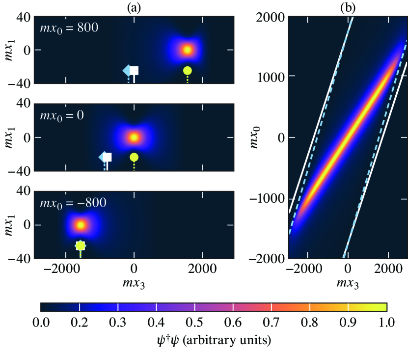
Here, we introduce a structured free-particle solution to the Dirac equation where the peak amplitude of the wavefunction can travel at any velocity, including those exceeding the vacuum speed of light, despite having a subluminal velocity expectation value (Fig. 1). Motivated by similar solutions found in electromagnetism (e.g., space–time wavepackets Longhi (2003); Kondakci and Abouraddy (2017); Yessenov et al. (2022) and flying focus pulses Sainte-Marie et al. (2017); Froula et al. (2018); Palastro et al. (2018); Di Piazza (2021); Formanek et al. (2023); Ramsey et al. (2023); Palastro et al. (2024)), the solutions feature a near-constant profile and are constructed by superposing basis functions with correlations in momentum–energy. We expect that the solutions, or approximations thereof, could be produced by light-matter interactions, such as the Kapitza–Dirac effect Kapitza and Dirac (1933); Freimund and Batelaan (2002); Shiloh et al. (2014); Grillo et al. (2014); Vanacore et al. (2018); Feist et al. (2020); Reinhardt and Kaminer (2020); García de Abajo and Konečná (2021); Lin et al. (2024), and generalized to exhibit more exotic properties, such as a modified effective mass in the absence of fields. These arbitrary velocity wavefunctions may impact quantum mechanical phenomena that are sensitive to the local value and velocity of the probability density, like Smith–Purcell or Cherenkov radiation Pupasov-Maksimov and Karlovets (2021), as opposed to expectation values.
The wavefunction of a spin one-half charged particle evolves according to the Dirac equation. In natural units (), the Schrödinger form of the Dirac equation is given by
| (1) |
where is the Hamiltonian,
the with are the Pauli matrices, is the identity matrix, and is the mass of the particle. Here and throughout, bold font denotes three-vectors, , the shorthand notations and are used for the momentum and position four-vectors, , and relativistic notation for sub and superscripts is not used.
The Dirac equation admits four plane wave solutions, corresponding to positive and negative energy and spin states. A general wavefunction can be expressed as a superposition of these solutions. For simplicity and definiteness, a superposition of solutions with positive energy and spin in the rest frame will be considered, such that
| (2) |
where
| (3) |
is the bispinor normalized so that , indicates a Hermitian conjugate, , , and the Dirac delta function ensures the “on-shell” condition. The complex scalar function determines the relative phase and amplitude of each plane wave that composes the wavefunction. Here, is expressed as an integral over an auxiliary parameter :
| (4) |
The utility of this auxiliary parameter will become clear below. The functions and are constrained by the normalization condition
| (5) |
where is the probability density and, for the remainder, is implied.
The evolution of the wavefunction can be characterized by three types of velocities: the phase velocities of the plane wave solutions, the eigenvalues (or expectation values) of the velocity operator, and the group velocity. The phase velocities, , are always superluminal (). The velocity operator is found by evaluating the commutator of the Hamiltonian and position vector: . Using Eq. (2), one finds , which, as expected, is always subluminal ().
The group velocity can take any value in any direction. For a typical wavefunction, the components of the four momenta must satisfy the on-shell condition but are otherwise independent. As a result, and
| (6) |
which is consistent with the eigenvalues of the velocity operator . However, if the momenta have some correlation, i.e., they are interdependent, then and
| (7) |
In this case, the correlated momenta introduce an additional contribution (the second term on the right-hand side) that decouples the group velocity from .
As an example, consider the case of an arbitrary, constant group velocity . Direct integration of yields
| (8) |
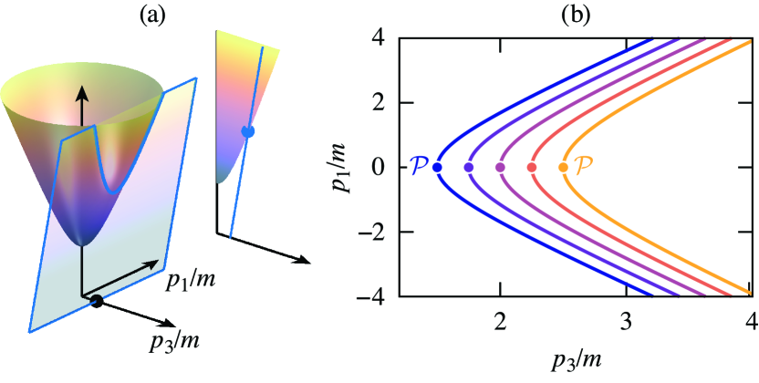
where is a constant. Setting ensures that the on-shell condition is satisfied and determines the interdependence of the momenta (Fig. 2). Specifically,
| (9) |
Without loss of generality, the specified group velocity will be aligned along the axis, i.e., , where denotes a unit vector. Substitution of Eqs. (8) and (9) into the right-hand-side of Eq. (7) verifies that indeed . The condition on the momenta [Eq. (9)] is a quadratic equation whose solution provides in terms of . Upon solving this equation, one finds
| (10) |
where . Note that only appears in even powers. Thus, a superluminal group velocity () does not produce a complex valued .
The interdependence of the momenta, as described by Eq. (10), can be built into the wavefunction by making use of the auxiliary parameter . Expressing as a function of (to be determined below) and setting
| (11) |
yields
| (12) |
where the dependence of and on is understood. Together, Eqs. (2) and (12) describe a superposition of solutions with correlated momenta parameterized by . Each solution has the same arbitrary group velocity .
To elucidate the physical meaning of the parameter and facilitate further calculation, it is helpful to substitute Eq. (12) into Eq. (2) and define the function
| (13) |
such that . Several properties of the arbitrary group velocity solutions can be analyzed by considering the phase in Eq. (13): . Making use of the delta function, the phase contribution becomes
| (14) |
The first term is proportional to but does not depend on . As a result, the factor can be extracted from the integrand. This factor shows that quantifies the temporal phase advance of the wavefunction. The second term in Eq. (14) reveals that the integrand depends on and only in the combination . Thus, the integrand advects at the group velocity .
An intuitive, and often helpful, picture of a wavefunction is that of an “envelope” modulated by a “carrier” wave. The envelope describes the bulk motion of the probability density and propagates at the group velocity, while the carrier describes the motion of the phase fronts, which propagate at the phase velocity. The function can be expressed in this same framework. Adding and subtracting a longitudinal (along ) momentum offset to Eq. (14) provides
| (15) |
With this offset, the first and second terms in describe the phase of the carrier wave, which can be extracted from the integrand as before, and the advection of the integrand (i.e., the envelope) at the group velocity. Choosing
| (16) |
where , yields
| (17) |
and ensures that the phase fronts of the carrier wave travel at a phase velocity . Note that this is equivalent to the procedure of enveloping the wavefunction about the longitudinal momentum and energy .
With the auxiliary parameter , the condition on the interdependence of the momenta [Eq. (10)] simplifies to
| (18) |
where the choice of sign ensures that the envelope varies slowly compared to the phase fronts. Equation (18) demonstrates two important points: First and foremost that corresponds to the value of when . And second that arbitrary group velocity solutions are precluded in one dimension. In one dimension, the wavefunction is composed solely of plane waves with , such that is always equal to . This eliminates the second term in Eq. (17), which is responsible for the movement of the envelope at . Figure 2(b) displays a family of longitudinal momenta [Eq. (18)] parameterized by as a function of perpendicular momentum for a superluminal group velocity .
A distinguishing property of the Dirac equation is its Lorentz covariance. Lorentz transformations of the arbitrary group velocity solutions [Eqs. (13) and (18)] provides additional insight into their interpretation. Upon performing a longitudinal Lorentz transformation to a frame moving at a velocity with respect to the nominal frame, Eq. (17) becomes
| (19) | ||||
where ′ denotes coordinates in the moving frame and is the nominal phase velocity in the moving frame. One may expect that would be a natural choice for the frame velocity. However, special care must be taken to ensure that the nominal phase velocity is always superluminal (i.e., the on-shell condition is satisfied). For , one can indeed set to find
| (20) |
but for the on-shell condition requires , which yields
| (21) |
Recall that the second terms in Eqs. (20) and (21) determine the space–time dependence of the envelope. Thus, the subluminal and superluminal solutions represent Lorentz transformations of solutions with time-independent and longitudinal-coordinate-independent envelopes, respectively.
The phase [Eq. (17)] and momentum condition [Eq. (18)] appearing in Eq. (13) depend directly on . Thus, a convenient choice for the auxiliary parameter is , or more explicitly [see Eq. (16)]. Using this choice and applying the delta functions in Eq. (13) provides
| (22) | ||||
where , ,
and the dependence of , , and are understood. As before, the integral (envelope) depends solely on the space–time coordinates in the combination and advects at .
Approximate analytical solutions for , and ultimately , can be found for a particle moving predominantly in the direction with a velocity that is sufficiently distinct from the group velocity . More specifically, one assumes , where is the transverse momentum spread. This condition describes a “paraxial” limit in which Eq. (18) simplifies to
| (23) |
With the quadratic dependence of on , a natural choice of basis functions for are the Laguerre–Gaussian modes:
| (24) |
where , is a generalized Laguerre polynomial, and is the azimuth in momentum space. Upon substituting Eqs. (23) and (24) into Eq. (22), dropping terms higher order than in the spinor, and integrating, one finds
| (25) |
where . Each component of the spinor can be expressed in terms of as follows:
| (26) | ||||
where , is the azimuth in configuration space, , , and
| (27) |
Equations (25) – (27) show that the envelope advects at the group velocity while maintaining a constant profile characterized by the duration .
The quantify the distribution of values for every and mode that compose the wavefunction. Said differently, the wavefunction is comprised of solutions that fall along a curve defined by Eq. (23) and parameterized by [Fig. 2(b)]: . If the are narrowly peaked about some , an approximate expression for this integral and the wavefunction can be obtained. Expressing yields
| (28) |
where , , and . Figure 1 displays the components of a wavefunction with a superluminal velocity for and .
Solutions to the Dirac equation can feature a peak probability density that moves at any velocity, including those exceeding the speed of light, while maintaining a near-constant profile. This motion is independent of the velocity expectation value. The solutions are on-shell and constructed by superposing basis functions with correlations in the longitudinal and transverse momenta. Future work will investigate electromagnetic structures that can produce these wavefunctions through the Kapitza–Dirac effect; explore the benefit of these wavefunctions in phenomena, such as Compton scattering and Smith–Purcell and Cherenkov radiation; and pursue additional structures by replacing Eq. (8) with other dependencies, like , which could exhibit classical dispersion with a modified effective mass in vacuum.
Acknowledgements.
The authors would like to thank R. R. Almeida and D. H. Froula for insightful discussions. The work of M.F. is supported by the European Union’s Horizon Europe research and innovation program under the Marie Skłodowska-Curie Grant Agreement No. 101105246-STEFF. The work of J.P.P., D.R., and A.D. is supported by the Office of Fusion Energy Sciences under Award Numbers DE-SC0021057, the Department of Energy National Nuclear Security Administration under Award Number DE-NA0004144, the University of Rochester, and the New York State Energy Research and Development Authority. This report was prepared as an account of work sponsored by an agency of the US Government. Neither the US Government nor any agency thereof, nor any of their employees, makes any warranty, express or implied, or assumes any legal liability or responsibility for the accuracy, completeness, or usefulness of any information, apparatus, product, or process disclosed, or represents that its use would not infringe privately owned rights. Reference herein to any specific commercial product, process, or service by trade name, trademark, manufacturer, or otherwise does not necessarily constitute or imply its endorsement, recommendation, or favoring by the US Government or any agency thereof. The views and opinions of authors expressed herein do not necessarily state or reflect those of the US Government or any agency thereof.References
- Dirac (1928) P. Dirac, Proceedings of the Royal Society of London. Series A, Containing Papers of a Mathematical and Physical Character 117, 610–624 (1928).
- Schrödinger (1926) E. Schrödinger, Phys. Rev. 28, 1049 (1926).
- Peskin and Schroeder (1995) M. Peskin and D. Schroeder, An Introduction To Quantum Field Theory, Frontiers in Physics (Avalon Publishing, 1995).
- Berry and Balazs (1979) M. V. Berry and N. L. Balazs, American Journal of Physics 47, 264 (1979).
- Allen et al. (1992) L. Allen, M. W. Beijersbergen, R. J. C. Spreeuw, and J. P. Woerdman, Phys. Rev. A 45, 8185 (1992).
- Berry (1998) M. V. Berry, in International Conference on Singular Optics, Vol. 3487, edited by M. S. Soskin, International Society for Optics and Photonics (SPIE, 1998) pp. 6 – 11.
- Bliokh et al. (2007) K. Y. Bliokh, Y. P. Bliokh, S. Savel’ev, and F. Nori, Phys. Rev. Lett. 99, 190404 (2007).
- Verbeeck et al. (2010) J. Verbeeck, H. Tian, and P. Schattschneider, Nature 467, 301 (2010).
- Kaminer et al. (2012) I. Kaminer, R. Bekenstein, J. Nemirovsky, and M. Segev, Phys. Rev. Lett. 108, 163901 (2012).
- Voloch-Bloch et al. (2013) N. Voloch-Bloch, Y. Lereah, Y. Lilach, A. Gover, and A. Arie, Nature 494, 331 (2013).
- Grillo et al. (2014) V. Grillo, E. Karimi, G. C. Gazzadi, S. Frabboni, M. R. Dennis, and R. W. Boyd, Phys. Rev. X 4, 011013 (2014).
- Kaminer et al. (2015) I. Kaminer, J. Nemirovsky, M. Rechtsman, R. Bekenstein, and M. Segev, Nature Physics 11, 261 (2015).
- Lloyd et al. (2017) S. M. Lloyd, M. Babiker, G. Thirunavukkarasu, and J. Yuan, Rev. Mod. Phys. 89, 035004 (2017).
- Hall and Abouraddy (2023) L. A. Hall and A. F. Abouraddy, Nature Physics 19, 435 (2023).
- Campos et al. (2024) A. G. Campos, K. Z. Hatsagortsyan, and C. H. Keitel, Phys. Rev. Res. 6, 023040 (2024).
- Chirita Mihaila et al. (2022) M. C. Chirita Mihaila, P. Weber, M. Schneller, L. Grandits, S. Nimmrichter, and T. Juffmann, Phys. Rev. X 12, 031043 (2022).
- Wong et al. (2024) L. W. W. Wong, X. Shi, A. Karnieli, J. Lim, S. Kumar, S. Carbajo, I. Kaminer, and L. J. Wong, Light: Science & Applications 13, 29 (2024).
- Longhi (2003) S. Longhi, Phys. Rev. E 68, 066612 (2003).
- Kondakci and Abouraddy (2017) H. E. Kondakci and A. F. Abouraddy, Nature Photonics 11, 733 (2017).
- Yessenov et al. (2022) M. Yessenov, J. Free, Z. Chen, E. G. Johnson, M. P. J. Lavery, M. A. Alonso, and A. F. Abouraddy, Nature Communications 13, 4573 (2022).
- Sainte-Marie et al. (2017) A. Sainte-Marie, O. Gobert, and F. Quéré, Optica 4, 1298 (2017).
- Froula et al. (2018) D. H. Froula, D. Turnbull, A. S. Davies, T. J. Kessler, D. Haberberger, J. P. Palastro, S.-W. Bahk, I. A. Begishev, R. Boni, S. Bucht, J. Katz, and J. L. Shaw, Nature Photonics 12, 262 (2018).
- Palastro et al. (2018) J. P. Palastro, D. Turnbull, S.-W. Bahk, R. K. Follett, J. L. Shaw, D. Haberberger, J. Bromage, and D. H. Froula, Phys. Rev. A 97, 033835 (2018).
- Di Piazza (2021) A. Di Piazza, Phys. Rev. A 103, 012215 (2021).
- Formanek et al. (2023) M. Formanek, J. P. Palastro, M. Vranic, D. Ramsey, and A. Di Piazza, Phys. Rev. E 107, 055213 (2023).
- Ramsey et al. (2023) D. Ramsey, A. D. Piazza, M. Formanek, P. Franke, D. H. Froula, B. Malaca, W. B. Mori, J. R. Pierce, T. T. Simpson, J. Vieira, M. Vranic, K. Weichman, and J. P. Palastro, Physical Review A 107, 013513 (2023).
- Palastro et al. (2024) J. P. Palastro, K. G. Miller, R. K. Follett, D. Ramsey, K. Weichman, A. V. Arefiev, and D. H. Froula, Phys. Rev. Lett. 132, 095101 (2024).
- Kapitza and Dirac (1933) P. L. Kapitza and P. A. M. Dirac, Mathematical Proceedings of the Cambridge Philosophical Society 29, 297–300 (1933).
- Freimund and Batelaan (2002) D. L. Freimund and H. Batelaan, Phys. Rev. Lett. 89, 283602 (2002).
- Shiloh et al. (2014) R. Shiloh, Y. Lereah, Y. Lilach, and A. Arie, Ultramicroscopy 144, 26 (2014).
- Vanacore et al. (2018) G. M. Vanacore, I. Madan, G. Berruto, K. Wang, E. Pomarico, R. J. Lamb, D. McGrouther, I. Kaminer, B. Barwick, F. J. García de Abajo, and F. Carbone, Nature Communications 9, 2694 (2018).
- Feist et al. (2020) A. Feist, S. V. Yalunin, S. Schäfer, and C. Ropers, Phys. Rev. Res. 2, 043227 (2020).
- Reinhardt and Kaminer (2020) O. Reinhardt and I. Kaminer, ACS Photonics 7, 2859 (2020).
- García de Abajo and Konečná (2021) F. J. García de Abajo and A. Konečná, Phys. Rev. Lett. 126, 123901 (2021).
- Lin et al. (2024) K. Lin, S. Eckart, H. Liang, A. Hartung, S. Jacob, Q. Ji, L. P. H. Schmidt, M. S. Schöffler, T. Jahnke, M. Kunitski, and R. Dörner, Science 383, 1467 (2024).
- Pupasov-Maksimov and Karlovets (2021) A. Pupasov-Maksimov and D. Karlovets, New Journal of Physics 23, 043011 (2021).