Leveraging Active Subspaces to Capture Epistemic Model Uncertainty in Deep Generative Models for Molecular Design

Abstract

Deep generative models have been accelerating the inverse design process in material and drug design. Unlike their counterpart property predictors in typical molecular design frameworks, generative molecular design models have seen fewer efforts on uncertainty quantification (UQ) due to computational challenges in Bayesian inference posed by their large number of parameters. In this work, we focus on the junction-tree variational autoencoder (JT-VAE), a popular model for generative molecular design, and address this issue by leveraging the low dimensional active subspace to capture the uncertainty in the model parameters. Specifically, we approximate the posterior distribution over the active subspace parameters to estimate the epistemic model uncertainty in an extremely high dimensional parameter space. The proposed UQ scheme does not require alteration of the model architecture, making it readily applicable to any pre-trained model. Our experiments demonstrate the efficacy of the AS-based UQ and its potential impact on molecular optimization by exploring the model diversity under epistemic uncertainty.

Index Terms—  Bayesian Inference, Active Subspace (AS), Uncertainty Quantification (UQ), Generative Molecular Design (GMD), Junction Tree Variational Autoencoder (JT-VAE)

1 Introduction

Due to the advancement in deep learning, particularly in generative models, there has been increased application of generative design in material and drug discovery tasks. In small molecular drug design domain, different generative models [1, 2, 3, 4, 5, 6] are used for inverse design of molecules in conjunction with optimization strategies including Bayesian optimization, gradient ascent etc. In particular the generative molecular design (GMD) models like the Junction Tree Variational Autoencoder (JT-VAE) [3] allow designing molecules with desired properties without directly optimizing over massive chemical space by embedding the molecules to a continuous and low dimensional latent space representation from high dimensional discrete chemical space.

Although the use of deep generative models in molecular design is on the rise, uncertainty of these large neural networks is relatively less explored in this domain. The existing works [7, 8, 9, 10] primarily focus on the uncertainty of the classifier or regressor for molecular property prediction since the predicted properties of designed molecules often guide the inverse design process. Uncertainty quantification of the generative models that produce these molecules can lead to more robust application of the generative models in drug design. [11] demonstrated that epistemic uncertainty of the decoder in variational autoencoder (VAE) can enhance the efficiency of molecule generation task by enabling uncertainty aware optimization approach over the latent space.

Bayesian inference [12, 13] technique is successfully used for capturing the uncertainty in predictions from the molecular property predictors [8]. However, due to the large parameter space of generative molecular design models, e.g. JT-VAE (5.7M parameters), it is computationally challenging to learn the high dimensional posterior distribution over the generative model parameters. Earlier efforts in Bayesian framework to address this issue trace back to the introduction of effective dimensionality of neural network parameter space in [12]. [14] found that many directions in parameter space near local optima minimally impact neural network predictions. On one hand, [15] established that the heavily parameterized DNNs can be pruned leading to subnetworks with comparable performance. Accordingly, several pruning approaches in Bayesian deep learning lead to a substantially small subnetwork for tractable UQ [16, 17, 18, 19]. On the other hand, inference over a low-dimensional subspace of the weights can effectively capture model uncertainty [20, 21]. In this work, we proposed the use of active subspace [21] to quantify the epistemic uncertainty of JT-VAE model parameters where low dimensional active subspace facilitates the approximation of the posterior distribution using variational inference. Specifically, we use active subspace inference for its plug-n-play advantage over other subspace methods as we only need to collect small number of gradient samples from model weight perturbations to construct the subspace. Since the proposed approach does not require any change in the architecture of JT-VAE model unlike the dropout method for Bayesian approximation [22], it can be used as a plug-in tool for quantifying the uncertainty of GMD model in the established molecular design pipeline.

Our main contribution can be summarized as:

• We construct a low dimensional active subspace for capturing epistemic uncertainty of JT-VAE model which is otherwise computationally challenging due to its high-dimensional parameter space.

• We additionally perform active subspace inference over all four components of JT-VAE parameters – graph encoder, tree encoder, graph decoder, and tree decoder – separately to demonstrate the effectiveness of our approach in improving the predictive UQ compared to the pre-trained JT-VAE model.

• We further investigate the impact of our active subspace inference over JT-VAE on its generated molecules in terms of 6 different molecular properties of interest.

2 Methodology

2.1 Junction Tree Variational Autoencoder (JT-VAE)

The Junction Tree Variational Autoencoder or JT-VAE [3] is a variational autoencoder based generative model that is used for several molecular design applications [1]. This model utilizes two different representations of input molecule – molecular graph and its corresponding junction tree. The graph encoder projects the molecular graph to a 28-dimensional latent representation. Similarly, we have 28-dimensional latent vectors for the junction tree encoded by the tree encoder. The molecular graph embedding and the junction tree embedding together form the 56-dimensional latent space of JT-VAE.

A two-stage procedure is followed to reconstruct the molecule from its latent space representation. First, the tree decoder decodes the junction tree embedding to a set of sequential decision rules needed to reconstruct the corresponding junction tree iteratively. Next, based on the reconstructed junction tree, the graph decoder utilizes the graph embedding component in the latent vector to build the molecular graph. The JT-VAE model is trained by minimizing the reconstruction loss for the junction tree and the molecular graph and the KL divergence loss between the posterior and prior distribution over the 56-dimensional latent space. The detailed description of the JT-VAE model architecture as well as the decoding process from latent vector can be found in [3].

2.2 Quantifying Uncertainty of JT-VAE Parameters

Our goal is to quantify the epistemic uncertainty of JT-VAE model, $p(\boldsymbol{\theta}|\mathcal{D})$ which indicates the uncertainty about the model parameters after it is trained with the training dataset $\mathcal{D}$. However, directly learning this distribution over the parameters is computationally challenging due to the high dimensionality of JT-VAE parameter space. In this work, we leverage the low dimensionality of active subspace to capture this uncertainty of JT-VAE. Specifically, we first construct the active subspace around the pre-trained JT-VAE model parameters followed by approximation of the posterior distribution over active subspace parameters. Finally, the samples from the learned posterior distribution are transformed to the original high dimensional parameter space of JT-VAE.

The quantified epistemic uncertainty can improve the predictive performance of JT-VAE. The pre-trained JT-VAE model parameters are the maximum likelihood estimate found by minimizing the training loss. Having a distribution over parameters instead of this point estimate helps the JT-VAE model to have better predictive uncertainty since it makes the model more robust to diverse set of training molecules.

2.3 Active Subspace of Deep Neural Network

In order to reduce the high dimensionality of a DNN model, we employ the active subspace (AS) of the model parameters similar to [21]. We identify a low-dimensional subspace, $\boldsymbol{\Omega}$ within a high-dimensional parameter space $\boldsymbol{\Theta}$ (Figure 1) that most significantly influences the variability in the DNN’s output on average. First we consider a continuous function $f_{\boldsymbol{\theta}}(\boldsymbol{x})$ with $\boldsymbol{x}$ and $\boldsymbol{\theta}\in\mathbb{R}^{D}$ denoting the input and the model parameters respectively. The parameters are stochastic with $\boldsymbol{\theta}\sim p(\boldsymbol{\theta})$ being their probability distribution. We then construct a $D\times D$ uncentered covariance matrix of the gradient of $f_{\boldsymbol{\theta}}(\boldsymbol{x})$: $\mathcal{C}=\mathbb{E}_{\boldsymbol{\theta}}\left[(\nabla_{\boldsymbol{\theta}}f_{\boldsymbol{\theta}}(\boldsymbol{x}))(\nabla_{\boldsymbol{\theta}}f_{\boldsymbol{\theta}}(\boldsymbol{x}))^{T}\right]$ which can be approximated using Monte Carlo sampling as follows:

$$\hat{\mathcal{C}}=\frac{1}{n}\sum_{i=1}^{n}(\nabla_{\boldsymbol{\theta}_{i}}f_{\boldsymbol{\theta}_{i}}(\boldsymbol{x}))(\nabla_{\boldsymbol{\theta}_{i}}f_{\boldsymbol{\theta}_{i}}(\boldsymbol{x}))^{T},\enskip\enskip\boldsymbol{\theta}_{i}\sim p(\boldsymbol{\theta})$$ (1)

where we generally have number of parameters, $D\gg n$. Now suppose $\hat{\mathcal{C}}$ follows the eigendecomposition: $\hat{\mathcal{C}}=\boldsymbol{V}\boldsymbol{\Lambda}\boldsymbol{V}^{T}$ where $\boldsymbol{V}$ contains all the eigenvectors and $\boldsymbol{\Lambda}=\rm{diag}(\lambda_{1},\dots,\lambda_{D})$ are the eigenvalues with $\lambda_{1}\geq\dots\lambda_{D}\geq 0$. To extract subspace with most influential active directions, we split $\boldsymbol{V}$ in two parts $[\boldsymbol{V}_{1},\boldsymbol{V}_{2}]$ where $\boldsymbol{V}_{1}\in\mathbb{R}^{D\times k}$ and $\boldsymbol{V}_{2}\in\mathbb{R}^{D\times(D-k)}$ with $k\leq n\ll D$. The subspace spanned by $\boldsymbol{V}_{1}$ corresponds to the $k$ largest eigenvalues in $\boldsymbol{\Lambda}$ and is considered as the “active” subspace. Accordingly, the projection matrix to reconstruct the model parameters from the subspace parameters is $\mathbf{P}=\boldsymbol{V}_{1}$.

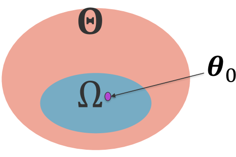
Fig. 1: Low dimensional active subspace $\boldsymbol{\Omega}$ around the pre-trained DNN parameter $\boldsymbol{\theta}_{0}\in\boldsymbol{\Theta}$. $\boldsymbol{\theta}_{0}$ is the maximum likelihood estimate obtained by minimizing the training loss.

2.4 Active Subspace Construction for JT-VAE

Let’s partition high dimensional parameter space $\boldsymbol{\Theta}$ of JT-VAE into two non-overlapping regions: $\boldsymbol{\Theta}^{D}$ which contains the deterministic weights $\boldsymbol{\theta}^{D}$, and $\boldsymbol{\Theta}^{S}$ where we have the stochastic parameters, $\boldsymbol{\theta}^{S}$. When the entire parameter space $\boldsymbol{\Theta}$ is considered to be the deterministic partition, then we have the JT-VAE with deterministic parameters. On the other end, one can also consider all the parameters to be stochastic.

Our goal is to approximate the posterior distribution for the stochastic parameters, $\boldsymbol{\theta}^{S}\in\boldsymbol{\Theta}^{S}$ which can be still high dimensional. For example, if we select the tree decoder’s parameters (2756131 in total) to be in the stochastic partition, then we have to approximate the 2756131-dimensional posterior distribution. Instead of directly approximating the high dimensional posterior distribution for $\boldsymbol{\theta}^{S}$, we construct a low dimensional active subspace $\boldsymbol{\Omega}$ within $\boldsymbol{\Theta}^{S}$ while keeping the deterministic parameters frozen at their pre-trained weights, i.e. $\boldsymbol{\theta}^{D}=\boldsymbol{\theta}_{0}^{D}$. In brief, we first randomly select 100 molecules from the training dataset of JT-VAE. For each of these molecules, we initialize the stochastic parameters $\boldsymbol{\theta}^{S}$ by drawing sample from $\mathcal{N}(\boldsymbol{\theta}_{0}^{S},\sigma_{0}^{2}\mathbf{I})$, and the deterministic parameters $\boldsymbol{\theta}^{D}$ are set to their pre-trained weights, $\boldsymbol{\theta}_{0}^{D}$. With this initialized JT-VAE model, we compute the gradient of model loss corresponding to the molecule with respect to the stochastic parameters. This process is repeated for all 100 molecules, and the corresponding 100 gradient vectors help us to approximate uncentered covariance matrix, $\hat{\mathcal{C}}$ via Equation 1. We select the active subspace as the space spanned by the eigenvectors in $\mathbf{V}_{1}$ corresponding to $k$ largest eigenvalues of $\hat{\mathcal{C}}$. The projection matrix $\mathbf{P}=\mathbf{V}_{1}$ transforms the active subspace parameters, $\boldsymbol{\omega}\in\boldsymbol{\Omega}$ to the stochastic parameters space $\boldsymbol{\Theta}^{S}$ according to Equation 2.

$$\boldsymbol{\theta}^{S}=\boldsymbol{\theta}_{0}^{S}+\mathbf{P}\boldsymbol{\omega}$$ (2)

Algorithm 1 shows the procedure for active subspace inference over the stochastic parameters $\boldsymbol{\theta}^{S}$. This is the likelihood-informed AS [21] with $f_{\boldsymbol{\theta}}$ being the loss function $\mathcal{L}$ that is used for training the JT-VAE model which includes the reconstruction loss and KL-divergence loss of JT-VAE.

Algorithm 1 Active subspace inference for JT-VAE

1:  Input: loss function $\mathcal{L}$ used to train $\mathcal{M}_{\boldsymbol{\theta}_{0}}$, pre-trained model weights $\boldsymbol{\theta}_{0}=\left[\boldsymbol{\theta}^{S}_{0},\boldsymbol{\theta}^{D}_{0}\right]$, training dataset $\mathcal{D}$ of pre-trained model, number of gradient samples $n$, active subspace dimension $k$, perturbation standard deviation $\sigma_{0}$.

2:  for $j=1,2,\dots,n$ do

3:     Sample an input molecule $\boldsymbol{x}_{j}\in\mathcal{D}$

4:     Sample $\boldsymbol{\theta}^{S}_{j}\sim\mathcal{N}(\boldsymbol{\theta}^{S}_{0},\sigma_{0}^{2}\mathbf{I})$

5:     Compute $\nabla_{\boldsymbol{\theta}^{S}_{j}}\mathcal{L}(\mathcal{M}_{\boldsymbol{\theta}_{j}},\boldsymbol{x}_{j})$    where $\boldsymbol{\theta}_{j}=\left[\boldsymbol{\theta}^{S}_{j},\boldsymbol{\theta}^{D}_{0}\right]$

6:  end for

7:  Uncentered covariance matrix of loss gradients: $\quad\hat{\mathcal{C}}=\frac{1}{n}\sum_{j=1}^{n}(\nabla_{\boldsymbol{\theta}^{S}_{j}}\mathcal{L}(\mathcal{M}_{\boldsymbol{\theta}_{j}},\boldsymbol{x}_{j}))(\nabla_{\boldsymbol{\theta}^{S}_{j}}\mathcal{L}(\mathcal{M}_{\boldsymbol{\theta}_{j}},\boldsymbol{x}_{j}))^{T}$

8:  SVD decomposition: $\quad\hat{\mathcal{C}}=\boldsymbol{V}\boldsymbol{\Lambda}\boldsymbol{V}^{T}=[\boldsymbol{V}_{1}\enskip\boldsymbol{V}_{2}]\begin{bmatrix}\boldsymbol{\Lambda}_{1}&0\\ 0&\boldsymbol{\Lambda}_{2}\end{bmatrix}[\boldsymbol{V}_{1}\enskip\boldsymbol{V}_{2}]^{T}$

9:  Projection matrix: $\mathbf{P}=\boldsymbol{V}_{1}$ – active subspace spanned by $\boldsymbol{V}_{1}$ corresponds with the $k$ largest eigenvalues in $\boldsymbol{\Lambda}$

10:  Posterior distribution over corresponding subspace parameters $\boldsymbol{\omega}$ is learned using VI.

11:  Draw $M$ samples of active subspace parameters: $\boldsymbol{\omega}_{m}\sim p(\boldsymbol{\omega}|\mathcal{D})\quad\text{where,}\enskip m\in\{1,\cdots,M\}$

12:  Compute JT-VAE model weights for each sample: $\boldsymbol{\theta}_{m}=\left[\boldsymbol{\theta}^{S}_{0}+\mathbf{P}\boldsymbol{\omega}_{m},\boldsymbol{\theta}^{D}_{0}\right]$

2.5 Bayesian Framework

The training data $\mathcal{D}=\{(\boldsymbol{x}_{j},\boldsymbol{y}_{j})\}_{j=1,\cdots,N}$ consists of $N$ i.i.d. observations of inputs–$\boldsymbol{x}$ and outputs–$\boldsymbol{y}$. With prior distribution $p(\boldsymbol{\theta})$, we infer the posterior distribution of $\boldsymbol{\theta}$ using the Bayes’ rule: $p(\boldsymbol{\theta}|\mathcal{D})\propto p(\mathcal{D}|\boldsymbol{\theta})p(\boldsymbol{\theta})$. With that, we can predict the output for new data point $\boldsymbol{x}^{*}$ through posterior marginalisation:

$$p(\boldsymbol{y}^{*}|\boldsymbol{x}^{*},\mathcal{D}) =\int_{\boldsymbol{\theta}}p(\boldsymbol{y}^{*}|\boldsymbol{x}^{*},\boldsymbol{\theta})p(\boldsymbol{\theta}|\mathcal{D})d\boldsymbol{\theta}$$

Since the posterior $p(\boldsymbol{\theta}|\mathcal{D})$ is intractable, we use posterior approximation techniques– specifically variational inference (VI) leveraging deterministic optimization to speed up the inference and scalability to large data [23]. It infers the parameters of a distribution $q(\boldsymbol{\theta})$ that minimises the Kullback-Leibler (KL) divergence of $q(\boldsymbol{\theta})$ from the exact posterior $p(\boldsymbol{\theta}|\mathcal{D})$.

2.5.1 Variational Inference for Posterior Approximation

To approximate the posterior distribution $p(\boldsymbol{\omega}|\mathcal{D})$ over the $k$ dimensional active subspace parameters, we follow the mean field variational inference approach where the posterior is approximated by multivariate normal distribution with mean parameters, $\boldsymbol{\mu}_{\text{post}}$, and standard deviation parameters, $\boldsymbol{\sigma}_{\text{post}}$. We used the training dataset of JT-VAE to approximate the posterior distribution parameters – $\boldsymbol{\mu}_{\text{post}}$ and $\boldsymbol{\sigma}_{\text{post}}$. For each batch of training data, we first draw active subspace parameters from the posterior distribution approximation. Then these active subspace parameters are used to initialize the stochastic parameters, $\boldsymbol{\theta}^{S}$ via Equation 2, while the deterministic parameters are fixed at their pre-trained weights. We applied the Adam optimizer [24] with a learning rate of $0.001$ to learn $\boldsymbol{\mu}_{\text{post}}$ and $\boldsymbol{\sigma}_{\text{post}}$ by minimizing the combined loss of JT-VAE training loss for the initialized JT-VAE (that includes the reconstruction loss and KL divergence of JT-VAE) with KL divergence loss between approximated posterior distribution, $p(\boldsymbol{\omega};\boldsymbol{\mu}_{\text{post}},\boldsymbol{\sigma}_{\text{post}})$ and prior distribution $p(\boldsymbol{\omega};\boldsymbol{\mu}_{\text{prior}},\boldsymbol{\sigma}_{\text{prior}})$. For the prior distribution over AS parameters, a multivariate normal distribution with zero mean and $5$ standard deviation is used as a diffuse prior.

2.5.2 Active Subspace Inference for JT-VAE

After training with the help of variational inference to approximate $p(\boldsymbol{\omega}|\mathcal{D})$, we use it to collect $M$ samples of active subspace parameters, $\left\{\boldsymbol{\omega}_{m}\right\}_{m=1}^{M}$, and construct corresponding $M$ different JT-VAE models with parameters $\boldsymbol{\theta}_{m}=[\boldsymbol{\theta}_{m}^{S},\boldsymbol{\theta}_{m}^{D}]$ where $\boldsymbol{\theta}_{m}^{S}=\boldsymbol{\theta}_{0}^{S}+\mathbf{P}\boldsymbol{\omega}_{m}$ and $\boldsymbol{\theta}_{m}^{D}=\boldsymbol{\theta}_{0}^{D}$. For each test datapoint, we utilize these $M$ models to quantify uncertainty in predictions in Bayesian model averaging fashion.

3 Numerical Results and Discussion

3.1 Numerical Experiment Details

We constructed 20 dimensional active subspace with perturbation noise standard deviation, $\sigma_{0}=0.1$ for 5 different choices of stochastic and deterministic partitions of JT-VAE parameters. First, we considered all parameters of JT-VAE to be in stochastic partition $\boldsymbol{\Theta}^{S}$, this is denoted as AS of JT-VAE in Table 1. In this case, 20 dimensional active subspace is utilized to capture the uncertainty for all 5664143 parameters of JT-VAE. For the other four cases, we treat each subnetwork– tree encoder, graph encoder, tree decoder and graph decoder respectively – to be in stochastic partition, and consider the rest of the parameters as deterministic parameters. For example, in AS of JT-VAE tree encoder’s case, all 1998056 parameters of the tree encoder are considered to be stochastic, and we construct the active subspace for these stochastic parameters while rest of the JT-VAE parameters are fixed at their pre-trained weights. The pre-trained JT-VAE from [25] is the case when all of the parameters are deterministic.

We followed the procedure described in Section 2.4 to learn the projection matrix $\mathbf{P}$ around the pre-trained model weights of the parameters in the stochastic partition. Then we approximate the posterior distribution, $p\left(\boldsymbol{\omega}|\mathcal{D}\right)$, over the $20$-dimensional subspace parameters using variational inference described in Section 2.5.1. Finally we collect $M=10$ samples independently from the learned variational distribution over subspace parameters – $p\left(\boldsymbol{\omega};\boldsymbol{\mu}_{\text{post}},\boldsymbol{\sigma}_{\text{post}}\right)$ to perform active subspace inference. To learn the active subspace and approximate the posterior over active subspace parameters, we used the training dataset from [25].

3.2 Improvement in Predictive Uncertainty Estimation

To empirically investigate whether active subspace inference can improve the predictive uncertainty of the pre-trained JT-VAE model, we perform inference over the validation dataset in [25] using pre-trained model weights as well as the models sampled from the learned active subspace posterior distributions. For the pre-trained JT-VAE, we compute the negative log-likelihood (nLL) over the validation dataset $50$ times. In case of active subspace inference, we apply Equation 2 to construct the corresponding JT-VAE models from 10 independent active subspace posterior samples. For each of these 10 models, nLL computation is repeated 5 times (to account for the sampling in latent embedding) over the same validation dataset. The number of repetitions is chosen this way so that we have $50$ predictions per sample for all cases.

Table 1: Negative log-likelihood comparison between pre-trained JT-VAE and different active subspace (AS) of JT-VAE

Inference type	nLL
Pre-trained JT-VAE	1.4812 $\pm$ 0.003
AS of JT-VAE	1.4599 $\pm$ 0.003
AS of JT-VAE tree encoder	1.4596 $\pm$ 0.003
AS of JT-VAE graph encoder	1.4975 $\pm$ 0.003
AS of JT-VAE tree decoder	1.4621 $\pm$ 0.003
AS of JT-VAE graph decoder	1.4807 $\pm$ 0.003

Table 1 shows the average and standard deviation of the nLL metric for different inference methods. The lower nLL value indicates better predictive performance for the corresponding inference type. Our result shows that the active subspace inference over all JT-VAE parameters improves the deterministic (pre-trained) JT-VAE’s capability to reconstruct the molecules. In fact, we get further improvement by adopting active subspace over only the tree encoder parameters. The junction tree of the molecule (that the tree encoder embeds) plays a significant role in reconstructing the molecules in JT-VAE since we get the molecular graph using the decoded junction tree. And by constructing the active subspace over the tree encoder parameters we are allowing the posterior models more flexibility to learn the latent space representation of the diverse junction tree structures of the dataset. This is also indicated by a similar improvement in nLL for the AS over the tree decoder. Whereas in the case of AS over all JT-VAE parameters, the posterior models still manage to achieve closer performance. This also highlights the effectiveness of active subspace in learning the subspace that is most significant to JT-VAE loss within its 5.7M parameter space. Interestingly, we get poor performance for active subspace over the graph encoder. This can be interpreted as the pre-trained graph encoder possibly being at a relatively sharper loss landscape region and the stochasticity of the approximated AS posterior might be pushing models towards unfavorable region.

3.3 Impact on Molecular Inverse Design

Table 2: Top 10% average property values for 1000 random latent points decoded by pre-trained JT-VAE and active subspace (AS) inference over entire JT-VAE as well as its decoders. For AS inference, average and standard deviation over 5 repetitions is reported and the ones with maximal change in top 10% average property from the pre-trained JT-VAE are highlighted.

Inference type	logP ($\uparrow$)	SAS ($\downarrow$)	NP score ($\uparrow$)	DRD2 ($\uparrow$)	JNK3 ($\uparrow$)	GSK3$\beta$ ($\uparrow$)
Pre-trained JT-VAE	4.2542	2.0126	0.0377	0.0484	0.0580	0.1310
AS of JT-VAE	4.2739 (0.0093)	2.0112 (0.0011)	0.0443 (0.0061)	0.0503 (0.0001)	0.0605 (0.0002)	0.1375 (0.0002)
AS of tree decoder	4.2871 (0.0078)	2.0078 ( 0.0022)	0.0488 (0.0049)	0.0421 (0.0029)	0.0596 (0.0003)	0.1403 (0.0002)
AS of graph decoder	4.2539 (0.0006)	2.0147 (0.0001)	0.0361 (0.0002)	0.0486 (0.0000)	0.0583 (0.0001)	0.1386 (0.0000)

One of the popular approaches for designing molecules with desired properties includes optimization over the learned latent space of JT-VAE like generative models. Specifically, the authors in [3] first trained a Gaussian process-based surrogate model to predict the properties of molecules from their corresponding latent space representation encoded by JT-VAE model. Then Bayesian optimization (BO) was performed iteratively to find candidate latent points that can be decoded by JT-VAE model into molecules with optimized properties. This optimization over latent space is performed using the pre-trained JT-VAE model parameters. Now thanks to active subspace inference, we have multiple JT-VAE models drawn from the active subspace posterior. In this section, we investigate whether these models sampled from the active subspace posterior act differently compared to the pre-trained JT-VAE during the reconstruction of molecules from the latent space.

Specifically, we consider a set of 1000 latent points drawn from the latent space of JT-VAE according to $\mathcal{N}(\mathbf{0},\mathbf{I})$ which are deocoded by pre-trained JT-VAE, and we evaluate their properties using property predictors described in Section 3.3.1. Similarly, these 1000 latent points are processed by models sampled from active subspace posterior. We draw 10 samples from the active subspace posterior, and the same 1000 latent points are distributed uniformly to each of the corresponding models for decoding. We can use each sampled model to decode all 1000 latent points, but for fair comparison with pre-trained JT-VAE’s performance, we allow 100 latent points per sampled model so that we have 1000 decoded molecules at the end. Table 2 contains the average property for the top 10% unique molecules out of 1000 latent points decoded by pre-trained JT-VAE and 3 selected types of AS inference – the active subspace over all JT-VAE parameters, the tree decoder and the graph decoder. The cases of AS over tree encoder and graph encoder are excluded since we are reconstructing the molecules from the given latent vectors using the decoders. We infer about the diversity introduced by the posterior models by analyzing the change in properties of decoded molecules compared to the case when the same latent points are decoded by the pre-trained model. AS over tree decoder shows higher diversity of posterior models, demonstrated by the maximal change in top 10% average property compared to pre-trained JT-VAE across 5 out of 6 properties. This is intuitive since the diversity in the decision rules (learned by the tree decoder) for constructing the junction tree directly impacts the reconstructed molecules (and their properties). We have similar but reduced impact on the generated molecules for AS inference over all JT-VAE parameters as well as the graph decoder. The change for AS of graph decoder is small since it only decides the arrangement between molecular units of predicted junction tree from tree decoder and this has a lower impact on molecular properties.

3.3.1 Properties of Interest

We have considered six chemical properties: water-octanol partition coefficient (logP), synthetic accessibility score (SAS), natural product-likeness score (NP score) [26], inhibition probability against Dopamine receptor D2 (DRD2) [27], c-Jun N-terminal kinase-3 (JNK3) and glycogen synthase kinase-3 beta (GSK3$\beta$) [28] which are often used as optimization objectives during the development of machine learning algorithms for drug design. For SAS, the top 10% properties are the ones with lower property values, as lower SAS is desirable in a designed molecule. The property predictors for logP, SAS, and NP score [29] are from RDKit package [30]. For DRD2 inhibition probability, we used the support vector machine (SVM) classifier proposed in [5]. We utilized the oracles from Therapeutics Data Commons [31] for prediction of inhibition probability for JNK3 and GSK3$\beta$.

4 Conclusion

We demonstrated how leveraging a low dimensional active subspace of a deep generative model (specifically, JT-VAE in this study) can facilitate UQ, which would have been computationally intractable due to its huge parameter space. Our approach enables efficient UQ for a pre-trained JT-VAE model without requiring any model architectural modifications, making the technique readily applicable to existing molecular design pipelines utilizing such models. The AS inference over the entire JT-VAE as well as its four components reveals that the learned AS can effectively identify the subspace within the high-dimensional parameter space that has the largest influence on the JT-VAE loss. The identified model uncertainty class reflects a diverse pool of JT-VAE models that affect the molecules (and their properties) from the latent space, in a manner different from pre-trained model. We expect that exploring model diversity via uncertainty has the potential to enhance generative models’ performance for specific downstream tasks in the molecular design process.

References

- [1] W. Gao, T. Fu, J. Sun, and C. Coley, “Sample efficiency matters: a benchmark for practical molecular optimization,” NeurIPS, 2022.
- [2] R. Gómez-Bombarelli et al., “Automatic chemical design using a data-driven continuous representation of molecules,” ACS Central Science, vol. 4, no. 2, 2018.
- [3] W. Jin, R. Barzilay, and T. Jaakkola, “Junction tree variational autoencoder for molecular graph generation,” in ICML, 2018.
- [4] W. Jin, R. Barzilay, and T. Jaakkola, “Multi-objective molecule generation using interpretable substructures,” in ICML, 2020.
- [5] M. Olivecrona et al., “Molecular de-novo design through deep reinforcement learning,” J. Cheminf., vol. 9, no. 1, 2017.
- [6] Z. Zhou, S. Kearnes, L. Li, R. N. Zare, and P. Riley, “Optimization of molecules via deep reinforcement learning,” Scientific Reports, vol. 9, no. 1, 2019.
- [7] L. Hirschfeld et al., “Uncertainty quantification using neural networks for molecular property prediction,” J. Chem . Inf. Model., vol. 60, no. 8, 2020.
- [8] G. Scalia et al., “Evaluating scalable uncertainty estimation methods for deep learning-based molecular property prediction,” J. Chem . Inf. Model., vol. 60, 2020.
- [9] C. Yang and Y. Li, “Explainable uncertainty quantifications for deep learning-based molecular property prediction,” J. Cheminf., vol. 15, no. 1, 2023.
- [10] S. Jiang et al., “Uncertainty quantification for molecular property predictions with graph neural architecture search,” arXiv:2307.10438, 2023.
- [11] P. Notin, J. Hernández-Lobato, and Y. Gal, “Improving black-box optimization in vae latent space using decoder uncertainty,” NeurIPS, 2021.
- [12] D. MacKay, “Bayesian model comparison and backprop nets,” NIPS, 1991.
- [13] P. Izmailov, S. Vikram, M. D. Hoffman, and A. G. Wilson, “What are bayesian neural network posteriors really like?,” in ICML, 2021.
- [14] W. J. Maddox, G. Benton, and A. G. Wilson, “Rethinking parameter counting in deep models: Effective dimensionality revisited,” arXiv:2003.02139, 2020.
- [15] J. Frankle and M. Carbin, “The lottery ticket hypothesis: Finding sparse, trainable neural networks,” in ICLR, 2019.
- [16] C. Blundell et al., “Weight uncertainty in neural networks,” in ICML, 2015.
- [17] C. Louizos, K. Ullrich, and M. Welling, “Bayesian compression for deep learning,” in NIPS, 2017.
- [18] S. Jantre, S. Bhattacharya, and T. Maiti, “Layer adaptive node selection in bayesian neural networks: Statistical guarantees and implementation details,” Neural Networks, vol. 167, pp. 309–330, 2023.
- [19] S. Jantre, S. Bhattacharya, and T. Maiti, “A comprehensive study of spike and slab shrinkage priors for structurally sparse Bayesian neural networks,” arXiv:2308.09104, 2023.
- [20] P. Izmailov et al., “Subspace inference for Bayesian deep learning,” in UAI, 2020.
- [21] S. Jantre, N. M. Urban, X. Qian, and B. J. Yoon, “Learning active subspaces for effective and scalable uncertainty quantification in deep neural networks,” in ICASSP, 2024.
- [22] Y. Gal and Z. Ghahramani, “Dropout as a bayesian approximation: Representing model uncertainty in deep learning,” in ICML, 2016.
- [23] D. Blei, A. Kucukelbir, and J. McAuliffe, “Variational inference: A review for statisticians,” J. Am. Statist. Assoc., vol. 112, no. 518, 2017.
- [24] D. P. Kingma and J. Ba, “Adam: A method for stochastic optimization,” ICLR, 2015.
- [25] A. Tripp, E. Daxberger, and J. Hernández-Lobato, “Sample-efficient optimization in the latent space of deep generative models via weighted retraining,” NeurIPS, 2020.
- [26] A. L. Harvey, “Natural products in drug discovery,” Drug Discovery Today, vol. 13, no. 19, 2008.
- [27] S. Wang et al., “Structure of the d2 dopamine receptor bound to the atypical antipsychotic drug risperidone,” Nature, vol. 555, no. 7695, 2018.
- [28] Y. Li, L. Zhang, and Z. Liu, “Multi-objective de novo drug design with conditional graph generative model,” J. Cheminf., vol. 10, 2018.
- [29] P. Ertl, S. Roggo, and A. Schuffenhauer, “Natural product-likeness score and its application for prioritization of compound libraries,” J. Chem . Inf. Model., vol. 48, no. 1, 2007.
- [30] G. Landrum et al., “Rdkit: A software suite for cheminformatics, computational chemistry, and predictive modeling,” Greg Landrum, vol. 8, 2013.
- [31] K. Huang et al., “Therapeutics data commons: Machine learning datasets and tasks for drug discovery and development,” NeurIPS Datasets and Benchmarks, 2021.