Thawed Gaussian wavepacket dynamics with $\Delta$-machine learned potentials

Abstract

A method for performing variable-width (thawed) Gaussian wavepacket (GWP) variational dynamics on machine-learned potentials is presented. Instead of fitting the potential energy surface (PES), the anharmonic correction to the global harmonic approximation (GHA) is fitted using kernel ridge regression—this is a $\Delta$-machine learning approach. The training set consists of energy differences between ab initio electronic energies and values given by the GHA. The learned potential is subsequently used to propagate a single thawed GWP using the time-dependent variational principle to compute the autocorrelation function, which provides direct access to vibronic spectra via its Fourier transform. We applied the developed method to simulate the photoelectron spectrum of ammonia and found excellent agreement between theoretical and experimental spectra. We show that fitting the anharmonic corrections requires a smaller training set as compared to fitting total electronic energies. We also demonstrate that our approach allows to reduce the dimensionality of the nuclear space used to scan the PES when constructing the training set. Thus, only the degrees of freedom associated with large amplitude motions need to be treated with $\Delta$-machine learning, which paves a way for reliable simulations of vibronic spectra of large floppy molecules.

I Introduction

Computational spectroscopic methods play an important role in in silico predictions of novel organic light-emitting diode materials. One of the essential characteristics of such materials is their vibrationally-resolved electronic (vibronic) spectra. The vibronic spectrum of a given molecule can be obtained through the Fourier transform of its autocorrelation function [1, 2, 3, 4, 5]. In turn, constructing an autocorrelation function requires solving the time-dependent Schrödinger equation. For sizable molecules, this task is known to be difficult. Numerically exact methods such as the split-operator [6] or the multiconfguration time-dependent Hartree (MCTDH) [7, 8] methods scale exponentially with the number of nuclei and cannot be applied to industrially relevant molecules.

Fortunately, exact solutions are not always needed and approximate schemes are often sufficient. In particular, Gaussian wavepacket (GWP) methods [9, 10, 11, 12, 13, 14] are well-studied practical alternatives. This family of methods represents the nuclear wavefunction as a linear combination of multidimensional Gaussians. Different schemes are used to evolve the GWP parameters and expansion coefficients. For example, the variational multi-configurational Gaussian (vMCG) [15] approach evolves Gaussian positions and expansion coefficients according to the time-dependent variational principle (TDVP). Others, like the full multiple spawning method [16], evolve the positions and momenta of Gaussian functions according to classical mechanics.

A subset of GWP methods represents the entire wavefunction as a single multidimensional Gaussian. This is in part motivated by a standard result in quantum mechanics, which shows that for the case of a harmonic potential, a GWP maintains that form during its evolution. Even in cases where the potential is anharmonic, a single GWP can often be a reasonable approximation, especially when the potential energy surface (PES) varies slowly on the scale of its width [17, 18], and when the relevant timescale is short. Arguably, one of the most popular single GWP schemes is the semiclassical approach proposed by Heller [19] in which the GWP center follows the classical trajectory.

GWP methods that are based on the TDVP require the evaluation of potential energy matrix elements, which are multidimensional integrals involving electronic potentials. This necessitates PESs to be represented in compact and computationally efficient form, mitigating or eliminating the curse of dimensionality, while at the same time ensuring that multidimensional integrals can be evaluated efficiently. One approach, often referred to as the local harmonic approximation (LHA), consists of Taylor expanding and truncating of the molecular PES to second order around the center of each GWP. The LHA has the advantage of exploiting the localized nature of GWPs, but suffers from the drawbacks of requiring computational costly Hessian (second-order derivatives) matrix calculations at each time step. Additionally, the potential energy matrix elements are correct only to the second order [20, 21].

To address these limitations, some studies have proposed to fit PESs using machine learning (ML) and to employ machine-learned potentials in GWP dynamics. For instance, Alborzpour, Tew, and Habershon [22] simulated nuclear dynamics with a wavefunction ansatz consisting of a linear combination of Gaussians whose centers followed classical trajectories on PES fitted by Gaussian process regression (GPR). Richings and Habershon [23] used on-the-fly fitting of PESs by GPR in MCTDH simulations. Polyak et al. [21] also employed PESs fitted with GPR in vMCG simulations. Finally, Koch et al. [24] performed two-layer Gaussian-based multi-configuration time-dependent Hartree dynamics on multiplicative neural network potentials utilizing exponential transfer functions.

A significant portion of the computational efforts of producing machine-learned potential energy surfaces (ML-PESs) stems from the electronic structure calculations needed to build the training set. Obviously, one way to reduce the computational burden is to reduce the size of the training set. In this study, we show how this can be accomplished in a relatively simple way. We demonstrate that by fitting ML models on anharmonic corrections, rather than on the PESs themselves, we can significantly reduce the number of single-point electronic structure calculations needed to fit ML-PESs. This approach is a type of $\Delta$-machine learning method [25, 26], which has been utilized in a previous study to correct energies predicted by coupled-cluster singles and doubles (CCSD), taken as reference, to bring them closer to energies produced by coupled-cluster singles and doubles and non-iterative triples (CCSD(T)) [27]. In our approach we choose the reference method to be the global harmonic approximation (GHA), and the higher-level of theory to be the energies given by DFT calculations. The GHA represents the entire PES as a paraboloid constructed from the truncated Taylor expansion at some fixed nuclear configuration. Unlike the LHA, the GHA requires gradient and Hessian calculations to be performed only once throughout all the dynamics.

This study uses kernel ridge regression (KRR) [28, 29, 30, 31, 32, 33, 34] to construct ML-PESs. It is a non-parametric ML technique capable of fitting non-linear multidimensional functions and contains a regularization parameter to prevent overfitting. Compared to some other ML techniques, such as artificial neural networks, KRR is typically easier to implement and generally performs better, especially when one is limited to a relatively small training set [34]. An additional advantage is that KRR with a Gaussian kernel can be quite naturally integrated with GWP dynamics.

We investigate the $\Delta$-KRR scheme of fitting ML-PESs in conjunction with the variational dynamics of a single thawed multidimensional Gaussian. As numerical validation, we simulate the photoelectron spectra of ammonia (NH3), which is commonly used as a prototype of floppy molecules. We show how the $\Delta$-KRR scheme not only helps to reduce the size of the training set but also allows to reduce the dimensionality of the nuclear subspace that is used to build the training set.

The rest of the manuscript is organized as follows. First, we present the working equations needed to perform time-dependent variational dynamics of a single thawed Gaussian wavepacket (TGWP), while assuming a particular decomposition of the PES separating harmonic and anharmonic contributions. Next, we present the mathematical background detailing how $\Delta$-KRR-derived PESs can be incorporated into our GWP dynamics. We also describe the methodology we used to construct training sets suitable for molecular dynamics along curvilinear coordinates. Finally, we validate the approach on ammonia, a molecule on which the GHA performs poorly. Mathematical symbols representing arrays are written in bold. To improve the readability of the mathematical expressions, two-dimensional arrays are denoted with a check mark ($~{}\check{}~{}$) to distinguish them from one-dimensional arrays. Atomic units are used throughout.

II Theory

II.1 Time-dependent vibronic spectroscopy

In this study, we consider dipole-allowed optical transitions between only two relevant electronic states. The initial and final electronic states are denoted as $\ket{\Phi_{\text{I}}}$ and $\ket{\Phi_{\text{F}}}$, respectively. We assume that the system is initially in the vibrational ground state $\chi_{{0}}(\bm{R})$ of $\ket{\Phi_{\text{I}}}$. The nuclear wavepacket $\chi(\bm{R},t)$ evolves on the single final state PES represented by a function $V_{\text{F}}(\bm{R})$; $\chi(\bm{R},0)=\chi_{0}(\bm{R})$. Absorption spectra $I_{\text{abs}}(\omega)$ are evaluated as

$$I_{\text{abs}}(\omega)=\mathcal{C}\omega\int_{-\infty}^{\infty}\left\langle\chi(0)|\chi(t)\right\rangle\exp\left(i\left(\omega+E_{0}\right)t\right){dt},$$ (1)

where $\omega$ is the frequency, $\mathcal{C}$ is a constant, $E_{0}$ is the energy of $\chi_{0}(\bm{R})\ket{\Phi_{\text{F}}}$.

II.2 Variational TGWP dynamics

This section presents a detailed derivation of the equations of motion (EOM) obtained from the Dirac–Frenkel variational principle (DFVP) [35, 36, 37] for the TGWP parameters. The nuclear wavepacket has the form

$$\chi(\bm{R}|\bm{\check{\sigma}},\bm{P},\gamma)=N\exp(-\bm{R}^{\intercal}\bm{\check{\sigma}}\bm{R}+\bm{P}^{\intercal}\bm{R}+\gamma),$$ (2)

where

$$N=\sqrt{\frac{\pi^{d}}{\det(\bm{\check{\sigma}_{r}})}}\exp\left({\frac{1}{4}\bm{P_{r}}^{\intercal}\bm{\check{\sigma}_{r}}^{-1}\bm{P_{r}}}+{\gamma_{r}}\right)$$ (3)

is the normalization constant, $\bm{\check{\sigma}}$ is a symmetric matrix with elements $\sigma_{jk}$, $\bm{P}$ is a one-dimensional array with elements $P_{j}$, $\gamma$ is a scalar, $\bm{\check{\sigma}_{r}}=2\real(\bm{\check{\sigma}})$, $\bm{P_{r}}=2\real(\bm{P})$ and $\gamma_{r}=2\real(\gamma)$. $\bm{\check{\sigma}}$, $\bm{P}$ and $\gamma$ are time-dependent.

The EOM are derived by plugging the variation $\delta\chi$ and time derivative $\frac{d\chi}{dt}$ into the DFVP (see Appendix A), thereby producing

$$\bm{h^{g}}=i\bm{\check{M}^{g}}\begin{bmatrix}\frac{d\bm{{\sigma}}}{dt}\\ \frac{d\bm{P}}{dt}\\ \frac{d\gamma}{dt}\\ \end{bmatrix},$$ (4)

where

$$\bm{h^{g}}=\begin{bmatrix}\bm{h}^{\bm{\check{\sigma}}}\\ \bm{h}^{\bm{P}}\\ {h}^{\gamma}\end{bmatrix},$$ (5a)

$$\bm{\check{M}^{g}}=\begin{bmatrix}\bm{\check{M}}^{\bm{\check{\sigma}}\bm{\check{\sigma}}}&\bm{\check{M}}^{\bm{\check{\sigma}}\bm{P}}&\bm{\check{M}}^{\bm{\check{\sigma}}{\gamma}}\\ \bm{\check{M}}^{\bm{P}\bm{\check{\sigma}}}&\bm{\check{M}}^{\bm{P}\bm{P}}&\bm{{M}}^{\bm{P}\gamma}\\ \bm{\check{M}}^{\gamma\bm{\check{\sigma}}}&\bm{{M}}^{\gamma\bm{P}}&{{M}}^{\gamma\gamma}\end{bmatrix},$$ (5b)

and where $\frac{d\bm{{\sigma}}}{dt}$ is a 1D array whose elements are the time derivatives of $\bm{\check{\sigma}}$, $\bm{h}^{\bm{\check{\sigma}}}$ is a 1D array built by reshaping the matrix whose elements are $\left\langle\frac{\partial\chi}{\partial\sigma_{jk}}\middle|\hat{H}\chi\right\rangle$. $\bm{h}^{\bm{P}}$ is a 1D array whose elements are $h_{j}^{\bm{P}}=\left\langle\frac{\partial\chi}{\partial P_{j}}\middle|\hat{H}\chi\right\rangle$ and ${h}^{\gamma}=\left\langle\frac{\partial\chi}{\partial\gamma}\middle|\hat{H}\chi\right\rangle$. $\bm{\check{M}}^{\bm{\check{\sigma}}\bm{\check{\sigma}}}$ is a square matrix built by reshaping the 4D array whose elements are ${{M}}_{jkln}^{\bm{\check{\sigma}}\bm{\check{\sigma}}}=\left\langle\frac{\partial\chi}{\partial\sigma_{jk}}\middle|\frac{\partial\chi}{\partial\sigma_{ln}}\right\rangle$. $\bm{\check{M}}^{\bm{\check{\sigma}}\bm{P}}$ is a rectangular matrix built by reshaping the 3D array whose elements are ${{M}}_{jkn}^{\bm{\check{\sigma}}\bm{P}}=\left\langle\frac{\partial\chi}{\partial\sigma_{jk}}\middle|\frac{\partial\chi}{\partial P_{n}}\right\rangle$. $\bm{\check{M}}^{\bm{\check{\sigma}}\gamma}$ is a square matrix whose elements are ${{M}}_{jk}^{\bm{\check{\sigma}}\gamma}=\left\langle\frac{\partial\chi}{\partial\sigma_{jk}}\middle|\frac{\partial\chi}{\partial\gamma}\right\rangle$. $\bm{\check{M}}^{\bm{P}\bm{P}}$ is a square matrix whose elements are ${{M}}_{jk}^{\bm{P}\bm{P}}=\left\langle\frac{\partial\chi}{\partial P_{j}}\middle|\frac{\partial\chi}{\partial P_{k}}\right\rangle$. $\bm{{M}}^{\bm{P}\gamma}$ is a 1D array whose elements are ${{M}}_{j}^{\bm{P}\gamma}=\left\langle\frac{\partial\chi}{\partial P_{j}}\middle|\frac{\partial\chi}{\partial\gamma}\right\rangle$ and $M^{\gamma\gamma}=\left\langle\frac{\partial\chi}{\partial\gamma}\middle|\frac{\partial\chi}{\partial\gamma}\right\rangle$. The remaining submatrices, $\bm{\check{M}}^{\bm{P}\bm{\check{\sigma}}}$, $\bm{\check{M}}^{\gamma\bm{\check{\sigma}}}$ and $\bm{{M}}^{\bm{P}\gamma}$ are the transposes of $\bm{\check{M}}^{\bm{\check{\sigma}}\bm{P}}$, $\bm{\check{M}}^{\bm{\check{\sigma}}\gamma}$ and $\bm{{M}}^{\gamma\bm{P}}$, respectively. $\frac{d\bm{{\sigma}}}{dt}$ is 1D array whose elements are built by reshaping the 2D array whose elements are $\frac{d\sigma_{jk}}{dt}$.

Computing the elements of $\bm{h^{g}}$ and $\bm{\check{M}^{g}}$ requires computing all moments up to fourth order of the nuclear density $\rho(\bm{R}|\bm{\check{\sigma}},\bm{P},\gamma)=\chi^{*}(\bm{R}|\bm{\check{\sigma}},\bm{P},\gamma)\chi(\bm{R}|\bm{\check{\sigma}},\bm{P},\gamma)$ (see Appendix C for more details). For completeness, the derivations of the required moments are given in Appendix B.

II.3 Separating harmonic and anharmonic contributions

The array $\bm{h^{g}}$ can be separated into kinetic $\bm{t^{g}}$ and a potential energy $\bm{v^{g}}$ contributions as follows,

$$\begin{split}\begin{bmatrix}\bm{h}^{\bm{\check{\sigma}}}\\ \bm{h}^{\bm{P}}\\ {h}^{\gamma}\end{bmatrix}&=\begin{bmatrix}\bm{t}^{\bm{\check{\sigma}}}\\ \bm{t}^{\bm{P}}\\ {t}^{\gamma}\end{bmatrix}+\begin{bmatrix}\bm{v}^{\bm{\check{\sigma}}}\\ \bm{v}^{\bm{P}}\\ {v}^{\gamma}\end{bmatrix}\\ &=\begin{bmatrix}\left\langle\frac{\partial\chi}{\partial\bm{\check{\sigma}}}\middle|\hat{T}\chi\right\rangle\\ \left\langle\frac{\partial\chi}{\partial\bm{P}}\middle|\hat{T}\chi\right\rangle\\ \left\langle\frac{\partial\chi}{\partial\gamma}\middle|\hat{T}\chi\right\rangle\end{bmatrix}+\begin{bmatrix}\left\langle\frac{\partial\chi}{\partial\bm{\check{\sigma}}}\middle|\hat{V}\chi\right\rangle\\ \left\langle\frac{\partial\chi}{\partial\bm{P}}\middle|\hat{V}\chi\right\rangle\\ \left\langle\frac{\partial\chi}{\partial\gamma}\middle|\hat{V}\chi\right\rangle\end{bmatrix},\end{split}$$ (6)

where $\left\langle\bm{R}\middle|\hat{T}\chi\right\rangle=-\frac{1}{2}\sum_{j}\frac{\partial^{2}\chi(\bm{R})}{\partial R_{j}^{2}}$.

The potential energy can then be further separated into two parts, $V(\bm{R})=V_{h}(\bm{R})+V_{a}(\bm{R})$ where the harmonic part $V_{h}(\bm{R})$ approximates the potential up to second order, while the anharmonic part $V_{a}(\bm{R})$ contains all higher order terms. Electronic structure packages can typically be utilized to obtain $V_{h}(\bm{R})$ in Hessian calculations. When expanding from the PES minimum, $V_{h}(\bm{R})=\frac{1}{2}\sum_{j}\omega_{j}^{2}R_{j}^{2}$ where $\omega_{j}$ is the harmonic frequency of the $j^{\text{th}}$ normal mode and $R_{j}$ is the projection of the mass-weighted nuclear displacement along the $j^{\text{th}}$ normal mode. When this separation is considered, Eq. (6) becomes

$$\begin{split}\begin{bmatrix}\bm{h}^{\bm{\check{\sigma}}}\\ \bm{h}^{\bm{P}}\\ {h}^{\gamma}\end{bmatrix}&=\begin{bmatrix}\left\langle\frac{\partial\chi}{\partial\bm{\check{\sigma}}}\middle|\hat{T}\chi\right\rangle\\ \left\langle\frac{\partial\chi}{\partial\bm{P}}\middle|\hat{T}\chi\right\rangle\\ \left\langle\frac{\partial\chi}{\partial\gamma}\middle|\hat{T}\chi\right\rangle\end{bmatrix}+\begin{bmatrix}\left\langle\frac{\partial\chi}{\partial\bm{\check{\sigma}}}\middle|\hat{V}_{h}\chi\right\rangle\\ \left\langle\frac{\partial\chi}{\partial\bm{P}}\middle|\hat{V}_{h}\chi\right\rangle\\ \left\langle\frac{\partial\chi}{\partial\gamma}\middle|\hat{V}_{h}\chi\right\rangle\end{bmatrix}+\begin{bmatrix}\left\langle\frac{\partial\chi}{\partial\bm{\check{\sigma}}}\middle|\hat{V}_{a}\chi\right\rangle\\ \left\langle\frac{\partial\chi}{\partial\bm{P}}\middle|\hat{V}_{a}\chi\right\rangle\\ \left\langle\frac{\partial\chi}{\partial\gamma}\middle|\hat{V}_{a}\chi\right\rangle\end{bmatrix}.\end{split}$$ (7)

The terms $\bm{t}^{\bm{g}}=\left\langle\frac{\partial\chi}{\partial\bm{\lambda}}\middle|\hat{T}\chi\right\rangle$ and $\bm{v}_{h}^{\bm{g}}=\left\langle\frac{\partial\chi}{\partial\bm{\lambda}}\middle|\hat{V}_{h}\chi\right\rangle$, where $\lambda$ stands as one of the variational parameters, are derived in Appendix C and $\bm{v}_{a}^{\bm{g}}=\left\langle\frac{\partial\chi}{\partial\bm{\lambda}}\middle|\hat{V}_{a}\chi\right\rangle$ is approximated in Sec. II.4.2.

II.4 TGWP dynamics with $\Delta$-KRR potentials

II.4.1 Kernel ridge regression

The anharmonic contribution to the potential energy is fitted by KRR [28] with a Gaussian kernel. A function $f(\bm{X})$ fitted by KRR takes on the form

$$f(\bm{X})=\sum_{s=1}^{N_{t}}c_{s}k\left(\bm{X}|\bm{X}_{s}\right),$$ (8)

where $\bm{X}_{s}$ is the $\text{s}^{th}$ elements of the training set, $N_{t}$ is the size of the training set, $c_{s}$ is the weight of the $\text{s}^{th}$ elements of the training set and $k(\bm{X}|\bm{X}_{s})$ is the kernel; it is a function that corresponds to the similarity between $\bm{X}$ and $\bm{X}_{s}$.

The kernel must be a symmetric and positive semidefinite function. Because we are propagating a Gaussian wavepacket, an obvious choice is the Gaussian kernel

$$k_{g}(\bm{R}|\bm{R}_{s},\Omega)=\exp\left(-\left(\bm{R}-\bm{R}_{s}\right)^{\intercal}\bm{\check{\Omega}}\left(\bm{R}-\bm{R}_{s}\right)\right),$$ (9)

where $\bm{\check{\Omega}}=\Omega\bm{\check{1}}$, $\bm{\check{1}}$ being the identity matrix. The hyperparameter $\Omega$ controls the length scale on which the Gaussian kernel acts. Effectively, our approach to taking anharmonicity into account is to fit ${V}_{a}(\bm{R})$ to a sum of $N_{t}$ Gaussians, each centered around an element $\bm{R}_{s}$ of the training set

$${V}_{a}(\bm{R})\approx V_{a}^{KRR}(\bm{R})=\sum_{s=1}^{N_{t}}c_{s}\exp\left(-\left(\bm{R}-\bm{R}_{s}\right)^{\intercal}\bm{\check{\Omega}}\left(\bm{R}-\bm{R}_{s}\right)\right).$$ (10)

The weights $\bm{c}=[c_{1},c_{2},\cdots,c_{N_{t}}]^{\intercal}$ are determined by minimizing the penalty function

$$\mathcal{P}(\bm{c})=\sum_{s=1}^{N_{t}}\left(V_{a}(\bm{R}_{s})-V_{a}^{KRR}(\bm{R}_{s})\right)^{2}+\chi\bm{c}^{\intercal}\bm{\check{K}}\bm{c},$$ (11)

where $\bm{\check{K}}$ is a square matrix with elements $K_{jk}=k_{g}(\bm{R}_{j},\bm{R}_{k})$ and $\chi\geq 0$ is the so-called ridge parameters. It is a hyperparameter that makes the model less susceptible to overfitting. The coefficients minimizing $\mathcal{P}(\bm{c})$ are

$$\bm{c}=\left(\bm{\check{K}}+\chi\bm{\check{1}}\right)^{-1}\bm{V}_{a},$$ (12)

where $\bm{V}_{a}=\left[{V}_{a}(\bm{R}_{1}),{V}_{a}(\bm{R}_{2}),\cdots,{V}_{a}(\bm{R}_{N_{t}})\right]$.

II.4.2 Variational dynamics with $\Delta$-KRR potentials

Once a particular $\Delta$-KRR model is built, the anharmonic contribution to $\bm{v^{g}}$ can be incorporated into variational quantum dynamics. By replacing $V_{a}(\bm{R})$ with $V_{a}^{KRR}(\bm{R})$, we can approximate $\bm{v^{g}}_{a}$ as

$$\begin{split}\bm{v^{g}}_{a}\approx\bm{v^{KRR}}_{a}&=\sum_{s=1}^{N_{t}}c_{s}\int_{-\infty}^{+\infty}\left(\frac{\partial\chi(\bm{R}|\bm{\check{\sigma}},\bm{P},\gamma)}{\partial\lambda}\right)^{*}\times\\ &k_{g}(\bm{R},\bm{R}_{s})\chi(\bm{R}|\bm{\check{\sigma}},\bm{P},\gamma)d\bm{R},\end{split}$$ (13)

which reduces to evaluating the weighted sum of moments of the Gaussians $\mathcal{G}_{s}(\bm{R}|\bm{R}_{s},\bm{\check{\sigma}},\bm{P},\gamma)$, each being the products of the $\text{s}^{th}$ Gaussian $k_{g}(\bm{R}|\bm{R}_{s})$ and the nuclear density $\rho(\bm{R}|\bm{\check{\sigma}},\bm{P},\gamma)$

$$\begin{split}\mathcal{G}_{s}(\bm{R}|\bm{R}_{s},\bm{\check{\sigma}},\bm{P},\gamma)&=k_{g}(\bm{R}|\bm{R}_{s})\rho(\bm{R}|\bm{\check{\sigma}},\bm{P},\gamma)\\ &=N^{2}\exp\left(-\bm{R}^{\intercal}\bm{\check{A}}\bm{R}+\bm{B}_{s}^{\intercal}\bm{R}+C_{s}\right),\end{split}$$ (14)

where

$$\bm{\check{A}}=\bm{\check{\sigma}}_{r}+\bm{\check{\Omega}},$$ (15a)

$$\bm{B}_{s}=\bm{P}_{r}+2\bm{\check{\Omega}}\bm{R}_{s},$$ (15b)

$$C_{s}=\gamma_{r}-\bm{R}_{s}^{\intercal}\bm{\check{\Omega}}\bm{R}_{s}.$$ (15c)

From Eq. (40), we can see that we only needs to consider zeroth, first and second-order moments to compute the anharmonic contribution to $\bm{h^{g}}$

$$\left\langle\frac{\partial\chi}{\partial\sigma_{jk}}\middle|\hat{V}_{a}^{KRR}\chi\right\rangle=-2\sum_{s=1}^{N_{t}}c_{s}\int_{-\infty}^{+\infty}R_{j}R_{k}\mathcal{G}_{s}(\bm{R}|\bm{R}_{s},\bm{\check{\sigma}},\bm{P},\gamma)d\bm{R},\\$$ (16a)

$$\left\langle\frac{\partial\chi}{\partial\sigma_{jj}}\middle|\hat{V}_{a}^{KRR}\chi\right\rangle=-\sum_{s=1}^{N_{t}}c_{s}\int_{-\infty}^{+\infty}R_{j}^{2}\mathcal{G}_{s}(\bm{R}|\bm{R}_{s},\bm{\check{\sigma}},\bm{P},\gamma)d\bm{R},\\$$ (16b)

$$\left\langle\frac{\partial\chi}{\partial P_{j}}\middle|\hat{V}_{a}^{KRR}\chi\right\rangle=\sum_{s=1}^{N_{t}}c_{s}\int_{-\infty}^{+\infty}R_{j}\mathcal{G}_{s}(\bm{R}|\bm{R}_{s},\bm{\check{\sigma}},\bm{P},\gamma)d\bm{R},\\$$ (16c)

$$\left\langle\frac{\partial\chi}{\partial\gamma}\middle|\hat{V}_{a}^{KRR}\chi\right\rangle=\sum_{s=1}^{N_{t}}c_{s}\int_{-\infty}^{+\infty}\mathcal{G}_{s}(\bm{R}|\bm{R}_{s},\bm{\check{\sigma}},\bm{P},\gamma)d\bm{R}.\\$$ (16d)

Equation (4) then becomes

$$\bm{t^{g}}+\bm{v^{g}}_{h}+\bm{v}_{a}^{KRR}=i\bm{\check{M}^{g}}\begin{bmatrix}\frac{d\bm{{\sigma}}}{dt}\\ \frac{d\bm{P}}{dt}\\ \frac{d\gamma}{dt}\\ \end{bmatrix}$$ (17)

and it is the EOM that governs the dynamics of a single TGWP on a potential where the anharmonic contributions have been fitted using the KRR in conjunction with a Gaussian kernel.

II.4.3 Constructing the training set

The utility of a ML-PES strongly depends on its training set. In the context of a single GWP propagation, the training set must contain nuclear configurations that are sampled by the nuclear density $\rho(\bf{R}|t)$. One way to construct it is to perform exhaustive global sampling of the PES, which becomes prohibitely expensive for large molecules. Another way is to perform GWP dynamics on the fly, and to construct a ML-PES from local sampling. This approach was studied and successfully implemented by Polyak et al. [21]

Admitting the importance of a problem, we do not seek in this study the most efficient way of producing training sets. Instead, we focus on a general scheme to perform GWP dynamics with ML-PESs regardless of the methodology used for generating the training set. We employ a global sampling approach, which has the advantage of producing a single training set that does not depend on dynamics. This allows for the fair comparison of different ML schemes that utilize training sets drawn from the same pool of nuclear configurations and electronic energies.

A direct approach for fitting PESs globally is to scan along orthogonal coordinates that span a molecule internal configurational space. One of the possible choices for such coordinates are vibrational modes (VMs)—the eigenvectors of a mass-weighted Hessian. Unfortunately, they are frequently ill-suited for molecular dynamics since these often involve curvilinear atomic displacements [38, 39, 40, 41, 42], such as bond-angle, dihedral-angle and out-of-plane distortions. VMs represent atomic displacements along which molecular bonds can break, but the corresponding high-energy regions of the PES usually have little relevance for the molecular dynamics at low energies.

An ad hoc approach, which we use in the present study, is to augment the VMs in a way that allows curvilinear molecular displacements to be naturally incorporated. To this end we define curvilinear vibrational modes (CVMs), which locally resemble VMs but induce curvilinear displacements at large amplitudes. Operationally, CVMs are determined by means of auxiliary classical dynamics simulations. The molecule is depicted as a set of particles connected together by rigid rods; each particle corresponds to an atom in the system and each rod corresponds to an atomic bond. Thus, the entire molecule is represented as a system of coupled rigid rotors. The classical dynamics of this system are initiated by setting the initial atomic velocity vectors aligned along individual VMs. The rigid-rotor model of the molecule is set to evolve freely, thus allowing the normal modes to be projected onto curvilinear coordinates describing the motion of the rigid rods. It is important to note that the rigid-rotor model can only depict curvilinear displacements; it does not span a nuclear subspace containing stretching modes. Thus, to model rectilinear displacements associated with high-frequency stretching modes and to ensure that the set of all CVMs forms a complete basis of the vibrational subspace, similar classical dynamics are also performed with only bond distances allowed to vary while all bond angles remained fixed. Thus-defined CVMs were used to scan the PES to produce a training set for fitting the anharmonic corrective potential $V_{a}^{KRR}(\bm{R})$.

Classical simulations were performed for each VM, each time generating a one dimensional scan along its corresponding CVM. However, to obtain an accurate $V_{a}^{KRR}(\bm{R})$, a training set must also describe the coupling between the CVMs. This can be achieved in several ways. One way is to carry out further classical simulations but using linear combinations of VMs as initial velocities. This approach considers all pairs, triplets, quadruplets, etc., of VMs and comes with significant computational costs. Another approach is to randomly select nuclear configurations from the set of all 1D scans and to perturb them by random displacement along scaled vibrational modes. This second approach is a form of Monte Carlo sampling and it is the one used in this study.

III Numerical simulations

III.1 Computational details

III.1.1 Electronic structure calculations

Electronic structure density-functional theory (DFT) calculations for NH3 with the B3LYP functional [43, 44] and the 6-311G(d) basis set [45] were performed using the Firefly software package[46]. The restricted open-shell formalism was used for NH3+. Hessians were computed by first-order numerical differentiation of analytic gradients with atomic displacements of 0.01 $a_{0}$.

Simulated spectra were translated horizontally to match the experimental spectral profile. We attribute this small energetic mismatch to the flaws of the DFT electronic structure calculations that are unable to predict accurately the relative energies of NH3 and NH3+.

III.1.2 Wavepacket dynamics

Each dynamical simulation was performed with a total duration of 500 fs and a timestep of 0.05 fs. To model environmental factors existing in experiments but absent in dynamical simulations, the autocorrelation functions $\left\langle\chi(0)|\chi(t)\right\rangle$, [see also Eq. (1)] were multiplied by an phenomenological exponential damping function, $f(t)=e^{-\kappa t}$ where $\kappa=0.0165\ \text{fs}^{-1}$. Equations (4) and (17) were numerically integrated using the $5^{th}$ order Adams-Bashforth multistep method [47].

The parameters of the wavepacket at $t=0$, $\bm{\check{\sigma}}_{0}$, $\bm{P}_{0}$ and $\gamma_{0}$, were defined by parameterizing the initial state using Heller’s semiclassical ansatz [19]

$$\begin{split}&\chi_{H}\left(\bm{R}|\bm{\check{\sigma}}_{H},\bm{R}_{H},\bm{P}_{H},\gamma_{H}\right)\\ &=N\exp\left(-\left(\bm{R}^{\intercal}-\bm{R}_{H}^{\intercal}\right)\bm{\check{\sigma}}_{H}\left(\bm{R}-\bm{R}_{H}\right)+\bm{P}_{H}^{\intercal}\left(\bm{R}-\bm{R}_{H}\right)+\gamma_{H}\right),\end{split}$$ (18)

where

$$\bm{\check{\sigma}}_{H}=\frac{1}{2}\bm{\check{\Lambda}}_{\text{F}}^{\intercal}\bm{\check{\Lambda}}_{\text{I}}\bm{\check{\omega}}_{\text{I}}\bm{\check{\Lambda}}_{\text{I}}^{\intercal}\bm{\check{\Lambda}}_{\text{F}},\\$$ (19a)

$$\bm{R}_{H}=\bm{\check{\Lambda}}_{\text{F}}^{\intercal}\bm{\check{M}}^{\frac{1}{2}}\left(\bm{X}_{\text{I}}-\bm{X}_{\text{F}}\right),\\$$ (19b)

$$\bm{P}_{H}=0,\\$$ (19c)

$$\gamma_{H}=0,$$ (19d)

$\bm{X}_{\text{I}}$ and $\bm{X}_{\text{F}}$ are the Cartesian coordinates of the nuclear geometries of the PES minima of the initial and final electronic states and $\bm{\check{M}}$ is a diagonal matrix containing the atomic masses. $\bm{\check{\mathcal{H}}}_{\text{I}}$ and $\bm{\check{\mathcal{H}}}_{\text{F}}$ are the Hessians of the initial and final electronic states, respectively. The columns of $\bm{\check{\Lambda}}$ are the mass-weighted vibrational modes and $\bm{\check{\omega}}$ is a diagonal matrix containing the vibrational frequencies,

$$\bm{\check{\mathcal{H}}}_{\text{I}(\text{F})}^{MW}=\bm{\check{M}}^{-\frac{1}{2}}\bm{\check{\mathcal{H}}}_{\text{I}(\text{F})}\bm{\check{M}}^{-\frac{1}{2}},$$ (20a)

$$\bm{\check{\mathcal{H}}}_{\text{I}(\text{F})}^{MW}\bm{\check{\Lambda}}_{\text{I}(\text{F})}=\bm{\check{\omega}}_{\text{I}(\text{F})}^{2}\bm{\check{\Lambda}}_{\text{I}(\text{F})}.\\$$ (20b)

The GWP parameters at $t=0$ as defined in Eq. (2) are obtained by distributing the terms in the Eq. (18)

$$\bm{\check{\sigma}}_{0}=\bm{\check{\sigma}}_{H},$$ (21a)

$$\bm{P}_{0}=2\bm{R}_{H}^{\intercal}\bm{\check{\sigma}}_{H}+\bm{P}_{H},$$ (21b)

$$\gamma_{0}=-\bm{R}_{H}^{\intercal}\bm{\check{\sigma}}_{H}\bm{R}_{H}-\bm{P}_{H}^{\intercal}\bm{R}_{H}+\gamma.$$ (21c)

III.1.3 Fitting anharmonic corrections with KRR

The set of nuclear geometries used to train and assess the KRR-fitted anharmonic corrective potential was generated by scanning along each CVM in both forward and backward directions. Rigid-rotor dynamics were performed with timesteps of 0.5 arbitrary time units (arb.t.u.) for 200 timesteps. The total duration of the simulation was chosen so that for most 1D scans, atomic distances would not be smaller than 0.5 Å nor bigger than 2.0 Å. For each set of 1D scans, the nuclear geometries after intervals of 5 arb.t.u. were taken to be part of the final training set.

To account for couplings between CVMs, 2000 geometries were generated by sampling randomly from the set of geometries produced from the one dimensional scans and randomly displacing their atoms along scaled VMs. The scaling coefficients were selected by latin hypercube sampling [48], a sampling technique designed to selects points on a grid so as to evenly cover the space of interest. The scaling coefficients were sampled from a 6D grid where each dimension spanned the interval $[-5,5]$. This range was selected as it allowed most nuclear geometries to be deformed without compressing atomic distances within 0.5 Å nor stretching them beyond 2.0 Å. Geometries outside this range were discarded. Single point calculations were performed for 2224 nuclear geometries. The highest relative energy (with respect to the PES minima of NH3+ was 344.43 kcal/mol.

We performed 10-fold cross-validation [49] to assess the performance of the KRR model and to tune the hyperparameters $\Omega$ and $\chi$. All of the geometries generated from the 1D scans along the CVMs were placed in the training set. The rest were shuffled randomly and divided into 10 groups. The KRR model was then fitted ten separate times, with each time taking one of the groups as the validation set and combining all others with the 1D scans to construct the training set. Ultimately, 10 sets of training and validation set combinations were considered. Each combination had a training set with 2025 elements and a validation set with 199 elements.

The KRR model was trained to compute the difference $V_{a}(\bm{R}_{j})$ between the exact relative energy $V_{\text{rel}}(\bm{R}_{j})$ and the relative energy given by the harmonic approximation $V_{h}(\bm{R})$ given an arbitrary nuclear geometry $\bm{R}_{j}$

$$V_{a}(\bm{R}_{j})=V_{rel}(\bm{R}_{j})-V_{h}(\bm{R}_{j}),$$ (22a)

$$V_{rel}(\bm{R}_{j})=V_{ex}(\bm{R}_{j})-V_{ex}(\bm{R}_{\text{min}}),$$ (22b)

where $V_{ex}(\bm{R}_{j})$ and $V_{ex}(\bm{R}_{\text{min}})$ are the exact electronic energies of $\bm{R}_{j}$ and the PES minima $\bm{R}_{\text{min}}$, respectively. $V_{h}(\bm{R}_{j})$ is calculated as

$$\begin{split}V_{h}(\bm{R}_{j})&=\frac{1}{2}\bm{R}_{j}^{\intercal}\bm{\check{\mathcal{H}}}^{MW}\bm{R}_{j}.\end{split}$$ (23)

The numerical inputs used to map nuclear geometry to anharmonic correction were the mass-weighted displacement of nuclear geometries from the PES minimum projected along the vibrational modes of the Hessian of the final electronic state

$$\bm{R}_{j}=\bm{\check{\Lambda}}_{\text{F}}^{\intercal}\bm{\check{M}}^{\frac{1}{2}}\left(\bm{X}_{j}-\bm{X}_{\text{F}}\right),$$ (24)

where $\bm{X}_{j}$ are the Cartesian coordinates of the geometry of interest.

The metric used to assess the performance of each individual ${k}^{th}$ fold was the difference between the mean absolute errors (MAEs) of the energies predicted by GHA and KRR

$$MAE_{GHA}^{(k)}=\frac{1}{N_{t}}\sum_{t=1}^{N_{t}}\left|V_{rel}\left(\bm{R}_{t}^{(k)}\right)-V_{h}\left(\bm{R}_{t}^{(k)}\right)\right|,$$ (25a)

$$MAE_{KRR}^{(k)}=\frac{1}{N_{t}}\sum_{t=1}^{N_{t}}\left|V_{rel}\left(\bm{R}_{t}^{(k)}\right)-\left(V_{h}\left(\bm{R}_{t}^{(k)}\right)+V_{a}^{KRR}\left(\bm{R}_{t}^{(k)}\right)\right)\right|,$$ (25b)

where $\bm{R}_{t}^{(k)}$ is the ${t}^{th}$ element of the ${k}^{th}$ validation set. To assess the performance of the regression as a whole, we used the percentage of mean absolute error reduction (%MAER) defined as

$$\%MAER=\frac{MAE_{GHA}-MAE_{KRR}}{MAE_{GHA}}\times 100,$$ (26)

where

$$MAE_{GHA}=\frac{1}{K}\sum_{k=1}^{K}MAE_{GHA}^{(k)},$$ (27a)

$$MAE_{KRR}=\frac{1}{K}\sum_{k=1}^{K}MAE_{KRR}^{(k)}$$ (27b)

and $K$ is the number of folds, being 10 in our case. The closer a model’s %MAER is to being 100$\%$, the more accurate it is deemed to be.

The hyperparameters $\Omega$ and $\chi$ (see Sec. II.4.1) were selected from a 2D logarithmic grid search. We performed 10-fold cross-validation for each grid point and chose the hyperparameters corresponding to a $MAE_{KRR}$ of $0.33\pm 0.07$ kcal/mol (the second number being the standard deviation). This was an improvement compared to the GHA where $MAE_{GHA}=23.14\pm 3.57$ kcal/mol, resulting in a %MAER of 98.6 $\%$. Out of the 10 folds, the one selected to perform wavepacket dynamics was the one with the lowest $MAE_{KRR}$, which was 0.22 kcal/mol.

III.2 Photoelectron spectra of ammonia (NH3)

III.2.1 The global harmonic approximation

Our methodology assumes that the initial state is well-approximated by a single Gaussian. However, NH3 is well known to have a double-well PES along the pyramidal inversion coordinate. Its initial state cannot be well represented by a single Gaussian, which may suggest that the vibronic spectra of ammonia lies outside of a domain of applicability of our method. However, according to the argument made by Smith and Warsop [50] based on the symmetry of the PES of NH3, it is valid to depict the initial vibrational state as localized for our present purposes.

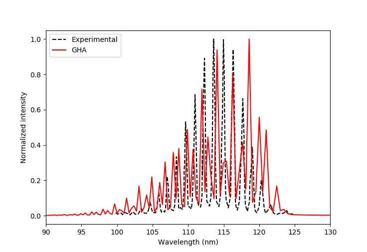
Figure 1: Photoelectron spectra of ammonia. The full red line corresponds to the theoretical simulation obtained with the GHA. The dashed black line is the experimental spectrum.[51]

As evident from Fig. 1, the GHA poorly predicts the photoelectron spectra of ammonia. The simulated spectrum is broader than experimental one, and the vibrational progressions do not match. While the experimental spectrum has an envelope that is more or less symmetric with an even distribution of peak intensities, the GHA counterpart is highly asymmetric and peaks do not seem to follow a particular pattern. Peak spacings are also incorrect in the GHA spectrum—they are much closer together than in the experiment, implying more Franck-Condon transitions than there should be. The failures of the GHA have been documented in many studies [52, 53, 17, 18].

III.2.2 The $\Delta$-KRR scheme and reducing the dimensionality of the training set

As can be seen in Fig. 2, $\Delta$-KRR-simulated spectrum agrees very well with the experimental one. The anharmonic model correctly reproduces the spacings between the peaks. It captures the relative intensities much better than the GHA, albeit with some peaks having slightly smaller amplitudes than their experimental counterpart. Overall, it is considerable improvement over the GHA.

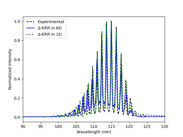
Figure 2: Photoelectron spectra of ammonia. The full blue line corresponds to the theoretical simulation obtained with an anharmonic corrective $\Delta$-KRR-fitted potential sampling all six CVMs. The green dotted line corresponds to the theoretical simulation obtained with an anharmonic corrective $\Delta$-KRR-fitted potential in which the training set samples the nuclear configurational space across two CVMs. The experimental spectrum is taken from Ref. 51. The theoretical spectra were shifted to the left by 2.0 and 1.8 nm, respectively.

The nuclear geometry of the minima of NH3 projected onto the vibrational normal modes of NH3+ can be represented by the array

$$\begin{bmatrix}48.52&-0.10&-0.21&11.71&0.42&-0.73\end{bmatrix}.$$ (28)

The two largest coefficients, 48.52 and 11.71, correspond to nuclear displacements along the pyramidal inversion and symmetric N-H bond stretching modes, respectively. Being two orders of magnitudes larger than the other contribution suggests that the only relevant anharmonic displacements are those in the subspace spanned by these two modes.

Our sampling scheme can be readily adapted to cases when only a few nuclear degrees of freedom (DOF) are strongly anharmonic. Rather than sampling all CVMs for the training set evenly, it might be beneficial to put more weight on strongly anharmonic ones. To confirm this expectation, we trained another $\Delta$-KRR model, this time involving the first and the fourth CVMs, and the couplings between them when generating the training set. This reduced-dimensionality $\Delta$-KRR model effectively samples nuclear configurations predominantly in a subspace spanned by the CVMs corresponding to the pyramidal inversion and the symmetric bond stretch modes, and trains the anharmonic corrections from there. Nevertheless, the reduced model still maps the nuclear geometry represented in all six dimensions only giving more weight to the large-amplitude modes, such that the GWP dynamics are still performed in the 6D vibrational space.

Figure 2 displays the photoelectron spectrum obtained using a reduced $\Delta$-KRR model. The methodology used to train the reduced model was the same as the full 6D one. The reduced model demonstrates a great improvement over the GHA. It captures the peaks spacings almost perfectly and their amplitudes are reproduced even better than in the full 6D model. Both models were trained using 2000 nuclear configurations sampled from perturbed CVMs scans. However, while these were scattered among six dimensions in the full $\Delta$-KRR model, in the reduced model they are distributed much more densely in a lower-dimensional space. As a result, the fitting quality is higher resulting in a better spectrum.

III.2.3 The KRR scheme for learning the entire PES

As was mentioned previously, a standard approach to construction of ML-PESs is to fit electronic energies rather than anharmonic corrections. Hence, an obvious concern is whether the $\Delta$-KRR scheme is superior to its KRR counterpart. To answer this question, we simulated the photoelectron spectra using a KRR model trained to reproduce the electronic energies rather than anharmonic corrections. To this end, we removed $v_{h}^{g}$ from Eq. (7) and $V_{h}(\bm{R}_{j})$ from Eq. (22a).

First, we considered a training set of approximately the same size as that for the $\Delta$-KRR scheme, with 2023 elements. As can be seen in Fig. 3, although the corresponding simulation captured the envelope of the spectra, it failed to demonstrate vibration progressions due to extremely poor resolution, despite having a %MAER of 97.4%. Suspecting that the KRR scheme requires a larger training set, we retrained the KRR model with a training set with 4732 elements, essentially doubling the size. As can be seen in Fig. 3, the corresponding theoretical spectrum is much closer to the experimental counterpart, representing a great improvement over the one provided by the KRR model trained with a smaller training set. However, despite the increased computational efforts needed to train the KRR model, its spectrum remains slightly inferior to the ones obtained with the $\Delta$-KRR models.

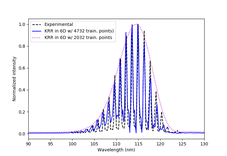
Figure 3: Photoelectron spectra of ammonia. The magenta dotted line corresponds to the theoretical simulation obtained by fiting the electronic energies with 2032 training points and the blue line with 4732 training points. The experimental spectrum is taken from Ref. 51. The theoretical spectra were translated to the left by 1.5 and 2.1 nm, respectively.

The limitations of the KRR model trained on the smaller, training set of 2023 elements became more evident when the dynamics of the center of the wavepacket were visualized. Upon leaving the Franck-Condon region, the distances between the nitrogen and each of the hydrogens atoms started growing steadily and without bounds leading to complete molecular dissociation. It is clear that the wavepacket left the properly sampled region of the PES and evolved on a nuclear potential that was effectively flat. By sampling the nuclear configurational space more thoroughly with 4732 elements, the PES was better represented, which prevented dissociation.

Both KRR and $\Delta$-KRR values can be interpreted as corrections to some reference potential. In the case of KRR, this reference potential is a flat 6D surface. The KRR model improves this flat potential by adding a Gaussian function at the location of each element of the training set. With insufficient sampling certain parts of the PES remain flat. Thus, when the GWP reaches these regions, its dynamics resembles thoses occuring on a flat potential. In the case of the $\Delta$-KRR model, the reference potential is a 6D paraboloid. If the wavepacket reaches a region that has not been sampled adequately, it will still experience a bound potential preventing dissociative nuclear dynamics.

IV Conclusions

In this study, we examined the propagation of a single thawed Gaussian wavepacket on a harmonic PES with KRR-fitted anharmonic corrections. The KRR scheme relies upon the Gaussian kernel, which complements nicely the wave function form, allowing for analytic evaluation of anharmonic terms.

This type of $\Delta$-ML approach to PES fitting was tested on the nuclear dynamics responsible for the photoelectron spectrum of ammonia. We found that the quality of the simulated spectrum is vastly superior to that of predicted with the use of global harmonic approximation and compares very favorably to the experimental results. The $\Delta$-KRR simulations predict the correct spacings and intensities of the vibrational progressions.

We also compared the $\Delta$-KRR approach to the standard one, which consists of fiting the total electronic energies. We have shown that while it is possible to reproduce the photoelectron spectrum of ammonia, albeit not as well as the $\Delta$-KRR approach, larger training sets are required.

This study also highlights the importance of selecting relevant nuclear configurations to generate small but functional ML training sets. We examined an approach that considers a simplified rigid-rotor model of a molecule to sample “soft” nuclear DOF responsible for the large-amplitude motions, such as bend and torsion angles. By running classical dynamics simulations of this model, initiated along the normal modes, we identified the regions of the nuclear configuration space that are expected to provide large anharmonic corrections to the reference harmonic potential. Additionally, this sampling approach allowed us to construct a reduced-dimensionality scheme, in which only a priori strongly anharmonic modes are needed to be sampled. Photoelectron spectra simulations of ammonia confirmed the viability of our approach, but its full potential is a subject of future studies.

Appendix A The Dirac–Frenkel variational principle

The Dirac–Frenkel variational principle (DFVP) [35, 36, 37] can be used to approximate quantum dynamics when the wavefunction $\chi(\mathbf{R},t)$ is constrained to a parametric form. The parametric EOM are found by solving

$$\matrixelement{\delta\chi}{\hat{H}-i\frac{d}{dt}}{\chi}=0,$$ (29)

where $\chi(\mathbf{R},t)$ is defined at all times through parameters $\bm{\lambda}(t)$ that evolve in time, $\chi(\mathbf{R},t)\rightarrow\chi(\mathbf{R}|\bm{\lambda}(t))$. In cases where there are a finite number of parameters, $\bm{\lambda}$ is a 1D array that contains the parameters that define the wavefunction. Using the chain rule, the variation $\delta\chi$ and the time-derivative $\frac{d\chi}{dt}$ can be expressed as

$$\delta\chi=\sum_{j}\frac{\partial\chi}{\partial\lambda_{j}}\delta\lambda_{j},$$ (30a)

$$\frac{d\chi}{dt}=\sum_{j}\frac{\partial\chi}{\partial\lambda_{j}}\frac{d\lambda_{j}}{dt}.$$ (30b)

By plugging these expressions into Eq. (29), we obtain

$$\left\langle{\frac{\partial\chi}{\partial\lambda_{j}}}\middle|{\hat{H}}\middle|{\chi}\right\rangle=i\sum_{jk}\left\langle{\frac{\partial\chi}{\partial\lambda_{j}}}\middle|{\frac{\partial\chi}{\partial\lambda_{k}}}\right\rangle\frac{d\lambda_{k}}{dt},$$ (31)

which can be rewritten in the matrix form,

$$\bm{h}=i\bm{\check{M}}\frac{d\bm{\lambda}}{dt},$$ (32)

where $h_{j}=\left\langle\frac{\partial\chi}{\partial\lambda_{j}}\middle|\hat{H}\middle|\chi\right\rangle$ and $M_{jk}=\left\langle\frac{\partial\chi}{\partial\lambda_{j}}\middle|\frac{\partial\chi}{\partial\lambda_{k}}\right\rangle$. Quantum dynamics can then be approximated by evaluating $\bm{h}$ and $\bm{\check{M}}$ and integrating Eq. (32). For a thawed Gaussian ansatz, Eq. (30) becomes

$$\delta\chi =\sum_{jk}\frac{\partial\chi}{\partial\sigma_{jk}}\delta\sigma_{jk}+\sum_{j}\frac{{\partial\chi}}{\partial P_{j}}\delta P_{l}+\frac{\partial\chi}{\partial\gamma}\delta\gamma,$$ (33)

$$\frac{d\chi}{dt} =\sum_{jk}\frac{\partial\chi}{\partial\sigma_{jk}}\frac{d\sigma_{jk}}{dt}+\sum_{j}\frac{{\partial\chi}}{\partial P_{j}}\frac{dP_{j}}{dt}+\frac{\partial\chi}{\partial\gamma}\frac{d\gamma}{dt},$$ (34)

and Eq. (32) becomes Eq. (4).

Appendix B Moments of the nuclear density

Computation of $\bm{h^{g}}$ and $\bm{\check{M}}^{\bm{g}}$ reduces to computing all moments up to fourth order of the nuclear density. Zeroth, first, second, third and fourth-order moments of the nuclear density are hereon denoted as ${m^{(0)}}$, $\bm{m}^{(1)}$, $\bm{\check{m}}^{(2)}$, $\bm{m}^{(3)}$ and $\bm{m}^{(4)}$, respectively. With the exception of ${m}^{(0)}$, which is a scalar quantity, the moments are arrays whose elements are the multidimensional integrals

$${m}^{(0)}=\int_{-\infty}^{\infty}\rho(\bm{R})d\bm{R},\\$$ (35a)

$${m}_{j}^{(1)}=\int_{-\infty}^{\infty}R_{j}\rho(\bm{R})d\bm{R},\\$$ (35b)

$${m}_{jk}^{(2)}=\int_{-\infty}^{\infty}R_{j}R_{k}\rho(\bm{R})d\bm{R},\\$$ (35c)

$${m}_{jkl}^{(3)}=\int_{-\infty}^{\infty}R_{j}R_{k}R_{l}\rho(\bm{R})d\bm{R},$$ (35d)

$${m}_{jkln}^{(4)}=\int_{-\infty}^{\infty}R_{j}R_{k}R_{l}R_{n}\rho(\bm{R})d\bm{R},$$ (35e)

where $R_{j}$, $R_{k}$, $R_{l}$ and $R_{n}$ are nuclear degrees of freedom, and $\rho(\bm{R})=\chi^{*}(\bm{R})\chi(\bm{R})$.

The moments correspond to the derivatives of a multidimensional generating function $G(\bm{\tau})=\int\exp(\bm{\tau}^{\intercal}\bm{R})\rho(\bm{R})d\bm{R}$. By Taylor expanding $\exp(\bm{\tau}^{\intercal}\bm{R})$

$$G(\bm{\tau}) =\int_{-\infty}^{+\infty}\rho(\bm{R})d\bm{R}+\sum_{k}\tau_{k}\int_{-\infty}^{+\infty}R_{k}\rho(\bm{R})d\bm{R}$$ (36)

$$+\frac{1}{2!}\sum_{kl}\tau_{k}\tau_{l}\int_{-\infty}^{+\infty}R_{k}R_{l}\rho(\bm{R})d\bm{R}+\cdots$$

$$={m}^{(0)}+\sum_{j}\tau_{j}{m}_{j}^{(1)}+\frac{1}{2!}\sum_{jk}\tau_{j}\tau_{k}{m}_{jk}^{(2)}+\cdots$$

it becomes clear that the moments correspond to the partial derivatives of $G(\bm{\tau})$ with respect to $\bm{\tau}$. Since the wavepacket is a Gaussian, $G(\bm{\tau})$ is also a Gaussian

$$G(\bm{\Gamma})=\beta\exp\left(\bm{\Gamma}^{\intercal}\bm{\check{\alpha}}\bm{\Gamma}\right),$$ (37)

where

$$\beta=N^{2}\exp(\gamma_{r})\sqrt{\frac{\pi^{d}}{\det(\bm{\check{\sigma}_{r}})}},$$ (38a)

$$\bm{\check{\alpha}}=\frac{\bm{\check{\sigma}_{r}}^{-1}}{4},$$ (38b)

$$\bm{\Gamma}=\bm{p_{r}}+\bm{\tau},$$ (38c)

where $\bm{\check{\sigma}_{r}}$ is defined in Sec. II.2. The moments can then be directly calculated

$$\begin{split}{m}_{j}^{(1)}&=\frac{\partial G(\bm{\Gamma})}{\partial\Gamma_{j}}\bigg{\rvert}_{\bm{\Gamma}=\bm{p_{r}}}\\ &=G(\bm{p_{r}}){F_{j}^{{}^{\prime}}},\end{split}$$ (39a)

$$\begin{split}{m}_{jk}^{(2)}&=\frac{\partial^{2}G(\bm{\Gamma})}{\partial\tau_{j}\partial\tau_{k}}\bigg{\rvert}_{\bm{\Gamma}=\bm{p_{r}}}\\ &=G(\bm{p_{r}})\left(F_{j}^{{}^{\prime}}F_{k}^{{}^{\prime}}+F_{jk}^{{}^{\prime\prime}}\right),\end{split}$$ (39b)

$$\begin{split}{m}_{jkl}^{(3)}&=\frac{\partial^{3}G(\bm{\Gamma})}{\partial\tau_{j}\partial\tau_{k}\partial\tau_{l}}\bigg{\rvert}_{\bm{\Gamma}=\bm{p_{r}}}\\ &=G(\bm{p_{r}})\left(F_{j}^{{}^{\prime}}F_{k}^{{}^{\prime}}F_{l}^{{}^{\prime}}+F_{jk}^{{}^{\prime\prime}}F_{l}^{{}^{\prime}}+F_{jl}^{{}^{\prime\prime}}F_{k}^{{}^{\prime}}+F_{kl}^{{}^{\prime\prime}}F_{j}^{{}^{\prime}}\right),\end{split}$$ (39c)

$$\begin{split}{m}_{jkln}^{(4)}&=\frac{\partial^{4}G(\bm{\Gamma})}{\partial\tau_{j}\partial\tau_{k}\partial\tau_{l}\partial\tau_{n}}\bigg{\rvert}_{\bm{\Gamma}=\bm{p_{r}}}\\ &=G(\bm{p_{r}})\Bigl{(}F_{j}^{{}^{\prime}}F_{k}^{{}^{\prime}}F_{l}^{{}^{\prime}}F_{n}^{{}^{\prime}}+F_{jk}^{{}^{\prime\prime}}F_{l}^{{}^{\prime}}F_{n}^{{}^{\prime}}+F_{jl}^{{}^{\prime\prime}}F_{k}^{{}^{\prime}}F_{n}^{{}^{\prime}}\\ &+F_{kn}^{{}^{\prime\prime}}F_{l}^{{}^{\prime}}F_{n}^{{}^{\prime}}+F_{lm}^{{}^{\prime\prime}}F_{k}^{{}^{\prime}}F_{n}^{{}^{\prime}}+F_{kn}^{{}^{\prime\prime}}F_{j}^{{}^{\prime}}F_{l}^{{}^{\prime}}\\ &+F_{ln}^{{}^{\prime\prime}}F_{j}^{{}^{\prime}}F_{k}^{{}^{\prime}}+F_{jk}^{{}^{\prime\prime}}F_{ln}^{{}^{\prime\prime}}+F_{jl}^{{}^{\prime\prime}}F_{kn}^{{}^{\prime\prime}}+F_{jn}^{{}^{\prime\prime}}F_{kl}^{{}^{\prime\prime}}\Bigr{)},\end{split}$$ (39d)

where $\bm{F^{{}^{\prime}}}=\bm{2\check{\alpha}\bm{p_{r}}}$ and $\bm{\check{F}^{{}^{\prime\prime}}=2\bm{\check{\alpha}}}$.

Appendix C Computing

The partial derivatives of the GWP with respect to its parameters are needed in order to compute $\bm{h^{g}}$ and $\bm{\check{M}^{g}}$. Since the DFVP conserves the norm of the wavefunction,[7] $\frac{\partial N}{\partial t}$ can be ignored and we only need to consider the derivatives of the exponential

$$\frac{\partial\chi(\bm{R}|\bm{\check{\sigma}},\bm{P},\gamma)}{\partial\sigma_{jj}}=-R_{j}^{2}\chi(\bm{R}|\bm{\check{\sigma}},\bm{P},\gamma),\\$$ (40a)

$$\frac{\partial\chi(\bm{R}|\bm{\check{\sigma}},\bm{P},\gamma)}{\partial\sigma_{jk}}=-2R_{j}R_{k}\chi(\bm{R}|\bm{\check{\sigma}},\bm{P},\gamma),\\$$ (40b)

$$\frac{\partial\chi(\bm{R}|\bm{\check{\sigma}},\bm{P},\gamma)}{\partial P_{j}}=R_{j}\chi(\bm{R}|\bm{\check{\sigma}},\bm{P},\gamma,),\\$$ (40c)

$$\frac{\partial\chi(\bm{R}|\bm{\check{\sigma}},\bm{P},\gamma)}{\partial\gamma}=\chi(\bm{R}|\bm{\check{\sigma}},\bm{P},\gamma).$$ (40d)

Equation (40) is obtained using the symmetric nature of $\bm{\check{\sigma}}$ that allows the exponential part of the wavepacket to be expressed as

$$\exp\left(-\sum_{j}\sigma_{jj}R_{j}^{2}-\sum_{j}\sum_{k>j}2\sigma_{jk}R_{j}R_{k}+\sum_{j}P_{j}R_{j}+\gamma\right).$$ (41)

Elements of $\bm{\check{M}^{g}}$ are readily computed from the moments of the nuclear density (see Eq. (39))

$${M}_{jkln}^{\bm{\check{\sigma}}\bm{\check{\sigma}}}=4{m}_{jkln}^{(4)},$$ (42a)

$${M}_{jjln}^{\bm{\check{\sigma}}\bm{\check{\sigma}}}=2{m}_{jjln}^{(4)},$$ (42b)

$${M}_{jkll}^{\bm{\check{\sigma}}\bm{\check{\sigma}}}=2{m}_{jkll}^{(4)},$$ (42c)

$${M}_{jjll}^{\bm{\check{\sigma}}\bm{\check{\sigma}}}={m}_{jjll}^{(4)},$$ (42d)

$${M}_{jkl}^{\bm{\check{\sigma}}\bm{P}}=-2{m}_{jkl}^{(3)},$$ (42e)

$${M}_{jjl}^{\bm{\check{\sigma}}\bm{P}}=-{m}_{jjl}^{(3)},$$ (42f)

$${M}_{jk}^{\bm{\check{\sigma}}\gamma}=-2{m}_{jk}^{(2)},$$ (42g)

$${M}_{jj}^{\bm{\check{\sigma}}\gamma}=-{m}_{jj}^{(2)},$$ (42h)

$${M}_{jk}^{\bm{P}\bm{P}}={m}_{jk}^{(2)},$$ (42i)

$${M}_{j}^{\bm{P}\gamma}={m}_{j}^{(1)},$$ (42j)

$${M}^{\gamma\gamma}=1.$$ (42k)

The computation of $\bm{h^{g}}$ is more involved. The kinetic energy term $\left|\hat{T}\chi\right\rangle$ requires computing the action of the Laplacian on the wavepacket

$$\begin{split}\frac{\partial^{2}\chi(\bm{R})}{\partial R_{j}}&=\chi(\bm{R})\Biggl{(}4\sigma_{jj}^{2}R_{j}^{2}-4\sigma_{jj}P_{j}R_{j}-2\sigma_{jj}+P_{j}^{2}-\sum_{k\neq j}4\sigma_{jk}P_{j}R_{k}\\ &+\sum_{k\neq j}8\sigma_{jj}\sigma_{jk}R_{j}R_{k}+\sum_{k\neq j}\sum_{l\neq j}4\sigma_{jk}\sigma_{jl}R_{k}R_{l}\Biggl{)}.\end{split}$$ (43)

The components of $\bm{t^{g}}$ are weighted sums of different moments of the nuclear density

$$\begin{split}\left\langle\frac{\partial\chi}{\partial\sigma_{mn}}\middle|\hat{T}\chi\right\rangle&=\sum_{j}\Biggl{(}4\sigma_{jj}^{2}m_{mnjj}^{(4)}-4\sigma_{jj}P_{k}m_{mnj}^{(3)}-2\sigma_{jj}m_{mn}^{(2)}+P_{j}^{2}m_{mn}^{(2)}-\sum_{l\neq j}4\sigma_{jl}P_{j}m_{mnl}^{(3)}\\ &+\sum_{l\neq j}8\sigma_{jj}\sigma_{jl}m_{mnlj}^{(4)}+\sum_{k\neq j}\sum_{l\neq j}4\sigma_{jl}\sigma_{jk}m_{mnkl}^{(4)}\Biggr{)},\end{split}$$ (44a)

$$\begin{split}\left\langle\frac{\partial\chi}{\partial\sigma_{nn}}\middle|\hat{T}\chi\right\rangle&=\frac{1}{2}\sum_{j}\Biggl{(}4\sigma_{jj}^{2}m_{nnjj}^{(4)}-4\sigma_{jj}P_{k}m_{nnj}^{(3)}-2\sigma_{jj}m_{nn}^{(2)}+P_{k}^{2}m_{nn}^{(2)}-\sum_{l\neq j}4\sigma_{jl}P_{j}m_{nnl}^{(3)}\\ &+\sum_{l\neq j}8\sigma_{jj}\sigma_{jl}m_{nnlj}^{(4)}+\sum_{k\neq j}\sum_{l\neq j}4\sigma_{jl}\sigma_{jk}m_{nnkl}^{(4)}\Biggr{)},\end{split}$$ (44b)

$$\begin{split}\left\langle\frac{\partial\chi}{\partial P_{n}}\middle|\hat{T}\chi\right\rangle&=-\frac{1}{2}\sum_{j}\Biggl{(}4\sigma_{jj}^{2}m_{njj}^{(3)}-4\sigma_{jj}P_{k}m_{nj}^{(2)}-2\sigma_{jj}m_{n}^{(1)}+P_{j}^{2}m_{n}^{(1)}-\sum_{l\neq j}4\sigma_{jl}P_{k}m_{nl}^{(2)}\\ &+\sum_{l\neq j}8\sigma_{jj}\sigma_{jl}m_{nlj}^{(3)}+\sum_{k\neq j}\sum_{l\neq j}4\sigma_{jl}\sigma_{jk}m_{nkl}^{(3)}\Biggr{)},\end{split}$$ (44c)

$$\begin{split}\left\langle\frac{\partial\chi}{\partial\gamma}\middle|\hat{T}\chi\right\rangle&=-\frac{1}{2}\sum_{j}\Biggl{(}4\sigma_{jj}^{2}m_{jj}^{(2)}-4\sigma_{jj}P_{k}m_{j}^{(1)}-2\sigma_{jj}+P_{j}^{2}-\sum_{l\neq j}4\sigma_{jl}P_{j}m_{l}^{(1)}\\ &+\sum_{l\neq j}8\sigma_{jj}\sigma_{jl}m_{lj}^{(2)}+\sum_{k\neq j}\sum_{l\neq j}4\sigma_{jl}\sigma_{jk}m_{kl}^{(2)}\Biggr{)},\end{split}$$ (44d)

while the components of $\bm{v}_{h}^{g}$ are

$$\left\langle\frac{\partial\chi}{\partial\sigma_{nn}}\middle|\hat{V}_{h}\chi\right\rangle=-\frac{1}{2}\sum_{j}\omega_{j}^{2}m_{nnjj}^{(4)},$$ (45a)

$$\left\langle\frac{\partial\chi}{\partial\sigma_{mn}}\middle|\hat{V}_{h}\chi\right\rangle=-\sum_{j}\omega_{j}^{2}m_{mnjj}^{(4)},$$ (45b)

$$\left\langle\frac{\partial\chi}{\partial P_{n}}\middle|\hat{V}_{h}\chi\right\rangle=\frac{1}{2}\sum_{j}\omega_{j}^{2}m_{njj}^{(3)},$$ (45c)

$$\left\langle\frac{\partial\chi}{\partial\gamma}\middle|\hat{V}_{h}\chi\right\rangle=\frac{1}{2}\sum_{j}\omega_{j}^{2}m_{jj}^{(2)}.$$ (45d)

References

- Heller [1981] E. J. Heller, “The semiclassical way to molecular spectroscopy,” Acc. Chem. Res. 14, 368–375 (1981).
- Tannor [2007] D. J. Tannor, Introduction to Quantum Mechanics: a Time-Dependent Perspective (University Science Books, Sausalito, CA, USA, 2007) p. 437.
- Niu et al. [2010] Y. Niu, Q. Peng, C. Deng, X. Gao, and Z. Shuai, “Theory of excited state decays and optical spectra: Application to polyatomic molecules,” J. Phys. Chem. A 114, 7817–7831 (2010).
- Peng et al. [2010] Q. Peng, Y. Niu, C. Deng, and Z. Shuai, “Vibration correlation function formalism of radiative and non-radiative rates for complex molecules,” Chem. Phys. 370, 215–222 (2010).
- Baiardi, Bloino, and Barone [2013] A. Baiardi, J. Bloino, and V. Barone, “General time dependent approach to vibronic spectroscopy including franck–condon, herzberg–teller, and duschinsky effects,” J. Chem. Theory Comput. 9, 4097–4115 (2013).
- Kosloff [1988] R. Kosloff, “Time-dependent quantum-mechanical methods for molecular dynamics,” J. Phys. Chem. 92, 2087–2100 (1988).
- [7] H. Meyer, “Introduction to mctdh,” ttps://www.pci.uni-heidelberg.de/tc/usr/mctdh/lit/intro_MCTDH.pdf, accessed: 2023-03-30.
- Beck et al. [2000] M. H. Beck, A. Jäckle, G. A. Worth, and H.-D. Meyer, “The multiconfiguration time-dependent hartree (mctdh) method: a highly efficient algorithm for propagating wavepackets,” Phys. Rep. 324, 1–105 (2000).
- Sawada and Metiu [1986] S.-I. Sawada and H. Metiu, “A gaussian wave packet method for studying time dependent quantum mechanics in a curve crossing system: Low energy motion, tunneling, and thermal dissipation,” J. Chem. Phys. 84, 6293–6311 (1986).
- Worth, Robb, and Burghardt [2004] G. A. Worth, M. A. Robb, and I. Burghardt, “A novel algorithm for non-adiabatic direct dynamics using variational gaussian wavepackets,” Faraday Discuss. 127, 307–323 (2004).
- Curchod and Martínez [2018] B. F. Curchod and T. J. Martínez, “Ab initio nonadiabatic quantum molecular dynamics,” Chem. Rev. 118, 3305–3336 (2018).
- Worth and Lasorne [2020] G. A. Worth and B. Lasorne, “Gaussian wave packets and the dd-vmcg approach,” Quantum Chemistry and Dynamics of Excited States: Methods and Applications , 413–433 (2020).
- Joubert-Doriol [2022] L. Joubert-Doriol, “Variational approach for linearly dependent moving bases in quantum dynamics: application to gaussian functions,” J. Chem. Theory Comput. 18, 5799–5809 (2022).
- JL Vaníček [2023] J. JL Vaníček, “Family of gaussian wavepacket dynamics methods from the perspective of a nonlinear schrödinger equation,” J. Chem. Phys. 159 (2023).
- Richings et al. [2015] G. W. Richings, I. Polyak, K. E. Spinlove, G. A. Worth, I. Burghardt, and B. Lasorne, “Quantum dynamics simulations using gaussian wavepackets: the vmcg method,” Int. Rev. Phys. Chem. 34, 269–308 (2015).
- Ben-Nun and Martinez [2000] M. Ben-Nun and T. J. Martinez, “A multiple spawning approach to tunneling dynamics,” J. Chem. Phys. 112, 6113–6121 (2000).
- Wehrle, Oberli, and Vanicek [2015] M. Wehrle, S. Oberli, and J. Vanicek, “On-the-fly ab initio semiclassical dynamics of floppy molecules: Absorption and photoelectron spectra of ammonia,” J. Phys. Chem. A 119, 5685–5690 (2015).
- Begusic, Tapavicza, and Vanicek [2022] T. Begusic, E. Tapavicza, and J. Vanicek, “Applicability of the thawed gaussian wavepacket dynamics to the calculation of vibronic spectra of molecules with double-well potential energy surfaces,” J. Chem. Theory Comput. 18, 3065–3074 (2022).
- Heller [1975] E. J. Heller, “Time-dependent approach to semiclassical dynamics,” J. Chem. Phys. 62, 1544–1555 (1975).
- Frankcombe, Collins, and Worth [2010] T. J. Frankcombe, M. A. Collins, and G. A. Worth, “Converged quantum dynamics with modified shepard interpolation and gaussian wave packets,” Chem. Phys. Lett. 489, 242–247 (2010).
- Polyak et al. [2019] I. Polyak, G. W. Richings, S. Habershon, and P. J. Knowles, “Direct quantum dynamics using variational gaussian wavepackets and gaussian process regression,” J. Chem. Phys. 150, 041101 (2019).
- Alborzpour, Tew, and Habershon [2016] J. P. Alborzpour, D. P. Tew, and S. Habershon, “Efficient and accurate evaluation of potential energy matrix elements for quantum dynamics using gaussian process regression,” J. Chem. Phys. 145, 174112 (2016).
- Richings and Habershon [2017] G. W. Richings and S. Habershon, “Direct quantum dynamics using grid-based wave function propagation and machine-learned potential energy surfaces,” J. Chem. Theory Comput. 13, 4012–4024 (2017).
- Koch et al. [2019] W. Koch, M. Bonfanti, P. Eisenbrandt, A. Nandi, B. Fu, J. Bowman, D. Tannor, and I. Burghardt, “Two-layer gaussian-based mctdh study of the s 1← s 0 vibronic absorption spectrum of formaldehyde using multiplicative neural network potentials,” J. Chem. Phys. 151, 064121 (2019).
- Ramakrishnan et al. [2015a] R. Ramakrishnan, P. O. Dral, M. Rupp, and O. A. Von Lilienfeld, “Big data meets quantum chemistry approximations: the -machine learning approach,” J. Chem. Theory Comput. 11, 2087–2096 (2015a).
- Ramakrishnan et al. [2015b] R. Ramakrishnan, M. Hartmann, E. Tapavicza, and O. A. Von Lilienfeld, “Electronic spectra from tddft and machine learning in chemical space,” J. Chem. Phys. 143 (2015b).
- Ruth, Gerbig, and Schreiner [2022] M. Ruth, D. Gerbig, and P. R. Schreiner, “Machine learning of coupled cluster (t)-energy corrections via delta ()-learning,” J. Chem. Theory Comput. 18, 4846–4855 (2022).
- Vovk [2013] V. Vovk, “Kernel ridge regression,” Empirical Inference: Festschrift in Honor of Vladimir N. Vapnik , 105–116 (2013).
- Unke and Meuwly [2017] O. T. Unke and M. Meuwly, “Toolkit for the construction of reproducing kernel-based representations of data: Application to multidimensional potential energy surfaces,” J. Chem. Inf. Model. 57, 1923–1931 (2017).
- Dral et al. [2017] P. O. Dral, A. Owens, S. N. Yurchenko, and W. Thiel, “Structure-based sampling and self-correcting machine learning for accurate calculations of potential energy surfaces and vibrational levels,” J. Chem. Phys. 146, 244108 (2017), https://doi.org/10.1063/1.4989536 .
- Hu et al. [2018] D. Hu, Y. Xie, X. Li, L. Li, and Z. Lan, “Inclusion of machine learning kernel ridge regression potential energy surfaces in on-the-fly nonadiabatic molecular dynamics simulation,” J. Phys. Chem. Let. 9, 2725–2732 (2018).
- Westermayr et al. [2020] J. Westermayr, F. A. Faber, A. S. Christensen, O. A. von Lilienfeld, and P. Marquetand, “Neural networks and kernel ridge regression for excited states dynamics of ch2nh: From single-state to multi-state representations and multi-property machine learning models,” Mach. Learn.: Sci. Technol. 1, 025009 (2020).
- Dral [2020] P. O. Dral, “Quantum chemistry assisted by machine learning,” in Adv. Quantum Chem., Vol. 81 (Elsevier, 2020) pp. 291–324.
- Pinheiro et al. [2021] M. Pinheiro, F. Ge, N. Ferré, P. O. Dral, and M. Barbatti, “Choosing the right molecular machine learning potential,” Chem. Sci. 12, 14396–14413 (2021).
- Dirac [1930] P. A. Dirac, “Note on exchange phenomena in the thomas atom,” in Math. Proc. Camb. Philos. Soc., Vol. 26 (Cambridge University Press, 1930) pp. 376–385.
- Frenkel et al. [1934] J. Frenkel et al., Wave mechanics, advanced general theory, Vol. 436 (Oxford, 1934).
- McLachlan [1964] A. McLachlan, “A variational solution of the time-dependent schrodinger equation,” Mol. Phys. 8, 39–44 (1964).
- Vaidehi and Jain [2015] N. Vaidehi and A. Jain, “Internal coordinate molecular dynamics: A foundation for multiscale dynamics,” J. Phys. Chem. B 119, 1233–1242 (2015).
- Marsili et al. [2022] E. Marsili, F. Agostini, A. Nauts, and D. Lauvergnat, “Quantum dynamics with curvilinear coordinates: models and kinetic energy operator,” Philos. Trans. Royal Soc. A 380, 20200388 (2022).
- Vendrell et al. [2007] O. Vendrell, F. Gatti, D. Lauvergnat, and H.-D. Meyer, “Full-dimensional (15-dimensional) quantum-dynamical simulation of the protonated water dimer. i. hamiltonian setup and analysis of the ground vibrational state,” J. Chem. Phys. 127, 184302 (2007).
- Schiffel and Manthe [2010] G. Schiffel and U. Manthe, “Quantum dynamics of the h+ ch 4→ h 2+ ch 3 reaction in curvilinear coordinates: Full-dimensional and reduced dimensional calculations of reaction rates,” J. Chem. Phys. 132, 084103 (2010).
- Joubert-Doriol et al. [2012] L. Joubert-Doriol, B. Lasorne, F. Gatti, M. Schröder, O. Vendrell, and H.-D. Meyer, “Suitable coordinates for quantum dynamics: Applications using the multiconfiguration time-dependent hartree (mctdh) algorithm,” Comput. Theor. Chem. 990, 75–89 (2012).
- Becke [1993] A. D. Becke, “A new mixing of hartree–fock and local density-functional theories,” J. Chem. Phys. 98, 1372–1377 (1993).
- Lee, Yang, and Parr [1988] C. Lee, W. Yang, and R. G. Parr, “Development of the colle-salvetti correlation-energy formula into a functional of the electron density,” Phys. Rev. B 37, 785 (1988).
- Krishnan et al. [1980] R. Krishnan, J. S. Binkley, R. Seeger, and J. A. Pople, “Self-consistent molecular orbital methods. xx. a basis set for correlated wave functions,” J. Chem. Phys. 72, 650–654 (1980).
- [46] A. A. Granovsky, “Firefly version 8,” http://classic.chem.msu.su/gran/firefly/index.html, accessed: 2023-03-03.
- Butcher [2008] J. Butcher, Numerical methods for ordinary differential equations (John Wiley & Sons, 2008) pp. 109–110.
- McKay, Beckman, and Conover [2000] M. D. McKay, R. J. Beckman, and W. J. Conover, “A comparison of three methods for selecting values of input variables in the analysis of output from a computer code,” Technometrics 42, 55–61 (2000).
- An, Liu, and Venkatesh [2007] S. An, W. Liu, and S. Venkatesh, “Fast cross-validation algorithms for least squares support vector machine and kernel ridge regression,” Pattern Recognit. 40, 2154–2162 (2007).
- Smith and Warsop [1968] W. Smith and P. Warsop, “Franck-condon principle and large change of shape in polyatomic molecules,” Trans. Faraday Soc. 64, 1165–1173 (1968).
- Rabalais et al. [1973] J. Rabalais, L. Karlsson, L. Werme, T. Bergmark, and K. Siegbahn, “Analysis of vibrational structure and jahn-teller effects in the electron spectrum of ammonia,” J. Chem. Phys. 58, 3370–3372 (1973).
- Domcke et al. [1977] W. Domcke, L. Cederbaum, H. Köppel, and W. Von Niessen, “A comparison of different approaches to the calculation of franck-condon factors for polyatomic molecules,” Mol. Phys. 34, 1759–1770 (1977).
- Peluso, Borrelli, and Capobianco [2009] A. Peluso, R. Borrelli, and A. Capobianco, “Photoelectron spectrum of ammonia, a test case for the calculation of franck- condon factors in molecules undergoing large geometrical displacements upon photoionization,” J. Phys. Chem. A 113, 14831–14837 (2009).