Distribution of lowest eigenvalue in -body bosonic random matrix ensembles
Abstract
We numerically study the distribution of the lowest eigenvalue of finite many-boson systems with -body interactions modeled by Bosonic Embedded Gaussian Orthogonal [BEGOE()] and Unitary [BEGUE()] random matrix Ensembles. Following the recently established result that the -normal describes the smooth form of the eigenvalue density of the -body embedded ensembles, the first four moments of the distribution of lowest eigenvalues have been analyzed as a function of the parameter, with for and for ; being the number of bosons. Our results show the distribution exhibits a smooth transition from Gaussian like for close to 1 to a modified Gumbel like for intermediate values of to the well-known Tracy-Widom distribution for .
I Introduction
Extreme value statistics (EVS) is related to, for example, the statistics of either the lowest few or largest few eigenvalues of a matrix and has found varied applications [1, 2, 3]. Depending on the parent distribution, the classical EVS are classified into Fréchet, Gumbel and Weibull distributions [4, 5]. The classical EVS deals with the statistics of minimum or maximum of a set of random variables with a given parent distribution whereas in most of the real physical systems, the underlying variables are correlated [6]. Complex systems are usually modeled by classical random matrix ensembles - Gaussian Orthogonal (GOE), Unitary (GUE) and symplectic (GSE) Ensembles [7, 8]. The eigenvalues are correlated for these ensembles and the EVS of the (lowest) largest eigenvalues is described by the celebrated (reflected) Tracy-Widom (TW) distribution [9, 10, 11]. For a variety of random matrix ensembles, EVS has been investigated. However, one class of ensembles where there has been very little attention are embedded random matrix ensembles with -body interactions which are now established to be essential while dealing with dynamics of complex quantum many-body systems [12, 13, 14, 15, 16].
Embedded ensembles are random matrix ensembles that describe the generic properties of many-particle (fermion/boson) interacting complex systems [15]. Given number of fermions or bosons distributed in single particle levels interacting via -body interactions (), the -body fermionic or bosonic embedded ensembles are constructed by defining the -particle Hamiltonian to be a GOE (or a GUE) and then propagating it to -particle spaces using the underlying Lie algebra [15]. The case when rank of interactions equals number of fermions or bosons , we have a GOE (or a GUE). As the -particle Hamiltonian is embedded in the -particle Hamiltonian, the many-particle matrix elements are correlated for embedded ensembles (EE), unlike a GOE (or a GUE). Note that although the matrix elements for GOE (or a GUE) are independent and identically distributed random variables, its eigenvalues are correlated. Therefore, the eigenvalues of EE will have additional correlations.
Recently, numerical results for distribution of largest eigenvalue within the framework of fermionic embedded ensembles have shown a smooth transition from Gaussian to TW distribution as a function of rank of interactions [17]. In addition, for two-body fermionic and bosonic ensembles, the distribution of ground state energies was shown to follow the modified-Gumbel distribution [18]. Going further, in this paper, we focus on Bosonic Embedded Gaussian Orthogonal [BEGOE()] and Unitary [BEGUE()] random matrix Ensembles with -body interactions.
Interestingly, the transition in eigenvalue density for BEGOE() [also BEGUE()] is well described by -normal form, with parameter being related to the fourth moment of the eigenvalue density [19]. Note that, gives Gaussian eigenvalue density and this is valid for and gives semi-circle (GOE/GUE) eigenvalue density as valid for . We are interested in numerically investigating how the distribution of the lowest eigenvalues for BEGOE() [also BEGUE()] varies as a function of the parameter. For (GOE/GUE), the distribution of the lowest eigenvalues follows the well-known TW distribution [9, 10, 11].
Now, we will give a preview. Section II defines the BEGOE()/BEGUE() and gives the -normal form for the eigenvalue densities alongwith the formula for the parameter in terms of . We also give the various distributions that have been used in the present work to analyze the distribution of lowest eigenvalues. In Section III, we then analyze the first four moments of the lowest eigenvalue distribution. We compare the lowest eigenvalue distribution with EVS and study the spacing distribution between lowest eigenvalue and its nearest neighbor in Section IV. Finally, Section V gives conclusions and future outlook.
II Preliminaries
In this section, we define bosonic embedded ensembles and give the -normal form for the eigenvalue densities [19]. Then we explain the various distributions that have been used to analyze the distribution of lowest eigenvalues for BEGOE() and BEGUE().
II.1 -normal form for eigenvalue density of BEGOE()
Given a system of spin-less bosons in degenerate single particle states and say the interaction among the bosons is a -body interactions (), then the Hamiltonian operator for the system takes the form
| (1) |
Here, and denote -particle configuration states in occupation number basis and creates a normalized particle state with . Similarly is a particle annihilation operator. Note that are the matrix elements of in the defining particle space with the matrix dimension being . Here, Dyson’s parameter is equal to for GOE and for GUE. Now, representing the matrix by GOE/GUE in particle space we have a GOE/GUE ensemble of operators and action of each member of this GOE/GUE on the particle states will generate a particle matrix of dimension . The ensemble of these matrices form embedded GOE/GUE of particle interactions [BEGOE()/BEGUE() with for bosons] in particle spaces. In defining the GOE in -particle spaces, we choose the matrix elements to be independent Gaussian variables with variance 2 for diagonal matrix elements and 1 for off-diagonal matrix elements, For GUE, the variance of real and imaginary parts of the off-diagonal matrix elements are chosen to be unity.
In order to introduce the -normal form, firstly one needs the definition of numbers and they are(with ),
| (2) |
Note that . Similarly, -factorial with . Given these, the -normal distribution with being a standardized variable (then is zero centered with variance unity), is given by [20, 21]
| (3) |
The is non-zero for in the domain defined by where
| (4) |
Note that . Most important property of -normal is that is Gaussian with and similarly, , the semi-circle with .
II.2 Extreme value statistics
In the present work, we use three different distributions that characterize EVS - Classical TW distribution, modified Gumbel distribution and distribution.
II.2.1 Classical Tracy-Widom distribution
The TW distribution of lowest eigenvalues , corresponding to a -dimensional system, is given by [9, 10, 11],
| (6) |
For and 2, we have
| (7) |
where is given in terms of the solution to Painlevé type II equation subjected to the boundary condition for , with denoting the Airy function and . Note that is the Dyson’s parameter.
II.2.2 Modified Gumbel distribution
Gumbel distributions are one of the EVS and have been used to analyze ground state distribution in Sherrington-Kirkpatrick model [23] and Two-body random ensembles (TBRE) [18]. The modified Gumbel distribution is given by [4, 5],
| (8) |
with , and as functions of parameter . The provides an interpolation between the standard Gumbel () and Gaussian () distribution.
II.2.3 distribution
Lea Santos et al demonstrated that distribution (for a system with degrees of freedom) explains the distribution of lowest eigenvalues of disordered many-body quantum systems [24],
| (9) |
This distribution remains well-defined even when the free parameter is non-integer. The fitting parameter is related to skewness () as . For GOE, we have , and Eq. (9) fits TW distribution very well. Similarly, also for GUE, with and , Eq. (9) fits TW distribution very well. .
III First four moments of the lowest eigenvalue distribution
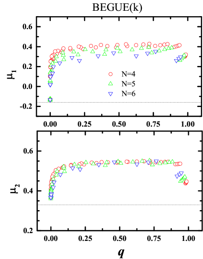
In all the examples considered in this paper, we construct a 1000 member BEGOE() and BEGUE() with following choices of number of single particle states and number of bosons : , ; , ; and , . Remember that rank of interactions takes values from 1 to . In all these examples, we obtain the lowest eigenvalue; we denote this by hereafter. For the distribution of , we will present in this Section, results for the centroid , width , skewness (defined by the third central moment) and Kurtosis (defined by the fourth central moment).
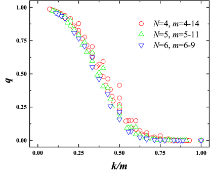
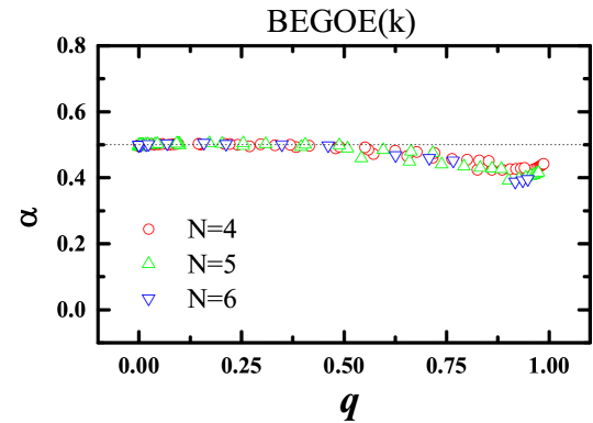
Firstly, we compute the parameter using Eq. (5) and its variation with is shown in Fig. 1. Notice the linear behavior for intermediate values of while there are strong deviations near the two extreme values of . Although the variation of with is smooth, there is very weak dependence on .
III.1 Centroid of lowest eigenvalue distribution
The -normal distribution shows that the distribution has a cut-off at at the lower edge when measured with respect to the ensemble averaged eigenvalue centroid; this follows easily from Eq. (4). For finite , there will be departures as -normal is an asymptotic form for the eigenvalue densities. Therefore, we use the following parametrization for the centroid of ’s for a given ,
| (10) |
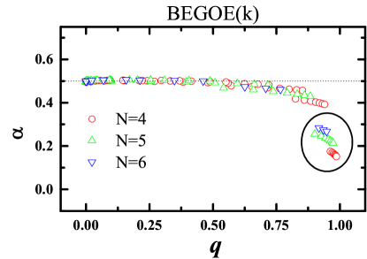
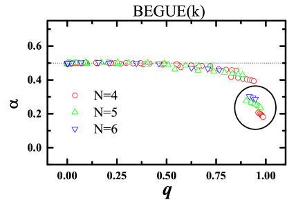
where Eq. (5) gives the formula for parameter and for BEGOE()/BEGUE(). In the limit -normal form is exact, the parameter and secondly, for , the Eq. (5) gives the well-known result for TW for GOE/GUE. Therefore, using the calculated values, via least-square procedure, we have determined the values of for all values listed above. The corresponding results are shown in Fig. 2. For , the agreement with -normal form result that is almost exact. However, for , the deviations from are significant and they correspond to . This appears to be due to the well known result that the eigenvalue centroid scaled by the spectral width fluctuations from member to member are largest for [25] and they decrease faster as increases. This also corresponds to ensemble vs spectral averaging in EE [26, 27]; see also Appendix. In addition, the systems show much larger deviations from . This is understandable as one needs atleast five single particle states for asymptotics to work well [28].
III.2 Variance of lowest eigenvalue distribution
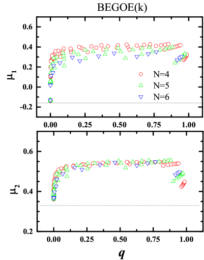
The variance for TW distribution is for -dimensional GOE/GUE. This corresponds to BEGOE()/BEGUE() with and . This is also proportional to the spectral width. Therefore, we use the following two parametrizations for bosonic EE,
| (11) |
and
| (12) |
For case, i.e. for classical Gaussian ensembles, the exponent for Eq. (11) and for Eq. (12). Both of these will give for the case .
Now, using the calculated values, via least-square procedure, we have determined the values of and for all values listed above. The results are shown in Fig. 3. For small values of , the coefficients and increase linearly and then, essentially become a constant. The values decrease for . Note that becomes positive (also increases) which implies larger variance compared to that for TW. This trend is common for both EGOE/EGUE.
 |
 |
| (a) | (b) |
III.3 Skewness and excess of lowest eigenvalue distribution
We have computed the shape parameters - skewness and kurtosis for the distribution and analyze their variation with parameter in Fig. 4 using some examples. For very small and very large values, we see departure from the linear decreasing behavior in both skewness and kurtosis. For , the value decreases from 4 to 2 while value decreases from 1.5 to 1.0. Thus, the skewness and kurtosis values are larger than those for TW distribution for intermediate values.
It might be insightful to derive the expressions for variance, skewness and kurtosis from first principles but this is beyond the scope of the present paper.
IV Lowest eigenvalue distribution: Comparison with EVS
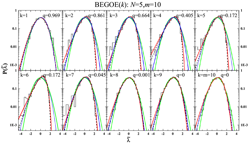
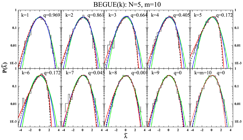
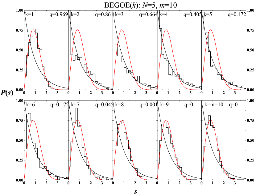
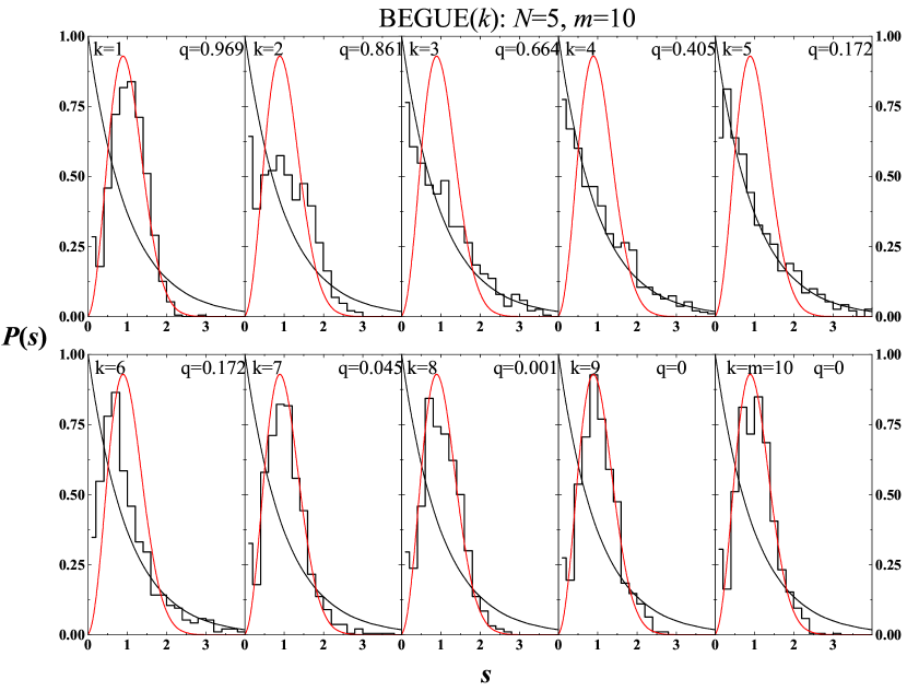
In this section, we compare the distribution of lowest eigenvalues with EVS given in Section II and also compare them to Gaussian distribution. The results for a 1000 member BEGOE() and BEGUE() are given in Figs. 5 and 6, respectively. These are obtained for and system with varying from 1 to 10. The numerical histograms are computed using the scaled lowest eigenvalues
| (13) |
We choose and system as the distributions may have smooth form only in the asymptotic limit with for bosons. Note that the modified Gumbel (smooth red curves) distributions are obtained using Eq. (8). Similarly, TW (smooth blue curves) and (black dashed curves) distributions are obtained using Eqs. (7) and (9) respectively. For , the distributions are close to Gaussian form. However, for the distributions are close to modified Gumbel form and it transitions to TW for . For BEGOE(), the values of the fitting parameter are 13(), 1.8(), 2.6(), 1.0(), 1.5(), 1.0(), 3.2(), 5.7(), 4.4() and 6.0(). Similarly, the fitting parameter for distribution are 135(), 17(), 26(), 9(), 15(), 12(), 28(), 82(), 41() and 93(). Beyond , the distributions are close to TW distributions. For BEGUE(), the values of fitting parameters and , respectively, are [12(), 4.2(), 2.8(), 2.9(), 1.5(), 1.5(), 6.2(), 7.3() 8.4(), 5.5 ()] and [136(), 34(), 28(), 24(), 14(), 14(), 97(), 145(), 69() and 160()]. Thus, the lowest eigenvalue distribution for BEGOE()/BEGUE() changes from Gaussian to modified Gumbel to Tracy-Widom as changes from () to 0 (). For fermion systems, it was concluded that there is a transition from Gaussian to TW form for the largest eigenvalue distribution [17].
Before concluding, we also studied the distribution of the spacings between lowest and the next lowest eigenvalue, which is also an extreme statistic. We use the normalized spacing which is the ratio of actual spacing with the average spacing and the results are shown in Figs. 7 and 8 respectively for BEGOE() and BEGUE(). The numerical histograms are compared with Poisson and the Wigner’s surmise results. It shows that as parameter changes, there is a transition from Wigner’s surmise to Poisson to Wigner’s surmise. An analytical derivation of this result might be valuable.
V Conclusions and future outlook
We have presented numerical results for the first four moments of the lowest eigenvalue distribution for BEGOE() and BEGUE(). We have analytical understanding of the centroid, from the -normal form of the ensemble averaged eigenvalue density for EE(k), and for the other three moments, one needs to derive analytical results. Numerical results suggest that the distribution of the lowest eigenvalues for BEGOE() and BEGUE() make a transition from Gaussian to modified Gumbel (intermediate values) to TW as we change the rank of interactions . Similarly, the distribution of normalized spacing between the lowest and next lowest eigenvalues exhibits a transition from Wigner’s surmise to Poisson to Wigner’s surmise with decreasing value. The set of numerical calculations presented in this paper for BEGOE() and BEGUE() and similarly, those in [17] for the fermionic EGOE(k) and EGUE(k) may be used may be used as a starting point for further exploring the EVS in random matrix ensembles appropriate for quantum many-body interacting systems.
Acknowledgments
M. V. acknowledges financial support from CONAHCYT project Fronteras 10872.
*
Appendix A Fluctuations in values for centroids
To further probe into the fluctuations in values from as shown in Fig. 2, we computed the parameter for each member of the ensemble using the kurtosis. Then, used along with the minimum eigenvalue for each member to calculate . Then the exponent is obtained using the equation . The results for a 1000 member BEGOE() are shown in Fig. A1. One can see that for all values, unlike as in Fig. 2. Thus, the member-to-member fluctuations in the minimum eigenvalues and parameter are giving the large deviations for from in Fig. 2. Though not shown, we expect similar results for BEGUE(). The systems with appear to be special and there are results in [29] for different types of interactions.
References
References
- [1] J. Bouchaud and M. Mézard, Universality classes for extreme-value statistics, J. Phys. A 30, 7997 (1997).
- [2] D. S. Dean and S. N. Majumdar, Extreme value statistics of eigenvalues of Gaussian random matrices, Phys. Rev. E 77, 041108 (2008).
- [3] J. Fortin and M. Clusel, Applications of extreme value statistics in physics, J. Phys. A: Mathematical and Theoretical 48, 183001 (2015).
- [4] E. J. Gumbel, Statistics of Extremes, (Columbia University Press, New York Chichester, West Sussex, 1958).
- [5] J. Galambos, The Asymptotic Theory of Extreme Order Statistics, (Malabar, FL: Krieger, 1987).
- [6] S. N. Majumdar, A. Pal and G. Schehr, Extreme value statistics of correlated random variables: A pedagogical review, Phys. Rep. 840, 1 (2020).
- [7] M.L. Mehta, Random Matrices, 3rd edition (Elsevier B.V., The Netherlands, 2004).
- [8] G. Akemann, J. Baik, and P. Di Francesco (eds.), The Oxford Handbook of Random Matrix Theory, (Oxford University Press, Oxford, 2011).
- [9] C. A. Tracy and H. Widom, Level-spacing distributions and the Airy kernel, Comm. Math. Phys. 159, 151 (1994).
- [10] C. A. Tracy and H. Widom, Level-spacing distributions and the Airy kernel, Phys. Lett. B 305, 115 (1993).
- [11] C. A. Tracy and H. Widom, On orthogonal and symplectic matrix ensembles, Comm. Math. Phys. 177, 727 (1996).
- [12] K. K. Mon and J.B. French, Statistical properties of many-particle spectra, Ann. Phys. (N.Y.) 95, 90-111 (1975).
- [13] T. A. Brody, J. Flores, J. B. French, P. A. Mello, A. Pandey, and S. S. M. Wong, Random Matrix Physics: Spectrum and Strength Fluctuations, Rev. Mod. Phys. 53, 385-479 (1981).
- [14] L. Benet and H. A. Weidenmüller, Review of the -body embedded ensembles of Gaussian random matrices, J. Phys. A 36, 3569-3594 (2003).
- [15] V. K. B. Kota, Embedded Random Matrix Ensembles in Quantum Physics, (Lecture Notes in Physics, Springer International Publishing, 2014).
- [16] Manan Vyas and T. H. Seligman, Random matrix ensembles for many-body quantum systems, AIP Conference Proceedings 1950, 030009 (2018).
- [17] E. Carro, L. Benet and I. P. Castillo, A smooth transition towards a Tracy–Widom distribution for the largest eigenvalue of interacting -body fermionic embedded Gaussian ensembles, J. Stat. Mech. 2023, 043201 (2023).
- [18] V. K. B. Kota and N. D. Chavda, Embedded random matrix ensembles from nuclear structure and their recent applications, Int. J. Mod. Phys. E 27, 1830001 (2018).
- [19] Manan Vyas and V. K. B. Kota, Quenched many-body quantum dynamics with k-body interactions using q-Hermite polynomials, J. Stat. Mech. 2019, 103103 (2019).
- [20] M. E. H. Ismail, D. Stanton and G. Viennot, The Combinatorics of -Hermite polynomials and the Askey—Wilson Integral, Eur. J. Comb. 8, 379 (1987).
- [21] P. J. Szablowski, On the -Hermite polynomials and their relationship with some other families of orthogonal polynomials, Demonstratio Math. 46, 679 (2013).
- [22] P. Rao and N.D. Chavda, Structure of wavefunction for interacting bosons in mean-field with random -body interactions, Phys. Lett. A 399, 127302 (2021).
- [23] M. Palassini, Ground-state energy fluctuations in the Sherrington–Kirkpatrick model, J. Stat. Mech. 2008, P10005 (2008).
- [24] W. Buijsman, T. Lezama, T. Leiser, and L. F. Santos, Ground-state energy distribution of disordered many-body quantum systems, Phys. Rev. E 106, 054144 (2022).
- [25] N. D. Chavda, V. Potbhare, V. K. B. Kota, Statistical properties of dense interacting boson systems with one- plus two-body random matrix ensembles, Physics Letters A 311, 331 (2003).
- [26] T. A. Brody, J. Flores, J. B. French, P. A. Mello, A. Pandey and S. S. M. Wong, Random-matrix physics: spectrum and strength fluctuations, Rev. Mod. Phys. 53, 385 (1981).
- [27] J. Flores, M. Horoi, M. Mueller and T. H. Seligman, Spectral statistics of the two-body random ensemble revisited, Phys. Rev. E 63, 026204 (2000).
- [28] K. Patel, M. S. Desai, V. Potbhare, V. K. B. Kota, Average-fluctuations separation in energy levels in dense interacting Boson systems, Physics Letters A 275, 329 (2000).
- [29] D. S. Dean, P. L. Doussal, S. N. Majumdar and G. Schehr, Noninteracting fermions at finite temperature in a -dimensional trap: Universal correlations, Phys. Rev. A 94, 063622 (2016).