Rockafellian relaxation for PDE-constrained optimization with distributional ambiguity

Abstract

Stochastic optimization problems are generally known to be ill-conditioned to the form of the underlying uncertainty. A framework is introduced for optimal control problems with partial differential equations as constraints that is robust to inaccuracies in the precise form of the problem uncertainty. The framework is based on problem relaxation and involves optimizing a bivariate, “Rockafellian” objective functional that features both a standard control variable and an additional perturbation variable that handles the distributional ambiguity. In the presence of distributional corruption, the Rockafellian objective functionals are shown in the appropriate settings to $\Gamma$-converge to uncorrupted objective functionals in the limit of vanishing corruption. Numerical examples illustrate the framework’s utility for outlier detection and removal and for variance reduction.

49M37, 90C30, 93C20, 93E20, 49K20, 49J20

1 Introduction

Many stochastic optimization problems constrained by partial differential equations (PDEs) take the form

(1) $$\min_{z\in Z_{\rm ad}}\varphi(z),\qquad\varphi(z)=f_{0}(z)+\mathbb{E}\left[g(s(\xi,z))\right]=f_{0}(z)+\int_{\Xi}g(s(\xi,z))\,d\mathbb{P}(\xi)$$

where the deterministic control variable $z$ belongs to some admissible set $Z_{\rm ad}$. Precise definitions are given below, but generally speaking, the function $s$ maps the control variable to the solution of the underlying PDE constraint, while $g$ maps the PDE solution to some quantity of interest (QoI), and $f_{0}(z)$ can be a control penalty or regularization term. As the precise form of one or more of the PDE input data may be unknown, the solution map $s$ is parameterized by some random quantity $\xi$ that belongs to a sample space $\Xi$ and follows a hypothesized distribution $\mathbb{P}$.

Problem uncertainty can arise from imprecise knowledge of the constraining PDE’s forcing terms, boundary and initial conditions, geometry, and coefficients within the differential operator, for example. In practice, the form of the uncertainty itself is often ambiguous; i.e. the sample space $\Xi$ and probability measure $\mathbb{P}$ are themselves uncertain. Typically one makes an ansatz based on empirical knowledge, which may be unsettled due to measurement error or adversarial corruption, for example.

One standard approach to guard against such “meta-uncertainty” is to consider distributionally robust optimization (DRO) formulations, in which one minimizes an expected value over a collection $\{\mathbb{P}_{i}\}_{i\in\mathcal{I}}$ of plausible (called the ambiguity set), among which it is hoped that the correct, unknown distribution resides. In conservative approaches, one considers worst-case scenarios, which leads to the minimax problem

(2) $$\min_{z\in Z_{\rm ad}}\Big{(}f_{0}(z)+\sup_{i\in\mathcal{I}}\int_{\Xi}g(s(\xi,z))\,d\mathbb{P}_{i}(\xi)\Big{)}.$$

Such “higher”, conservative formulations are sensible for applications for which there exist outlier events that have catastrophic, severe societal impacts and are to be guarded against at all costs. In practice, the full minimax problem (2) may be intractable, and typically some kind of approximation is needed for computation, for example based on Taylor expansions of the map $g$ with respect to the random parameter $\xi$. The literature on DRO is vast; in the particular context of PDE constrained optimization (PDECO), some examples include [23, 20, 18, 26] and the references therein. We also note that DRO is closely connected to the use of risk measures [35], for example the conditional value-at-risk [21].

In other applications, outlier events might not be catastrophic, and hence the worst-case, DRO approach (2) may be too conservative. Especially for scenarios with tight performance requirements, a more optimistic approach is warranted in which best-case scenarios are considered, which is termed distributionally favorable, or distributionally optimistic optimization (DOO). Optimistic approaches are generally based on problem relaxation, rather than restriction; for problems with distributional ambiguity, they allow one to keep in play decisions that might be optimal under the true, uncorrupted distribution. In contrast, the DRO approach rules them out.

One strong reason to consider optimistic approaches is that stochastic optimization problems are known to be ill-conditioned to perturbations in the probability measure $\mathbb{P}$ and sample space $\Xi$ [32, 8]; the minimizer to a perturbed stochastic program can differ substantially from the minimizer to the unperturbed one, which can cause an upwards shift in the value of the objective function. An example of this ill-conditioning for a simple one-dimensional problem is described below in section Section 2.1, while numerous examples in the context of linear programming can be found in [5]. See [36] for additional examples in a variety of contexts. Multiple examples for optimal control problems of the form (1) are described in Section 4.2.

Applied to such ill-conditioned problems, the DRO approach necessarily leads to higher objective function values because of the supremum in (2). In contrast, DOO approaches seek lower, best-case scenarios, for example by replacing the supremum in (2) with an infimum. In general, this can lead to an intractable problem; for example, the authors in [16] show that computing the inner infimum is NP-hard for a recourse function represented as a linear program with objective uncertainty. This is not always the case, however, and the DOO approach has been successfully used in the contexts of statistical learning [31, 1, 38, 9, 13], Bayesian optimization [28, 29, 30], and outlier analysis [3, 41, 27]. Besides connecting DOO to techniques from robust statistics and outlier analysis, the recent work in [16] also integrates DOO and DRO together to derive out-of-sample performance guarantees. See also the recent works [6] and [7] for more details on the connection between DRO and robust statistics and outlier detection and removal, respectively.

In the current work we present an optimistic formulation for PDECO under distributional uncertainty, which to the best of the authors’ knowledge has not previously been considered. Rather than simply replacing the supremum in (2) with an infimum (or a suitable reformulation thereof), the method seeks best-case scenarios based on problem perturbation, as recently proposed in [36].

In this approach, the original objective functional in (1) is generalized to a bivariate, “Rockafellian” [33, 34] objective functional that depends on both the original control variable $z$ and additional perturbation parameters. The Rockafellian is chosen so that it is equivalent to, or “anchored at”, the original objective functional whenever the perturbation variable equals zero. The original stochastic optimization problem is thus embedded in a family of perturbed problems; the key point is that they are better conditioned to data corruptions and meta-uncertainty than both (1) and DRO approaches. For finite dimensional problems, the authors in [36] show that Rockafellian objective functionals Gamma converge [37, Chapter 4] to the original one whenever the size of the corruption on $\mathbb{P}$ or $\Xi$ vanishes. As is well-known, Gamma convergence preserves sequences of converging minimizers.

There are two primary objectives for the present work. The first is to extend the primarily finite-dimensional theoretical results in [36] to the infinite-dimensional setting of PDECO. Whenever the original objective functional (1) is corrupted, we prove Gamma convergence of suitably defined Rockafellians to (1) as the size the corruption vanishes. We show results both for the case of a corrupted probability density function, and for the case of a corruption to the support of a probability distribution. We consider also a special example of the former case, namely when the probability space is both discrete and finite-dimensional, for example, when using a sample-average approximation (SAA) for computing expectation values. In this setting we show Mosco convergence (a stronger notion than Gamma convergence) whenever the corruption to the discrete probabilities vanish.

A closely related work is from [12], where the authors show Gamma convergence of expectation functions under both varying measures and varying integrands. In the context of PDECO (and using notation from the current work), the authors establish conditions under which functionals of the form

$$\mathbb{E}_{\mathbb{P}_{\epsilon}}\big{[}g_{\epsilon}\big{(}s_{\epsilon}(\xi,z)\big{)}\big{]}=\int_{\Xi}g_{\epsilon}\big{(}s_{\epsilon}(\xi,z)\big{)}\,d\mathbb{P}_{\epsilon}(\xi)$$

Gamma converge to the expectation function in (1). Here the $\mathbb{P}_{\epsilon}$ are approximate probability measures that, in some sense, get close to $\mathbb{P}$, while $s_{\epsilon}$ and $g_{\epsilon}$ are approximations to $s$ and $g$ arising, for example, from numerical discretizations. Also related is the recent work in [10], where optimality gaps for optimal controls in PDECO are derived under various kinds of general inaccuracies, for example, finite dimensional approximations, sample average approximations, or smooth approximations of nonsmooth functions.

The results in [12] are, in some sense, more general than those contained here; $g$ and $s$ are maps between metric spaces, and Gamma convergence is shown whenever the probability measures $\mathbb{P}_{\epsilon}$ converge weakly to $\mathbb{P}$ as $\epsilon\downarrow 0$. However, one also needs to assume strong convergence and strong (lower semi-) continuity properties of $s$, $g$, and their approximations, which may be difficult to verify in practice. In contrast, $g$ and $s$ are considered here to be maps between Banach spaces, and our results generally require them to only exhibit weak convergence and weak (lower semi-) continuity properties, which makes them relevant to a larger portion of classical PDE theory. As an example, we verify in Section 4 below that our results hold for stochastic optimal control problems constrained by elliptic PDEs.

The second objective of the present is to showcase with numerical examples the practical utility of Rockafellian relaxation for PDECO problems; the method enables recovery of the optimal control to an uncorrupted optimization problem even when solving with corrupted data. A simple demonstration for a one dimensional stochastic program can be found below in Section 2.1. The numerical examples in Section 4.2 in particular illustrate the method’s potential for both outlier detection (and subsequent removal) and variance reduction in the presence of corruptions to probability densities and the support of a probability density, respectively.

The rest of the paper is organized as follows. Section 2 motivates the Rockafellian relaxation framework with a simple example and introduces some preliminary definitions and assumptions; Section 3 then develops the general theory for PDECO problems of the form (1). In Section 4, the conditions necessary for the general theory to hold are verified in the case of stochastic elliptic PDE constraints. Section 4.2 then describes numerical examples of Rockafellian relaxation for PDECO, followed by a brief discussion of both the relaxation parameter inherent to the approach and the computational cost of the method in Section 4.3 and Section 4.4, respectively. Section 5 summarizes the results and concludes with some possible directions for future research.

2 Motivation and preliminaries

2.1 Motivation

As a simple example of a stochastic optimization problem that is ill-conditioned to perturbations in the underlying probability distribution, we borrow from [36, Example 2.1]. Consider the rather simple one-dimensional stochastic program $\min_{x\in[0,1]}\varphi(x)$, where

(3) $$\varphi(x)=\mathbb{E}\left[g(x,\xi)\right],\qquad g(x,\xi)=(1-x)/2+\xi x,$$

and $\mathbb{P}[\xi=0]=1$. The global minimum is then $x^{\star}=1$.

If instead, however, for some $0<\epsilon\ll 1$ we consider the corrupted random variable $\xi_{\epsilon}$ whose law is given by $p_{\epsilon,1}:=\mathbb{P}[\xi_{\epsilon}=0]=1-\epsilon$ and $p_{\epsilon,2}:=\mathbb{P}[\xi_{\epsilon}=1/\epsilon]=\epsilon$, then the global minimum of

(4) $$\varphi_{\epsilon}(x)=\mathbb{E}\left[g(x,\xi_{\epsilon})\right]=\frac{1}{2}(1-x)+0\cdot p_{\epsilon,1}\,x+1/\epsilon\cdot p_{\epsilon,2}\,x=\frac{1}{2}(1+x)$$

on $[0,1]$ is $x_{\epsilon}^{\star}=0$.

To recover the uncorrupted minimizer using Rockafellian relaxation introduced in [36], we introduce a bivariate function $\Phi_{\epsilon}:[0,1]\times\mathbb{R}^{2}\to\overline{\mathbb{R}}:=\mathbb{R}\cup\{-\infty,\infty\}$. Let $p_{\epsilon}=(p_{\epsilon,1},p_{\epsilon,2})$, $t=(t_{1},t_{2})$, and let

$$\Delta:=\Big{\{}q\in\mathbb{R}^{2}:\,\,q_{1}+q_{2}=1\text{ and }0\leq q_{i}\leq 1\text{ for }i\in\{1,2\}\Big{\}}$$

denote the set of probability vectors on $\mathbb{R}^{2}$. For some $\theta_{\epsilon}>0$, consider

$$\Phi_{\epsilon}(x,t) =\frac{1}{2}(1-x)+0\cdot(p_{\epsilon,1}+t_{1})x+1/\epsilon\cdot(p_{\epsilon,2}+t_{2})x+\frac{\theta_{\epsilon}}{2}\|t\|_{2}^{2}+\iota_{\Delta}(p_{\epsilon}+t)$$

(5) $$=\frac{1}{2}(1-x)+(\epsilon+t_{2})x/\epsilon+\frac{\theta_{\epsilon}}{2}\|t\|_{2}^{2}+\iota_{\Delta}(p_{\epsilon}+t),$$

where $\|\cdot\|_{2}$ is the Euclidean norm and the indicator function

(6) $$\iota_{\Delta}(q)=\begin{cases}0,\qquad&q\in\Delta\\ \infty,\qquad&q\notin\Delta.\end{cases}$$

From elementary calculus, the quadratic program

$$\min_{x\in[0,1],t\in\mathbb{R}^{2}}\Phi_{\epsilon}(x,t)$$

has a global minimum at $x_{\epsilon}^{\star}=1$ and $t_{\epsilon}^{\star}=(\epsilon,-\epsilon)$, so long as $\theta_{\epsilon}<(\epsilon/2)^{-2}$.

Thus, by solving the relaxed problem $\min_{x,t}\Phi_{\epsilon}(x,t)$ with additional perturbation variable $t$, the problematic data point $\xi_{\epsilon}=1/\epsilon$ that causes the jump from $\min_{x}\varphi(x)$ to $\min_{x}\varphi_{\epsilon}(x)$ is identified and removed. We observe a similar utility in analogous numerical examples in the context of stochastic PDECO, which we describe below in Section 4.2 after the theoretical developments in Section 3.

2.2 Preliminaries

To develop a general theory of Rockafellian relaxation for PDECO problems of the form (1) in the presence of distributional ambiguity, we first introduce some preliminary definitions and assumptions that will generally be used throughout Section 3.

Let $U$ and $Z$ be two Banach spaces, and let $(\Xi,\mathcal{A},\mathbb{P})$ be a probability space whose sample space $\Xi$ is additionally equipped with a norm $\|\cdot\|_{\Xi}$. For maps $f_{0}:Z\to\overline{\mathbb{R}}:=[-\infty,\infty]$, $s:\Xi\times Z\to U$ and $g:U\to\overline{\mathbb{R}}$ we invoke the following assumptions:

[Properties of the solution map $s=s(\xi,z)$]

1. $s(\cdot,z):\Xi\to U$ is $\mathcal{A}$ measurable $\forall z\in Z$.

2. If $z_{\epsilon}\rightharpoonup z$ in $Z$ as $\epsilon\downarrow 0$, then $s(\xi,z_{\epsilon})\rightharpoonup s(\xi,z)$ in $U$ a.s. in $\Xi$.

[Properties of $f_{0}$ and $g$]

1. $f_{0}$ is proper: $f_{0}(z)>-\infty$ $\forall z\in Z$ and $f_{0}(z)<\infty$ for some $z\in Z$.

2. Both $f_{0}$ and $g$ are sequentially weakly lower semi-continuous (lsc) maps:

   $$z_{\epsilon}\overset{Z}{\rightharpoonup}z\implies\liminf_{\epsilon\downarrow 0}f_{0}(z_{\epsilon})\geq f_{0}(z)$$

   $$u_{\epsilon}\overset{U}{\rightharpoonup}u\implies\liminf_{\epsilon\downarrow 0}g(z_{\epsilon})\geq g(z).$$

3. There exists some $\gamma\in\mathbb{R}$ such that $\forall u\in U$, $g(u)\geq\gamma.$

We next briefly recall the definitions of Mosco and Gamma convergence, as well as a standard result that follows from the definitions.

Definition 2.1 (Mosco and Gamma convergence).

Let $(X,\|\cdot\|_{X})$ be a Banach space, let $g:X\to\overline{\mathbb{R}}$, and let $(g_{\epsilon})_{\epsilon\in\mathbb{R}_{+}}$ be a sequence of maps from $X$ to $\overline{\mathbb{R}}$ indexed by $\epsilon>0$. The sequence $(g_{\epsilon})_{\epsilon\in\mathbb{R}_{+}}$ Mosco converges to $g$, $g_{\epsilon}\overset{M}{\longrightarrow}g$, as $\epsilon\downarrow 0$ if

$$\text{(i) }Consistency:\,\forall x\in X,\exists\,(x_{\epsilon})_{\epsilon\in\mathbb{R}_{+}}\text{ such that }x_{\epsilon}\to x\text{ and }\limsup_{\epsilon\downarrow 0}g_{\epsilon}(x_{\epsilon})\leq g(x).$$

$$\text{(ii) Stability: for all sequences }x_{\epsilon}\rightharpoonup x\text{ we have: }\liminf_{\epsilon\downarrow 0}g_{\epsilon}(x_{\epsilon})\geq g(x).$$

The sequence $(g_{\epsilon})_{\epsilon\in\mathbb{R}_{+}}$ Gamma converges to $g$, $g_{\epsilon}\overset{\Gamma}{\longrightarrow}g,$ as $\epsilon\downarrow 0$ if condition (i) holds and

$$\text{for all sequences }x_{\epsilon}\to x\text{ we have: }\liminf_{\epsilon\downarrow 0}g_{\epsilon}(x_{\epsilon})\geq g(x).$$

Notice that Mosco convergence implies Gamma convergence, but the reverse implication is not necessarily true.

A straightforward corollary of the definition is that both notions of convergence preserve convergence of minimizing sequences; more specifically for Mosco convergence:

Proposition 2.2.

Suppose $x^{\ast}_{\epsilon}\rightharpoonup x^{\ast}$ and that $\forall\epsilon>0$, $\displaystyle x_{\epsilon}^{\ast}\in\operatorname*{argmin}_{x\in X}g_{\epsilon}(x).$ If

$$g_{\epsilon}\overset{M}{\longrightarrow}g,$$

then $x^{\ast}\in\operatorname*{argmin}_{x\in X}g(x)$.

An analogous result holds for Gamma convergence. Both modes of convergence preclude situations like that of the simple example from earlier in this subsection, where the limiting point of a sequence of minimizers to (4) is not a minimizer of (3), even when the two underlying probability distributions are arbitrarily close.

Finally, we introduce the notion of a Rockafellian associated to an optimization problem.

Definition 2.3 (Rockafellian).

For Banach spaces $X$ and $Y$, $\varphi:X\to\overline{\mathbb{R}}$ and generic optimization problem $\min_{x\in X}\varphi(x)$, a bivariate function $\Phi:X\times Y\to\overline{\mathbb{R}}$ is a Rockafellian for the problem, anchored at $\overline{y}$, when

$$\Phi(x,\overline{y})=\varphi(x)\qquad\forall x\in X.$$

Note that Rockafellians are not unique; for a given optimization problem, there are infinitely many Rockafellians associated to it. This flexibility enables us to design Rockafellians that are able to more easily absorb approximations than the true problem.

3 Rockafellian relaxation and its convergence theory

Having introduced the necessary definitions and assumptions, we describe in this section Rockafellian relaxation theory for PDE constrained optimization problems of the form (1). In particular, we consider two distinct scenarios—corruptions to probability densities and corruptions to the support of a probability distribution—and prove Gamma convergence results. We also consider a special example of the former case, namely when the probability space is both discrete and finite dimensional, for which we prove a Mosco convergence result.

3.1 Corruptions to continuous probability distributions

The first type of corruption that we consider is that of a continuous probability density. We assume throughout that (i) $\mathbb{P}$ in (1) is a probability measure on the measurable space $(\Xi,\mathcal{A})$, (ii) there exists another sigma-finite measure $\mu$ on $(\Xi,\mathcal{A})$, and (iii) $\mathbb{P}$ is absolutely continuous with respect to $\mu$. Letting $\rho:=d\mathbb{P}/d\mu$ denote Radon-Nikodyme derivative, after a change of variables the objective function from (1) can then be written as

(7) $$\varphi(z)=f_{0}(z)+\int_{\Xi}g(s(\xi,z))\rho(\xi)\,d\mu(\xi).$$

Taking

$$\mathrm{P}:=\Big{\{}\rho:\Xi\to\mathbb{R}_{+}\,\big{|}\,\rho\in L^{\infty}(\Xi;\mathbb{R})\text{ and }\int_{\Xi}\rho(\xi)\,d\mu(\xi)=1\Big{\}}$$

to denote the set of probability densities on $\Xi$, consider for some “corrupted” distribution $\rho_{\epsilon}\in\mathrm{P}$ indexed by $\epsilon>0$ a corresponding corrupted objective functional

(8) $$\varphi_{\epsilon}(z):=f_{0}(z)+\int_{\Xi}g(s(\xi,z))\rho_{\epsilon}(\xi)\,d\mu(\xi).$$

Additionally, for some $q\in[1,\infty)$, let

$$T:=L^{q}(\Xi,\mathcal{A},\mu)=\Big{\{}f:\Xi\to\mathbb{R}\,\,\big{|}\,\int_{\Xi}|f(\xi)|^{q}\,d\mu(\xi)<\infty\Big{\}},$$

and for $q=\infty$, let $T:=L^{\infty}(\Xi,\mathcal{A},\mu)$.

Next, define a Rockafellian $\Phi:Z\times T\to\overline{\mathbb{R}}$ for (7) as

(9) $$\Phi(z,t):=\begin{cases}f_{0}(z)+\int_{\Xi}g(s(\xi,z))(\rho(\xi)+t(\xi))\,d\mu(\xi)\qquad&t(\xi)=0\text{ a.s.}\\ \infty,&\text{else,}\end{cases}$$

which is of course anchored at $t(\xi)=0$. Note that both here and throughout this subsection, “a.s.” is with respect to $\mu$. Finally, define the bivariate functional $\Phi_{\epsilon}:Z\times T\to\overline{\mathbb{R}}$

(10) $$\Phi_{\epsilon}(z,t):=f_{0}(z)+\int_{\Xi}g(s(\xi,z))(\rho_{\epsilon}(\xi)+t(\xi))\,d\mu(\xi)+\frac{\theta_{\epsilon}}{q}\|t\|^{q}_{T}+\iota_{\mathrm{P}}(\rho_{\epsilon}+t)$$

parameterized by some $\theta_{\epsilon}>0$. In the special case when $q=\infty$, we instead replace $\|t\|_{T}^{q}/q$ in (10) with $\|t\|_{T}$. Here the indicator function $\iota_{\mathrm{P}}$ is defined analogously to (6). Notice that this is a Rockafellian functional for the corrupted objective functional (8), also anchored at $t(\xi)=0$.

We are now ready to show Gamma convergence of $\Phi_{\epsilon}$ to $\Phi$ whenever the corrupted probability density $\rho_{\epsilon}$ converges to the original, “uncorrupted” density $\rho$.

Theorem 3.1.

Fix $1\leq q\leq\infty$, and suppose $\theta_{\epsilon}\to\infty$ and that $\rho\in\mathrm{P}\cap T$. Let $(\rho_{\epsilon})_{\epsilon\in\mathbb{R}_{+}}\subseteq\mathrm{P}\cap T$; if $q\in[1,\infty)$, assume

$$\lim_{\epsilon\downarrow 0}\theta_{\epsilon}\|\rho_{\epsilon}-\rho\|^{q}_{T}=0,$$

and if $q=\infty$, assume

$$\lim_{\epsilon\downarrow 0}\theta_{\epsilon}\|\rho_{\epsilon}-\rho\|_{T}=0.$$

Then, under Section 2.2 and Section 2.2, we have

$$\Phi_{\epsilon}\overset{\Gamma}{\longrightarrow}\Phi$$

as $\epsilon\downarrow 0$, where $\Phi$ and $\Phi_{\epsilon}$ are defined by (9) and (10), respectively.

Proof 3.2.

Here we assume that $q\in[1,\infty)$, as the case of $q=\infty$ proceeds similarly.

To first establish the limit superior condition, suppose that $(z,t)\in Z\times T$. Since the condition trivially holds whenever $t(\xi)\neq 0$ a.s., suppose $t(\xi)=0$ a.s. Constructing the strongly converging sequences as $z_{\epsilon}=z$ and $t_{\epsilon}=\rho-\rho_{\epsilon}$ for all $\epsilon>0$, we have

$$\Phi_{\epsilon}(z_{\epsilon},t_{\epsilon})=f_{0}(z)+\int_{\Xi}g(s(\xi,z))\rho(\xi)\,d\mu(\xi)+\frac{\theta_{\epsilon}}{q}\|\rho-\rho_{\epsilon}\|^{q}_{T}+\underbrace{\iota_{\mathrm{P}}(\rho)}_{=0}$$

and thus

$$\limsup_{\epsilon\downarrow 0}\Phi_{\epsilon}(z_{\epsilon},t_{\epsilon})=f_{0}(z)+\int_{\Xi}g(s(\xi,z))\rho(\xi)\,d\mu(\xi)+\underbrace{\limsup_{\epsilon\downarrow 0}\frac{\theta_{\epsilon}}{q}\|\rho-\rho_{\epsilon}\|^{q}_{T}}_{=0}=\Phi(z,0)$$

as desired.

Next, consider an arbitrary sequence $(z_{\epsilon},t_{\epsilon})_{\epsilon\in\mathbb{R}_{+}}$ that converges strongly to some $(z,t)\in Z\times T$ in the product topology, and first suppose that $t(\xi)=0$ a.s. Since $(\Phi_{\epsilon}(z_{\epsilon},t_{\epsilon}))_{\epsilon\in\mathbb{R}_{+}}$ is a sequence of real numbers, there necessarily exists some subsequence $(\Phi_{\epsilon^{\prime}}(z_{\epsilon^{\prime}},t_{\epsilon^{\prime}}))_{\epsilon^{\prime}\in\mathbb{R}_{+}}$ such that

(11) $$\lim_{\epsilon^{\prime}\downarrow 0}\Phi_{\epsilon^{\prime}}(z_{\epsilon^{\prime}},t_{\epsilon^{\prime}})=\liminf_{\epsilon\downarrow 0}\Phi_{\epsilon}(z_{\epsilon},t_{\epsilon}).$$

Since $\rho_{\epsilon^{\prime}}+t_{\epsilon^{\prime}}\to\rho$ in $T$ by supposition, and because convergence in $T$ implies pointwise a.s. convergence up to a subsequence [40, Chapter 5], there exists a further subsequence indexed by $\epsilon^{\prime\prime}$ such that $\rho_{\epsilon^{\prime\prime}}(\xi)+t_{\epsilon^{\prime\prime}}(\xi)\to\rho(\xi)$ a.s. in $\Xi$.

The convergence $z_{\epsilon^{\prime\prime}}\to z$ in $Z$ in turn implies both $\liminf_{\epsilon^{\prime\prime}\downarrow 0}f_{0}(z_{\epsilon^{\prime\prime}})\geq f_{0}(z)$ and

$$\liminf_{\epsilon^{\prime\prime}\downarrow 0}g\big{(}s(\xi,z_{\epsilon^{\prime\prime}})\big{)}\geq g\big{(}s(\xi,z)\big{)}\qquad\text{for }\xi\in\Xi\text{ a.s.},$$

by the weak lsc property of $g$ and $f_{0}$ and Section 2.2.2.

Applying Fatou’s lemma (note that $g$ is bounded below), the above implies

(12) $$\liminf_{\epsilon^{\prime\prime}\downarrow 0}\Phi_{\epsilon^{\prime\prime}}(z_{\epsilon^{\prime\prime}},t_{\epsilon^{\prime\prime}}) \geq f_{0}(z)+\int_{\Xi}g\big{(}s(\xi,z)\big{)}\rho(\xi)\,d\mu(\xi)+\liminf_{\epsilon\downarrow 0}\frac{\theta_{\epsilon}}{q}\|t_{\epsilon}\|_{T}^{q}$$

$$\geq\Phi(z,0);$$

note the final inequality comes from the trivial observation that $\liminf_{\epsilon^{\prime\prime}\downarrow 0}\theta_{\epsilon}\|t_{\epsilon}\|_{T}^{q}/q\geq 0$. This gives the desired condition, since

$$\liminf_{\epsilon^{\prime\prime}\downarrow 0}\Phi_{\epsilon^{\prime\prime}}(z_{\epsilon^{\prime\prime}},t_{\epsilon^{\prime\prime}})=\lim_{\epsilon^{\prime\prime}\downarrow 0}\Phi_{\epsilon^{\prime\prime}}(z_{\epsilon^{\prime\prime}},t_{\epsilon^{\prime\prime}})=\lim_{\epsilon^{\prime}\downarrow 0}\Phi_{\epsilon^{\prime}}(z_{\epsilon^{\prime}},t_{\epsilon^{\prime}})=\liminf_{\epsilon\downarrow 0}\Phi_{\epsilon}(z_{\epsilon},t_{\epsilon})$$

by elementary properties of sequences of real numbers.

It remains to consider an arbitrary sequence $(z_{\epsilon},t_{\epsilon})_{\epsilon\in\mathbb{R}_{+}}$ that converges strongly to some $(z,t)\in Z\times T$ with $t(\xi)\neq 0$ a.s. In this case, the Rockafellian $\Phi(z,t)=\infty$. Since $\theta_{\epsilon}\to\infty$ and $\lim_{\epsilon\downarrow 0}\|t_{\epsilon}\|_{T}\neq 0$ implies $\|t_{\epsilon}\|_{T}$ is necessarily bounded below for $\epsilon$ sufficiently small, we have

$$\liminf_{\epsilon\downarrow 0}\frac{\theta_{\epsilon}}{q}\|t_{\epsilon}\|_{T}^{q}=\infty.$$

Because both $g$ and $\iota_{P}$ are bounded below and $f_{0}$ is proper, the desired condition $\liminf_{\epsilon\downarrow 0}\Phi_{\epsilon}(z_{\epsilon},t_{\epsilon})\geq\Phi(z,t)$ indeed holds.

We remark that in the case $q=\infty$, the proof is simplified slightly; convergence in the $L^{\infty}$-norm topology is stronger than pointwise a.s. convergence, and hence working with subsequences to establish the limit inferior condition is not necessary.

3.2 Corruptions to finite, discrete probability distributions

Suppose now that the underlying sample space $\Xi$ is both discrete and finite, so that $\mathbb{P}$ in (1) is a finite superposition of Dirac measures. In this setting, we can upgrade the Gamma convergence from Theorem 3.1 to the stronger notion of Mosco convergence.

For some $N\in\mathbb{N}$, let

(13) $$\Delta:=\Big{\{}q\in\mathbb{R}^{N}:\,\,\sum_{i=1}^{N}q_{i}=1\text{ and }0\leq q_{i}\leq 1\text{ for }1\leq i\leq N\Big{\}}$$

be the set of probability vectors, and let $\Xi=\{\xi_{i}\}_{i=1}^{N}$, where $\xi_{i}\in\mathbb{R}^{d}$ for each $1\leq i\leq N$ and $d\in\mathbb{N}$. Let $\mathcal{A}=2^{\Xi}$, and for some $p\in\Delta$, let $\mathbb{P}[\xi=\xi_{i}]=p_{i}$ for each $1\leq i\leq N$.

We consider corruptions to the discrete probabilities $\{p_{i}\}_{i=1}^{N}$. This situation is relevant, for example, when pursuing a sample-average approximation (SAA) to a QoI in the presence of corrupted data.

Firstly, the uncorrupted objective functional (1) in this setting becomes

(14) $$\varphi(z):=f_{0}(z)+\mathbb{E}\left[g\big{(}s(\xi,z)\big{)}\right]=f_{0}(z)+\sum_{i=1}^{N}p_{i}g\big{(}s(\xi_{i},z)\big{)}.$$

Considering now a corruption to $p$ in the form of $p_{\epsilon}\in\Delta$ (indexed by $\epsilon>0$), the analogue to (14) is then

(15) $$\varphi_{\epsilon}(z):=f_{0}(z)+\sum_{i=1}^{N}p_{\epsilon,i}g\big{(}s(\xi_{i},z)\big{)}.$$

(here $p_{\epsilon,i}$ denotes the $i$-th component of $p_{\epsilon}\in\mathbb{R}^{N}$).

Next, define a Rockafellian $\Phi:Z\times\mathbb{R}^{N}\to\overline{\mathbb{R}}$ for (14) as

(16) $$\Phi(z,t):=f_{0}(z)+\sum_{i=1}^{N}(p_{i}+t_{i})g\big{(}s(\xi_{i},z)\big{)}+\iota_{\{0\}}(t),$$

and notice that, as before, minimizing the Rockafellian $\Phi(z,t)$ is trivially equivalent to minimizing $\varphi(z)$, as the only feasible choice for $t$ is the zero vector. Finally, for some penalty parameter $\theta_{\epsilon}>0$ and $q\in[1,\infty]$, define the bivariate Rockafellian functional $\Phi_{\epsilon}:Z\times\mathbb{R}^{N}\to\overline{\mathbb{R}}$ for the corrupted objective (15) by

(17) $$\Phi_{\epsilon}(z,t):=f_{0}(z)+\sum_{i=1}^{N}(p_{\epsilon,i}+t_{i})g\big{(}s(\xi_{i},z)\big{)}+\frac{\theta_{\epsilon}}{q}\|t\|_{q}^{q}+\iota_{\Delta}(p_{\epsilon}+t),$$

where $\|\cdot\|_{q}$ denotes the $l^{q}$ norm on $\mathbb{R}^{N}$. As in the previous subsection, in the particular case when $q=\infty$, we replace the $\|t\|_{q}^{q}/q$ term in the above with $\|t\|_{\infty}$.

Next, we show that the sequence $(\Phi_{\epsilon})_{\epsilon\in\mathbb{R}_{+}}$ Mosco converges to the Rockafellian $\Phi$ whenever $p_{\epsilon}\to p$ faster than the growth penalty $\theta_{\epsilon}\to\infty$.

Theorem 3.3.

Fix $1\leq q\leq\infty$, and let $(p_{\epsilon})_{\epsilon\in\mathbb{R}_{+}}\subseteq\Delta$. Suppose that $\theta_{\epsilon}\to\infty$; if $q\in[1,\infty)$, assume

$$\lim_{\epsilon\downarrow 0}\theta_{\epsilon}\|p_{\epsilon}-p\|_{q}^{q}=0$$

and if $q=\infty$, assume

$$\lim_{\epsilon\downarrow 0}\theta_{\epsilon}\|p_{\epsilon}-p\|_{\infty}=0.$$

Then, under Section 2.2 and Section 2.2, we have

$$\Phi_{\epsilon}\overset{M}{\longrightarrow}\Phi$$

as $\epsilon\downarrow 0$, where $\Phi$ and $\Phi_{\epsilon}$ are defined by (16) and (17), respectively.

The proof proceeds quite similarly to that of Theorem 3.1, and hence it can be found in Appendix A.

We remark that in the case when the sample space $\Xi$ is discrete and countably infinite (formally, $N=\infty$), it is difficult to guarantee Mosco convergence of $\Phi_{\epsilon}$ to $\Phi$, as weak convergence in $l^{p}(\mathbb{N})$ is no longer equivalent to strong convergence (in contrast to the case of $l^{p}(\mathbb{R}^{N})$ for finite $N$). However, Gamma convergence follows as a special case of Theorem 3.1; here $\mu$ would be the counting measure on $(\mathbb{N},2^{\mathbb{N}})$.

3.3 Corruptions to the support of a probability distribution

The final type of corruption that we consider is to the support $\Xi$ of a probability distribution $\mathbb{P}$. First, recall from the preliminaries in Section 2.2 that the sample space $\Xi$ is equipped with a norm $\|\cdot\|_{\Xi}$, and define for $q\in[1,\infty)$ the space

$$T:=L^{q}(\Xi;\Xi)=\left\{\phi:\Xi\to\Xi\,\,\big{|}\,\,\mathbb{E}\left[\|\phi(\xi)\|_{\Xi}^{q}\right]<\infty\right\}.$$

We also can consider the case $q=\infty$, for which $T:=L^{\infty}(\Xi;\Xi)$. For some “corruption map” $\eta_{\epsilon}\in T$ indexed by $\epsilon>0$, consider a corruption to the original objective functional $\varphi(z)$ from (1) in the form of

(18) $$\varphi_{\epsilon}(z):=f_{0}(z)+\mathbb{E}\left[g(s(\eta_{\epsilon}(\xi),z))\right].$$

Next, define a Rockafellian functional for (1) by

(19) $$\Phi(z,t):=\begin{cases}f_{0}(z)+\mathbb{E}\left[g\big{(}s(\xi+t(\xi),z)\big{)}\right],\qquad&t(\xi)=0\text{ a.s.}\\ \infty&\text{else}.\end{cases}$$

Once again, note that minimizing the Rockafellian $\Phi(z,t)$ is trivially equivalent to minimizing (1), as $t(\xi)=0$ a.s. is the only feasible choice. Finally, for some $\theta_{\epsilon}>0$, consider for $q\in[1,\infty)$ a Rockafellian functional $\Phi_{\epsilon}:Z\times T\to\overline{\mathbb{R}}$ for the corrupted objective (18) as

(20) $$\Phi_{\epsilon}(z,t):=f_{0}(z)+\mathbb{E}\left[g\big{(}s(\eta_{\epsilon}(\xi)+t(\xi),z)\big{)}\right]+\frac{\theta_{\epsilon}}{q}\|t\|_{T}^{q}.$$

In the case $q=\infty$, $\|t\|_{T}^{q}/q$ in the above is replaced with $\|t\|_{T}$.

To achieve Gamma converge of $\Phi_{\epsilon}$ to $\Phi$ as the size of the corruption vanishes, i.e. as $\eta_{\epsilon}\to I$ in $T$ (where $I$ is the identity map), we require a stronger continuity assumption on the solution operator $s:\Xi\times Z\to U$ than in Section 2.2.

[Properties of the solution map $s=s(\xi,z)$]

1. $s(\cdot,z):\Xi\to U$ is $\mathcal{A}$ measurable $\forall z\in Z$.

2. If both $\xi_{\epsilon}\to\xi$ in $\Xi$ and $z_{\epsilon}\rightharpoonup z$ in $Z$ as $\epsilon\downarrow 0$, then

   $$s(\xi_{\epsilon},z_{\epsilon})\rightharpoonup s(\xi,z)\text{ in }U.$$

A final assumption needed is that the identity map $I(\xi)=\xi$ is an element of $T$, which amounts to assuming that the random parameter $\xi$ either has finite $q$-th moment (for $q\in[1,\infty)$) or is uniformly bounded in the $\Xi$ norm (for $q=\infty$).

Theorem 3.4.

Fix $1\leq q\leq\infty$, and suppose $\theta_{\epsilon}\to\infty$ and that the identity map $I\in T$. Let $(\eta_{\epsilon})_{\epsilon\in\mathbb{R}_{+}}\subseteq T$; if $q\in[1,\infty)$ assume

$$\lim_{\epsilon\downarrow 0}\theta_{\epsilon}\|\eta_{\epsilon}-I\|_{T}^{q}=0,$$

and if $q=\infty$, assume

$$\lim_{\epsilon\downarrow 0}\theta_{\epsilon}\|\eta_{\epsilon}-I\|_{T}=0.$$

Then, under Section 2.2 and Section 3.3,

$$\Phi_{\epsilon}\overset{\Gamma}{\longrightarrow}\Phi,$$

where $\Phi$ and $\Phi_{\epsilon}$ are defined by (19) and (20), respectively.

The proof proceeds quite similarly to that of Theorem 3.1; as with the proof of Theorem 3.3, it hence can be found in Appendix B.

4 Stochastic elliptic optimal control problems

We consider in this section the optimal control of linear, elliptic partial differential equations (PDEs) with random coefficients in the presence of distributional ambiguity. The goal here is to first verify that the assumptions made throughout Section 3 indeed hold for problems of this form. We then illustrate that these problems can be ill-conditioned to outlier data points (similar to the simple example in Section 2.1) and showcase the ability of Rockafellian relaxation to recover the optimal controls for the corresponding uncorrupted problems. Section 4.3 and Section 4.4 conclude the section with a brief discussion of some of the practical aspects of the Rockafellian relaxation, namely the computational cost and the role of the regularization parameter $\theta_{\epsilon}$ present in the objective functions (10), (17), and (20).

4.1 Verification of assumptions

We first introduce the model problem. For $n\in\mathbb{N}$, let $\Omega\subset\mathbb{R}^{n}$ be a bounded, Lipschitz domain with boundary $\partial\Omega$. Let $Z=L^{2}(\Omega)$ and $U=H^{1}_{0}(\Omega)$. Given some $\alpha>0$ and target function $u_{\star}\in L^{2}(\Omega)$, we consider stochastic optimal control problems of the form

(21) $$\min_{z\in L^{2}(\Omega)}\varphi(z),\qquad\varphi(z)=\frac{1}{2}\mathbb{E}\Big{[}\|s(\xi,z)-u_{\star}\|_{L^{2}(\Omega)}^{2}\Big{]}+\frac{\alpha}{2}\|z\|_{L^{2}(\Omega)}^{2},$$

where $u(\cdot,\xi):=s(\xi,z)$ is the solution to the elliptic PDE constraint

$$-\nabla\cdot\big{(}a(x,\xi)\nabla u(x,\xi)\big{)}=z(x), \qquad(x,\xi)\in\Omega\times\Xi$$

$$u(x,\xi)=0, \qquad(x,\xi)\in\partial\Omega\times\Xi.$$

Here the problem coefficient $a:\Omega\times\Xi\to\mathbb{R}$, and we assume there exist real numbers $a^{\ast},a_{\ast}>0$ such that

(22) $$0<a_{\ast}\leq a(x,\xi)\leq a^{\ast}<\infty$$

almost everywhere (a.e.) in $\Omega$ and a.s. in $\Xi$.

Definition 4.1 (Solution operator $s$).

Assume (22) holds. Define the solution operator $s:\Xi\times L^{2}(\Omega)\to H^{1}_{0}(\Omega)$ to be the map that takes some given $z\in L^{2}(\Omega)$ and outputs the unique solution $u(\cdot,\xi):=s(\xi,z)\in H^{1}_{0}(\Omega)$ to the variational problem: find $u(\cdot,\xi)$ such that

(23) $$\int_{\Omega}a(x,\xi)\nabla u(x,\xi)\cdot\nabla v(x)\,dx=\int_{\Omega}z(x)v(x)\,dx,\qquad\forall v\in H_{0}^{1}(\Omega).$$

Note that existence and uniqueness of $s(\xi,z)$ follow from the Lax-Milgram theorem [4, Corollary 8.11].

We now verify Section 2.2 in the present context.

Proposition 4.2.

Suppose $(z_{\epsilon})_{\epsilon\in\mathbb{R}_{+}}\subset L^{2}(\Omega)$ and $z_{\epsilon}\rightharpoonup z$ in $L^{2}(\Omega)$. Then

(24) $$s(\xi,z_{\epsilon})\rightharpoonup s(\xi,z)\text{ in }H^{1}_{0}(\Omega)$$

a.s. in $\Xi$.

The proof follows from standard arguments, but, for completeness, it is included in Appendix C.

To next verify Section 2.2.1, note that the Lax-Milgram theorem also guarantees there exists a unique solution $u\in L^{2}(\Xi;H^{1}_{0}(\Omega))$ such that

(25) $$\mathbb{E}\Big{[}\int_{\Omega}a(x,\xi)\nabla u(x,\xi)\cdot\nabla v(x,\xi)\,dx\Big{]}=\mathbb{E}\Big{[}\int_{\Omega}z(x)v(x,\xi)\,dx\Big{]}$$

for all $v\in L^{2}(\Xi;H_{0}^{1}(\Omega))$, which in particular guarantees that the solution map is measurable.

Using the notation of (1), the control regularizer and QoI map in (21) are

$$f_{0}(z):=\|z\|^{2}_{L^{2}(\Omega)}\qquad\text{and}\qquad g(u):=\|u-u_{\star}\|^{2}_{L^{2}(\Omega)},$$

respectively, which clearly fulfill the requirements of Section 2.2.1 and Section 2.2.3. Hence, Section 2.2 holds for the stochastic elliptic optimal control problem. Ergo, Theorem 3.1 and Theorem 3.3 both follow in the contexts described in Section 3.1 and Section 3.2, respectively.

It remains to verify the additional hypotheses on the solution map $s(\xi,z)$ in Section 3.3 of Section 3.3; for this an additional continuity property on the random coefficient $a(x,\xi)$ is needed, which we describe now.

Proposition 4.3.

Suppose $(z_{\epsilon})_{\epsilon\in\mathbb{R}_{+}}\subset L^{2}(\Omega)$ and $z_{\epsilon}\rightharpoonup z$ in $L^{2}(\Omega)$. Suppose $(\xi_{\epsilon})_{\epsilon\in\mathbb{R}_{+}}\subset\Xi$ and $\xi_{\epsilon}\to\xi$ in $\Xi$, and assume (22) holds at both $\xi$ and $\xi_{\epsilon}$ for all $\epsilon\in\mathbb{R}_{+}$. If $a(x,\cdot):\Xi\to\mathbb{R}$ is sequentially continuous a.e. in $\Omega$, then

(26) $$s(\xi_{\epsilon},z_{\epsilon})\rightharpoonup s(\xi,z)\text{ in }H^{1}_{0}(\Omega).$$

As before, the proof can be found in Appendix C. Notice that continuity of $a(x,\xi)$ is only needed in $\xi$; discontinuities in the $x$ variable are permitted, so long as (22) holds. Such continuity holds, for example, when $a(x,\xi)$ is given by a Kosambi-Karhunen-Loéve (KKL) approximation [25, Theorem 2.3] of a log-normal random field

$$a(x,\xi)=e^{\mu(x)+\sigma(x)\sum_{k=1}^{d}\sqrt{\lambda_{k}}b_{k}(x)\xi_{k}}.$$

Here $\mu(x)$ and $\sigma(x)$ are the mean and standard deviation of the random field, and for each $1\leq k\leq d$, $(\lambda_{k},b_{k}(x))$ are the eigenvalue-eigenfunction pairs of the integral operator defined by the covariance kernel, while each $\xi_{k}$ are independent and normally distributed with zero mean and unit variance.

4.2 Numerical examples

Having verified the assumptions necessary for the convergence theorems described in Section 3 to hold in the case of stochastic optimal control problems constrained by linear, elliptic PDEs, we now illustrate (i) the sensitivity of this class of problems to perturbations of the underlying probability densities and sample space and (ii) the ability of Rockafellian relaxation to recover the optimal control $z^{\ast}$ to an uncorrupted problem in the presence of data corruption. We describe three examples.

In all cases, we consider the problem of minimizing the objective function (21) constrained by the following one-dimensional elliptic boundary value problem posed on the domain $\Omega=(0,1)$:

(27) $$-\frac{d}{dx}\Big{(}a(x,\xi)\frac{d}{dx}u(x,\xi)\Big{)}=z(x) ,\qquad(x,\xi)\in(0,1)\times\Xi$$

$$u(0,\xi)=u(1,\xi)=0$$ .

The specific form of the diffusion coefficient $a(x,\xi)$, the sample space $\Xi$, and the probability distribution associated to the the random parameter $\xi$ will vary across each example, as we detail below. In the first two cases, the control regularization parameter $\alpha=10^{-4}$, while in the last case it is decreased to $\alpha=10^{-6}$. The state equation (27) and its corresponding adjoint are both discretized with a standard second order finite difference method on a uniform grid, and the solutions to the resulting tridiagonal linear systems are computed with SciPy’s banded direct solver [14]. $L^{2}$ norms $\|\cdot\|_{L^{2}(0,1)}$ are computed with the composite trapezoidal rule.

Example 1: Consider first setting $a(x,\xi)=\xi$, so that (27) becomes a scaled Poisson problem. In the uncorrupted case, let $\xi$ be the discrete random variable defined by

(28) $$\mathbb{P}[\xi=2]=1,$$

which simply results in a deterministic optimal control problem. In the corrupted case, define the random variable $\xi_{\epsilon}$ by

(29) $$p_{\epsilon,1}:=\mathbb{P}[\xi_{\epsilon}=0.2]=\epsilon,\qquad p_{\epsilon,2}:=\mathbb{P}[\xi_{\epsilon}=2]=1-\epsilon,$$

where $0<\epsilon\ll 1$. Let the target function $u_{\star}(x)=\sin(\pi x)$. The minimization problem in each case is solved using a standard gradient descent method with backtracking line search based on the Armijo condition, and the initial guess is set as $z(x)=1$.

This problem is analogous to the simple one-dimensional stochastic program described in Section 2.1, in the sense that the minimizer $z^{\ast}_{\rm corrupted}$ to the corrupted problem is quite different from the minimizer $z^{\ast}_{\rm true}$ to the uncorrupted one, even when $\epsilon$ is small. Indeed, even for a 0.5% corruption (i.e. for $\epsilon=0.005$), the pointwise difference between $z^{\ast}_{\rm true}$ and $z^{\ast}_{\rm corrupted}$ is $\mathcal{O}\left(1\right)$ throughout most of the domain.

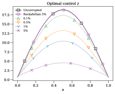
(a) (b)

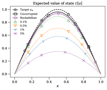
Figure 1: Example 1: (a) Optimal controls for the true, uncorrupted problem, the corrupted problem at varying corruption levels (dotted lines), and the Rockafellian relaxation at 5% corruption. (b) The expected value of the corresponding solutions to the state equation (27) in each case. Corruption levels are defined by (30).

Fig. 1(a) shows $z^{\ast}_{\rm true}$ and $z^{\ast}_{\rm corrupted}$ for varying corruption levels

(30) $$\text{\% corruption}:=100\cdot\epsilon,$$

while Fig. 1(b) shows the expected value of the corresponding solutions to the state equation (27). In contrast to the simple example in Section 2.1, the optimal control for the corrupted problem appears to converge to that of the uncorrupted one as $\epsilon\downarrow 0$ (as seen in Fig. 1); however, the convergence is slow, as there are nontrivial errors even at 0.1% corruption.

Consider now the bivariate Rockafellian $\Phi_{\epsilon}:L^{2}(\Omega)\times\mathbb{R}^{2}\to\overline{\mathbb{R}}$,

(31) $$\Phi_{\epsilon}(z,t):=\frac{1}{2}\sum_{i=1}^{2}(p_{\epsilon,i} +t_{i})\|s(\xi_{\epsilon,i},\,z)-u_{\star}\|_{L^{2}(0,1)}^{2}+\frac{\alpha}{2}\|z\|_{L^{2}(0,1)}^{2}$$

$$+\frac{\theta}{2}\|t\|^{2}_{2}+\iota_{\Delta}(p_{\epsilon}+t),$$

where $\theta>0$, $\xi_{\epsilon,1}=0.2$, $\xi_{\epsilon,2}=2$, and the indicator function $\iota_{\Delta}$ constrains $p_{\epsilon}+t$ to be a probability vector in $\mathbb{R}^{2}$ (see (13)), which is equivalent to the constraint that $t_{1}+t_{2}=0$ and $-p_{\epsilon,i}\leq t_{i}\leq 1-p_{\epsilon,i}$, $i\in\{1,2\}$.

In practice we enforce the equality constraint by eliminating $t_{1}$ via $t_{1}=-t_{2}$. The Rockafellian $\Phi_{\epsilon}(z,t_{2})$ is then optimized with the projected gradient descent method with backtracking line search based on the Armijo condition; here the projection enforces the bound constraints $-p_{\epsilon,2}\leq t_{2}\leq 1-p_{\epsilon,2}$. The initial guesses are $z(x)=1$ (as before) and $t_{2}=0$.

Fig. 1(a) shows the resulting optimal control $z^{\ast}_{\rm Rock}$ for $\epsilon=0.05$ (5% corruption) and $\theta=1$. By optimizing the relaxed Rockafellian $\Phi_{\epsilon}$, we recover the minimizer $z^{\ast}_{\rm true}$ to the uncorrupted problem, as desired; the absolute error

$$\|z^{\ast}_{\rm true}-z^{\ast}_{\rm Rock}\|_{L^{2}(0,1)}\leq\|z^{\ast}_{\rm true}-z^{\ast}_{\rm Rock}\|_{L^{\infty}(0,1)}=5.55\cdot 10^{-2}.$$

Similar results are obtained for the other corruption levels (0.1%, 0.5%, or 1%).

Example 2: For $d\in\mathbb{N}$ and $\sigma\in\mathbb{R}_{+}$, consider next setting the coefficient

$$a(x,\xi)=e^{\sigma\sum_{k=1}^{d}\sqrt{\lambda_{k}}\sin(x/\sqrt{\lambda_{k}})\xi_{k}},\qquad\lambda_{k}=\frac{4}{(2k-1)^{2}\pi^{2}},$$

where each $\xi_{k}$ are independent and normally distributed with zero mean and unit variance; here the argument in the exponential is a truncated KKL expansion for a rescaled Brownian motion on the interval $\Omega=(0,1)$.

The expectation value in (21) is approximated with a sample average approximation (SAA) using $N$ samples; the objective function then becomes

(32) $$\varphi(z)=\frac{1}{2}\sum_{i=1}^{N}p_{i}\|s(\xi^{(i)},z)-u_{\star}\|_{L^{2}(0,1)}^{2}+\frac{\alpha}{2}\|z\|_{L^{2}(0,1)}^{2},$$

where $p_{i}=1/N$ for all $i$ and the samples $\xi^{(i)}\sim\mathcal{N}(0,I_{d})$ are all independent (here $I_{d}$ is the $d\times d$ identity matrix). Define the target function as $u_{\star}(x)=1$.

In all cases, we take $d=50$ terms in the truncated KKL expansion and $N=1000$ SAA samples. In the uncorrupted case, we take $\sigma=0.4$, while in the corrupted cases, we select the first $M\in\mathbb{N}$ samples ($M<N$) and increase their variance through the map $\xi\mapsto 10\,\xi$, which amounts to setting $\sigma=4$ for those samples. Optimization is done with the SciPy [39] implementation of the BFGS algorithm; the algorithm terminates whenever the norm of gradient of the objective function is less than $10^{-5}$, which is the default setting. In all cases, the initial guess $z(x)=1$.

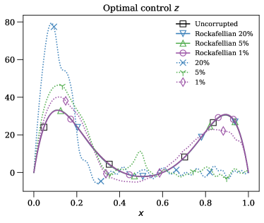
(a) (b)

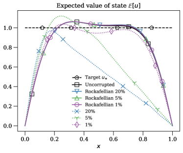
Figure 2: Example 2: (a) Optimal controls for the true, uncorrupted problem, as well as for the corrupted problem (dotted lines) and the corresponding Rockafellian relaxations at varying corruption levels. (b) The expected value of the corresponding solutions to the state equation (27) in each case. Corruption levels are defined by (33).

With the corruption level defined as

(33) $$\text{\% corruption}:=100\cdot M/N,$$

Fig. 2(a) shows that even at just 1% corruption, there are severe differences between $z^{\ast}_{\rm corrupted}$ and $z^{\ast}_{\rm true}$, i.e. the minimizers of (32) with and without corruption, respectively. These differences grow with increasing corruption levels. Fig. 2(b) shows the corresponding expected values of the corrupted state variables are also quite different from the uncorrupted one.

To recover $z_{\rm true}^{\ast}$ in the presence of corrupted data samples, define the bivariate Rockafellian $\Phi:L^{2}(0,1)\times\mathbb{R}^{N}\to\overline{\mathbb{R}}$:

(34) $$\Phi(z,t):=\frac{1}{2}\sum_{i=1}^{N}(p_{i}+t_{i})\|s(\xi^{(i)},z)-u_{\star}\|_{L^{2}(0,1)}^{2}+\frac{\alpha}{2}\|z\|_{L^{2}(0,1)}^{2}+\theta\|t\|_{1}+\iota_{\Delta}(p+t).$$

As the role of the perturbation variable here is to identify (and remove) outlier sample points, $t$ is measured in the $l_{1}$ norm for its well known sparsity-promoting property; this choice is inspired by the statistical learning experiments described in [36, Section 6], where corrupted labels in the contexts of computer vision and text analytics were properly removed.

The experiments in [36] also inspired the optimization method for (34); an alternating-direction heuristic is adopted in which we first fix $t=0$ and compute $z^{\ast}\in\operatorname*{argmin}\Phi(z,0)$ using the BFGS method. The result is then used to compute the solution to the linear program $t^{\ast}\in\operatorname*{argmin}\Phi(z^{\ast},t)$ using SciPy’s implementation of the simplex method. This process is repeated until the absolute $l_{1}$ distance between successive $t^{\ast}$ values is smaller than some $\tau$; in particular we take $\tau=10^{-5}$, consistent with the BFGS stopping criteria quoted in Example 1 above.

The linear program solve in the alternating-direction approach naturally allows the $p+t\in\Delta$ constraint to be satisfied exactly; in particular this constraint imposes the pointwise bounds $-p_{i}\leq t_{i}\leq 1-p_{i}$ for each $1\leq i\leq N$. In practice, to prevent the linear program solver from “greedily” identifying a handful of samples $\xi^{(i)}$ at which

$$\|s(\xi^{(i)},z)-u_{\star}\|_{L^{2}(0,1)}^{2}$$

is the smallest and subsequently deleting all of the other samples (even those that are “clean”, i.e. uncorrupted), we additionally impose the more stringent pointwise bounds $-p_{i}\leq t_{i}\leq p_{i}$ for each $i$.

Fig. 2(a) shows the optimal controls $z^{\ast}_{\rm Rock}$ for (34) with $\theta=5\cdot 10^{-2}$ at 1%, 2%, and 10% corruption levels; the true optimal control $z^{\ast}_{\rm true}$ in each case is indeed recovered, as desired. Fig. 2(b) shows that the corresponding expected values of the Rockafellian state variables are much more accurate than the corrupted counterparts. Table 1 shows the relative $L^{2}$ errors in the optimal controls, as well as the ratio of errors for the corrupted and Rockafellian cases, as defined by

(35) $$\qquad E_{\rm rel}(z):=\frac{\|z-z_{\rm true}^{\ast}\|_{L^{2}(0,1)}}{\|z_{\rm true}^{\ast}\|_{L^{2}(0,1)}},\qquad\mathcal{E}_{\rm ratio}:=\frac{E_{\rm rel}(z^{\ast}_{\rm corrupted})}{E_{\rm rel}(z^{\ast}_{\rm Rock})}.$$

The errors for $z_{\rm Rock}^{\ast}$ are all one to two orders of magnitude smaller than the corresponding ones in the corrupted cases, i.e. $\mathcal{E}_{\rm ratio}$ is large. Although not shown in Fig. 2, the table also shows that Rockafellian relaxation can even recover the optimal controls at a 40% corruption level. In all cases, the Rockafellian perturbation variable $t$ identifies and removes at least 70% of the corrupted data points, while less than 3% of the clean, uncorrupted points are incorrectly removed. In general these percentages will change as a function of $\theta$, which we discuss below in Section 4.3.

Corruption level	$E_{\rm rel}(z^{\ast}_{\rm Rock})$	$\mathcal{E}_{\rm ratio}$	Corrupted deleted	Clean deleted
1%	$6.84\cdot 10^{-3}$	37.4	7/10=70%	26/990=2.62%
5%	$7.72\cdot 10^{-3}$	97.8	40/50=80%	23/950=2.42%
20%	$8.96\cdot 10^{-3}$	115.4	171/200=85.5%	16/800=2.00%
40%	$2.20\cdot 10^{-2}$	47.3	336/400=84%	11/600=1.83%

Table 1: Example 2 with $\theta=5\cdot 10^{-2}$: relative $L^{2}$ errors $E_{\rm rel}$ between the Rockafellian and true optimal controls, as well as the ratio of $L^{2}$ errors $\mathcal{E}_{\rm ratio}$ for the corrupted and Rockafellian optimal controls; see (35). Also included are the fraction of corrupted and clean sample points correctly and incorrectly removed by the perturbation variable $t$, respectively. Corruption levels defined by (33).

Example 3: For the final example, we consider corruptions to the support $\Xi$ to a probability distribution $\mathbb{P}$, as in Section 3.3. Take

(36) $$a(x,\xi)=\frac{1}{\xi+3\sin(10\pi x)},$$

and in the uncorrupted case, let $\xi=3.5$ almost surely; for the corrupted case, let $\xi$ be uniformly distributed on the interval $[3.5-\delta,3.5+\delta]$, where $\delta\in(0,0.5)$. Notice that that contrast ratio

(37) $$\sup_{x\in[0,1]}a(x,\xi)/\inf_{x\in[0,1]}a(x,\xi)$$

of the oscillations is large when $\xi$ takes on values close to $3$.

Since the Dirac measure is not suitable for the theory developed in Section 3.3, for conceptual purposes one could instead take the uncorrupted random variable $\xi$ to be uniformly distributed on the interval $[3.5-\nu,3.5+\nu]\subset\Xi:=\mathbb{R}$, where $0<\nu\ll 1$. The corruption map $\eta:\Xi\to\Xi$ would then be $\eta(\xi)=(\delta/\nu)\xi+3.5(1-\delta/\nu),$ which of course tends to the identity as $\delta\searrow\nu$.

The expectation value in (21) is discretized with standard Gaussian quadrature with $N=8$ points, and optimization in both the uncorrupted and corrupted cases is done with SciPy’s BFGS method with the default settings, as in Example 2. The target function $u_{\star}$ is the piecewise constant function

$$u_{\star}(x)=\begin{cases}1,\qquad&x\in[0,0.5)\\ 5,\qquad&x\in[0.5,1],\end{cases}$$

the initial guess $z(x)=x-x^{2}$, and $\alpha=10^{-6}$.

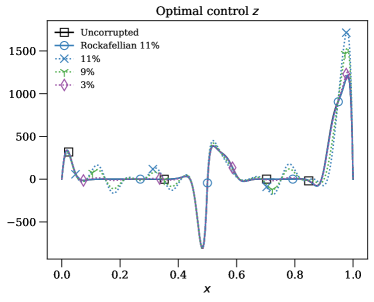
(a) (b)

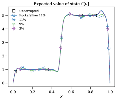
Figure 3: Example 3: (a) Optimal controls for the true, uncorrupted problem, as well as for the corrupted problems (dashed lines) and the corresponding Rockafellian relaxations at varying corruption levels. (b) The expected value of the corresponding solutions to the state equation (27) in each case. Corruption levels are defined by (38).

With the corruption level defined as

(38) $$\text{\% corruption}:=100\cdot\left(\frac{3.5-\delta}{3.5}\right),$$

Fig. 3(a) shows that while a $\sim$3% corruption (corresponding to $\delta=0.1$) has little effect on the optimal control (on the scale of the plot), this is no longer true for $\sim$9% and $\sim$11% corruptions (corresponding to $\delta=0.3$ and $\delta=0.4$, respectively). The principal differences between the corrupted optimal controls $z^{\ast}_{\rm corrupted}$ and true, uncorrupted one $z^{\ast}_{\rm true}$ are (i) the incorrect value of the functions’ peak near the right endpoint of the domain (at $x\approx 0.98$) and (ii) the presence of large-amplitude oscillations in the regions $0.05\lesssim x\lesssim 0.4$ and $0.6\lesssim x\lesssim 0.85$. These oscillations can also be observed in the plots of the expected value of the state variables, shown in Fig. 3(b).

To recover $z_{\rm true}^{\ast}$ in the presence of increased uncertainty in $\xi$, we optimize the following bivariate Rockafellian $\Phi:L^{2}(0,1)\times L^{2}(\Xi;\Xi)\to\mathbb{R}$:

(39) $$\Phi(z,t):=\frac{1}{2}\int_{\Xi_{\delta}}\|s(\tilde{\xi} +t(\tilde{\xi}),z)-u_{\star}\|_{L^{2}(0,1)}^{2}\rho(\tilde{\xi})\,d\tilde{\xi}+\frac{\alpha}{2}\|z\|^{2}_{L^{2}(0,1)}$$

$$+\frac{\theta}{2}\int_{\Xi_{\delta}}|t(\tilde{\xi})|^{2}\rho(\tilde{\xi})\,d\tilde{\xi},$$

where $\theta>0$, $\Xi_{\delta}=[3.5-\delta,3.5+\delta]$, $\rho(\tilde{\xi})=\mathds{1}_{\Xi_{\delta}}(\tilde{\xi})/(2\delta)$, and $\mathds{1}_{S}$ denotes the characteristic function on the set $S$; here we use $\tilde{\xi}$ to denote the corrupted random variable. We additionally enforce the bound constraints on the Rockafellian variable $t(\tilde{\xi})$:

$$3.5-\delta\leq\tilde{\xi}+t(\tilde{\xi})\leq 3.5+\delta,$$

so that the superposition $\tilde{\xi}+t(\tilde{\xi})$ does not take values outside of the support of $\rho(\tilde{\xi})$.

As in Example 2, the Rockafellian (39) is optimized with an alternating direction heuristic. With the initial guess of $t(\tilde{\xi})=0$, we first compute $z^{\ast}\in\operatorname*{argmin}\Phi(z,0)$ using the BFGS method and subsequently compute $t^{\ast}\operatorname*{argmin}\Phi(z^{\ast},t)$ using projected gradient descent with backtracking line search based on the Armijo criteria. This process is repeated until the absolute distance in $L^{2}(\Xi;\Xi)$ between successive $t^{\ast}$ values is smaller than $\tau=10^{-5}$. Note that the Fréchet derivative of the objective $\Phi$ with respect to $t$ is given by

(40) $$\frac{\delta\Phi}{\delta t}(\tilde{\xi})=\theta\,t(\tilde{\xi})-\int_{0}^{1}\frac{\partial}{\partial t}a\big{(}x,\tilde{\xi}+t(\tilde{\xi})\big{)}\nabla u(x,\tilde{\xi})\cdot\nabla p(x,\tilde{\xi})\,d\tilde{\xi},$$

where $p(x,\tilde{\xi})$ is the solution to the adjoint equation

$$-\frac{d}{dx}\Big{(}a\big{(}x,\tilde{\xi}+t(\tilde{\xi})\big{)}\frac{d}{dx}p(x,\tilde{\xi})\Big{)} =u(x,\tilde{\xi})-u_{\star}(x),\qquad(x,\tilde{\xi})\in(0,1)\times\Xi_{\delta}$$

$$p(0,\tilde{\xi})=p(1,\tilde{\xi}) =0.$$

This calculation assumes, of course, differentiability of the coefficient $a(x,\tilde{\xi})$ with respect to $\tilde{\xi}$, which is true for (36) on the domain $\Xi_{\delta}$.

Corruption level	$E_{\rm rel}(z^{\ast}_{\rm Rock})$	$\mathcal{E}_{\rm ratio}$	$\mathcal{V}_{\rm ratio}$
3%	$6.25\cdot 10^{-3}$	5.70	$1.361\cdot 10^{3}$
9%	$1.20\cdot 10^{-2}$	22.2	$9.626\cdot 10^{2}$
11%	$1.94\cdot 10^{-2}$	21.6	$7.612\cdot 10^{2}$

Table 2: Example 3 with $\theta=10^{-1}$: relative $L^{2}$ errors $E_{\rm rel}$ between the Rockafellian and true optimal controls, as well as the ratio of $L^{2}$ errors $\mathcal{E}_{\rm ratio}$ for the corrupted and Rockafellian optimal controls; see (35). Also included is the ratio of variances in the $L^{2}$ norm of the state variables for the corrupted and Rockafellian controls, as defined by (41). Corruption levels defined by (38).

Fig. 3(a) shows that the optimal control $z^{\ast}_{\rm Rock}$ for (39) at $\theta=10^{-1}$ properly matches $z^{\ast}_{\rm true}$ even at $\sim$11% corruption, and Fig. 3(b) shows the expected value of corresponding state variables match as well; the same results hold at lower corruption levels (not shown). Table 2 lists the relative $L^{2}$ errors (defined by (35)) in the Rockafellian optimal controls, which are a factor of more than five (respectively, twenty) times smaller than the relative errors for the corrupted controls at $\sim$3% (resp., $\sim$9% and $\sim$11%) corruption.

Owing to larger contrast ratios of $a(x,\tilde{\xi})$ at lower values of $\tilde{\xi}$ (see (37)), the variance in the $L^{2}$ norm of the corrupted state variables increases with increasing $\delta$. In contrast, the corresponding variance for the Rockafellian state variable is considerably smaller. This is quantified in Table 2, which shows the variance ratio

(41) $$\mathcal{V}_{\rm ratio}:=\frac{\text{Var}(u_{\rm corrupted})}{\text{Var}(u_{\rm Rock})}$$

where $\text{Var}(u):=\mathbb{E}[(\|u(\cdot,\xi)\|_{L^{2}}-\mathbb{E}[\|u(\cdot,\xi)\|_{L^{2}}])^{2}]$. This reduction in the variance is explained by the extremely low spread in the values of $\tilde{\xi}+t^{\ast}_{\rm Rock}(\tilde{\xi})$. Indeed, the expected values of this random variable range between approximately $3.511$ and $3.545$ for the three corruption levels tested, while the largest standard deviation is smaller than $7\cdot 10^{-3}$; essentially, the objective function (39) in this case is minimized whenever the Rockafellian variable $t(\tilde{\xi})$ alters the stochastic optimal control problem to be an (approximately) deterministic one.

4.3 Impact of $\theta$ parameter

As remarked in the preceding subsection, minimizers $z^{\ast}$ and $t^{\ast}$ of Rockafellian objective functionals will depend on the value of the regularization parameter $\theta_{\epsilon}$. Theorem 3.1 stipulates that a Rockafellian will Gamma converge to the corresponding, uncorrupted one when both $\theta_{\epsilon}\to\infty$ and $\theta_{\epsilon}\|\rho_{\epsilon}-\rho\|_{T}^{q}\to 0$ (where $T$ is an $L^{q}$ norm) as $\epsilon\downarrow 0$; in other words, $\theta_{\epsilon}$ should grow as the size of the corruption vanishes, but not too quickly. Analogous conditions are needed in Theorem 3.3 and Theorem 3.4.

These conditions are consistent with intuition; $\theta$ values that are too large will prevent the perturbation variable $t$ from meaningfully altering any corrupted problem data. If $\theta$ is sufficiently small, however, there is the possibility that $t$ “greedily” alters the problem data too much in an effort to reduce the objective functional. In the context of corrupted empirical samples, for example (as considered in Section 3.2), this corresponds to improperly removing “clean”, uncorrupted samples.

$\theta$	$E_{\rm rel}(z^{\ast}_{\rm Rock})$	$\mathcal{E}_{\rm ratio}$	Corrupted deleted	Clean deleted
$5\cdot 10^{-3}$	$4.92\cdot 10^{-2}$	5.62	19/20=95%	416/980=42.4%
$5\cdot 10^{-2}$	$7.23\cdot 10^{-3}$	38.3	14/20=70%	25/980=2.55%
$5\cdot 10^{-1}$	$1.43\cdot 10^{-2}$	19.4	3/20=15%	0/980=0.00%

Table 3: Results from Example02 at various $\theta$ values and 2% corruption (as defined by (33)). $E_{\rm rel}$ and $\mathcal{E}_{\rm ratio}$ are defined by (35).

This intuition is backed up by numerical experiments at varying $\theta$ values. As an illustration, consider again Example 2 in Section 4.2 at 2% corruption. Table 3 shows that while the relative $L^{2}$ error is $\mathcal{O}\left(10^{-2}\right)$ or smaller for $\theta$ at three different orders of magnitude, the error is smallest when most (70%) of the corrupted samples are deleted and few (less than 3%) of the clean sampled are removed.

For Rockafellian relaxations on the support of a probability distribution (as considered in Section 3.3), the value of $\theta$ affects the variance reduction property observed in Example 3 of Section 4.2. Recall that the variance in $\tilde{\xi}+t_{\rm Rock}^{\ast}(\tilde{\xi})$ (denoting the superposition of the corrupted random variable and the optimal perturbation variable $t$) was quite small at $\theta=10^{-1}$; for $\theta=10^{-2}$, the variance is even smaller, while for $\theta=1$ it is larger. At smaller $\theta$ values, then, variance in the state variable $u_{\rm Rock}(x,\xi)$ is lower; the opposite is true at larger $\theta$ values. This is quantified by the ratio $\mathcal{V}_{\rm ratio}$ (defined in (41)) in Table 4 for the case of $\sim$11% corruption. For all values of $\theta$, the relative $L^{2}$ error between the Rockafellian optimal control and the true, uncorrupted one is $\mathcal{O}\left(10^{-2}\right)$.

$\theta$	$E_{\rm rel}(z^{\ast}_{\rm Rock})$	$\mathcal{E}_{\rm ratio}$	$\mathcal{V}_{\rm ratio}$
$10^{-2}$	$1.95\cdot 10^{-2}$	21.4	$7.054\cdot 10^{4}$
$10^{-1}$	$1.94\cdot 10^{-2}$	21.6	$7.612\cdot 10^{2}$
$1$	$5.99\cdot 10^{-2}$	6.99	$1.223\cdot 10^{1}$

Table 4: Results from Example03 at various $\theta$ values and 11% corruption (as defined by (38)). $E_{\rm rel}$ and $\mathcal{E}_{\rm ratio}$ are defined by (35), and $\mathcal{V}_{\rm ratio}$ is defined by (41).

4.4 Computational cost

In general, the computational cost of optimizing a bivariate Rockafellian is larger than optimizing its (potentially corrupted) single-variable counterpart; the enhanced resiliency to data corruption afforded by Rockafellian relaxation does not come for free.

For example, the total number of gradient descent iterations in Example 1 taken to minimize the Rockafellian (31) was 3187, compared to only 446 iterations for the corrupted problem. Note, however, that computing the gradient of (31) with respect to $t$ is essentially free, since the relatively expensive terms $\|s(\xi_{\epsilon,i},z)-u_{\star}\|^{2}_{L^{2}(0,1)}$ which appear in this gradient are already needed for an objective function evaluation. Hence, the additional computational cost comes essentially from the need for additional evaluations of the objective functional (31) and its gradient with respect to the control $z$. This is true for the alternating direction (ADI) heuristics employed in Examples 2 and 3 as well.

Indeed, the heuristic for Example 2 entails alternating between a BFGS solve for the control $z$ and a linear program solve for the perturbation variable $t$ with $\mathcal{O}\left(1000\right)$ unknowns. The cost of the latter will of course increase with the number of discrete samples, but for large-scale PDECO problems this will likely remain (significantly) smaller than the cost of the former.

The ADI heuristic for Example 3 involves a standard projected gradient descent (with line search) for $t$, and in practice we observe this to converge quite rapidly—always in fewer than ten iterations. Note that constructing the gradient with respect to $t$ only requires calculating an integral over the spatial domain $\Omega$ for each stochastic collocation point used in the discretization of the probability sample space; see (40).

$\theta$	$N_{\rm iters}$, 2%	$N_{\rm iters}$, 20%	$N_{\rm evals}$, 2%	$N_{\rm evals}$, 20%
$5\cdot 10^{-3}$	537	1640	2024	6251
$5\cdot 10^{-2}$	514	1852	1953	7065
$5\cdot 10^{-1}$	351	2697	1333	10303

Table 5: Example 2: total number of BFGS iterations, denoted $N_{\rm iter}$, as well as the total number of evalations of the objective functional (34) and its gradient with respect to the control $z$, denoted $N_{\rm evals}$, at various $\theta$ values and two corruption levels (as defined by (33)).

Since the additional cost for Rockafellian relaxation comes primarily from the additional work to optimize over the control variable $z$, we quantify how much is needed for representative cases of Examples 2 and 3 in Table 5 and Table 6, respectively.

For Example 2, optimizing the corrupted objective functional (32) at 2% corruption without Rockafellian relaxation using the BFGS method took 189 total iterations, which includes 719 evaluations of both the objective functional and its gradient with respect to the control $z$. Table 5 shows that optimizing the Rockafellian (34) at this level of corruption was about two to three times more expensive, depending on $\theta$. At 20% corruption, 412 BFGS iterations and 1576 objective functional and gradient evaluations were required to optimize (32), while the cost to optimize the Rockafellian ranged between approximately four to six and a half times more expensive.

For Example 3, the total number of BFGS iterations (as well as objective functional and gradient evaluations) needed to optimize the Rockafellian (39) in $z$ was slightly less than twice the amount needed to optimize the corrupted objective functional (21). This was true both for 9% and 11% corruption levels, and there was little to no variation as a function of $\theta$; see Table 6 for the precise numbers for the Rockafellian case.

$\theta$	$N_{\rm iters}$, 9%	$N_{\rm iters}$, 11%	$N_{\rm evals}$, 9%	$N_{\rm evals}$, 11%
$10^{-2}$	1140	1142	4961	4989
$10^{-1}$	1140	1150	4961	4982
$1$	1138	1147	4953	4967

Table 6: Example 3: total number of BFGS iterations, denoted $N_{\rm iter}$, as well as the total number of evalations of the objective functional (39) and its gradient with respect to the control $z$, denoted $N_{\rm evals}$, at various $\theta$ values and two corruption levels (as defined by (38)).

5 Conclusions

We introduce a framework based on Rockafellian relaxation for general stochastic PDE constrained optimization problems that is robust to perturbations in the the precise form of the problem uncertainty. Theoretical $\Gamma$-convergence results are shown, and numerical examples of elliptic, stochastic optimal control problems illustrate the framework’s utility for outlier detection and removal and for variance reduction.

There are numerous potential avenues for future research. Firstly, the framework can be employed in a much broader range of contexts than considered here. Two possible examples are data assimilation problems and full waveform inversion problems, because of the potential for corrupted empirical measurements exists in those contexts.

It may also be reasonable to consider different forms of the bivariate, Rockafellian functional. The work here considered $L^{p}$ norms for the perturbation variable $t$, but other choices, for example the Kullback-Leibler divergence or the Wasserstein distance, are possible and may have their own advantages.

Finally, there is room to develop theory for how to best optimize Rockafellian objectives. Based on the numerical experiments described in Section 4.2, an inexact trust region framework seems promising for optimally balancing computational cost and efficiency [11, 15, 2].

Appendix A Proof of Theorem 3.3

Proof A.1.

The proof for the cases $q=\infty$ and $q\in[1,\infty)$ proceed identically; here we assume the latter. Let $T$ denote $l^{q}(\mathbb{R}^{N})$.

We first establish the limit superior condition in Definition 2.1. Suppose that $(z,t)\in Z\times T$; since $\Phi(z,t)=\infty$ for $t\neq 0$ (in which case the condition holds trivially), suppose $t=0$. Constructing the strongly converging sequences as $z_{\epsilon}=z$ and $t_{\epsilon}=p-p_{\epsilon}$ for all $\epsilon>0$, we have

$$\Phi_{\epsilon}(z_{\epsilon},t_{\epsilon})=f_{0}(z)+\sum_{i=1}^{N}p_{i}g\big{(}s(\xi_{i},z)\big{)}+\frac{\theta_{\epsilon}}{q}\|p-p_{\epsilon}\|_{q}^{q}+\underbrace{\iota_{\Delta}(p)}_{=0},$$

which implies

$$\limsup_{\epsilon\downarrow 0}\Phi_{\epsilon}(z_{\epsilon},t_{\epsilon})=f_{0}(z)+\sum_{i=1}^{N}p_{i}g\big{(}s(\xi_{i},z)\big{)}+\underbrace{\limsup_{\epsilon\downarrow 0}\frac{\theta_{\epsilon}}{q}\|p-p_{\epsilon}\|_{q}^{q}}_{=0}=\Phi(z,0)$$

by assumption, as desired.

Next, we consider an arbitrary sequence $(z_{\epsilon},t_{\epsilon})_{\epsilon}$ converging weakly to some $(z,t)$ in the product topology on $Z\times T$. Since $T$ is a finite-dimensional normed space, note that weak and strong convergence are equivalent. Since $f_{0}$ is proper lsc and the indicator $\iota_{\Delta}$ is also lsc (as $\Delta$ is a closed, convex set in $\mathbb{R}^{N}$), we have

$$\liminf_{\epsilon\downarrow 0}\Phi_{\epsilon}(z_{\epsilon},t_{\epsilon})\geq f_{0}(z)+\liminf_{\epsilon\downarrow 0}\sum_{i=1}^{N}(p_{\epsilon,i}+t_{\epsilon,i}) g\big{(}s(\xi_{i},z_{\epsilon})\big{)}$$

$$+\liminf_{\epsilon\downarrow 0}\frac{\theta_{\epsilon}}{q}\|t_{\epsilon}\|_{q}^{q} +\iota_{\Delta}(p+t).$$

Since $g$ too is sequentially weakly lsc and bounded below, and since and $p_{\epsilon}+t_{\epsilon}\to p+t$,

$$\liminf_{\epsilon\downarrow 0}\sum_{i=1}^{N}(p_{\epsilon,i}+t_{\epsilon,i})g\big{(}s(\xi_{i},z_{\epsilon})\big{)}\geq\sum_{i=1}^{N}(p_{i}+t_{i})g\big{(}s(\xi_{i},z)\big{)}$$

which then gives

$$\liminf_{\epsilon\downarrow 0}\Phi_{\epsilon}(z_{\epsilon},t_{\epsilon})\geq f_{0}(z)+\sum_{i=1}^{N}(p_{i}+t_{i})g\big{(}s(\xi_{i},z)\big{)}+\liminf_{\epsilon\downarrow 0}\frac{\theta_{\epsilon}}{q}\|t_{\epsilon}\|_{q}^{q}+\iota_{\Delta}(p+t).$$

If $t=0$, then the right-hand side of this inequality is trivially greater than or equal to $\Phi(z,0)$. If $t\neq 0$, then the Rockafellian $\Phi(z,t)=\infty$, while the sequence $\|t_{\epsilon}\|_{q}$ is necessarily bounded below by some positive constant for $\epsilon$ sufficiently small. Since $\theta_{\epsilon}\to\infty$, this gives $\liminf_{\epsilon\downarrow 0}\Phi_{\epsilon}(z_{\epsilon},t_{\epsilon})=\Phi(z,t)=\infty,$ as desired.

Appendix B Proof of Theorem 3.4

Proof B.1.

We assume that $q\in[1,\infty)$, as the case of $q=\infty$ is nearly the same.

Establishing first the limit superior condition, suppose that $(z,t)\in Z\times T$. Since the condition trivially holds for $t(\xi)\neq 0$ a.s., suppose otherwise. Constructing the sequences as $z_{\epsilon}=z$ and $t_{\epsilon}=\eta_{\epsilon}-I$ for all $\epsilon>0$, we have

$$\Phi_{\epsilon}(z_{\epsilon},t_{\epsilon})=f_{0}(z)+\mathbb{E}\left[g\big{(}s(\xi,z)\big{)}\right]+\frac{\theta_{\epsilon}}{q}\|\eta_{\epsilon}-I\|_{T}^{q}.$$

Taking the limit superior of both sides gives $\limsup_{\epsilon\downarrow 0}\Phi_{\epsilon}(z_{\epsilon},t_{\epsilon})=\Phi(z,0),$ as desired.

Next, consider an arbitrary sequence $(z_{\epsilon},t_{\epsilon})_{\epsilon\in\mathbb{R}_{+}}$ that converges strongly to some $(z,t)\in Z\times T$ in the product topology, and first suppose that $t(\xi)=0$ a.s. As detailed in the proof of Theorem 3.1, it suffices to establish the limit inferior condition along a subsequence for which

(42) $$\eta_{\epsilon^{\prime}}(\xi)+t_{\epsilon^{\prime}}(\xi)\to\xi\qquad\text{a.s. in }\Xi.$$

For ease of exposition, we abuse notation by reverting the subsequence index back to $\epsilon$ and proceed to work with the subsequence.

The weak convergence $z_{\epsilon}\rightharpoonup z$ and (42) imply by Section 3.3 that $s(\eta_{\epsilon}(\xi)+t_{\epsilon}(\xi),z_{\epsilon})\rightharpoonup s(\xi,z)$ in $U$, while the lsc property of $g$ implies $\liminf_{\epsilon\downarrow 0}g\big{(}s(\eta_{\epsilon}(\xi)+t_{\epsilon}(\xi),z_{\epsilon})\big{)}\geq g\big{(}s(\xi,z)\big{)}.$ Since $g$ is coercive and $f_{0}$ is lsc, the result $\liminf_{\epsilon\downarrow 0}\Phi_{\epsilon}(z_{\epsilon},t_{\epsilon})\geq\Phi(z,0)$ follows from Fatou’s lemma.

Finally, consider an arbitrary sequence $(z_{\epsilon},t_{\epsilon})_{\epsilon\in\mathbb{R}_{+}}$ that converges to some $(z,t)$, with $t(\xi)\neq 0$ a.s. Because $\Phi(z,t)=\infty$, $g$ and $f_{0}$ are bounded below and proper, respectively, the result $\liminf_{\epsilon\downarrow 0}\Phi_{\epsilon}(z_{\epsilon},t_{\epsilon})=\Phi(z,t)$ follows from the fact that

$$\liminf_{\epsilon\downarrow 0}\frac{\theta_{\epsilon}}{q}\|t_{\epsilon}\|_{T}^{q}=\infty,$$

as $\|t_{\epsilon}\|_{T}$ is necessarily bounded below and $\theta_{\epsilon}\to\infty$.

Appendix C Proofs of propositions from Section 4.1

Proof C.1 (Proof of Proposition 4.2).

Let $\xi\in\Xi$ such that (22) holds, the Lax-Milgram theorem and weak convergence of $z_{\epsilon}$ imply the uniform bound

$$\|s_{\epsilon}(\xi,z_{\epsilon})\|_{H^{1}_{0}(\Omega)}\leq\frac{C_{p}}{a_{\ast}}\|z_{\epsilon}\|_{L^{2}(\Omega)}\leq\frac{C_{p}}{a_{\ast}}\sup_{\epsilon}\|z_{\epsilon}\|_{L^{2}(\Omega)}<\infty$$

(where $C_{p}$ is the Poincaré constant in $\Omega$). The Banach-Alaoglu theorem then guarantees there exists some $u(\cdot,\xi)\in H^{1}_{0}(\Omega)$ such that

(43) $$s(\xi,z_{\epsilon})\rightharpoonup u(\cdot,\xi)\text{ in }H^{1}_{0}(\Omega)$$

up to a subsequence (here we abuse notation and keep the original index $\epsilon$). We now show that $u(\cdot,\xi)=s(\xi,z)$, i.e., it solves the variational problem (23).

Let $v\in H^{1}_{0}(\Omega)$ be arbitrary. Due to uniform boundedness of $a$ in (22) and weak convergence of $s(\xi,z_{\epsilon})$ from (43), we obtain that

$$\lim_{\epsilon\downarrow 0}\int_{\Omega}a(x,\xi)\nabla s(\xi,z_{\epsilon})(x)\cdot\nabla v(x)\,dx=\int_{\Omega}a(x,\xi)\nabla u(x,\xi)\cdot\nabla v(x)\,dx.$$

Since $\left\langle z_{\epsilon},v\right\rangle_{L^{2}(\Omega)}\to\left\langle z,v\right\rangle_{L^{2}(\Omega)}$ by supposition, Definition 4.1 implies

$$\left\langle z,v\right\rangle_{L^{2}(\Omega)}=\lim_{\epsilon\downarrow 0}\int_{\Omega}a(x,\xi)\nabla s(\xi,z_{\epsilon})(x)\cdot\nabla v(x)\,dx=\int_{\Omega}a(x,\xi)\nabla u(x,\xi)\cdot\nabla v(x)\,dx,$$

so that indeed, $u(\cdot,\xi)=s(\xi,z)$, as desired. Weak convergence of the full sequence follows by uniqueness of limits of sequences of real numbers.

Proof C.2 (Proof of Proposition 4.3).

The proof proceeds similarly to that of Proposition 4.2. The Lax-Milgram theorem and weak convergence of $z_{\epsilon}$ imply the uniform bound

(44) $$\|s(\xi_{\epsilon},z_{\epsilon})\|_{H^{1}_{0}(\Omega)}\leq\frac{C_{p}}{a_{\ast}}\|z_{\epsilon}\|_{L^{2}(\Omega)}\leq\frac{C_{p}}{a_{\ast}}\sup_{\epsilon}\|z_{\epsilon}\|_{L^{2}(\Omega)}<\infty$$

(where, again, $C_{p}$ is the Poincaré constant in $\Omega$). The Banach-Alaoglu theorem guarantees there exists some $u\in H^{1}_{0}(\Omega)$ such that

(45) $$s(\xi_{\epsilon},z_{\epsilon})\rightharpoonup u\text{ in }H^{1}_{0}(\Omega)$$

up to a subsequence (here we abuse notation and keep the original index $\epsilon$). We now show that $u=s(\xi,z)$, i.e., it solves the variational problem (23).

Let $v\in H^{1}_{0}(\Omega)$ be arbitrary. Due to uniform boundedness of $a$ in (22) and the weak convergence (45), we have

(46) $$\lim_{\epsilon\downarrow 0}\int_{\Omega}a(x,\xi)\nabla s(\xi_{\epsilon},z_{\epsilon})(x)\cdot\nabla v(x)\,dx=\int_{\Omega}a(x,\xi)\nabla u(x)\cdot\nabla v(x)\,dx.$$

By supposition, $\left\langle z_{\epsilon},v\right\rangle_{L^{2}(\Omega)}\to\left\langle z,v\right\rangle_{L^{2}(\Omega)}$, so that by Definition 4.1 and (46),

(47) $$\left\langle z,v\right\rangle_{L^{2}(\Omega)}=\lim_{\epsilon\downarrow 0} \int_{\Omega}\big{[}a(x,\xi_{\epsilon})-a(x,\xi)\big{]}\nabla s(\xi_{\epsilon},z_{\epsilon})(x)\cdot\nabla v(x)\,dx$$

$$+\int_{\Omega}a(x,\xi)\nabla u(x)\cdot\nabla v(x)\,dx.$$

The desired result follows if the first term on the right-hand side of (47) equals zero. By the Cauchy-Schwartz inequality,

$$\Big{|}\int_{\Omega}\big{[}a(x,\xi_{\epsilon})-a(x,\xi)\big{]} \nabla s(\xi_{\epsilon},z_{\epsilon})(x)\cdot\nabla v(x)\,dx\Big{|}$$

$$\leq\operatorname*{ess\,sup}_{x\in\Omega}|a(x,\xi)-a(x,\xi_{\epsilon})|\,\,\|u_{\epsilon}(\cdot,\xi_{\epsilon})\|_{H^{1}_{0}(\Omega)}\|v\|_{H^{1}_{0}(\Omega)},$$

so that both sides vanish as $\epsilon\downarrow 0$ by the uniform bound (44) and the presumed continuity of $a$.

Weak convergence of the full sequence follows by uniqueness of limits of sequences of real numbers.

References

- [1] R. Agarwal, D. Schuurmans, and M. Norouzi, An optimistic perspective on offline reinforcement learning, in International Conference on Machine Learning, PMLR, 2020, pp. 104–114.
- [2] H. Antil, D. P. Kouri, M.-D. Lacasse, and D. Ridzal, eds., Frontiers in PDE-constrained optimization, vol. 163 of The IMA Volumes in Mathematics and its Applications, Springer, New York, 2018.
- [3] A. Aravkin and D. Davis, Trimmed statistical estimation via variance reduction, Mathematics of Operations Research, 45 (2020), pp. 292–322.
- [4] T. Arbogast and J. Bona, Method of Applied Mathematics, Department of Mathematics, University of Texas at Austin, 2008.
- [5] A. Ben-Tal and A. Nemirovski, Robust solutions of linear programming problems contaminated with uncertain data, Mathematical programming, 88 (2000), pp. 411–424.
- [6] J. Blanchet, J. Li, S. Lin, and X. Zhang, Distributionally robust optimization and robust statistics, arXiv preprint arXiv:2401.14655, (2024).
- [7] J. Blanchet, J. Li, M. Pelger, and G. Zanotti, Automatic outlier rectification via optimal transport, arXiv preprint arXiv:2403.14067, (2024).
- [8] J. F. Bonnans and A. Shapiro, Perturbation analysis of optimization problems, Springer Science & Business Media, 2013.
- [9] J. Cao and R. Gao, Contextual decision-making under parametric uncertainty and data-driven optimistic optimization, Optimization Online, 2021.
- [10] P. Chen and J. O. Royset, Performance bounds for pde-constrained optimization under uncertainty, SIAM Journal on Optimization, 33 (2023), pp. 1828–1854.
- [11] A. R. Conn, N. I. M. Gould, and P. L. Toint, Trust-region methods, MPS/SIAM Series on Optimization, Society for Industrial and Applied Mathematics (SIAM), Philadelphia, PA; Mathematical Programming Society (MPS), Philadelphia, PA, 2000.
- [12] E. A. Feinberg, P. O. Kasyanov, and J. O. Royset, Epi-convergence of expectation functions under varying measures and integrands, Journal of Convex Analysis, 30 (2023), pp. 917–936.
- [13] J.-y. Gotoh, M. J. Kim, and A. E. Lim, A data-driven approach to beating SAA out of sample, Oper. Res., (2023), pp. 1–13. Articles in advance.
- [14] C. R. Harris et al., Array programming with NumPy, Nature, 585 (2020), pp. 357–362.
- [15] M. Heinkenschloss and L. Vicente, Analysis of inexact trust-region SQP algorithms, SIAM J. Optim., 12 (2002), pp. 283–302.
- [16] N. Jiang and W. Xie, Distributionally favorable optimization: A framework for data-driven decision-making with endogenous outliers, SIAM Journal on Optimization, 34 (2024), pp. 419–458.
- [17] K. Karhunen, Zur spektraltheorie stochastischer prozesse, Ann. Acad. Sci. Fennicae, AI, 34 (1946).
- [18] P. Kolvenbach, O. Lass, and S. Ulbrich, An approach for robust pde-constrained optimization with application to shape optimization of electrical engines and of dynamic elastic structures under uncertainty, Optimization and Engineering, 19 (2018), pp. 697–731.
- [19] D. D. Kosambi, Statistics in function space, Journal of the Indian Mathematical Society, 7 (1943), pp. 76–88.
- [20] D. P. Kouri, A measure approximation for distributionally robust pde-constrained optimization problems, SIAM Journal on Numerical Analysis, 55 (2017), pp. 3147–3172.
- [21] D. P. Kouri and T. M. Surowiec, Risk-averse pde-constrained optimization using the conditional value-at-risk, SIAM Journal on Optimization, 26 (2016), pp. 365–396.
- [22] D. P. Kouri and T. M. Surowiec, Epi-regularization of risk measures, Mathematics of Operations Research, 45 (2020), pp. 774–795.
- [23] O. Lass and S. Ulbrich, Model order reduction techniques with a posteriori error control for nonlinear robust optimization governed by partial differential equations, SIAM Journal on Scientific Computing, 39 (2017), pp. S112–S139.
- [24] M. Loéve, Fonctions aléatoires du second ordre, Processus Stochastique et Mouvement Brownien, (1948).
- [25] J. Martínez-Frutos and F. P. Esparza, Optimal control of PDEs under uncertainty: An introduction with application to optimal shape design of structures, Springer, 2018.
- [26] J. Milz and M. Ulbrich, An approximation scheme for distributionally robust pde-constrained optimization, SIAM Journal on Control and Optimization, 60 (2022), pp. 1410–1435.
- [27] H. Narasimhan, A. K. Menon, W. Jitkrittum, and S. Kumar, Learning to reject meets ood detection: Are all abstentions created equal?, arXiv preprint arXiv:2301.12386, (2023).
- [28] V. A. Nguyen, S. Shafieezadeh Abadeh, M.-C. Yue, D. Kuhn, and W. Wiesemann, Calculating optimistic likelihoods using (geodesically) convex optimization, Advances in Neural Information Processing Systems, 32 (2019).
- [29] V. A. Nguyen, S. Shafieezadeh Abadeh, M.-C. Yue, D. Kuhn, and W. Wiesemann, Optimistic distributionally robust optimization for nonparametric likelihood approximation, Advances in Neural Information Processing Systems, 32 (2019).
- [30] V. A. Nguyen, N. Si, and J. Blanchet, Robust bayesian classification using an optimistic score ratio, in International Conference on Machine Learning, PMLR, 2020, pp. 7327–7337.
- [31] M. Norton, A. Takeda, and A. Mafusalov, Optimistic robust optimization with applications to machine learning, arXiv preprint arXiv:1711.07511, (2017).
- [32] S. T. Rachev and W. Römisch, Quantitative stability in stochastic programming: The method of probability metrics, Mathematics of Operations Research, 27 (2002), pp. 792–818.
- [33] R. T. Rockafellar, Convex functions and dual extremum problems, PhD thesis, Harvard University, 1963.
- [34] R. T. Rockafellar, Convex Analysis, vol. 28, Princeton University Press, 1970.
- [35] J. O. Royset, Risk-adaptive approaches to stochastic optimization: a survey, SIAM Review, (to appear).
- [36] J. O. Royset, L. L. Chen, and E. Eckstrand, Rockafellian relaxation and stochastic optimization under perturbations, arXiv preprint arXiv:2204.04762v4, (2022).
- [37] J. O. Royset and R. J-B Wets, An Optimization Primer, Springer, 2022.
- [38] J. Song and C. Zhao, Optimistic distributionally robust policy optimization, arXiv preprint arXiv:2006.07815, (2020).
- [39] P. Virtanen et al., SciPy 1.0: Fundamental Algorithms for Scientific Computing in Python, Nature Methods, 17 (2020), pp. 261–272.
- [40] R. L. Wheeden and A. Zygmund, Measure and Integral: An Introduction to Real Analysis, CRC Press, Taylor & Francis Group, 2nd ed., 2015.
- [41] P. Zheng, R. Barber, R. J. Sorensen, C. J. Murray, and A. Y. Aravkin, Trimmed constrained mixed effects models: formulations and algorithms, Journal of Computational and Graphical Statistics, 30 (2021), pp. 544–556.