Divergences in the effective loop interaction of the Chern-Simons bosons with leptons. The unitary gauge case

Abstract

In this paper, we consider the extension of the Standard Model with Chern-Simons type interaction. There is a new vector massive boson (Chern-Simons bosons) in this extension. Using only three-particle dimension-4 interaction of the Chern-Simons bosons with vector bosons of the SM we consider effective loop interaction of a new vector boson with leptons. We consider the renormalizability of this loop interaction and conclude that for the case of computation of loop diagrams in the unitary gauge, we can not get rid of the divergences in the effective interaction of the Chern-Simons bosons with leptons.

1 Introduction

Despite the success of the Standard Model (SM) [1] in describing numerous collider experiments, SM is not a complete theory because it cannot explain phenomena such as active neutrino oscillation (see e.g. [2, 3, 4]), baryon asymmetry of the Universe (see e.g. [5, 6, 7]), dark matter (see e.g. [8, 9, 10]). In all likelihood, the SM needs to be extended to include new particles and new interactions.

It may turn out that SM has a hidden sector with many new particles and some of these particles are not relevant to solving problems of the SM. We do not detect new particles because they are quite heavy or light but very feebly interact with particles of the SM. If the new particles are quite heavy and can not be produced at current accelerators, we hope they will be detected at more powerful future accelerators such as FCC [11, 12]. But if the new particles are light they can be found at existing accelerators nowadays, see e.g. [13, 14, 15], in the intensity frontier experiments such as MATHUSLA [16], FACET [17], FASER [18, 19], SHiP [20, 21], NA62 [22, 23, 24], DUNE [25, 26], etc.

We don’t know what type of particles of the new physics they will be. They can be scalar [27, 28, 29], pseudoscalar (axionlike) [30, 31, 32, 33], fermion [34, 35, 36, 37], or vector (dark photons) [38, 39, 40] particles, see reviews [16, 21]. In this paper, we consider the extension of the Standard Model with Chern-Simons type interaction with a new massive vector boson (Chern-Simons bosons or CS bosons in the following). The Chern-Simons interactions appear in various theoretical models, including extra dimensions and the string theory, see e.g. [41, 42, 43, 44, 45, 46]. The minimal gauge-invariant Lagrangian of the interaction of the CS bosons with SM particles has a form of 6-dimension operators [21, 47]:

$$\mathcal{L}_{1} =\frac{C_{Y}}{\Lambda_{Y}^{2}}\cdot X_{\mu}(\mathfrak{D}_{\nu}H)^{\dagger}HB_{\lambda\rho}\cdot\epsilon^{\mu\nu\lambda\rho}+h.c.,$$ (1.1)

$$\mathcal{L}_{2} =\frac{C_{SU(2)}}{\Lambda_{SU(2)}^{2}}\cdot X_{\mu}(\mathfrak{D}_{\nu}H)^{\dagger}F_{\lambda\rho}H\cdot\epsilon^{\mu\nu\lambda\rho}+h.c.,$$ (1.2)

where $\Lambda_{Y}$, $\Lambda_{SU(2)}$ are new scales of the theory; $C_{Y}$, $C_{SU(2)}$ are new dimensionless coupling constants; $\epsilon^{\mu\nu\lambda\rho}$ is the Levi-Civita symbol ($\epsilon^{0123}=+1$); $X_{\mu}$ – CS vector bosons; $H$ – scalar field of the Higgs doublet; $B_{\mu\nu}=\partial_{\mu}B_{\nu}-\partial_{\nu}B_{\mu}$, $F_{\mu\nu}={\displaystyle-ig\sum_{i=1}^{3}\frac{\tau^{i}}{2}V^{i}_{\mu\nu}}$ – field strength tensors of the $U_{Y}(1)$ and $SU_{W}(2)$ gauge fields of the SM.

After the electroweak symmetry breaking Lagrangians (1.1), (1.2) generate (among other terms of higher dimensions) Lagrangian of three fields interactions in the form of 4-dimension operators:

$$\mathcal{L}_{CS}=c_{z}\epsilon^{\mu\nu\lambda\rho}X_{\mu}Z_{\nu}\partial_{\lambda}Z_{\rho}+c_{\gamma}\epsilon^{\mu\nu\lambda\rho}X_{\mu}Z_{\nu}\partial_{\lambda}A_{\rho}+\left\{c_{w}\epsilon^{\mu\nu\lambda\rho}X_{\mu}W_{\nu}^{-}\partial_{\lambda}W_{\rho}^{+}+h.c.\right\},$$ (1.3)

where $A_{\mu}$ is the electromagnetic field; $W^{\pm}_{\mu}$ and $Z_{\mu}$ are fields of the weak interaction; and $c_{z}$, $c_{\gamma}$, $c_{w}$ are some dimensionless independent coefficients. Coefficients $c_{z}$ and $c_{\gamma}$ are real, but $c_{w}$ can be complex. As one can see, there is no direct interaction of the CS vector boson $X_{\mu}$ with fields of the matter.

If one rewrites the coefficients before operators in (1.1), (1.2) as $C_{Y}/\Lambda_{Y}^{2}=C_{1}/v^{2}$ and $C_{SU(2)}/\Lambda_{SU(2)}^{2}=C_{2}/v^{2}$, where $C_{1}=c_{1}+{\rm i}c_{1{\rm i}}$ and $C_{2}=c_{2}+{\rm i}c_{2{\rm i}}$ are dimensionless coefficients, then in unitary gauge one can obtain

$$c_{z}=-c_{1{\rm i}}g^{\prime}+\frac{c_{2}}{2}g^{2},$$ (1.4)

$$c_{\gamma}=c_{1{\rm i}}g+\frac{c_{2}}{2}gg^{{}^{\prime}},$$ (1.5)

$$c_{w}=\frac{c_{2}+{\rm i}c_{2{\rm i}}}{2}g^{2}\equiv\Theta_{W1}+{\rm i}\Theta_{W2}.$$ (1.6)

Effective interaction of the CS bosons with quarks of different flavours was considered in [48, 49, 50]. It was shown that in this case divergent part of the loop diagrams (containing only $W^{\pm}$ bosons) is proportional to a non-diagonal element of the unity matrix $U^{+}U$ ($U$ is the Cabibbo–Kobayashi–Maskawa matrix) and is removed. It allows one to construct an effective Lagrangian of the interaction of the CS bosons with quarks of different flavours and compute the GeV-scale CS bosons’ production in decays of meson. At the same time, it was shown that effective interaction of the CS bosons with quarks of the same flavours or with leptons contains divergence. This divergence can not be removed via counterterms of the CS boson interaction with fermions because the initial Lagrangian does not contain these terms.

The question of the effective interaction of the CS bosons with fermions of the same flavour is very important. Solving this problem will make it possible to find all decay channels of the CS boson and compute the CS boson’s lifetime, which in turn will allow us to compute the sensitivity region of the intensity frontier experiments for searching the CS boson.

In this paper, we will consider the effective interaction of the CS bosons with leptons and compute all corresponding loop diagrams (containing $W^{\pm}$, $Z$ bosons, and photons) in the unitary gauge. We will be interested in the processes of decay of the CS boson into a lepton pair $\ell^{+}\ell^{-}$ ($\ell=e,\mu,\tau$) and neutrinos. We want to check whether there will be a cancellation of divergences when taking into account all corresponding diagrams.

2 Lepton pair production in the CS boson decays.
Direct computations

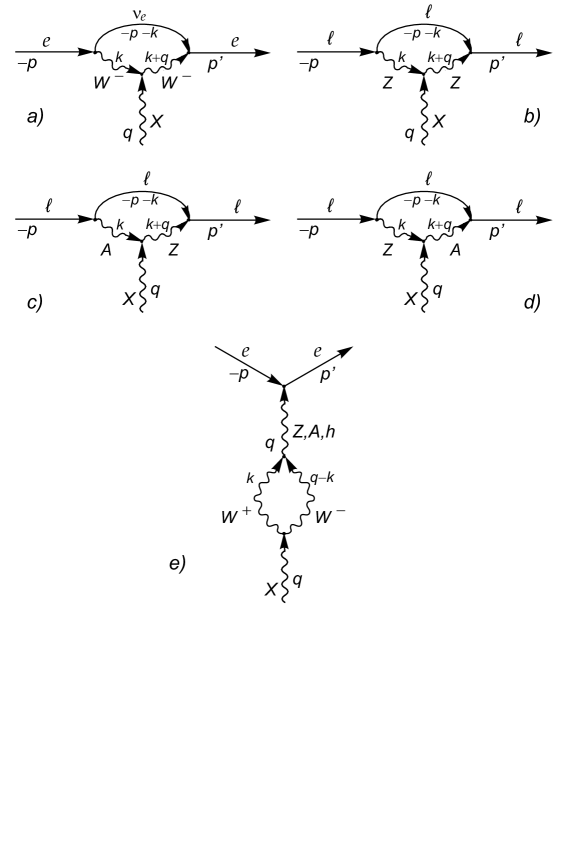
Figure 1: Diagrams of the CS boson’s decay into leptons in the unitary gauge.

In the unitary gauge to compute the amplitude of the CS boson’s decay into leptons one has to take into account the following diagrams presented in Fig.1, where for the vertex of the CS boson interaction with vector fields (1.3) we have the following rules, see Fig.2

$$XWW\qquad-(c_{W}p-c_{W}^{*}k)_{\lambda}\epsilon^{\mu\nu\lambda\rho},$$ (2.1)

$$XZZ\qquad-c_{Z}p_{\lambda}\epsilon^{\mu\nu\lambda\rho},$$ (2.2)

$$XZA\qquad-c_{\gamma}p_{\lambda}\epsilon^{\mu\nu\lambda\rho}.$$ (2.3)

One also has to take into account two diagrams with vertex $XZZ$ in Fig.1b (line with a derivative from $Z$ from the left side or the right side of the diagram).

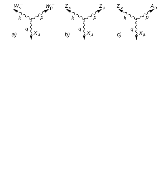
Figure 2: Vertex diagrams of the interaction of the CS boson with vector fields of the SM in accordance with (1.3).

2.1 Production via $XWW$ interaction

Lepton pair production via $XWW$ interaction is described by the diagrams a and e in Fig.1. The amplitude of the lepton pair production via diagram e in Fig.1 is identically equal to zero due to the presence of the Levi-Civita symbol in the vertex of $XWW$ interaction. The amplitude of the lepton pair production in the CS boson decays via diagram a in Fig.1 is given by

$$M^{WW}_{fi}=\frac{g^{2}}{2}\bar{\ell}(p^{\prime})\hat{P}_{R}I^{\bar{\mu}}_{W}\hat{P}_{L}\ell(-p)\epsilon^{\lambda_{X}}_{\bar{\mu}},$$ (2.4)

where $g$ is $SU(2)_{L}$ coupling, $P_{L(R)}=(1-(+)\gamma^{5})/2$,

$$I^{\bar{\mu}}_{W}=\int\frac{d^{4}k}{(2\pi)^{4}}\gamma^{\mu}G_{\nu}(-p-k)D^{W}_{\mu{\bar{\rho}}}(k+q)\left[c_{\omega}(k+q)_{\bar{\lambda}}+c^{\ast}_{\omega}k_{\bar{\lambda}}\right]D^{W}_{\bar{\nu}\nu}(k)\gamma^{\nu}\epsilon^{{\bar{\mu}}{\bar{\nu}}{\bar{\lambda}}{\bar{\rho}}}$$ (2.5)

and

$$G_{f}(p)=\frac{m_{f}+\not p}{m_{f}^{2}-p^{2}},\quad D_{\mu\nu}^{V}(k)=g_{\mu\nu}-\frac{k_{\mu}k_{\nu}}{M_{V}^{2}}$$ (2.6)

are propagators for vector field $V$ in unitary gauge and for fermion $f$.

After computation using the technique of $\alpha$ (Schwinger) representation, see e.g. [51], one can get similarly to [50]:

$$I^{\bar{\mu}}_{W}=\hat{\Lambda}_{0}^{\nu\ell W}\left\{\vphantom{\frac{1}{2}}\gamma_{\bar{\rho}}(\not{\!\mathcal{P}}-\not{\!p})\gamma_{\bar{\nu}}\left\{\Theta_{W}^{1}(q-2\mathcal{P})_{\bar{\lambda}}+i\Theta^{2}_{W}q_{\bar{\lambda}}\right\}+\right.\\ +\left.\frac{q_{\bar{\lambda}}}{M_{W}^{2}}\mathcal{P}_{\bar{\nu}}\gamma_{\bar{\rho}}\left[c_{w}^{*}\left\{2(p\mathcal{P})+\not{\!q\,}\not{\!\mathcal{P}}-\not{\!q\,}\not{\!p}\right\}-2\Theta_{W}^{1}\mathcal{P}^{2}+2i\Theta_{W}^{2}\not{\!p}\not{\!\mathcal{P}}\right]\right\}\epsilon^{{\bar{\mu}}{\bar{\nu}}{\bar{\lambda}}{\bar{\rho}}}+\\ +\hat{\Lambda}_{1}^{\nu\ell W}\left\{(-i\Theta_{W}^{1})\gamma_{\bar{\rho}}\gamma_{\bar{\lambda}}\gamma_{\bar{\nu}}+\frac{q_{\bar{\lambda}}}{M_{W}^{2}}\left[i\frac{c_{w}^{*}}{2}\gamma_{\bar{\rho}}{\not{\!q\,}}\gamma_{\bar{\nu}}-6i\Theta_{W}^{1}\gamma_{\bar{\rho}}\mathcal{P}_{\bar{\nu}}-\Theta_{W}^{2}\gamma_{\bar{\rho}}\not{\!p}\gamma_{\bar{\nu}}\right]\right\}\epsilon^{{\bar{\mu}}{\bar{\nu}}{\bar{\lambda}}{\bar{\rho}}}.$$ (2.7)

where

$$\mathcal{P}=xp+yq$$ (2.8)

and $\hat{\Lambda}_{0}^{fgV}$, $\hat{\Lambda}_{1}^{fgV}$ are integral operators acting on some function:

$$\hat{\Lambda}_{0}^{fgV}u(x,y)=\frac{i\pi^{2}}{(2\pi)^{4}}\int_{0}^{1}\!\!dx\int_{0}^{1-x}\!\!\!dy\frac{u(x,y)}{D^{fgV}(x,y)},$$ (2.9)

$$\hat{\Lambda}_{1}^{fgV}u(x,y)=\frac{-\pi^{2}}{(2\pi)^{4}}\int_{0}^{1}\!\!dx\int_{0}^{1-x}\!\!\!dy\,u(x,y)\ln\frac{\Lambda^{2}x}{D^{fgV}(x,y)},$$ (2.10)

$$D^{fgV}(x,y)=xm_{f}^{2}-x(1-x)m_{g}^{2}+(1-x)M_{V}^{2}-y(1-x-y)M_{X}^{2},$$ (2.11)

$\Lambda$ is some constant with dimension of mass (it should be put to infinity in the final result, $\Lambda\rightarrow\infty$). So, the divergent part of the loop diagram is hidden in the operator $\hat{\Lambda}_{1}^{fgV}$.

2.2 Production via $XZZ$ interaction

The amplitude of the lepton pair production via $XZZ$ interaction is described by the diagram b in Fig.1

$$M^{ZZ}_{fi}=\frac{g^{2}}{4\cos^{2}\theta_{W}}\,\bar{\ell}(p^{\prime})\,\,\hat{\overline{P}}_{Z}I_{Z}^{\bar{\mu}}\hat{P}_{Z}\,\ell(-p)\epsilon^{\lambda_{X}}_{\bar{\mu}},$$ (2.12)

where

$$\hat{P}_{Z}=t_{3}^{\ell}(1-\gamma^{5})-2q_{\ell}\sin^{2}\theta_{W},\qquad\hat{\overline{P}}_{Z}=t_{3}^{\ell}(1+\gamma^{5})-2q_{\ell}\sin^{2}\theta_{W}$$ (2.13)

and

$$I_{Z}^{\bar{\mu}}=\int\frac{d^{4}k}{(2\pi)^{4}}\gamma^{\mu}G_{\ell}(-p-k)D^{Z}_{\mu{\bar{\rho}}}(k+q)c_{Z}(2k+q)_{\bar{\lambda}}D^{Z}_{\bar{\nu}\nu}(k)\gamma^{\nu}\epsilon^{{\bar{\mu}}{\bar{\nu}}{\bar{\lambda}}{\bar{\rho}}},$$ (2.14)

where $G_{f}(p)$ and $D_{\mu\nu}^{V}$ were defined in (2.6), $\theta_{W}$ is Weinberg angle, $q_{f}$ is electric charge of lepton $\ell$ in the unites of proton charge and $t_{3}^{\ell}$ is the third component of the weak isospin ($+1/2$ for neutrinos and $-1/2$ for electrically charged leptons).

One can get

$$I^{\bar{\mu}}_{Z}=m_{\ell}c_{Z}\hat{\Lambda}_{0}^{\ell\ell Z}\left\{\gamma_{\bar{\rho}}\gamma_{\bar{\nu}}(q\,-2\mathcal{P})_{\bar{\lambda}}+\frac{q\,_{\bar{\lambda}}}{M_{Z}^{2}}\mathcal{P}_{\bar{\nu}}\not{\!q\,}\gamma_{\bar{\rho}}\right\}\epsilon^{{\bar{\mu}}{\bar{\nu}}{\bar{\lambda}}{\bar{\rho}}}+\\ +c_{Z}\hat{\Lambda}_{0}^{\ell\ell Z}\left\{\vphantom{\frac{1}{2}}\gamma_{\bar{\rho}}(\not{\!\mathcal{P}}-\not{\!p})\gamma_{\bar{\nu}}(q-2\mathcal{P})_{\bar{\lambda}}+\frac{q_{\bar{\lambda}}}{M_{Z}^{2}}\mathcal{P}_{\bar{\nu}}\gamma_{\bar{\rho}}\left(-2\mathcal{P}^{2}+2(p\mathcal{P})+\not{\!q\,}\not{\!\mathcal{P}}-\not{\!q\,}\not{\!p}\right)\right\}\epsilon^{{\bar{\mu}}{\bar{\nu}}{\bar{\lambda}}{\bar{\rho}}}+\\ +ic_{Z}\hat{\Lambda}_{1}^{\ell\ell Z}\left\{-\gamma_{\bar{\rho}}\gamma_{\bar{\lambda}}\gamma_{\bar{\nu}}+\frac{q_{\bar{\lambda}}}{M_{Z}^{2}}\left[\frac{\gamma_{\bar{\rho}}{\not{\!q}}\gamma_{\bar{\nu}}}{2}-6\gamma_{\bar{\rho}}\mathcal{P}_{\bar{\nu}}\right]\right\}\epsilon^{{\bar{\mu}}{\bar{\nu}}{\bar{\lambda}}{\bar{\rho}}},$$ (2.15)

where $\hat{\Lambda}_{0}^{\ell\ell Z}$, $\hat{\Lambda}_{1}^{\ell\ell Z}$ are defined in (2.9) and (2.10).

2.3 Production via $XZA$ interaction

The amplitude of the lepton pair production via $XZA$ interaction is described by the diagrams c,d in Fig.1

$$M_{fi}^{AZ}=\frac{gq_{f}e}{2\cos\theta_{W}}\,\bar{\ell}(p^{\prime})I_{ZA}^{\bar{\mu}}\ell(-p)\epsilon^{\lambda_{X}}_{\bar{\mu}},$$ (2.16)

where

$$I_{ZA}^{\bar{\mu}}=c_{\gamma}\int\frac{d^{4}k}{(2\pi)^{4}}\left[\hat{\overline{P}}_{Z}\gamma^{\mu}G_{\ell}(-p-k)D^{Z}_{\mu{\bar{\rho}}}(k+q)k_{\bar{\lambda}}D^{\gamma}_{\bar{\nu}\nu}(k)\gamma^{\nu}+\right.\\ +\left.\gamma^{\mu}G_{\ell}(-p-k)D^{\gamma}_{\mu{\bar{\rho}}}(k+q)(k+q)_{\bar{\lambda}}D^{Z}_{\bar{\nu}\nu}(k)\gamma^{\nu}\hat{P}_{Z}\right]\epsilon^{{\bar{\mu}}{\bar{\nu}}{\bar{\lambda}}{\bar{\rho}}}=c_{\gamma}\hat{\overline{P}}_{Z}I_{ZA1}^{\bar{\mu}}+c_{\gamma}I_{ZA2}^{\bar{\mu}}\hat{P}_{Z},$$ (2.17)

$\hat{P}_{Z}$, $\hat{\overline{P}}_{Z}$ are defined by (2.13), $G_{f}(p)$ and $D_{\mu\nu}^{V}$ were defined in (2.6).

One can get

$$I_{ZA1}^{\bar{\mu}}=-m_{f}\left[\hat{\Lambda}_{0}^{1,\ell Z\gamma}\left\{\gamma_{\bar{\rho}}+\frac{q_{\bar{\rho}}}{M_{Z}^{2}}\,(\not{\!\mathcal{P}}-\not{\!q\,})\right\}\gamma_{\bar{\nu}}\mathcal{P}_{\bar{\lambda}}+\Lambda_{1}^{(1\gamma)}\frac{i}{2}\frac{q_{\bar{\rho}}}{M_{Z}^{2}}\,\gamma_{\bar{\lambda}}\gamma_{\bar{\nu}}\right]\epsilon^{{\bar{\mu}}{\bar{\nu}}{\bar{\lambda}}{\bar{\rho}}}+\\ +\hat{\Lambda}_{0}^{1,\ell Z\gamma}\left\{\gamma_{\bar{\rho}}(\not{\!p}-\not{\mathcal{\!P}})\gamma_{\bar{\nu}}+\frac{q_{\bar{\rho}}}{M_{Z}^{2}}\left[(\not{\mathcal{\!P}}\not{\!p}-\mathcal{P}^{2})\gamma_{\bar{\nu}}-\not{\!q}\,(\not{\!p}-\not{\mathcal{\!P}})\gamma_{\bar{\nu}}\right]\right\}\mathcal{P}_{\bar{\lambda}}\epsilon^{{\bar{\mu}}{\bar{\nu}}{\bar{\lambda}}{\bar{\rho}}}+\\ +\Lambda_{1}^{1,\ell Z\gamma}\frac{i}{2}\left\{-\gamma_{\bar{\rho}}\gamma_{\bar{\lambda}}+\frac{q_{\bar{\rho}}}{M_{Z}^{2}}\left(\gamma_{\bar{\lambda}}\not{\!p}+\not{\!q}\,\gamma_{\bar{\lambda}}-6\mathcal{P}_{\bar{\lambda}}\right)\right\}\gamma_{\bar{\nu}}\epsilon^{{\bar{\mu}}{\bar{\nu}}{\bar{\lambda}}{\bar{\rho}}}$$ (2.18)

and

$$I_{ZA2}^{\bar{\mu}}=-m_{f}\left[\hat{\Lambda}_{0}^{2,\ell Z\gamma}\gamma_{\bar{\rho}}\left\{\gamma_{\bar{\nu}}(\mathcal{P}_{\bar{\lambda}}-q_{\bar{\lambda}})+\frac{q_{\bar{\lambda}}}{M_{Z}^{2}}\not{\!\mathcal{P}}\mathcal{P}_{\bar{\nu}}\right\}+\Lambda_{1}^{(2\gamma)}\frac{i}{2}\gamma_{\bar{\rho}}\frac{q_{\bar{\lambda}}}{M_{Z}^{2}}\gamma_{\bar{\nu}}\right]\epsilon^{{\bar{\mu}}{\bar{\nu}}{\bar{\lambda}}{\bar{\rho}}}+\\ +\hat{\Lambda}_{0}^{2,\ell Z\gamma}\gamma_{\bar{\rho}}\left\{(\not{\!p}-\not{\!\mathcal{P}})(\mathcal{P}_{\bar{\lambda}}-q_{\bar{\lambda}})\gamma_{\bar{\nu}}+\frac{q_{\bar{\lambda}}}{M_{Z}^{2}}(\not{\!p}\not{\!\mathcal{P}}-\mathcal{P}^{2})\mathcal{P}_{\bar{\nu}}\right\}\epsilon^{{\bar{\mu}}{\bar{\nu}}{\bar{\lambda}}{\bar{\rho}}}+\\ +\Lambda_{1}^{2,\ell Z\gamma}\frac{i}{2}\gamma_{\bar{\rho}}\left\{-\gamma_{\bar{\lambda}}\gamma_{\bar{\nu}}+\frac{q_{\bar{\lambda}}}{M_{Z}^{2}}(\not{\!p}\gamma_{\bar{\nu}}-6\mathcal{P}_{\bar{\nu}})\right\}\epsilon^{{\bar{\mu}}{\bar{\nu}}{\bar{\lambda}}{\bar{\rho}}},$$ (2.19)

where $\hat{\Lambda}_{0}^{i,\ell Z\gamma}$, $\hat{\Lambda}_{1}^{i,\ell Z\gamma}$ ($i=1,2$) are integral operators acting on a some function

$$\hat{\Lambda}_{0}^{i,\ell Z\gamma}u(x,y)=i\frac{\pi^{2}}{(2\pi)^{4}}\int_{0}^{1}dx\int_{0}^{1-x}\!\!\!\!dy\frac{u(x,y)}{D^{i,\ell Z\gamma}(x,y)},$$ (2.20)

$$\hat{\Lambda}_{1}^{i,\ell Z\gamma}u(x,y)=-\frac{\pi^{2}}{(2\pi)^{4}}\int_{0}^{1}dx\int_{0}^{1-x}dy\,u(x,y)\ln\frac{\Lambda^{2}x}{D^{i,\ell Z\gamma}(x,y)},$$ (2.21)

and

$$D^{1,\ell Z\gamma}(x,y)=x^{2}m_{\ell}^{2}+yM_{Z}^{2}-y(1-x-y)M_{X}^{2},$$ (2.22)

$$D^{2,\ell Z\gamma}(x,y)=x^{2}m_{\ell}^{2}+(1-x-y)M_{Z}^{2}-y(1-x-y)M_{X}^{2}.$$ (2.23)

3 Combining divergent parts of diagrams in the
direct approach

Let us look only at divergent parts of the diagrams (2.4), (2.12), (2.16) to find the possible conditions for cancellation of divergences. It is the parts containing corresponding operators $\hat{\Lambda}_{1}^{j}$, see (2.10), (2.21). We can see, that different $\hat{\Lambda}_{1}^{j}$ operators contain equal divergent parts

$$\hat{\Lambda}_{1}^{j}=\frac{-\pi^{2}}{(2\pi)^{4}}\int_{0}^{1}\!\!dx\int_{0}^{1-x}\!\!\!dy\,\left[\ln\frac{\Lambda^{2}}{M_{W}^{2}}+\ln\frac{M_{W}^{2}x}{D^{j}(x,y)}\right]=\frac{-\pi^{2}}{2(2\pi)^{4}}\ln\frac{\Lambda^{2}}{M_{W}^{2}}+\hat{\Lambda}_{1}^{j,finite}\\ =L+\hat{\Lambda}_{1}^{j,finite}.$$ (3.1)

We can write the following useful relation for the operator

$$\hat{\Lambda}_{1}^{j}x=L/3+\hat{\Lambda}_{1}^{j,finite}x,$$ (3.2)

where

$$L=\frac{-\pi^{2}}{2(2\pi)^{4}}\ln\frac{\Lambda^{2}}{M_{W}^{2}}\rightarrow\infty.$$ (3.3)

The part of $M_{fi}=M_{fi}^{WW}+M_{fi}^{ZZ}+M_{fi}^{AZ}$ proportional to divergent quantity $L$ is given by

$$M_{fi}^{div}=L\cdot\bar{\ell}(p^{\prime})I^{{\mu}}\ell(-p)\epsilon^{\lambda_{X}}_{\mu},$$ (3.4)

where

$$I^{{\mu}}=A\gamma_{\bar{\rho}}\gamma_{\bar{\lambda}}\gamma_{\bar{\nu}}\epsilon^{{\bar{\mu}}{\bar{\nu}}{\bar{\lambda}}{\bar{\rho}}}+Bq_{\bar{\lambda}}\gamma_{\bar{\rho}}\not{q}\gamma_{\bar{\nu}}\epsilon^{{\bar{\mu}}{\bar{\nu}}{\bar{\lambda}}{\bar{\rho}}}+Cq_{\bar{\lambda}}\gamma_{\bar{\rho}}\not{p}\gamma_{\bar{\nu}}\epsilon^{{\bar{\mu}}{\bar{\nu}}{\bar{\lambda}}{\bar{\rho}}}+Dq_{\bar{\lambda}}\gamma_{\bar{\rho}}p_{\bar{\nu}}\epsilon^{{\bar{\mu}}{\bar{\nu}}{\bar{\lambda}}{\bar{\rho}}},$$ (3.5)

$$A=\gamma^{5}\frac{g}{2}\left[\frac{\Theta_{W}^{1}g}{2}+\frac{c_{z}g}{\cos^{2}\theta_{W}}t_{3}^{f}\left[t_{3}^{f}-2q_{f}\sin^{2}\theta_{W}\right]+\frac{c_{\gamma}q_{f}e}{\cos\theta_{W}}t_{3}^{f}\right]-\\ -\frac{g}{2}\left[\frac{\Theta_{W}^{1}g}{2}+\frac{c_{z}g}{\cos^{2}\theta_{W}}\left(t_{3}^{f}\left[t_{3}^{f}-2q_{f}\sin^{2}\theta_{W}\right]+2q_{f}^{2}\sin^{4}\theta_{W}\right)+\frac{c_{\gamma}q_{f}e}{\cos\theta_{W}}\left(t_{3}^{f}-2q_{f}\sin^{2}\theta_{W}\right)\right],$$ (3.6)

$$B=-\gamma^{5}\frac{g}{4M_{W}^{2}}\left[\frac{c_{w}^{*}g}{2}+c_{z}gt_{3}^{f}\left[t_{3}^{f}-2q_{f}\sin^{2}\theta_{W}\right]+c_{\gamma}q_{f}e\cos\theta_{W}t_{3}^{f}\right]+\\ +\frac{g}{4M_{W}^{2}}\left[\frac{c_{w}^{*}g}{2}+c_{z}g\left(t_{3}^{f}\left[t_{3}^{f}-2q_{f}\sin^{2}\theta_{W}\right]+2q_{f}^{2}\sin^{4}\theta_{W}\right)+c_{\gamma}q_{f}e\cos\theta_{W}\left(t_{3}^{f}-2q_{f}\sin^{2}\theta_{W}\right)\right],$$ (3.7)

$$C=i\Theta_{W}^{2}\frac{g^{2}}{4M_{W}^{2}}(1-\gamma^{5}),$$ (3.8)

$$D=\gamma^{5}\frac{g}{3M_{W}^{2}}\left[\frac{\Theta_{W}^{1}g}{2}+c_{z}gt_{3}^{f}\left[t_{3}^{f}-2q_{f}\sin^{2}\theta_{W}\right]+c_{\gamma}q_{f}e\cos\theta_{W}t_{3}^{f}\right]-\\ -\frac{g}{3M_{W}^{2}}\left[\frac{\Theta_{W}^{1}g}{2}+c_{z}g\left(t_{3}^{f}\left[t_{3}^{f}-2q_{f}\sin^{2}\theta_{W}\right]+2q_{f}^{2}\sin^{4}\theta_{W}\right)+c_{\gamma}q_{f}e\cos\theta_{W}\left(t_{3}^{f}-2q_{f}\sin^{2}\theta_{W}\right)\right].$$ (3.9)

It would be good if there were some relationships between coefficients like (1.4) – (1.6), under which the condition $A=B=C=D=0$ would be satisfied. But that’s not true.

Putting $C=0$, one gets $\Theta_{W}^{2}=0$, so $c_{w}=c_{w}^{*}=\Theta_{W}^{1}$. Unfortunately, there is no relationship between the couplings $\Theta_{W}^{1}$, $c_{Z}$, $c_{\gamma}$ in which the conditions $A=B=D=0$ are simultaneously satisfied.

Expressions (2.5), (2.15), and (2.17) contain linear divergent integrals. They will change when the integration variable is shifted by a constant, as in the case of considering the chiral anomaly, see [52]. However, such a change of variables will cause the value of the integrals to change only by a finite amount. So, expressions for $A$ – $D$ will not change.

4 Conclusions

In this paper, we considerd the extension of the Standard Model with Chern-Simons type interaction. Limiting ourselves to considering only three-particle dimension-4 interaction of the Chern-Simons bosons with vector bosons of the SM (1.3) we considered the effective loop interaction of a new vector boson with leptons.

As was shown in [48, 49, 50] the effective loop interaction (with only $W$-bosons in the loop) of the CS bosons with fermions of different flavours (quarks) does not contain divergences, but interactions with fermions of the same flavours suffer from divergences. But the initial interaction Lagrangian (1.3) has no direct interaction of the CS boson with fermions, so we cannot use counterterms to eliminate the divergences. Therefore, the interaction of the CS bosons with vector bosons of the SM is self-consistent only if divergences will be eliminated accounting for all appropriate loop diagrams including interactions in the loop of types $XWW$, $XZZ$, and $XZA$.

We considered loop diagrams with all possible three-particle vertices, see Fig.1, and concluded that for the case of computation of loop diagrams in the unitary gauge, we can not get rid of the divergences in the effective interaction of the Chern-Simons bosons with fermions of the same flavours (leptons). For definitive conclusions, the problem requires a more detailed consideration within the framework of non-unitary gauge.

References

- [1] W. N. Cottingham and D. A. Greenwood, An Introduction to the Standard Model of Particle Physics. Cambridge University Press, 7, 2023, 10.1017/9781009401685.
- [2] S. M. Bilenky and S. T. Petcov, Massive Neutrinos and Neutrino Oscillations, Rev. Mod. Phys. 59 (1987) 671.
- [3] A. Strumia and F. Vissani, Neutrino masses and mixings and…, hep-ph/0606054.
- [4] P. F. de Salas, D. V. Forero, C. A. Ternes, M. Tortola and J. W. F. Valle, Status of neutrino oscillations 2018: 3 hint for normal mass ordering and improved CP sensitivity, Phys. Lett. B 782 (2018) 633 [1708.01186].
- [5] G. Steigman, Observational tests of antimatter cosmologies, Ann. Rev. Astron. Astrophys. 14 (1976) 339.
- [6] A. Riotto and M. Trodden, Recent progress in baryogenesis, Ann. Rev. Nucl. Part. Sci. 49 (1999) 35 [hep-ph/9901362].
- [7] L. Canetti, M. Drewes and M. Shaposhnikov, Matter and Antimatter in the Universe, New J. Phys. 14 (2012) 095012 [1204.4186].
- [8] P. J. E. Peebles, Dark Matter, Proc. Nat. Acad. Sci. 112 (2015) 2246 [1305.6859].
- [9] V. Lukovic, P. Cabella and N. Vittorio, Dark matter in cosmology, Int. J. Mod. Phys. A 29 (2014) 1443001 [1411.3556].
- [10] G. Bertone and D. Hooper, History of dark matter, Rev. Mod. Phys. 90 (2018) 045002 [1605.04909].
- [11] T. Golling et al., Physics at a 100 TeV pp collider: beyond the Standard Model phenomena, 1606.00947.
- [12] FCC collaboration, A. Abada et al., FCC Physics Opportunities: Future Circular Collider Conceptual Design Report Volume 1, Eur. Phys. J. C 79 (2019) 474.
- [13] V. M. Gorkavenko, Search for Hidden Particles in Intensity Frontier Experiment SHiP, Ukr. J. Phys. 64 (2019) 689 [1911.09206].
- [14] J. Beacham et al., Physics Beyond Colliders at CERN: Beyond the Standard Model Working Group Report, J. Phys. G 47 (2020) 010501 [1901.09966].
- [15] G. Lanfranchi, M. Pospelov and P. Schuster, The Search for Feebly Interacting Particles, Ann. Rev. Nucl. Part. Sci. 71 (2021) 279 [2011.02157].
- [16] D. Curtin et al., Long-Lived Particles at the Energy Frontier: The MATHUSLA Physics Case, Rept. Prog. Phys. 82 (2019) 116201 [1806.07396].
- [17] S. Cerci et al., FACET: A new long-lived particle detector in the very forward region of the CMS experiment, 2201.00019.
- [18] FASER collaboration, A. Ariga et al., Letter of Intent for FASER: ForwArd Search ExpeRiment at the LHC, 1811.10243.
- [19] FASER collaboration, A. Ariga et al., FASER’s physics reach for long-lived particles, Phys. Rev. D 99 (2019) 095011 [1811.12522].
- [20] SHiP collaboration, M. Anelli et al., A facility to Search for Hidden Particles (SHiP) at the CERN SPS, 1504.04956.
- [21] S. Alekhin et al., A facility to Search for Hidden Particles at the CERN SPS: the SHiP physics case, Rept. Prog. Phys. 79 (2016) 124201 [1504.04855].
- [22] SHiP collaboration, P. Mermod, Prospects of the SHiP and NA62 experiments at CERN for hidden sector searches, PoS NuFact2017 (2017) 139 [1712.01768].
- [23] NA62 collaboration, E. Cortina Gil et al., Search for heavy neutral lepton production in decays, Phys. Lett. B 778 (2018) 137 [1712.00297].
- [24] M. Drewes, J. Hajer, J. Klaric and G. Lanfranchi, NA62 sensitivity to heavy neutral leptons in the low scale seesaw model, JHEP 07 (2018) 105 [1801.04207].
- [25] DUNE collaboration, R. Acciarri et al., Long-Baseline Neutrino Facility (LBNF) and Deep Underground Neutrino Experiment (DUNE): Conceptual Design Report, Volume 2: The Physics Program for DUNE at LBNF, 1512.06148.
- [26] DUNE collaboration, B. Abi et al., Prospects for beyond the Standard Model physics searches at the Deep Underground Neutrino Experiment, Eur. Phys. J. C 81 (2021) 322 [2008.12769].
- [27] B. Patt and F. Wilczek, Higgs-field portal into hidden sectors, hep-ph/0605188.
- [28] F. Bezrukov and D. Gorbunov, Light inflaton Hunter’s Guide, JHEP 05 (2010) 010 [0912.0390].
- [29] I. Boiarska, K. Bondarenko, A. Boyarsky, V. Gorkavenko, M. Ovchynnikov and A. Sokolenko, Phenomenology of GeV-scale scalar portal, JHEP 11 (2019) 162 [1904.10447].
- [30] R. D. Peccei and H. R. Quinn, CP Conservation in the Presence of Instantons, Phys. Rev. Lett. 38 (1977) 1440.
- [31] S. Weinberg, A New Light Boson?, Phys. Rev. Lett. 40 (1978) 223.
- [32] F. Wilczek, Problem of Strong and Invariance in the Presence of Instantons, Phys. Rev. Lett. 40 (1978) 279.
- [33] K. Choi, S. H. Im and C. S. Shin, Recent progress in physics of axions or axion-like particles, 2012.05029.
- [34] T. Asaka and M. Shaposhnikov, The MSM, dark matter and baryon asymmetry of the universe, Phys. Lett. B 620 (2005) 17 [hep-ph/0505013].
- [35] T. Asaka, S. Blanchet and M. Shaposhnikov, The nuMSM, dark matter and neutrino masses, Phys. Lett. B 631 (2005) 151 [hep-ph/0503065].
- [36] K. Bondarenko, A. Boyarsky, D. Gorbunov and O. Ruchayskiy, Phenomenology of GeV-scale Heavy Neutral Leptons, JHEP 11 (2018) 032 [1805.08567].
- [37] A. Boyarsky, M. Drewes, T. Lasserre, S. Mertens and O. Ruchayskiy, Sterile neutrino Dark Matter, Prog. Part. Nucl. Phys. 104 (2019) 1 [1807.07938].
- [38] L. B. Okun, LIMITS OF ELECTRODYNAMICS: PARAPHOTONS?, Sov. Phys. JETP 56 (1982) 502.
- [39] B. Holdom, Two U(1)’s and Epsilon Charge Shifts, Phys. Lett. B 166 (1986) 196.
- [40] P. Langacker, The Physics of Heavy Gauge Bosons, Rev. Mod. Phys. 81 (2009) 1199 [0801.1345].
- [41] I. Antoniadis, E. Kiritsis and T. N. Tomaras, A D-brane alternative to unification, Phys. Lett. B 486 (2000) 186 [hep-ph/0004214].
- [42] C. Coriano, N. Irges and E. Kiritsis, On the effective theory of low scale orientifold string vacua, Nucl. Phys. B 746 (2006) 77 [hep-ph/0510332].
- [43] P. Anastasopoulos, M. Bianchi, E. Dudas and E. Kiritsis, Anomalies, anomalous U(1)’s and generalized Chern-Simons terms, JHEP 11 (2006) 057 [hep-th/0605225].
- [44] J. A. Harvey, C. T. Hill and R. J. Hill, Standard Model Gauging of the Wess-Zumino-Witten Term: Anomalies, Global Currents and pseudo-Chern-Simons Interactions, Phys. Rev. D 77 (2008) 085017 [0712.1230].
- [45] P. Anastasopoulos, F. Fucito, A. Lionetto, G. Pradisi, A. Racioppi and Y. S. Stanev, Minimal Anomalous U(1)-prime Extension of the MSSM, Phys. Rev. D 78 (2008) 085014 [0804.1156].
- [46] J. Kumar, A. Rajaraman and J. D. Wells, Probing the Green-Schwarz Mechanism at the Large Hadron Collider, Phys. Rev. D 77 (2008) 066011 [0707.3488].
- [47] I. Antoniadis, A. Boyarsky, S. Espahbodi, O. Ruchayskiy and J. D. Wells, Anomaly driven signatures of new invisible physics at the Large Hadron Collider, Nucl. Phys. B 824 (2010) 296 [0901.0639].
- [48] J. A. Dror, R. Lasenby and M. Pospelov, New constraints on light vectors coupled to anomalous currents, Phys. Rev. Lett. 119 (2017) 141803 [1705.06726].
- [49] J. A. Dror, R. Lasenby and M. Pospelov, Dark forces coupled to nonconserved currents, Phys. Rev. D 96 (2017) 075036 [1707.01503].
- [50] Y. Borysenkova, P. Kashko, M. Tsarenkova, K. Bondarenko and V. Gorkavenko, Production of Chern–Simons bosons in decays of mesons, J. Phys. G 49 (2022) 085003 [2110.14500].
- [51] N. N. Bogolyubov and D. V. Shirkov, QUANTUM FIELDS. Benjamin Cummings, San Francisco, 1983.
- [52] T.-P. Cheng and L.-F. Li, Gauge Theory of Elementary Particle Physics. Oxford University Press, Oxford, UK, 1984.