Abstract

Bipolar Disorder (BD) is a complex disease. It is heterogeneous, both at the phenotypic and genetic level, although the extent and impact of this heterogeneity is not fully understood. One way to assess this heterogeneity is to look for patterns in the subphenotype data, identify a more phenotypically homogeneous set of subjects, and perform a genome-wide association-study (GWAS) and subsequent secondary analyses restricted to this homogeneous subset. Because of the variability in how phenotypic data was collected by the various BD studies over the years, homogenizing the phenotypic data is a challenging task, and so is replication.

As members of the Psychiatric Genomics Consortium (PGC), we have access to the raw genotypes of 18,711 BD cases and 29,738 controls. This amount of data makes it possible for us to set aside the intricacies of phenotype and allow the genetic data itself to determine which subjects define a homogeneous genetic subgroup.

In this paper, we leverage recent advances in heterogeneity analysis to look for distinct homogeneous genetic BD subgroups (or biclusters) that manifest the broad phenotype we think of as Bipolar Disorder.

As our data was generated by $27$ studies and genotyped on a variety of platforms (OMEX, Affymetrix, Illumina), we use a biclustering algorithm capable of covariate-correction. Covariate-correction is critical if we wish to distinguish disease-related signals from those which are a byproduct of ancestry, study or genotyping platform. We rely on the raw genotyped data and do not include any data generated through imputation.

We first apply this covariate-corrected biclustering algorithm to a cohort of $2524$ BD cases and $4106$ controls from the Bipolar Disease Research Network (BDRN: OMEX). We find evidence of genetic heterogeneity delineating a statistically significant bicluster comprising a subset of BD cases which exhibits a disease-specific pattern of differential-expression across a subset of SNPs. This pattern replicates across the remaining data-sets collected by the PGC containing 5781/8289 (OMEX), 3581/7591 (Illumina), and 6825/9752(Affymetrix) cases/controls, respectively.

This bicluster includes subjects diagnosed with bipolar type-I, as well as subjects diagnosed with bipolar type-II. However, the bicluster is enriched for bipolar type-I over type-II and may represent a collection of correlated genetic risk-factors. By investigating the bicluster-informed polygenic-risk-scoring (PRS), we find that the disease-specific pattern highlighted by the bicluster can be leveraged to eliminate noise from our GWAS analyses and improve not only risk prediction, particularly when using only a relatively small subset (e.g., $\sim 1\%$) of the available SNPs, but also SNP replication. Though our primary focus is only the analysis of disease-related signal, we also identify replicable control-related heterogeneity.

Covariate-corrected biclustering of raw genetic data appears to be a promising route for untangling heterogeneity and identifying replicable homogeneous genetic subtypes of complex disease. It may also prove useful in identifying protective effects within the control group. This approach circumvents some of the difficulties presented by subphenotype data collected by meta-analyses or 23andMe, e.g., missingness, assessment variation, and reliance on self-report.

Author Summary

Bipolar disorder is a highly heritable brain disorder which affects an estimated 50 million people worldwide. Due to recent advances in genotyping technology and bioinformatics methodology, as well as the increase in the overall amount of available data, our understanding of the genetic underpinnings of BD has improved. A growing consensus is that BD is polygenic and heterogeneous, but the specifics of that heterogeneity are not yet well understood. Here we use a recently developed technique to investigate the genetic heterogeneity of bipolar disorder. We find strong statistical evidence for a ‘bicluster’: a subset of bipolar subjects that exhibits a disease-specific genetic pattern. The structure illuminated by this bicluster replicates in several other data-sets and can be used to improve BD risk-prediction algorithms. We believe that this bicluster is likely to correspond to a genetically-distinct subtype of BD. More generally, we believe that our biclustering approach is a promising means of untangling the underlying heterogeneity of complex disease without the need for reliable subphenotypic data.

Introduction

Overview:  Bipolar disorder (BD) is a brain disorder characterized by shifts in mood, energy and attention/focus [1]. BD affects roughly 50 million people across the world, with a mean age of onset of 20 years and an estimated lifetime prevalence of $\sim 1\%$ [2, 3, 4, 5]. BD is also highly heritable [6], with heritability estimates of $40\%$ or higher [7, 8, 9, 10, 11] and evidence of increased risk when family-members exhibit other psychiatric disorders [7, 10, 11].

There is growing consensus that BD is heterogeneous, both at the phenotypic and genetic level [12, 13, 14, 15, 16, 17, 18, 19, 20, 21, 22, 23]. For example, diagnostic systems usually consider at least two subtypes of bipolar disorder: bipolar I and bipolar II. The diagnostic criteria for bipolar I require the presence of at least one manic episode, while those for bipolar II require at least one hypomanic and one major depressive episode [1]. Response to medication (such as lithium) is highly heterogeneous across patients, and genetic predictors of drug-response have been difficult to clearly determine and replicate [24, 25, 26, 27, 28].

The high degree of heterogeneity for BD at the clinical and phenotypic level may make it more difficult to identify genetic risk-factors for BD. To briefly summarize: while the overall heritability of BD is estimated at $\sim 40\%$, the overall single-nucleotide-polymorphism (SNP) heritability is only $\sim 18.6\%$ [29], which is moderate when compared to many other psychiatric and neurological disorders [30, 6, 31, 32, 33, 34, 35, 36, 37, 38]. Recent genome-wide association studies (GWASs) have been used to identify several (i.e. $\sim 100$) independent loci associated with BDI and BDII, with the overall variance explained by SNPs reaching $\sim 15-18\%$ [29]. However, many of the loci that seem promising in one cohort fail to replicate in other cohorts [39, 40, 23]. Studies attempting to uncover gene-environment interactions in BD have also encountered challenges finding replicable signals [41, 42, 43, 44, 45].

Rather than focusing on small sets of loci, one can also consider collections of SNPs which individually may not be of genome-wide significance. Along this vein, Polygenic-risk-scores (PRSs), which are usually weighted sums of genetic variants, have been used to summarize the genome-wide risk for BD [46]. These PRSs may provide an estimate of overall risk and/or severity: those individuals with PRSs in the top $90\%$ were $3.62$ times more likely to be a case than those with average PRSs. These PRSs also contain information regarding multiple phenotypic traits, including the risk of other psychiatric disorders, psychopathology, educational attainment and more [47, 48, 49, 50, 51, 52, 53, 54, 55]. Depite these successes, to the best of our knowledge, no individual PRS has yet been able to explain a large fraction of the variation between the main bipolar subtypes.

The high degree of heterogeneity within BD poses a challenge to understanding its etiology and developing new interventions. Ultimately, a comprehensive depiction of the landscape of BD will involve clear descriptions of the heterogeneity at the phenotypic level, as well as at the genetic level.

To date, the main research efforts aimed at understanding the genetic heterogeneity underlying BD have focused on (i) increasing the power of BD meta-GWAS, (ii) running subphenotypic-specific meta-GWAS, and (iii) performing pathway-specific analyses [56, 57, 58]. These research efforts are non-trivial and in some cases require insights we do not yet have. Generally speaking, recruiting, assessing, and genotyping new subjects is expensive; there is often a trade-off between the quantity of subjects that can be recruited and the ‘quality’ or accuracy with which their data is processed. For example, one promising resource for genotyped data is 23andMe, but many of the data-sets available through this resource rely on self-reported diagnoses [59]. Consequently, any synchronization effort involves the integration and harmonization of data collected using different phenotypic instruments or genotyping methods and may inadvertently introduce non-disease-related signal. Furthermore, in many cases, the relevant subphenotypic information was not collected at all, forcing interested researchers to contact prior participants or lose those data points entirely. Finally, even when promising results are obtained, it is not always easy to find an appropriate replication sample [60]. Since we do not yet know which trait or combination of subphenotypic traits (if any) is responsible for BD genetic heterogeneity, it is not always clear how best to proceed.

Contribution: Ultimately, we seek to investigate the genetic heterogeneity of BD by using an approach which does not require the user to provide pathways or subphenotypes. As described below, we used a covariate-corrected biclustering algorithm to search for statistically significant biclusters comprising subsets of BD cases which exhibit disease-specific patterns of differential-expression, i.e., homogeneity, across subsets of SNPs. While our approach is much simpler than some of the more recent machine-learning approaches, our biclusters are directly associated with subject- and SNP-subsets, which can be directly interpreted and assessed for homogeneity and/or used in downstream analyses.

As members of the Psychiatric Genomics Consortium (PGC), we had access to the raw genotypes of $\sim 18K$ BD cases and $\sim 30K$ controls. This data was generated by 27 studies and genotyped on a variety of platforms (OMEX, Affymetrix, Illumina). When the PGC analyzed this data [20], they synchronized the data using imputation. We were not certain how imputation might impact the potentially subtle relationships between BD cases, and therefore decided to limit our analysis to the available genotyped data [60]. This choice to limit ourselves to genotyped data placed constraints on our choices for the training and testing data sets, as the various genotyping platforms types emphasize different SNP sets (see Fig 1).

In order to minimize batch-effects and reduce the chances of spurious false-positives, we chose to initially focus our primary analysis on a relatively large curated study from the Bipolar Disorder Research Network (BDRN) comprising genotyped data collected across $2524$ BD cases and $4106$ controls (OMEX platform) [61]. We use this BDRN study as our training-arm, and set aside the remaining data for subsequent replication analyses (i.e., our replication-arms). We grouped all the BD cases in our training-arm together and searched within the training-arm for any subsets of subjects which exhibited a distinct genetic signature (i.e., differential expression) across a subset of SNPs. Any such subset of subjects along with the associated subset of differentially-expressed SNPs is referred to as a ‘bicluster’.

As described in [62, 63], many commonly used biclustering approaches suffer from two methodological issues. First, a bicluster that is found within the case-population may not be disease-related, as a similar signal may be found within the control-population (e.g., a bicluster representing non-disease-specific heterogeneity). Second, many biclustering algorithms proceed under the assumption that biclusters exist, often identifying ‘false-positive’ structures that are not statistically-significant.

To address these issues we searched for biclusters using the ‘half-loop’ algorithm of [64, 65]. As described in [65], this algorithm ensures that the pattern of differential-expression within the bicluster is not similarly present within the control-population, reducing the likelihood that we highlight structures unrelated to disease status. Second, the half-loop algorithm uses a permutation-test to estimate the p-value of each bicluster found, allowing us to test against the null hypothesis that no bicluster exists. Finally, the half-loop algorithm also allows us to correct for other covariates, such as proxies for genetic-ancestry (see Methods).

Using the relatively conservative half-loop method mentioned above, we found strong evidence for genetic heterogeneity. We discovered one bicluster which is statistically significant and which replicates in all three other data-sets. This primary bicluster was enriched for (but not completely driven by) BDI over BDII. After removing this bicluster we saw further evidence of residual heterogeneity, but our discovery data-set was not sufficiently powered to clearly identify a secondary bicluster.

We then assessed the role of our bicluster in risk-prediction. We found that the subset of case-subjects highlighted by the bicluster can be used to improve the performance of a PRS. This advantage was more pronounced when (i) the SNPs included in the the PRS were limited to those of high estimated significance, and (ii) the case-population was limited to those diagnosed with BDI.These observations suggest that focusing on genetically identifiable subgroups of BD-subjects might improve overall risk-prediction and enhance replication across the top SNPs.

Finally, we also ran a simple gene-set over-representation analysis, revealing that the bicluster is significantly enriched for many pathways associated with neuronal development and maintenance.

In summary, we find strong evidence for the genetic-heterogeneity of BD in the form of a bicluster. Notably, BD subphenotype information was not required to identify this signature nor were rare-variants (i.e., we relied on common SNPs with maf greater than 25%). The signature of this bicluster has the potential to improve genome-wide risk-prediction, and the associated gene-enrichment suggests an association with certain mechanisms of neuronal development.

Materials and methods

Data

We make use of data from $27$ of the cohorts described in [20]. These cohorts have been curated as described in [20] and its supplementary information, and include subjects from several countries in Europe, North America and Australia, totaling over $18000$ cases and $29000$ controls of European descent.

Due to the details of our heterogeneity analysis (described further below), we make two additional choices. First, in order to avoid concerns of spurious correlations that might arise from imputation [60], we focus only on genotyped data. Thus, for our primary analysis we retain the genotyped data within each cohort, but not the imputed data. Second, when running our biclustering algorithm we do not explicitly correct for linkage-disequilibrium (LD) between genotyped SNPs at the level of the data-set itself (e.g., by eliminating SNPs in strong LD with other SNPs). Instead, we implicitly correct for LD within our biclustering algorithm by contrasting cases against controls. Third, it is typically quite difficult to reliably detect signal associated with rare variants (i.e., SNPs with a low minor-allele-frequency, a.k.a. ‘maf’), especially when the power of the data-set is low. This difficulty is compounded when searching for heterogeneity, as the effective sample-size (e.g., the number of subjects in a bicluster) is further reduced – often only a fraction of the total subject-population [65]. Thus, in order to avoid spurious results associated with rare-variants, we limit our analysis to common variants (i.e., SNPs with maf greater than $25\%$). This high maf-threshold has the added benefit that the signals that we do find are described in terms of common variants, which will hopefully be easier to access in future studies.

Fig 1: In this figure we illustrate the absolute (right) and relative (left) snp overlap between the studies available to us. The relative-overlap is calculated using the Szymkiewicz–Simpson coefficient (i.e., the overlap-coefficient between sets $X$ and $Y$ is $|X\cap Y|/\min(|X|,|Y|)$). Guided by the relative-overlap and genotyping platform used, we divided the studies into four arms (shown along the coordinate axes). The first arm contains only the single ‘BDRN’ data-set, which we use as a training/discovery set to search for heterogeneity (see Methods). We reserve the remaining studies (organized into three arms) for replication. Note that the training-set overlaps strongly with arm-2, and less strongly with arm-3 and arm-4. The magnitude of this overlap will constrain how faithfully any patterns of differential-expression found in arm-1 can possibly manifest within the other arms (see Fig 3, 4 and 5).

As shown in Fig 1, the common genotyped SNP-overlap between the cohorts varies significantly. Cohorts that were genotyped using similar platforms tend to have large SNP-overlaps, while those genotyped on different platforms tend to have smaller SNP-overlaps. After clustering the cohorts by platform (and removing any duplicate subjects across cohorts) we defined four ‘arms’, as shown along the axes in Fig 1. Arm-1 consists of the single cohort labeled ‘BDRN’ (2524 cases, 4106 controls, OMEX). Arm-2 includes cohorts ‘may1’ through ‘rom3’ (5781 cases, 8289 controls, OMEX). Arm-3 includes cohorts ‘bonn’ through ‘bmpo’ (3581 cases, 7591 controls, Illumina). Arm-4 includes cohorts ‘dub1’ through ‘gain’ (6825 cases, 9752 controls, Affymetrix).

The first arm (comprising the single cohort ‘BDRN’) is relatively large and collected within the UK, comprising case-subjects of European descent over the age of 17 (see [66, 67, 61] for details). As a result, we expect this cohort to be less susceptible to spurious heterogeneity associated with batch-effects, and we use this cohort as a ‘training’ or ‘discovery’ arm, reserving the other three arms for replication (i.e., validation). This training-arm has a large SNP-overlap of $\sim 85\%$ with arm-2, and a smaller SNP-overlap with arms 3 and 4 (i.e., $\sim 50\%$ and $\sim 30\%$, respectively). Correspondingly, we expect that any signal involving a multi-SNP-pattern found in arm-1 will only have an opportunity to replicate strongly in arm-2, and will not have the opportunity to replicate as strongly in arms 3 and 4 (as we will have fewer SNPs to use for validation).

Correcting for ancestry

Given a particular arm-$a$, we denote by $U^{a}$ the genetic principal-components of arm-$a$, as calculated across the entire array of subjects and allele-combinations. In an initial analysis of arm-1 we find that the dominant two components of $U^{1}$ (i.e., the $M$-element vectors $U^{1}_{1}$ and $U^{1}_{2}$) are not well modeled by Gaussian variables. Therefore, we correct our biclustering-algorithm for these two principal-components, under the assumption that they are a proxy for ancestry. To remain consistent with [20], we correct for principal-components $U^{a}_{1}$ through $U^{a}_{6}$, as well as $U^{a}_{19}$, during our subsequent replication study.

Biclustering

For our initial biclustering of arm-1 we use the half-loop method of [65]. To briefly summarize the method, we first introduce some notation. Assume that the data-set contains $M_{D}$ case-subjects, and $M_{X}$ control-subjects, each measured across $N$ allele-combinations (note, each SNP is associated with three allele combinations: heterozygous and homozygous dominant and recessive). We denote the array of case-subjects by $D$, with $D(j_{D},k)$ referring to allele-combination-$k$ in case-subject-$j_{D}$. Similarly, we denote the array of control-subjects by $X$, with $X(j_{X},k)$ referring to allele-combination-$k$ in control-subject-$j_{X}$. We’ll use the generic subject-index $j$ to refer to both the $j_{D}$ and the $j_{X}$.

In its most basic form, the half-loop algorithm proceeds as follows:

Step-0

First we load/initialize the data-arrays $D$ and $X$.

Step-1

For each case $j_{D}$ and allele-combination $k$, we measure the fraction of other cases in $D$ which share that allele-combination, denoted by $[D\leftarrow D](j_{D},k)$. Similarly, we measure the fraction of controls in $X$ which share that allele-combination, denoted by $[D\leftarrow X](j_{D},k)$. The difference between these two values, denoted by $Q(j_{D},k)=[D\leftarrow D](j_{D},k)-[D\leftarrow X](j_{D},k)$ is a measure of differential-expression.

Step-2

After calculating $Q(j_{D},k)$, we form the ‘row-scores’ $Q^{{\text{\tiny row}}}(j_{D})=\sum_{k}Q(j_{D},k)$, as well as the ‘column-scores’ $Q^{{\text{\tiny col}}}(k)=\sum_{j_{D}}Q(j_{D},k)$ and the ‘trace’ $\bar{Q}=\sum_{j_{D},k}Q(j_{D},k)$. The row- and column-scores measure how strongly each case-subject and allele-combination contribute to the trace, which is itself a measure of the overall differential-expression exhibited between $D$ and $X$.

Step-3

We remove those case-subjects and allele-combinations from $D$ with the lowest row- and column-scores.

Step-4

We return to Step-1, iterating until there are no more case-subjects within $D$.

The algorithm proceeds iteratively; at each iteration $i$ a subset ${\cal J}(i)$ comprising $M(i)$ case-subjects and a subset ${\cal K}(i)$ comprising $N(i)$ allele-combinations remain, together forming an $M(i)\times N(i)$ sub-array $D(i)$ of the original $D$. If the case-array $D$ were to contain a bicluster with a sufficiently strong signal, then the rows and columns of that bicluster would be retained until the end, with the other rows and columns eliminated earlier.

This half-loop method has detection-thresholds similar to spectral-clustering and message-passing [68, 69], but has several additional useful features. First, the half-loop method allows us to search for disease-specific heterogeneity by directly correcting for control-subjects. This case-control correction also motivates the null-hypothesis H0 described below; the permutation-test allows us to avoid spurious structures that are unrelated to the disease-label. Second, the half-loop scores in Step-1 allow us to (implicitly) correct for linkage-disequilibrium (LD). More specifically, subsets of SNPs which are in equally strong LD in both the case- and control-populations will be excluded as the algorithm proceeds, unless some of those SNPs are involved in a pattern of differential-expression specific to the remaining case-subjects, in which case they will be retained (as desired). Third, the method also allows us to correct for continuous covariates. This covariate-correction is described in detail in [65], but essentially amounts to a reweighting of the $Q(j,k)$ in Step-1 to reduce the overall level of differential-expression contributed by structures which are not evenly distributed in covariate-space. Finally, the method itself is rather straightforward and does not require the fine-tuning of parameters.

As mentioned in Step-2, the overall level of differential-expression between $D(i)$ and $X$ at each iteration is recorded as the trace $\bar{Q}(i)$. The significance-level of $\bar{Q}(\cdot)$ is determined with respect to a null hypothesis (H0) which assumes that the heterogeneity is independent of case- and control-labels. Samples from H0 are drawn by randomly permuting the case- and control-labels in arm-1 (i.e., randomly interchanging rows of $D$ and $X$) while respecting proximity in covariate-space. By comparing the values of the $\bar{Q}(i)$ from the original data to the distribution of $\bar{Q}(i)$ associated with the null-hypothesis, we assign an (empirical) training-$p$-value to the individual $\bar{Q}(i)$ for each iteration $i$. Similarly, we calculate an overall empirical training-$p$-value (across all iterations), which estimates the probability that the trace $\bar{Q}$ from the original data-set could be drawn from the null-hypothesis.

Within this context, the detection of a disease-specific bicluster corresponds to an elevated (i.e., statistically-significant) value of $\bar{Q}(i)$. The case-subjects and allele-combinations comprising the bicluster can then be approximated by the subsets ${\cal J}(i)$ and ${\cal K}(i)$ for those $i$.

Replication

When discussing any particular replication-arm (e.g., arm-2), we will use primed indices (e.g., cases and controls will be indexed via $j_{D}^{\prime}$ and $j_{X}^{\prime}$). To assess replication we first consider the set of allele-combinations ${\cal K}^{\prime}$ available within the replication-arm. This subset will limit the alleles we can use from within the original training-arm (i.e., arm-1). For any iteration $i$, we select the allele-subset ${\cal K}(i)$ from the training-data-set, and then construct the intersection ${\cal K}^{\prime}(i):={\cal K}(i)\cap{\cal K}^{\prime}$. For the replication-arm arm-2 the allele set ${\cal K}^{\prime}(i)$ will have a size $N^{\prime}(i)$, which is typically around $85\%$ of $N(i)$ (i.e., $85\%$ of the full size of ${\cal K}(i)$). For the other replication-arms (i.e., arms 3 and 4) the overlap will be lower. Using ${\cal K}^{\prime}(i)$ as well as the case-subject subset ${\cal J}(i)$, we define the $M(i)\times N^{\prime}(i)$ submatrix $D^{\prime}(i)$ within the training data (note $D^{\prime}(i)$ is a submatrix of the $M(i)\times N(i)$ submatrix $D(i)$ defined above). We then calculate the dominant SNP-wise principal-component $v(i)\in{\mathbb{R}}^{N^{\prime}(i)}$ of $D^{\prime}(i)$.

We project each subject within the training-data-set onto $v(i)$, producing a ‘bicluster-score’ (i.e., a single number) $u_{j_{D}}(i)$ for each case-subject in the training-data-set, and $u_{j_{X}}(i)$ for each control-subject in the training-data-set (recall that $j_{D}$ and $j_{X}$ index the case- and control-subjects in the training-data-set). Based on the definition of the bicluster, we expect that the typical values of $u_{j_{D}}(i)$ will be larger than the typical values of $u_{j_{X}}(i)$. We measure this difference by calculating the area under the receiver-operator-characteristic curve (AUC) between the sets $\{u_{j_{D}}(i)\}$ and $\{u_{j_{X}}(i)\}$; we refer to this AUC as $A(i)$. When calculating $A(i)$ we correct for the same ancestry-related covariates as in [20] (see Methods and [60]).

We also project each subject in the replication-arm onto the same vector $v(i)$, producing bicluster-scores $u^{\prime}_{j_{D}^{\prime}}(i)$ for each case-subject in the replication-arm, and $u^{\prime}_{j_{X}^{\prime}}(i)$ for each control-subject in the replication-arm. Once again, we expect that the typical values of $u^{\prime}_{j_{D}^{\prime}}(i)$ will be larger than the typical values of $u^{\prime}_{j_{X}^{\prime}}(i)$ in the replication-arm. We measure this difference by calculating the AUC $A^{\prime}(i)$, once again correcting for the ancestry-related covariates.

We assess the overall significance of the replication by considering a null-hypothesis where the structure of the replication-arm is independent of disease-status. We can draw a sample from this null-hypothesis (H0’) by randomly permuting the case- and control-labels within the replication-arm (while respecting proximity in covariate-space). In this manner we compare the original replication AUC $A^{\prime}(\cdot)$ (as a function of $i$) to the distribution of $A^{\prime}(\cdot)$ obtained under H0’.

Later on below (e.g., Fig 3) we calculate the average $\bar{A}^{\prime}$ of $A^{\prime}(\cdot)$ over a range of iterations, and then compare $\bar{A}^{\prime}$ to the distribution of $\bar{A}^{\prime}$ obtained under this label-shuffled null-hypothesis. We define the range of iterations by taking an interval which is significant for both the trace $\bar{Q}(i)$ and the AUC $A(i)$ defined using only the training-arm. For example, in Fig 3 we consider the range of iterations $i\in[175,350]$.

Polygenic-Risk-Scores (PRSs)

We calculate PRSs using the general strategy from [20], and further described in page $60$ of the Supplementary Information within that paper. To briefly summarize: We use the genotype-level data from [20], which was imputed using the 1000-genomes European reference-panel. We then run a GWAS on this genotype-level data. This GWAS produces summary-statistics defined by contrasting cases and controls from the training-arm, while correcting for ancestry-related covariates. Once we have the summary-statistics defined by the GWAS, we run Plink’s ‘clump’ function to account for LD. We perform this clumping step using the same parameters as in [20] (e.g., info-score threshold of $0.9$, $R^{2}$-threshold of $0.1$, genomic window of $500$Kb, and minor-allele-frequency threshold of $0.05$.) As a technical note: our ultimate goal is to analyze these PRS scores in the context of our heterogeneity analysis, which can be influenced by subtle relationships between SNPs. Consequently, we wanted to use the most accurate available information regarding LD. After the initial data-sets described in [20] were published, the Haplotype Reference Consortium European Reference Panel (HRC EUR panel) became available through the Wellcome Trust Sanger Institute [70]. This HRC EUR panel dramatically increased the amount of information available for approximating LD, and we use this panel when clumping our summary statistics. Finally, after clumping, we use the assigned weights for each SNP to form a PRS. We test the performance of this PRS on our replication-arms.

For any subject $j^{\prime}$ within a particular replication-arm, we denote by ${\bf PRS_{\text{\footnotesize wide}}}(j^{\prime})$ the ‘population-wide’ PRS defined by contrasting all the cases in the training-arm with the controls in the training-arm (when generating the summary-statistics). We further denote by ${\bf PRS_{\text{\footnotesize wide}}}(j^{\prime};\tilde{p})$ the population-wide PRS constructed after restricting the SNP-weight-vector to include only those SNPs with individual GWAS $p$-values that are more significant than the threshold $\tilde{p}$ (when forming the PRS).

We also define a ‘bicluster-informed’ PRS, denoted by ${\bf PRS_{\text{\footnotesize bicl}}}(j^{\prime};i)$, by contrasting only the cases in $D(i)$ with the controls from the training-arm (when generating the summary-statistics). We further denote by ${\bf PRS_{\text{\footnotesize bicl}}}(j^{\prime};i,\tilde{p})$ the bicluster-informed PRS constructed after restricting the SNP-weight-vector to include only those SNPs with individual GWAS $p$-values that are more significant than the threshold $\tilde{p}$ (when forming the PRS). With this notation ${\bf PRS_{\text{\footnotesize wide}}}(j^{\prime})$ and ${\bf PRS_{\text{\footnotesize wide}}}(j^{\prime};\tilde{p})$ are equivalent to ${\bf PRS_{\text{\footnotesize bicl}}}(j^{\prime};1)$ and ${\bf PRS_{\text{\footnotesize bicl}}}(j^{\prime};1,\tilde{p})$, respectively. However, we will typically consider ${\bf PRS_{\text{\footnotesize bicl}}}$ for iterations $i\in[175,350]$; in this range ${\bf PRS_{\text{\footnotesize wide}}}(j^{\prime};\tilde{p})$ and ${\bf PRS_{\text{\footnotesize bicl}}}(j^{\prime};i,\tilde{p})$ will differ.

We measure the performance of the population-wide ${\bf PRS_{\text{\footnotesize wide}}}(j^{\prime})$ by calculating the ${\bf AUC_{\text{\footnotesize wide}}}^{\prime}$ between the case-values $\{{\bf PRS_{\text{\footnotesize wide}}}(j_{D}^{\prime})\}$ and the control-values $\{{\bf PRS_{\text{\footnotesize wide}}}(j_{X}^{\prime})\}$, once again correcting for the ancestry-related covariates. Similarly, we measure the performance of ${\bf PRS_{\text{\footnotesize wide}}}(j^{\prime};\tilde{p})$, ${\bf PRS_{\text{\footnotesize bicl}}}(j^{\prime};i)$ and ${\bf PRS_{\text{\footnotesize bicl}}}(j^{\prime};i,\tilde{p})$ by calculating the associated AUCs, denoted by ${\bf AUC_{\text{\footnotesize wide}}}^{\prime}(\tilde{p})$, ${\bf AUC_{\text{\footnotesize bicl}}}^{\prime}(i)$ and ${\bf AUC_{\text{\footnotesize bicl}}}^{\prime}(i,\tilde{p})$, respectively.

Gene-enrichment analysis

We perform a simple over-representation analysis using the go_bp ontology from Seek [71]. We restrict our attention to the $132$ neuronally-related pathways (i.e., those referencing neurons, synapses or axons). For any given iteration $i$ we consider the remaining allele-combinations within ${\cal K}(i)$, retaining those genes which have more than half their originally associated alleles remaining. These retained genes form a gene-set ${\cal G}(i)$ which we then overlap with each pathway ${\cal H}_{l}$ to obtain the intersection ${\cal G}(i)\cap{\cal H}_{l}$. From this intersection we obtain the gene-count $\kappa(i,l)=|{\cal G}(i)\cap{\cal H}_{l}|$ for pathway $l$ at iteration $i$.

We assess the significance of the gene-counts by considering the same null-hypothesis H0 used when biclustering. We compare each of the $\kappa(i,l)$ to the distribution of $\kappa(i,l)$ obtained under the label-shuffled null-hypothesis. Later on below we calculate the average z-score $\bar{z}$ of the $\kappa(i,l)$ over a range of iterations and all the neuronally-related pathways, and then compare that $\bar{z}$ to the distribution of $\bar{z}$ obtained under H0.

Results

We apply the half-loop-counting algorithm (see Methods) to the ‘BDRN’ cohort used as the training arm. The trace $\bar{Q}(\cdot)$ associated with the original data is shown in red in Fig 2. Were the signal homogeneous, we would expect to see a trace that starts out high and gradually decreases in magnitude. Instead, we see a trace that behaves non-monotonically, and is statistically insignificant for a range of iterations. The trace from the original data (in red) attains values that are significantly higher than the majority of the traces one would expect under the null-hypothesis (black) near iteration $i\sim 175$. This is an indicator that the data is heterogeneous, and that a bicluster has been detected near iteration $i\sim 175$; the identity of the bicluster can be approximated by one of the submatrices $D(i)$ where the training-$p$-value is large. We can calculate the empirical $p$-value associated with the entire trace $\bar{Q}(\cdot)$ by comparing the red curve (across all iterations) to the black curves, estimating a $p\lesssim 1/64$.

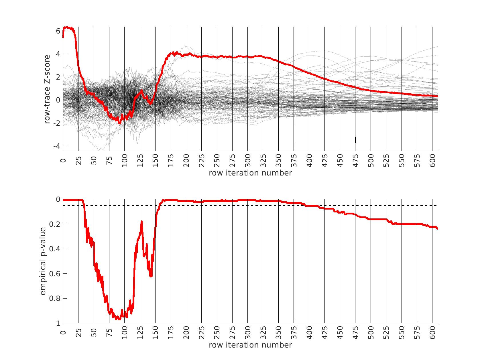
Fig 2: In this figure we show the output of the half-loop biclustering algorithm applied to the BDRN cohort in arm-1 (limited to those SNPs with maf $\geq 0.25$). As described in the main text, the algorithm proceeds iteratively, eliminating rows and columns from the case-subject-array $D$ until all have been removed. At each iteration $i$, the remaining submatrix $D(i)$ comprises case-subjects ${\cal J}(i)$ and allele-combinations ${\cal K}(i)$. At each iteration we record the ‘row-trace’ $\bar{Q}(i)$, which is the covariate-corrected average level of differential-expression between $D(i)$ and the control-subjects $X$. In the top row of subplots we show the row-trace for the data (red) as well as for $128$ label-shuffled trials (black). Each of the row-traces has been transformed into an iteration-dependent z-score (estimated using the distribution of label-shuffled trials at that iteration). In the bottom row we show the corresponding empirical p-value, as estimated for each iteration using the label-shuffled trials. The dashed black-line corresponds to the 95th percentile (i.e., a significance value of 0.05 if each iteration were considered independently). If the signal were homogeneous we would expect to see the red trace begin at a high value and decay relatively monotonically. By contrast, we see strong evidence for heterogeneity; the red trace is far from monotonic. The overall p-value for the data (red-trace), estimated using the strategy in [65], is $p\lesssim 1/64$. Note that the trace is significant over a range of iterations, including $i\in\left[175,350\right]$.

In idealized scenarios where the ‘true’ bicluster is sharply defined, the trace typically has a sharp peak near the $D(i)$ that most closely corresponds to the bicluster [64, 65]. However, in this case while the trace has a peak at around $i\sim 175$, this peak is not particularly sharp, and the trace is nearly as significant across a range of iterations $i\in[175,350]$. The largest of these submatrices (i.e., $D(175)$) corresponds to $\sim 47\%$ of the case-subjects and $\sim 31\%$ of the allele-combinations. The smallest of these submatrices (i.e., $D(350)$) corresponds to $\sim 21\%$ of the case-subjects and $\sim 9\%$ of the allele-combinations.

This ‘plateau’ of significance indicates that the true signal is not a perfectly crisp and well-delineated bicluster. Instead, this plateau suggests that, while there are certain ‘core’ case-subjects that exhibit a strong similarity across certain allele-combinations, there are additional case-subjects that are ‘adjacent’ to those in the core. These adjacent subjects exhibit a slightly weaker similarity involving a slightly expanded set of allele-combinations. Consequently, we expect iterations in the interval $i\in[175,350]$ to provide a range of approximations to the true ‘core’ signal (which is still unknown). One could certainly select the iteration with the highest training-$p$-value to approximate the bicluster, but as nearby iterations have nearly the same training-$p$-value, we expect them to also provide reasonable estimates of the true signal.

Given our approximation to the signal described above from the training-data-set, we test for replication in each of the replication-arms 2, 3 and 4. We are interested in how strongly our approximate signal replicates, as well as whether our approximation has been compromised by overfitting. Because the signal spans a range of iterations in arm-1, we assess the extent of replication across the plateau $i\in[175,350]$. This interval corresponds to significant values of the trace $\bar{Q}(i)$ as well as the AUC $A(i)$ defined only using the training-data.

Fig 3: In this figure we illustrate the replication of the bicluster in arm-2. Note that the SNP-overlap between arm-1 and arm-2 is $\sim 85\%$. On the top we show $A(i)$ in red and $A^{\prime}(i)$ in green. On the bottom we show the associated p-values for $A(i)$ and $A^{\prime}(i)$, calculated with respect to $H0$ and $H0^{\prime}$ for each iteration individually. Standard significance-levels $0.05$ and $0.01$ are shown in dashed- and dotted-lines, respectively. The interval $i\in[175,350]$ is highlighted in white. Note that both $A(i)$ and $A^{\prime}(i)$ have peaks within the range that the trace was significant (c.f. Fig 2). The overall replication for arm-2 within the interval $i\in[175,350]$ is estimated at $p\lesssim 10^{-12}$.

Fig 4: This figure is similar to Fig 3, except that we use arm-3 instead of arm-2. The overall replication for arm-3 within the interval $i\in[175,350]$ is estimated at $p\lesssim 10^{-3}$. Note that the SNP-overlap between arm-1 and arm-3 is only $\sim 50\%$.

Fig 5: This figure is similar to Fig 3, except that we use arm-4 instead of arm-2. The overall replication for arm-3 within the interval $i\in[175,350]$ is estimated at $p\lesssim 10^{-3}$. Note that the SNP-overlap between arm-1 and arm-4 is only $\sim 30\%$.

The results of this replication study for arm-2 are shown in Fig 3. The top subplot illustrates the AUC $A(i)$ (red) and $A^{\prime}(i)$ (green) as a function of $i$. The bottom subplot shows the associated $p$-value for each $i$ (under a label-shuffled null-hypothesis). Note that the training-AUC $A(i)$ is high over the range of iterations $i\in[175,350]$ for which the training-$p$ value is significant. Note also that the peak of $A(i)$ occurs within a few iterations of the peak of the training $p$-value. This correspondence corroborates the claims made above: we believe we have detected a disease-related signal within the training-data-set that involves only a subset of subjects and alleles. While the magnitude of the replication-AUC $A^{\prime}(i)$ is lower than the training-AUC $A(i)$, the value of $A^{\prime}(i)$ is also statistically significant over the range of iterations $i\in[175,350]$, with a peak at roughly the same point.

Similar results for arm-3 and arm-4 are shown in Figs 4 and 5. Note that the SNP-overlap between these arms and the training-data-set is quite a bit lower than that for arm-2. Recall that arm-2 has a overlap of $\sim 85\%$ with the SNPs in arm-1, while arm-3 and arm-4 have overlaps of $\sim 50\%$ and $\sim 30\%$, respectively.

We believe that this reduction in SNP-overlap is partially responsible for the reduction in the magnitude of replication-AUCs observed in these arms. To test this hypothesis, we randomly eliminate SNPs from arm-2 until the SNP-overlap between the training-data-set and arm-2 is equal to the SNP-overlap between the training-data-set and arm-3. The results of this replication-study are shown in Fig 11: note that the amplitude of $A^{\prime}(i)$ has degraded in comparison to the values shown in Fig 3. We then randomly eliminate even more SNPs, until the SNP-overlap between the training-data-set and arm-1 is equal to the SNP-overlap between the training-data-set and arm-4 (see Fig 12), and the amplitude $A^{\prime}(i)$ degrades even further. More generally, by reducing the number of SNPs we include in the replication-arm, we can cause the values of $A^{\prime}(i)$ to drop; depending on the subset of SNPs retained, the values of $A^{\prime}(i)$ for arm-2 can be reduced to values similar to those observed in arm-3 and arm-4.

In summary, the AUC associated with the genotype-based bicluster score discovered in the training-data-set replicates to varying degrees across all 3 replication arms. In each case the average $A^{\prime}(i)$ calculated over the interval $i\in[175,350]$ was significantly larger than what one would expect were the case- and control-labels in the replication-arm randomly permuted ($p\lesssim 1/1000$). Consequently, we are fairly certain that – while our approximation of the bicluster is far from perfect – we have indeed identified a robust disease-related signal which generalizes across a variety of different BD studies.

Interaction with covariates

Given these observations, it is natural to ask what might be driving the signal associated with this bicluster. We first checked to see if the bicluster was driven by the ancestry-related covariates in our data-set. As shown in Figs 13 and 14, the subjects in the bicluster have a distribution of ancestries similar to the remainder of arm-1 (recall that we corrected for ancestry as a covariate). By considering the subjects remaining in $D(i)$, we also determined that the bicluster does not seem to be associated with sex (see Fig 15).

Interaction with BD subtype

We then checked to see if the bicluster was associated with bipolar subtype. We measured the fraction of subjects classified as bipolar-type-1 versus bipolar-type-2 as our algorithm proceeded. Specifically, we measured the fraction of case-subjects in ${\cal J}(i)$ that were classified as BDI and BDII. If the bicluster were driven by BDII subjects, then we would expect the proportion of remaining BDII case-subjects to increase with the iteration-index $i$. Conversely, if the bicluster were driven by BDI subjects, then we would expect the proportion of remaining BDI case-subjects to increase with iteration-index. As shown in Fig 6, we found that this latter scenario holds; the bicluster was significantly enriched for BDI relative to BDII. This enrichment for BDI also impacts our risk-prediction results (see below). Note that, when determining this enrichment, we compare the proportion of BDI and BDII case-subjects at each iteration to the proportion at iteration $i=1$ (i.e., across all case-subjects in arm-1). In this manner our enrichment is defined relative to the starting proportion of BDI and BDII subjects in our training-arm, and is not influenced by the recruitment rates for BDI and BDII (which can differ across studies).

While significant, this BDI-enrichment was not completely overwhelming: the initial fraction of BDII participants in arm-1 was $\sim 31\%$, which dropped to $\sim 26\%$ at iteration $i=240$. Thus, while the majority of the case-subjects in the bicluster are classified as BDI, those classified with BDII do still contribute to the overall signal. It is possible that this BDI-enrichment is due to a true difference between the BD-subtypes at the genetic level. However, it is also possible that this enrichment is partially driven by inaccuracies associated with classification [14].

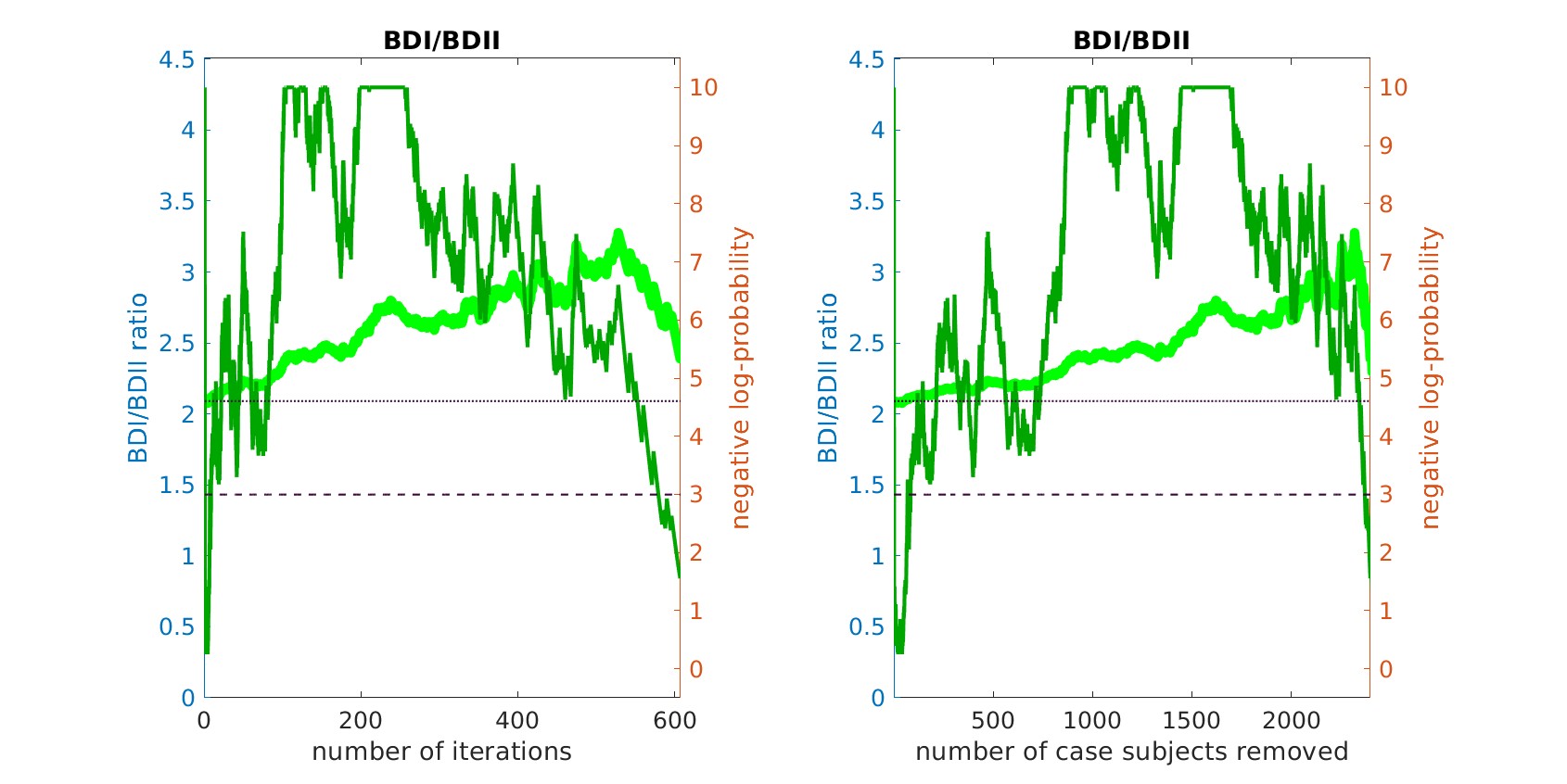
Fig 6: This figure plots the ratio of BDI to BDII subjects within ${\cal J}(i)$ (light-green, left y-axis) as a function of the iteration $i$ (left) and the number of removed case-subjects (right). The dark-green line corresponds to the negative-log-probability (right y-axis) of observing a ratio at least as large by chance. The dashed and dotted horizontal lines indicate $0.05$ and $0.01$ significance values, respectively. Note that the BDI population is over-represented across a range of iterations including $i\in[175,350]$, implying that the bicluster we observe is significantly enriched for BDI subjects.

Bicluster-informed PRS Performance

As described in the Methods section, we calculated the population-wide ${\bf PRS_{\text{\footnotesize wide}}}(j^{\prime};\tilde{p})$ and the bicluster-informed ${\bf PRS_{\text{\footnotesize bicl}}}(j^{\prime};i,\tilde{p})$ across a variety of iterations $i$ and $\tilde{p}$-thresholds. We compared the bicluster-informed ${\bf PRS_{\text{\footnotesize bicl}}}(j^{\prime};i,\tilde{p})$ performance to the one generated by the population-wide ${\bf PRS_{\text{\footnotesize wide}}}(j^{\prime};\tilde{p})$ across a variety of $\tilde{p}$-thresholds. Results for arm-2 are shown in Fig 7. Results for arm-3 and arm-4 are shown alongside arm-2 in Fig 8, and individually in Figs 21 and 22.

Note that, when constructing ${\bf PRS_{\text{\footnotesize bicl}}}(j^{\prime};i,\tilde{p})$, we restrict ourselves to a subset of case-subjects within the training-arm determined by ${\cal J}(i)$. In this case, when $i\in[175,350]$ the case-subset ${\cal J}(i)$ retains only $\sim 50\%-20\%$ of the original case-subjects in arm-1. Typically, one might expect a reduction in the number of case-subjects to yield a corresponding reduction in power, giving rise to a reduced discriminability in the testing-arms 2,3 and 4. However, as we see in Fig 8, the discriminability for ${\bf PRS_{\text{\footnotesize bicl}}}(j^{\prime};i,\tilde{p})$ is typically higher than ${\bf PRS_{\text{\footnotesize wide}}}(j^{\prime},\tilde{p})$ when $i\in[175,350]$. This suggests that the case-subjects in ${\cal J}(i)$ identified by the bicluster correspond to a stronger genetic signal, likely arising from the increased homogeneity within ${\cal J}(i)$.

Note that ${\bf PRS_{\text{\footnotesize bicl}}}$ and ${\bf PRS_{\text{\footnotesize wide}}}$ are not capturing identical signals (see the Nagelkerke $R^{2}$ analysis in the Supporting information). It is useful to compare the performance of ${\bf PRS_{\text{\footnotesize bicl}}}$ with ${\bf PRS_{\text{\footnotesize wide}}}$ as there are features of ${\bf PRS_{\text{\footnotesize bicl}}}$ which indicate that it is more robust than ${\bf PRS_{\text{\footnotesize wide}}}$. As one example, we point out that ${\bf AUC_{\text{\footnotesize bicl}}}(i,\tilde{p})$ is markedly higher than ${\bf AUC_{\text{\footnotesize wide}}}(\tilde{p})$ when the number of SNPs used (denoted by ${N_{\text{\footnotesize SNP}}}$) is fewer; one begins to see the effect between $1K$ and $10K$. This suggests that the bicluster-informed ${\bf PRS_{\text{\footnotesize bicl}}}(j^{\prime};i,\tilde{p})$ is not only outperforming the population-wide ${\bf PRS_{\text{\footnotesize wide}}}(j^{\prime};\tilde{p})$, but also correctly attributing the largest PRS-weights to those SNPs that truly carry the signal (and which are most important for replication). As one illustration, by comparing the values of ${\bf AUC_{\text{\footnotesize bicl}}}$ to ${\bf AUC_{\text{\footnotesize wide}}}$ in Fig 8, we can directly see that the bicluster-informed PRS would replicate across arms 2,3 and 4 for values of $i=225$ and ${N_{\text{\footnotesize SNP}}}\in[10^{3},10^{4}]$, while the population-wide PRS would not.

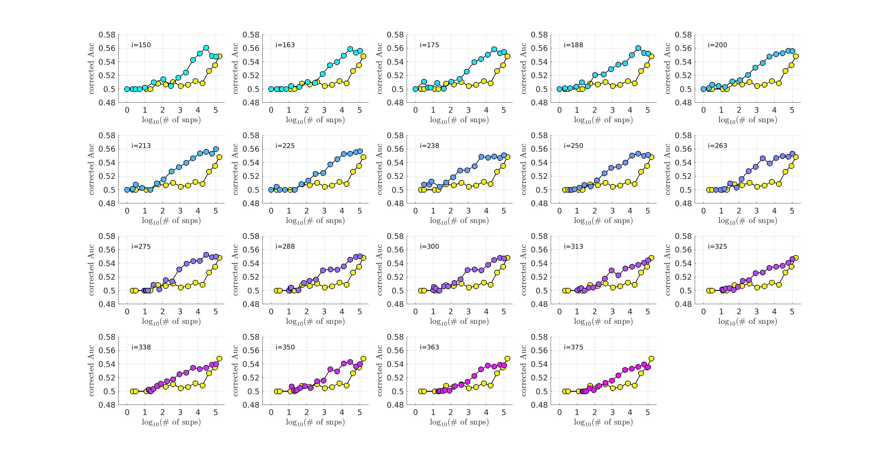
Fig 7: In each subplot we show in yellow the ${\bf AUC_{\text{\footnotesize wide}}}^{\prime}(\tilde{p})$ (vertical) for arm-2 as a function of the number of SNPs corresponding to each $\tilde{p}$-threshold (horizontal, log-scale). Additionally, we show ${\bf AUC_{\text{\footnotesize bicl}}}^{\prime}(i,\tilde{p})$ for a particular iteration $i$ (with $i$ varying across subplots). The color-code used for ${\bf AUC_{\text{\footnotesize bicl}}}^{\prime}(i,\tilde{p})$ ranges from blue to pink, corresponding to the iteration index $i$. Note that, by using the bicluster to inform the PRS, the performance typically improves. This improvement in performance becomes marked when the number of SNPs is limited to a relatively small fraction of the total (e.g., $\sim 1\%$ of the total, corresponding to a $\log_{10}(\#)$ of $\sim 3$).

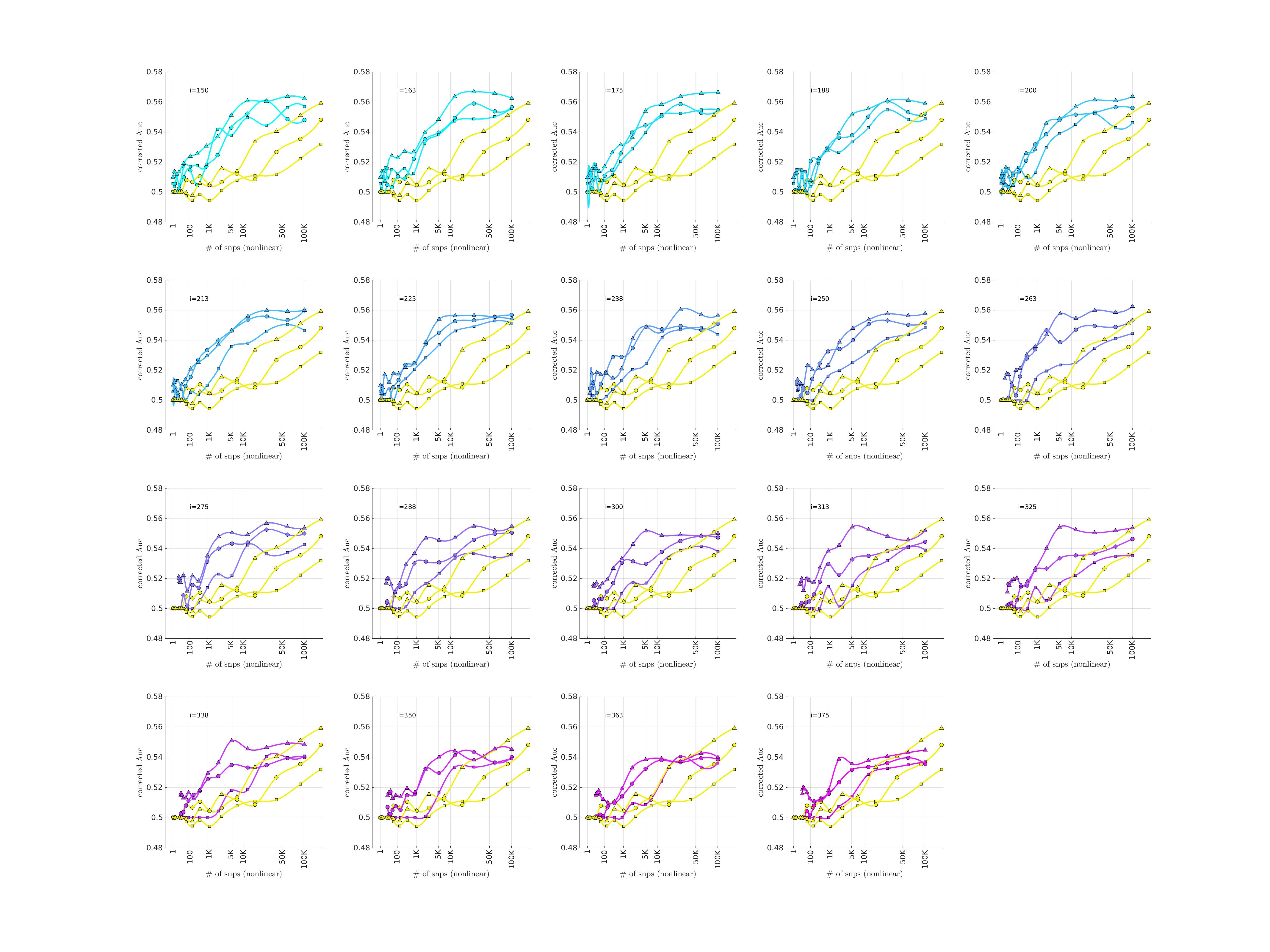
Fig 8: This figure uses circles to displays the same information as Fig 7 (corresponding to replication arm-2). In this figure we use an algebraic-scale for the horizontal-axis (rather than a log-scale) in order to better emphasize the interval where the number of SNPs used is between $1K$ and $10K$. The results for replication arm-3 and arm-4 are shown using squares and triangles, respectively.

Motivated by the significant BDI-enrichment seen within the training-arm (see Fig 6), we repeated these assessments for the BDI- and BDII-populations within the testing-arms. The results are shown in Figs 9 and 10, respectively. Note that the improvement to risk-prediction persists for the BDI-population, but is not as robust for the BDII-population. The performance of ${\bf AUC_{\text{\footnotesize bicl}}}^{\prime}(i,\tilde{p})$ is particularly poor for the BDII-population in arm-3, for which there were only $M=435$ BDII-subjects (i.e., the fewest out of all the arms). It is possible that the variation in the performance of ${\bf AUC_{\text{\footnotesize bicl}}}^{\prime}(i,\tilde{p})$ for the BDII-population across the replication-arms has to do with these differences in power. It is also possible that there are other systematic issues affecting the BDII-population, including variation in the life history of the subjects or the metrics used for their clinical diagnosis [14].

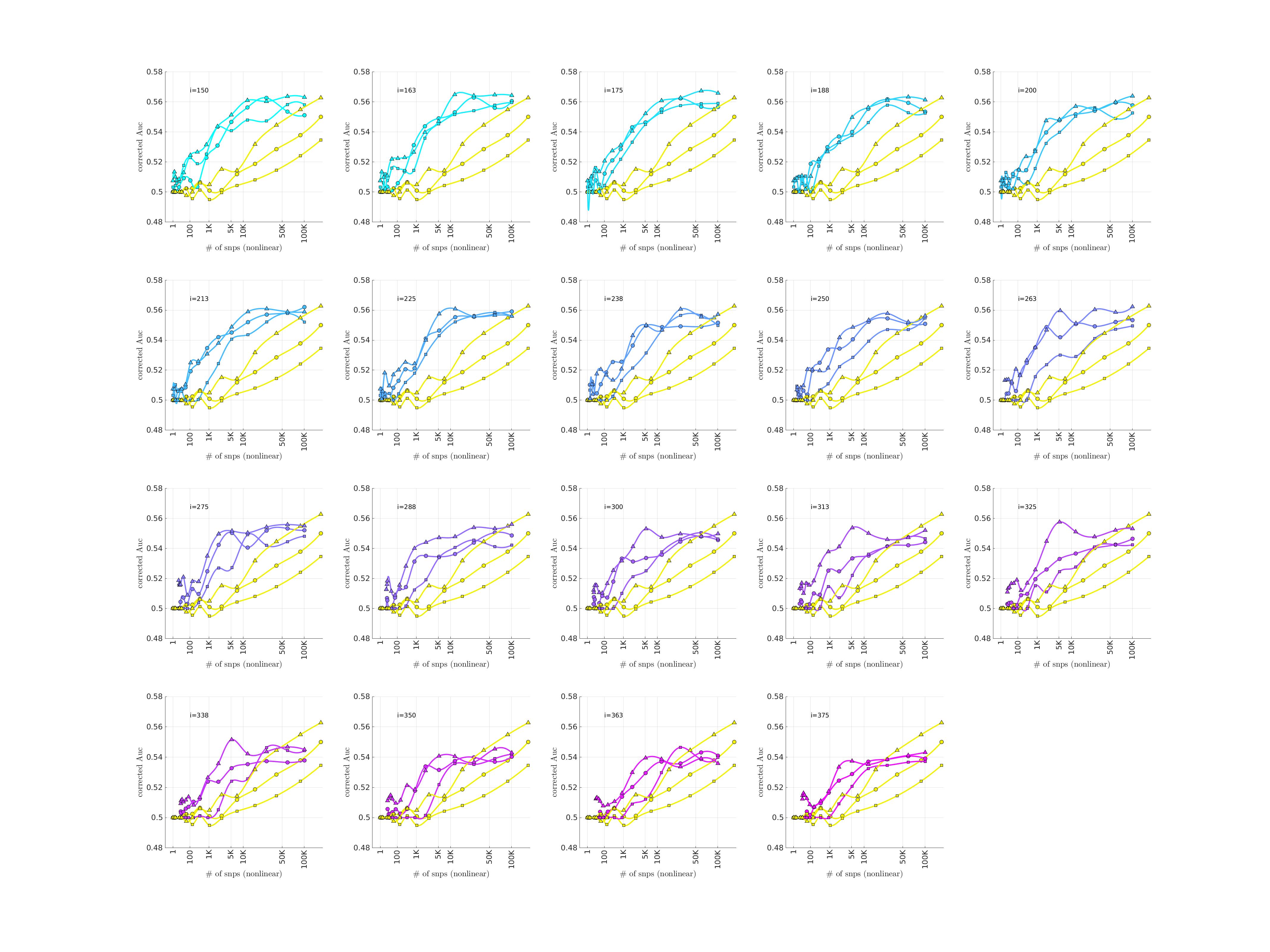
Fig 9: This figure is similar to Fig 8, except that we limit ourselves only to those case-subjects in the replication-arms which are classified as BDI. This subset corresponded to $66\%$ ($M=3834$), $84\%$ ($M=2995$) and $75\%$ (M=5107) of the case-population for arms 2, 3 and 4, respectively. For reference the training-arm had $M=1645$ BDI case-subjects, corresponding to $65\%$ of the case-population in arm-1.

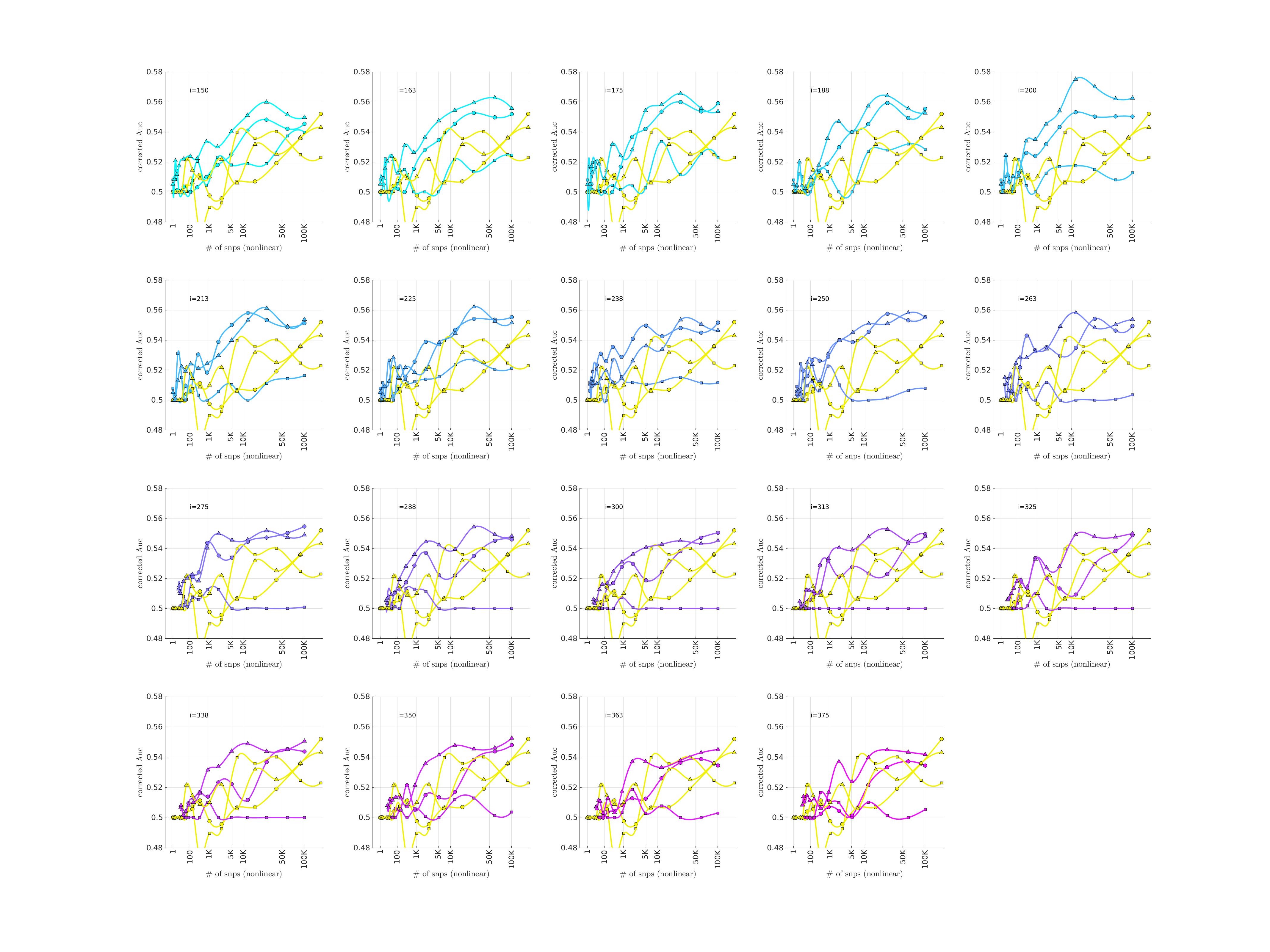
Fig 10: This figure is similar to Fig 8, except that we limit ourselves only to those case-subjects in the replication-arms which are classified as BDII. This subset corresponded to $19\%$ ($M=1082$), $12\%$ ($M=435$) and $16\%$ (M=1060) of the case-population for arms 2, 3 and 4, respectively. For reference the training-arm had $M=788$ BDII case-subjects, corresponding to $31\%$ of the case-population in arm-1.

Gene-enrichment: 

We also perform a simple over-representation analysis, measuring the overlap $\kappa(i,l)$ between the bicluster $D(i)$ at iteration $i$ and the various neuronally-related pathways ${\cal H}_{l}$ from the go_bp ontology (see Methods). The average z-score for the enrichment-values $\kappa(i,l)$, averaged over the interval $i\in[175,350]$ and all neuronally-related pathways, is quite significant, with $p\lesssim 1e-4$ (as determined by a permutation-test). Examples of some of the more significantly over-represented pathways are shown in Table 1.

annotation	175	200	225	250	275	300	325	350	375
synaptic vesicle endocytosis	3.49	2.10	1.28	1.94	0.22	0.24	0.24	0.26	0.26
positive regulation of neurogenesis	3.29	2.36	0.36	0.39	0.75	0.08	0.11	0.13	0.15
neurological system process involved in regulation	3.10	2.88	2.10	1.07	1.46	1.74	0.21	0.22	0.23
positive regulation of neuroblast proliferation	2.97	0.71	0.18	0.20	0.22	0.23	0.24	0.26	0.30
neurological system process	2.94	1.10	1.78	2.14	1.11	0.84	0.43	0.98	1.20
synaptic vesicle exocytosis	2.86	3.03	3.62	4.31	2.22	0.17	0.19	0.19	0.19
regulation of neurogenesis	2.81	1.57	0.85	0.60	0.96	0.36	0.68	0.53	0.89
establishment of synaptic vesicle localization	2.78	2.03	2.70	3.66	1.85	0.15	0.17	0.18	0.18
synaptic vesicle localization	2.78	2.03	2.70	3.66	1.85	0.15	0.17	0.18	0.18
synaptic vesicle transport	2.78	2.03	2.70	3.66	1.85	0.15	0.17	0.18	0.18
positive regulation of neuron differentiation	2.63	0.99	0.47	0.34	0.54	0.87	1.27	0.16	0.20
axonogenesis	2.53	1.83	2.41	1.03	1.73	1.30	1.03	1.03	0.85
cell morphogenesis involved in neuron differentiat	2.52	2.18	3.19	1.44	2.42	1.67	1.45	1.53	1.51
generation of neurons	2.31	1.98	2.54	1.46	2.06	1.07	0.98	1.06	1.36
axon development	2.25	1.70	2.29	0.99	1.68	1.26	0.99	1.00	0.83
positive regulation of axonogenesis	2.17	3.36	0.64	0.43	0.64	0.13	0.15	0.18	0.19
axonal fasciculation	2.07	0.17	0.21	0.24	0.30	0.30	0.30	0.30	0.30
neuron development	2.04	1.73	2.73	2.08	2.62	1.32	0.95	1.25	1.30
central nervous system projection neuron axonogene	2.04	1.76	2.94	0.16	0.20	0.21	0.23	0.25	0.25
neurogenesis	2.01	1.64	2.38	1.57	2.42	0.90	0.86	0.92	1.16
neuron projection morphogenesis	1.91	1.53	2.23	1.13	1.96	1.18	0.92	0.90	0.72
central nervous system neuron axonogenesis	1.88	1.85	3.40	0.12	0.16	0.17	0.19	0.22	0.23
neurotransmitter uptake	1.87	0.41	0.12	0.15	0.17	0.18	0.20	0.22	0.24
neuron projection development	1.81	1.17	2.33	1.57	1.84	1.02	0.90	1.02	0.93
axon guidance	1.81	0.83	1.64	1.11	1.63	2.05	2.18	1.80	1.58
neuron projection guidance	1.81	0.83	1.64	1.11	1.63	2.05	2.18	1.80	1.58
synapsis	1.69	1.04	1.97	3.19	0.18	0.20	0.23	0.24	0.25
synaptic transmission	1.64	0.51	0.40	0.77	0.44	0.26	0.31	0.59	0.44
regulation of neurological system process	1.63	0.90	1.06	1.37	0.53	0.45	0.78	1.06	0.56
neuron differentiation	1.59	1.40	2.04	1.73	2.20	1.34	1.21	1.25	1.53
positive regulation of neurological system process	1.48	0.61	0.67	0.46	0.11	0.13	0.17	0.19	0.20

Table 1: Here we list some of the pathways from the go_bp ontology. Shown here are only the 32 most significant pathways as determined by $\kappa(175,l)$. Each pathway is listed alongside approximations to its individual over-representation p-value (estimated using the hypergeometric-distribution). The $-\log_{10}(p)$-values are listed for iterations $175$-$350$ (see top row). Those annotations with an individual over-representation p-value smaller than $0.05$ are marked in red.

Secondary bicluster: 

After discovering and analyzing the primary bicluster within arm-1 (described above), we searched for a secondary bicluster. We first eliminated the structure associated with the primary bicluster by scrambling the entries of the submatrix $D(175)$ (see [65] for details). We then reran our half-loop algorithm on this scrambled version of arm-1. While we did find a secondary trace that was indicative of heterogeneity, the overall level of differential-expression was far lower than for the first bicluster (see Fig 23). Moreover, the structure associated with this secondary trace did not significantly replicate (see Figs 24 – 26). It is possible that a secondary bicluster exists, but that we could not pinpoint it due to a lack of power in our training-arm. It is also possible that the scrambled version of arm-1 is heterogeneous, but not in a way that can be described by a bicluster (see [65] for examples along these lines). In either case, a larger sample size will be required to further probe this residual heterogeneity.

Control biclusters: 

Up to this point we have only considered biclusters within the case-population; i.e., subsets of case-subjects which exhibit a genetic-signature that is not shared by the control-subjects. It is natural to ask if there are also biclusters that exist within the control-population (i.e., whether or not the control-population is homogeneous). Such ‘control-biclusters’ might be induced by batch effects or issues associated with recruitment; e.g., many of the BD controls may be drawn from another disease study (such as cancer), thus being more likely to share certain genetic features. It might also be the case that some of the control-biclusters are biologically significant, corresponding to mechanisms which protect against the disease. In either scenario, a better understanding of the heterogeneity within the control-population can assist in designing homogeneous populations of controls for future studies.

We can easily carry out this analysis simply by reversing the labels within our biclustering algorithm (i.e., swapping $D$ and $X$). This reversed search will find biclusters that are driven by genetic-signatures which are more prevalent within the controls than within the cases. As mentioned above, we find that the control-population within arm-1 is quite homogeneous: the trace decays monotonically with no distinguished peaks (see Fig 27). This homogeneity can be viewed as a validation of our initial choice of arm-1 as a training- or discovery-arm.

On the other hand, we find strong evidence for heterogeneity within the control-populations of arms 2, 3 and 4 (see Figs 28-30). In each case the trace has a significant distinguished maximum involving only a fraction of the control-subjects (i.e,. $13\%$, $28\%$ and $15\%$ of the controls, respectively).

The heterogeneity observed in the control-populations of arms 2, 3 and 4 might be expected; each of these arms comprises multiple smaller studies. Notably however, the ‘control-biclusters’ within these arms cannot all be easily dismissed as batch-effects. Indeed, each of the dominant control-biclusters is also quite significant, while also usually well balanced across the ancestry-related covariates and individual cohorts within each arm. Each of these dominant control-biclusters also replicates across the majority of other arms.

Thus, while a portion of these control-biclusters might be driven by batch-effects or other idiosyncrasies in the control-population, it is possible that that some of these signals have biological relevance, perhaps involving mechanisms which protect against BD (as the control-biclusters were identified specifically because they involved genetic patterns not as prevalent across the cases). Consequently, we would recommend considering this heterogeneity when performing other kinds of analysis. For example, one should not necessarily assume that the controls are homogeneous, as small subgroups of controls can likely exhibit genetic-signatures that are distinct from the rest.

Discussion

In this paper we have taken a ‘genotype-driven’ approach to investigating genotypic-heterogeneity. That is to say, first we used only basic phenotypic classification to divide subjects into cases (BD) and controls (not BD). We then applied a biclustering analysis to identify genetic subgroups within the case-population. Analyzing the BDI and BDII cases as a group allowed us to identify the shared signal delineating a bicluster (described above). This shared signal was driven by a genetically homogeneous subset of the cases, which can then be used to inform a more robust PRS with better replication across studies.

This PRS-study suggests two hypotheses for future work: First, that the bicluster found in the training-arm indeed represents a subset of case-subjects exhibiting a homogeneous genetic subtype of BD (consistent with the replication-study shown in Figs 3, 4 and 5). Second, by isolating homogeneous subsets of case-subjects, more robust PRSs can be constructed, with the potential of improving SNP-replication in BD GWAS and, ultimately, better understanding the etiology of Bipolar Disorder.

In some respects our approach can be termed ‘unsupervised’, as we did not use BD-subtype (BDI vs. BDII) or subphenotype information to guide our primary analysis. This unsupervised approach allows us to circumvent many of the challenges associated with phenotype classification, such as missingness and variation in assessment and collection process (e.g., expert-led vs. self-report). It also allows us to identify genetic patterns which straddle traditional classifications provided the signature is not present in the control group. E.g., though our bicluster was enriched for BDI, it was by no means limited to BDI and included many BDII cases.

Along these lines, we believe that a similar unsupervised approach could be used to search for interactions between the signals we have found and other diseases, as well as for cross-psychiatric-disorder signals not present in the control group. There are many examples of genetic interactions along these lines: the SNPs driving BD have a strong correlation with those driving schizophrenia, and also share overlap with the SNPs driving MDD, OCD, anorexia nervosa, ADHD, ASD and substance-abuse [72, 34, 73]. Many SNPs have also been associated with other disorders [74, 75, 17, 76]. More generally speaking, BD shows substantial overlap with other disorders; e.g., more than $90\%$ of BD subjects exhibit lifetime comorbidity [3] with at least one other psychiatric disorder [77, 78, 58], or non-psychiatric disorder [79, 80, 81]. This high rate of comorbidity implies that BD is one of multiple disorders which perturb several important regulatory systems [82, 83]. Given these relationships, it is possible that the bicluster-score and/or the bicluster-limited PRSs may also correlate with some of the signals of these other disorders. It is possible that we could discover interesting biclusters which cross psychiatric disorders or are present in the control groups and predict resistance to psychiatric illness more generally; we defer an investigation of these interactions to future work.

The biclustering algorithm we use also offers a ’supervised’ option which uses additional information (e.g., BD-subtype or other clinical data) to subdivide the case-population while searching for heterogeneity. sex might be one important variable to include in such a supervised BD analysis. For example, while most studies do not indicate large difference in BD prevalence between men and women (indeed, the bicluster we identified was not significantly enriched for sex), there is some evidence of a sex disparity in the prevalence of BDII, rapid-cycling and mixed-episodes [84, 85]. Age may also be an important role-player, as an earlier age of onset may be associated with higher severity and a poorer long-term prognosis (possibly due to mis-diagnoses at an early stage) [86, 57].

One limitation of our current study is that it is restricted to common variants (i.e., SNPs with a high minor-allele-frequency). While it is encouraging that the common variants alone can be used to find replicable and robust signals, it is also likely that the rare variants also play a role in the heterogeneity of BD. Analyzing the rare variants brings new challenges, as rare variants often require more statistical power to detected and/or validate [87, 88, 89, 90, 91, 92].

Another more serious limitation is that our training-arm is quite restricted in terms of ancestry. More generally, almost all the individuals in our data-set are of European descent. We expect that this lack of diversity will limit our ability to pinpoint the most biologically relevant signals, as many previous GWAS analyses have not generalized well to cohorts of different ancestry [93, 94, 95, 96, 97, 29]. An important future direction will be to investigate the interactions between genotypic heterogeneity and ancestry.

We do not expect a full analysis of genetic-heterogeneity to be entirely trivial. For example, appropriately correcting for ancestry is not always easy, even when searching for homogeneous signals. When searching for heterogeneity such a correction becomes more complicated and, necessarily, involves more parameters. Larger (and more diverse) sample sizes will likely be necessary to clarify the genetic- and phenotypic subtypes of BD, as well as the interaction between these subtypes and ancestry. We suspect that a careful treatment of the associated statistical issues will pose a significant challenge. Nevertheless, these advancements will likely further improve our understanding of the etiology of BD.

Supporting information

Additional replication analyses in arm-2

Figs 11 and 12 illustrate the replication obsreved in arm-2 when the SNP-overlap between arm-1 and arm-2 is artificially decreased.

Fig 11: This figure is similar to Fig 3, except that we randomly eliminate SNPs from arm-2 until the SNP-overlap between arm-2 and the training-arm is equal to the SNP-overlap between arm-3 and the training-arm.

Fig 12: This figure is similar to Fig 3, except that we randomly eliminate SNPs from arm-2 until the SNP-overlap between arm-2 and the training-arm is equal to the SNP-overlap between arm-4 and the training-arm.

Influence of covariates on the bicluster

Figs 13 and 14 illustrate the association between the bicluster found in arm-1 and the ancestry-related covariates. Fig. 15 illustrates the association with sex.

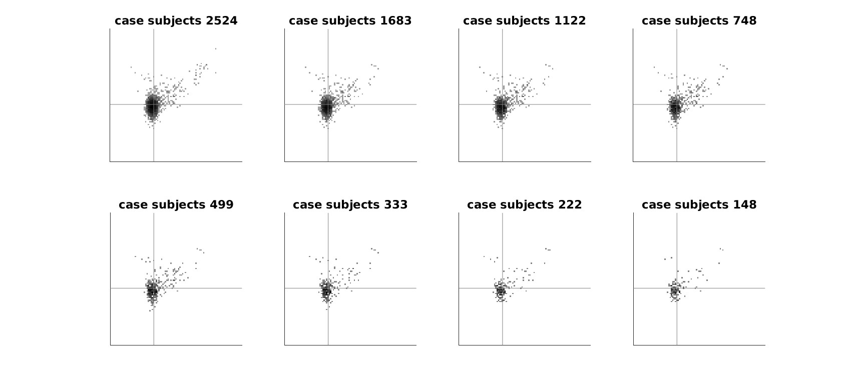
Fig 13: This figure illustrates the distribution of ancestry-associated principal-components $U^{1}_{1}$ and $U^{1}_{2}$ amongst the remaining case-subjects as the half-loop algorithm proceeds (specifically, at iterations $i\in\{96,189,276,359,442,511,585\}$). Each subplot displays a scatterplot of remaining case-subjects plotted with respect to $U^{1}_{1}$ and $U^{1}_{2}$. The number of remaining case-subjects is shown above each subplot. Note that the overall shape of the distribution does not change much as the algorithm proceeds.

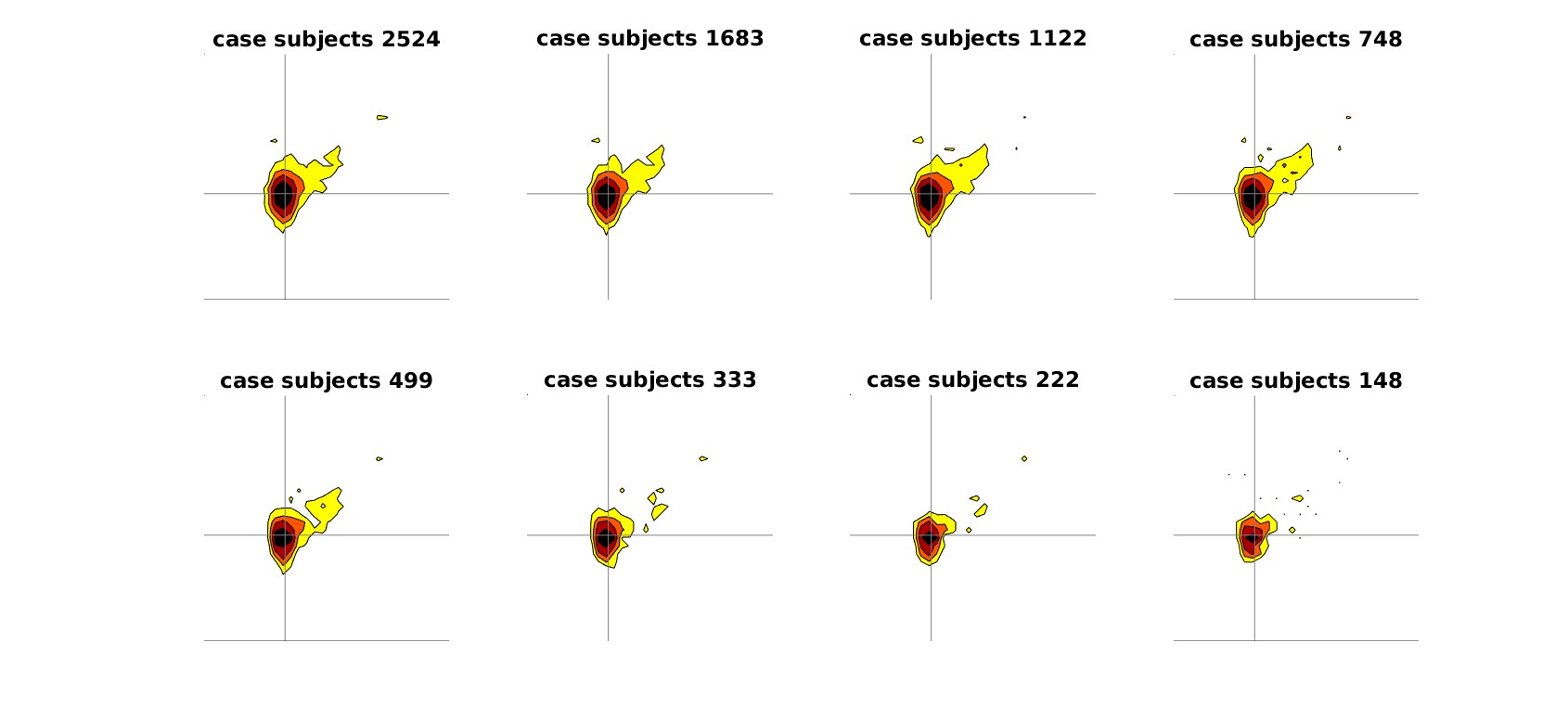
Fig 14: This figure is similar to Fig 13, except that a heat-map of the distribution is shown (rather than a scatterplot). The colors in the heat-map correspond to the logarithm of the density in the underlying distribution. Four different contours are shown, ranging from yellow to maroon, corresponding to the $20\%$, $40\%$, $60\%$ and $80\%$ percentiles of the log-density.

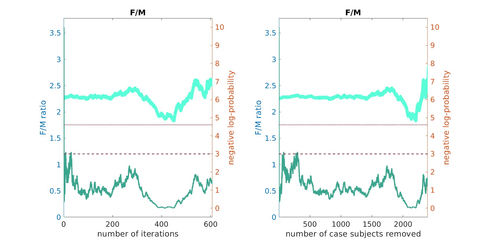
Fig 15: This figure plots the ratio of female to male subjects within ${\cal J}(i)$ (light-teal, left y-axis) as a function of the iteration $i$ (left) and the number of remaining case-subjects (right). The dark-teal line corresponds to the negative-log-probability (right y-axis) of observing a ratio at least as large by chance. The dashed and dotted horizontal lines indicate $0.05$ and $0.01$ significance values, respectively. Note that the female population is not over-represented across the range of iterations including $i\in[175,350]$, implying that the bicluster we observe is not significantly enriched for female subjects.

Interaction between bicluster-score and population-wide PRS

As described in the Methods section, we calculated the population-wide ${\bf PRS_{\text{\footnotesize wide}}}(j^{\prime};\tilde{p})$ and the bicluster-informed ${\bf PRS_{\text{\footnotesize bicl}}}(j^{\prime};i,\tilde{p})$ across a variety of iterations $i$ and $\tilde{p}$-thresholds. In Fig 16 we illustrate the correspondence between the population-wide ${\bf PRS_{\text{\footnotesize wide}}}(j^{\prime};\tilde{p})$ and bicluster-score $u^{\prime}_{j^{\prime}}(i)$ for arm-2 at $i=175$. This trend persists for other iterations, as illustrated in Figs 17 and 18.

Fig 16: In this figure we illustrate the correspondence between the population-wide ${\bf PRS}(j^{\prime};\tilde{p})$ and bicluster-score $u^{\prime}_{j^{\prime}}(i)$ for arm-2 at $i=175$. Each subplot visualizes the distribution of subjects in arm-2 as a function of bicluster-score $u^{\prime}_{j^{\prime}}(i)$ (horizontal) and ${\bf PRS_{\text{\footnotesize wide}}}(j^{\prime};\tilde{p})$ (vertical), with the SNP-$p$-value threshold $\tilde{p}$ varying across the subplots. In each subplot a heatmap is shown, representing the difference between the density of cases and controls. The color pink corresponds to areas with a higher case-density than control-density, while blue corresponds to areas with a higher control-density than case-density. The colorbar (upper-left) ranges across $\pm 25\%$ of the maximum density (taken across both the case- and control-distributions). Note that, while the bicluster-score is correlated with the population-wide PRS when $\tilde{p}$ is sufficiently high, the correlation is far from perfect. Note that, when $\tilde{p}$ is high (i.e., $\tilde{p}\sim 1$ and all the SNPs are used to generate the PRS), there is a marked correlation between case-control status and high-values of ${\bf PRS_{\text{\footnotesize wide}}}(j^{\prime};\tilde{p})$ and bicluster-score $u^{\prime}_{j^{\prime}}(i)$. However, for lower values of $\tilde{p}$ this structure shifts, and ${\bf PRS_{\text{\footnotesize wide}}}(j^{\prime};\tilde{p})$ is no longer a useful indicator of case-control status while the bicluster-score $u^{\prime}_{j^{\prime}}(i)$ is still a useful indicator. This trend persists for other iterations, as illustrated in Figs 17 and 18.

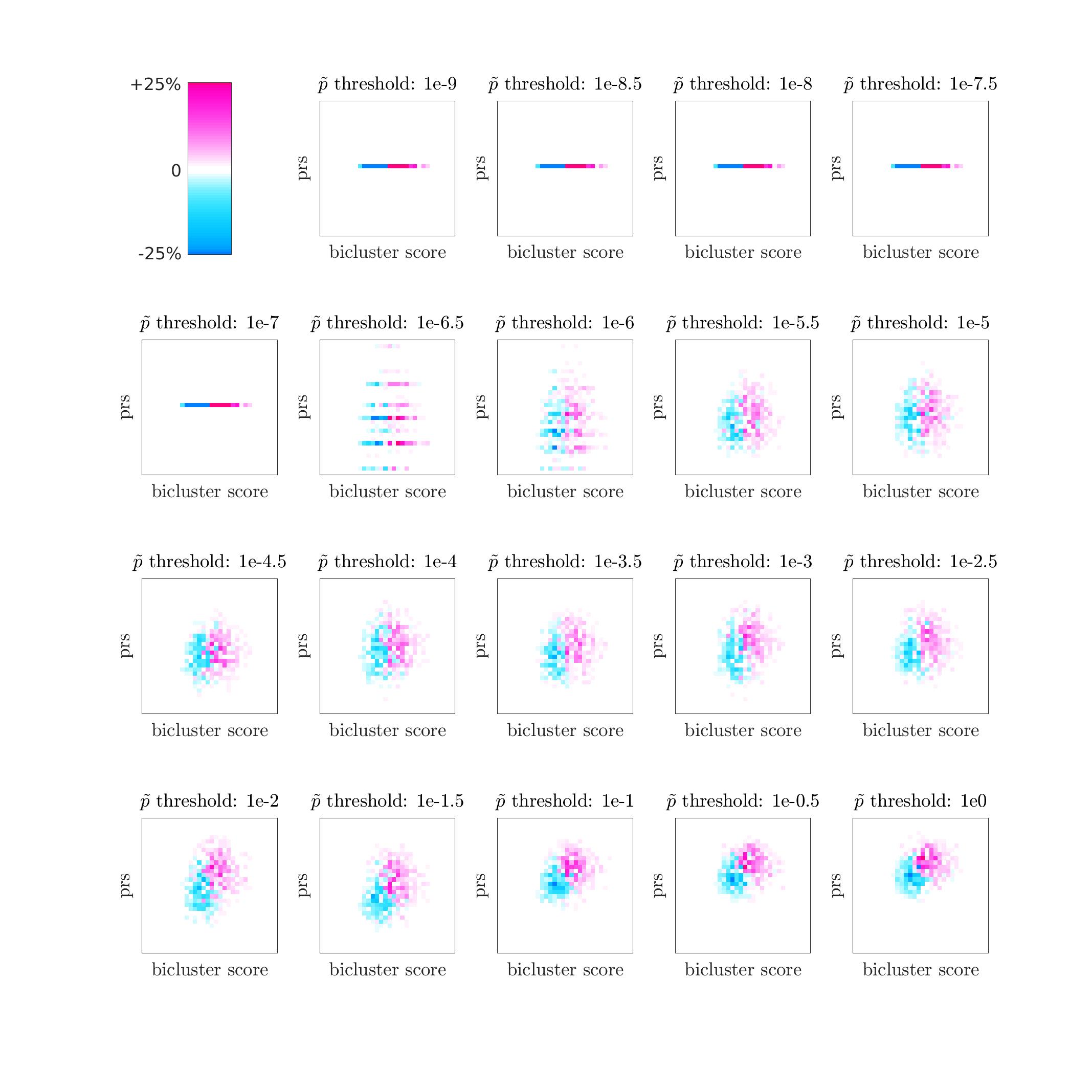
Fig 17: This figure is analogous to Fig 16, except for $i=225$.

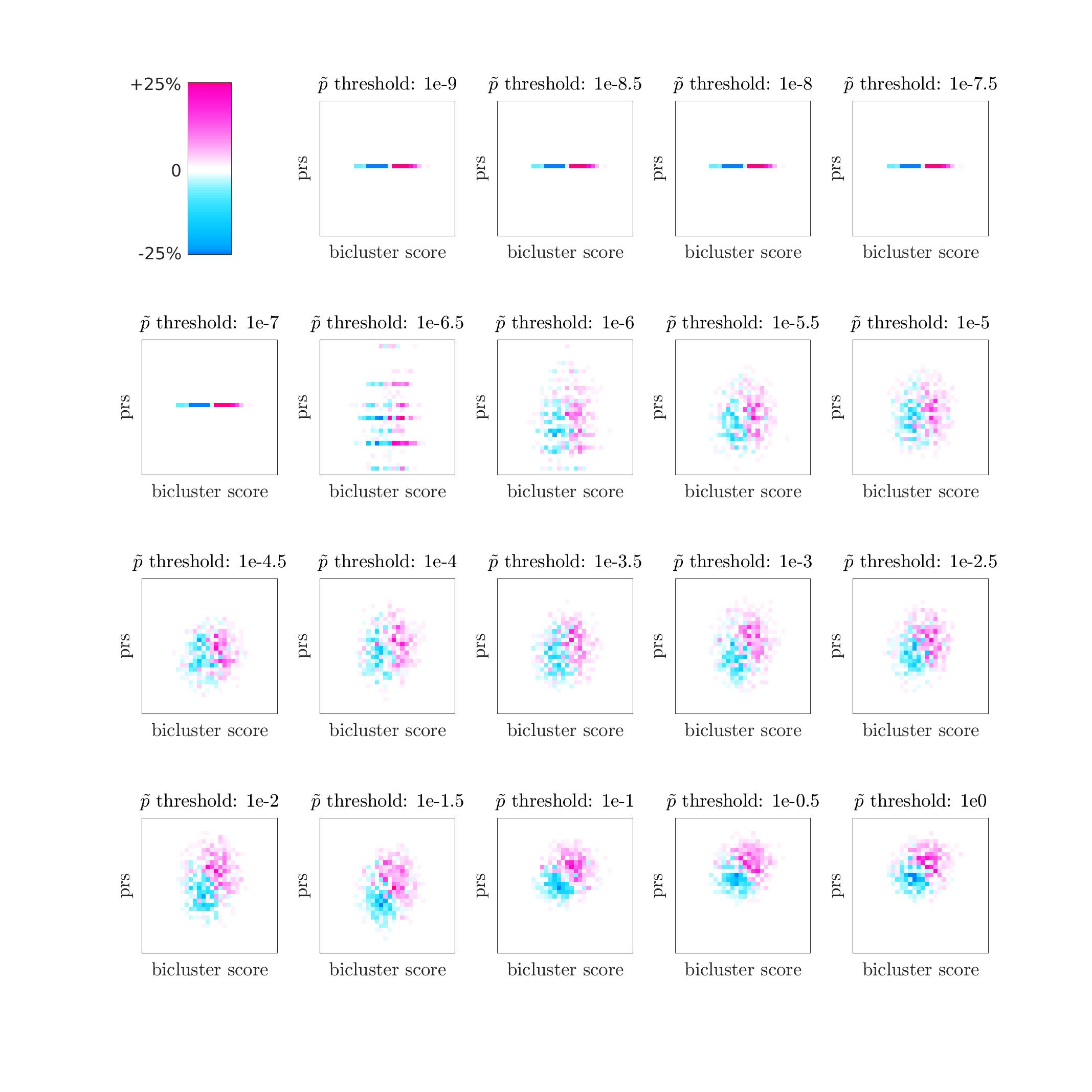
Fig 18: This figure is analogous to Fig 16, except for $i=350$.

Nagelkerke $R^{2}$ for a series of linear-models

To complement the observations of Figs 16, 17 and 18, we investigate how the bicluster-informed PRSs and the bicluster-scores themselves contribute to risk-prediction. For a given $i$ and $\tilde{p}$ we build a series of linear-models to predict case-control status. These linear-models use: (i) the ancestry-related covariates, (ii) the population-wide ${\bf PRS_{\text{\footnotesize wide}}}(j^{\prime};\tilde{p})$, (iii) the bicluster-informed ${\bf PRS_{\text{\footnotesize bicl}}}(j^{\prime};i,\tilde{p})$, and (iv) the bicluster-score $u^{\prime}_{j^{\prime}}(i)$.

The series of linear-models we consider involve successively more and more of these terms. Thus, the null linear-model attempts to predict case-control status using no terms at all (i.e., using only the average prevalence of cases and controls). The first linear-model attempts to predict case-control status using only term (i), that is, only the ancestry-related covariates. The second linear-model uses both term (i) and (ii), i.e., both the ancestry-related covariates and the population-wide PRS. The third linear-model uses terms (i), (ii) and (iii). And finally, the fourth linear-model uses terms (i)-(iv). For each linear-model we measure the Nagelkerke pseudo-$r^{2}$ value between that model and the null model The difference in pseudo-$r^{2}$ values gives an estimate of the additional explanatory power provided by each term in succession.

Results for various $i$ and $\tilde{p}$ are shown in Figs 19 and 20. Each vertical bar in this figure corresponds to a particular $i$ and $\tilde{p}$. Each vertical bar is further divided into segments illustrating the incremental Nagelkerke pseudo-$r^{2}$ value associated with each term. Note that the bicluster-informed PRS, as well as the bicluster-score $u^{\prime}_{j^{\prime}}(i)$ add explanatory power to the underlying linear model. This phenomena is most pronounced when $i$ is in the middle of the range $i\in[175,350]$ and the threshold $\tilde{p}$ is small.

The observations in Figs 16-20 suggest that the bicluster might contain information useful for improving risk-prediction. Moroever, the peak in overall $R^{2}$ when $\tilde{p}\sim 1e-2$ suggests that the signal in our bicluster-score involves subsets of SNPs which do not individually achieve genome-wide significance.

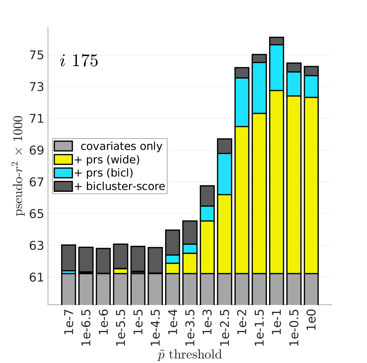
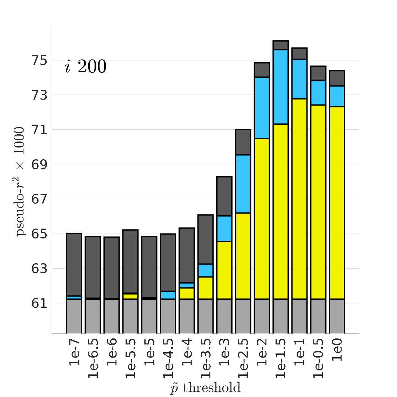
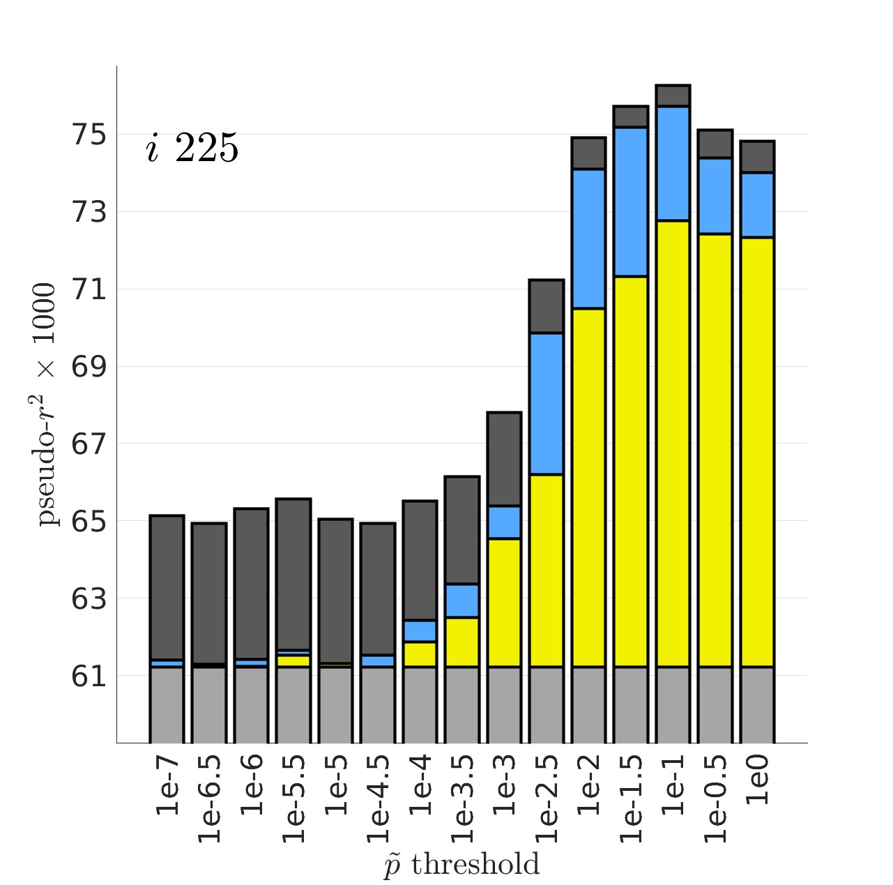
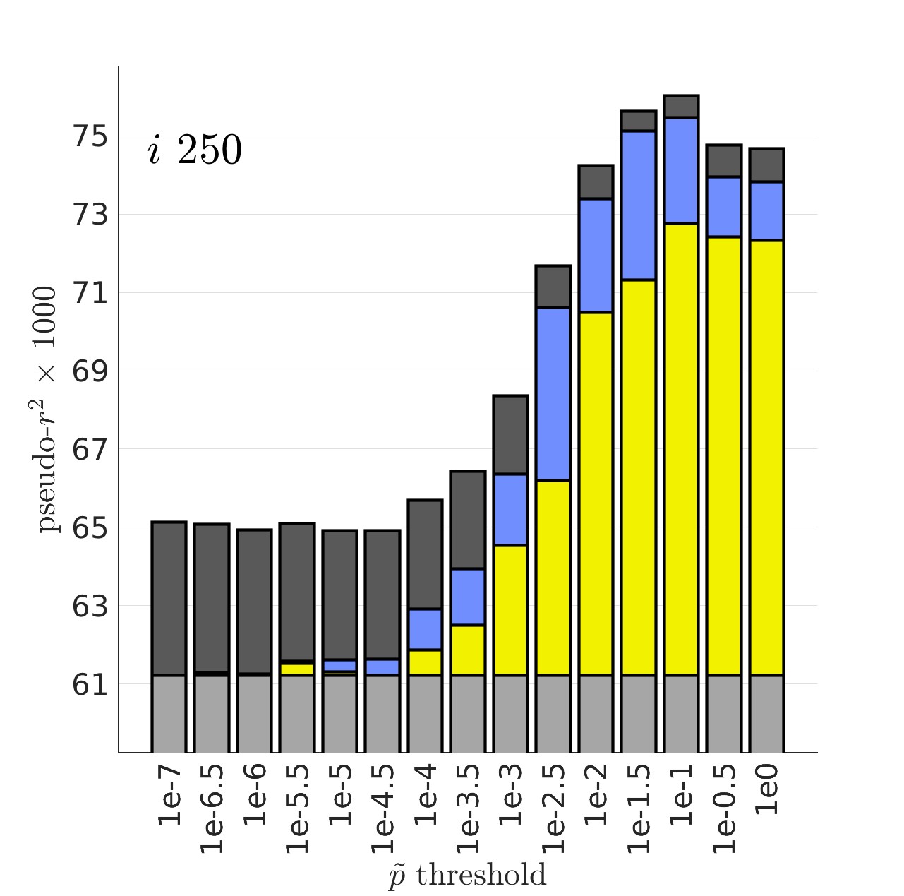
Fig 19: In this figure we illustrate the explanatory power of the bicluster-informed ${\bf PRS_{\text{\footnotesize bicl}}}(j^{\prime};i,\tilde{p})$ in combination with the bicluster-score $u^{\prime}_{j^{\prime}}(i)$ for arm-2, with the iteration number $i$ varying across the subplots. Within each subplot the $\tilde{p}$-threshold is shown along the horizontal-axis. We measure the incremental Nagelkerke pseudo-$r^{2}$ value associated with the following terms: (i) the ancestry-related covariates, (ii) the population-wide ${\bf PRS_{\text{\footnotesize wide}}}(j^{\prime};\tilde{p})$, (iii) the bicluster-informed ${\bf PRS_{\text{\footnotesize bicl}}}(j^{\prime};i,\tilde{p})$, and (iv) the bicluster-score $u^{\prime}_{j^{\prime}}(i)$. For each $i$ and $\tilde{p}$ we show a vertical bar divided into segments illustrating the contribution of each term (i)-(iv), with colors light-grey, yellow, blue-pink and dark-grey (respectively). The colors used for the third term (ranging from blue to pink) correspond to the colors used in Fig 7 below.

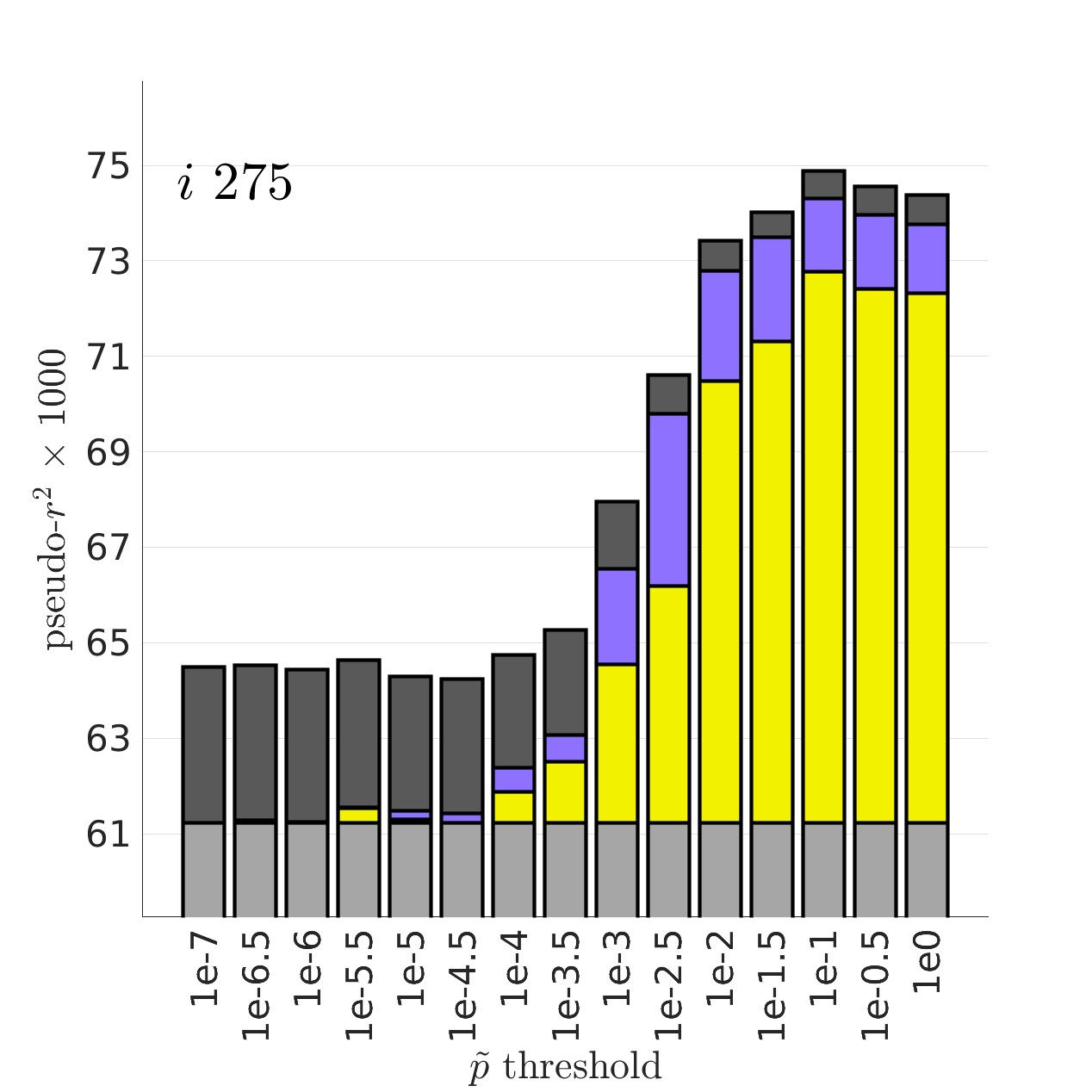
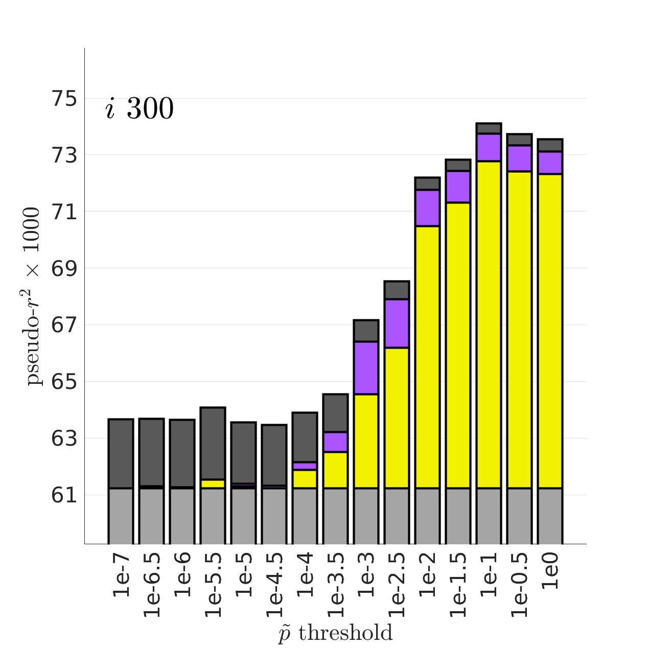
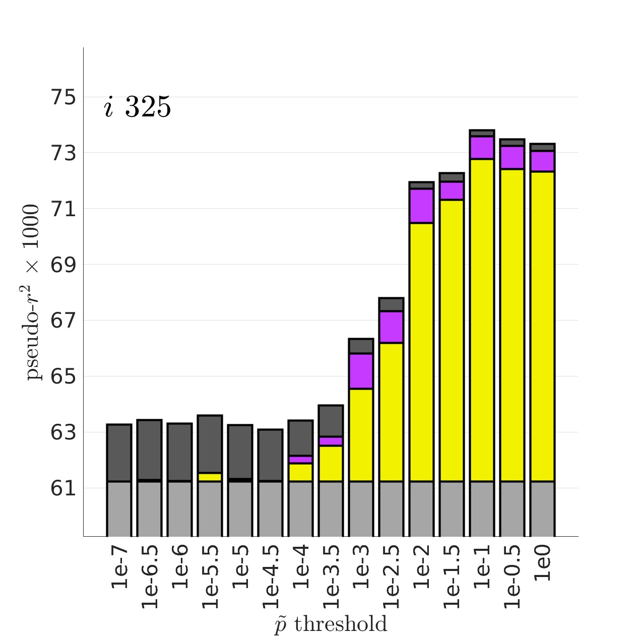
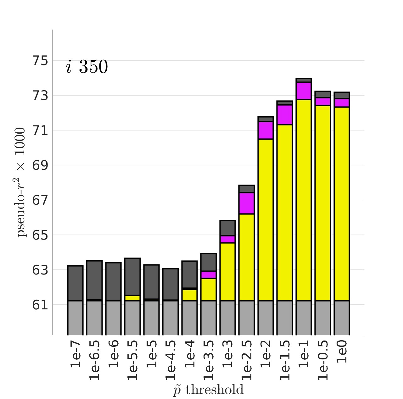
Fig 20: This is analogous to Fig 19, for a different set of iterations.

Replication results for arm-3 and arm-4

Figs 21 and 22 illustrate the replication analyses on arms 3 and 4.

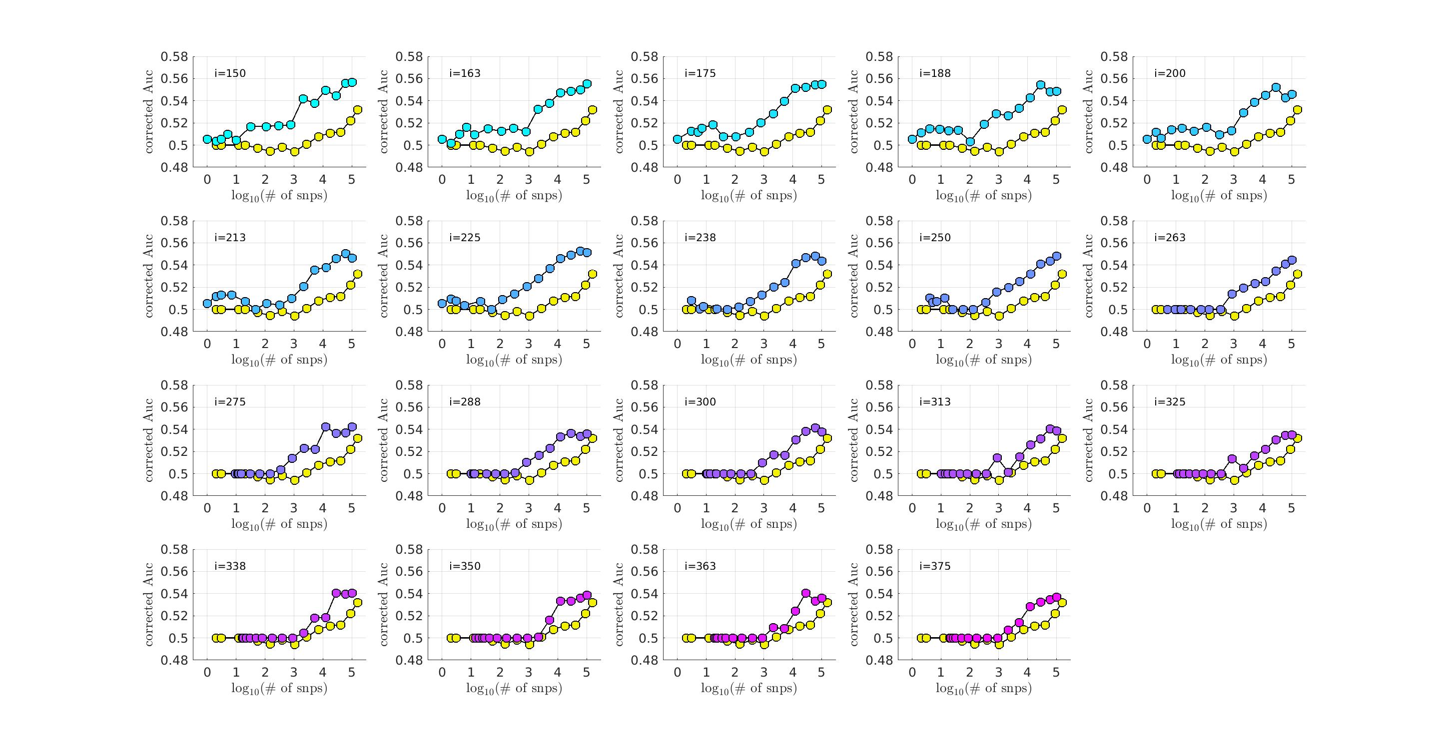
Fig 21: This figure is analogous to Fig 7, except that we test on arm-3 rather than arm-2.

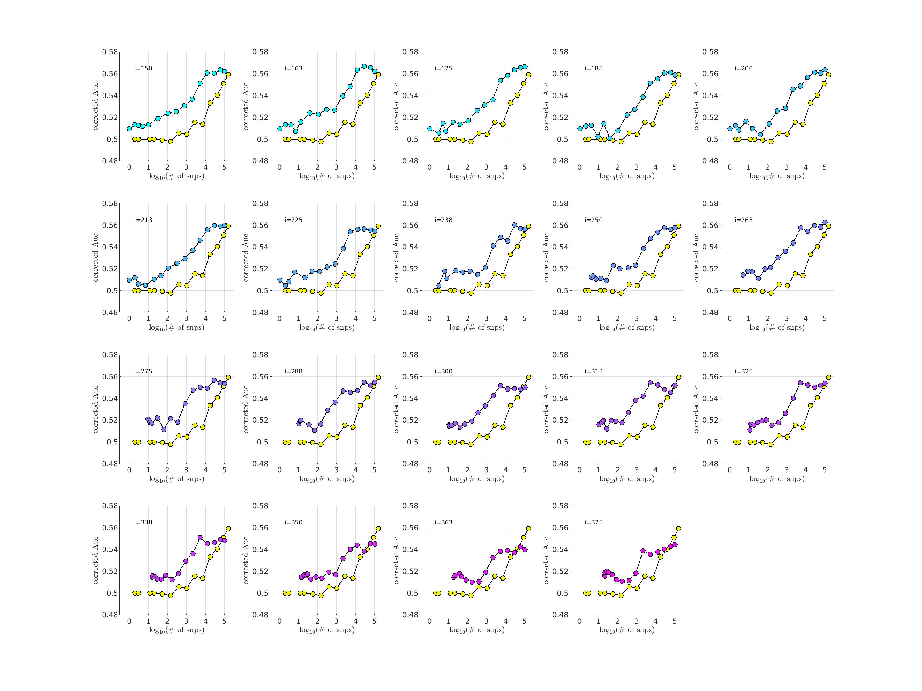
Fig 22: This figure is analogous to Fig 7, except that we test on arm-4 rather than arm-2.

Significance of secondary bicluster in arm-1

Figs 23 24 25 and 26 illustrate the significance of the secondary bicluster found in arm-1.

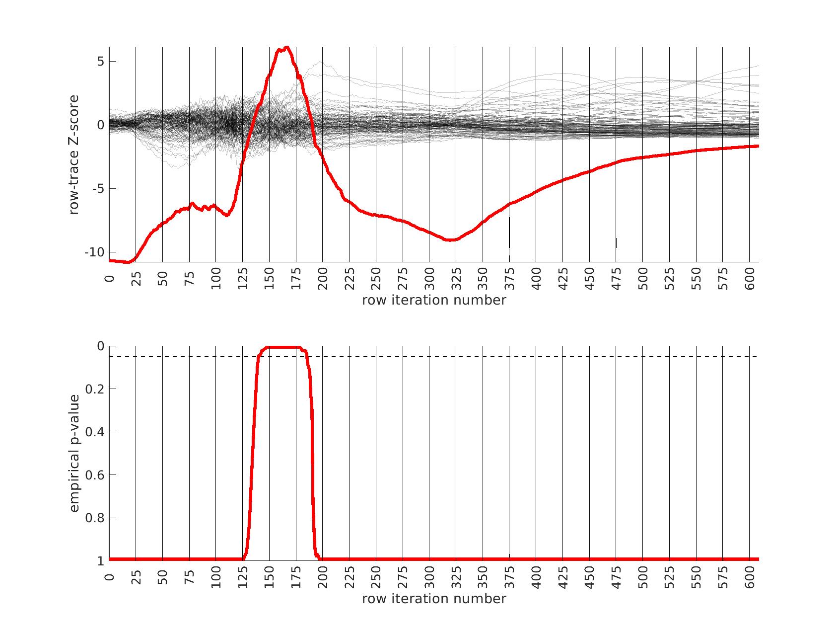
Fig 23: This figure is analogous to Fig 2, except that the red trace corresponds to a search for a secondary bicluster. Note that the red trace is only somewhat significant over a small range of iterations, including $i\in\left[150,175\right]$.

Fig 24: In this figure we illustrate the replication of the secondary bicluster in arm-2. The overall replication p-value is $p=0.86$ (i.e., not significant).

Fig 25: In this figure we illustrate the replication of the secondary bicluster in arm-3. The overall replication p-value is $p=0.41$ (i.e., not significant).

Fig 26: In this figure we illustrate the replication of the secondary bicluster in arm-4. The overall replication p-value is $p=0.85$ (i.e., not significant).

Control-biclusters

Figs 27, 28, 29 and 30 illustrate the replication analyses for the control-biclusters found in arms 2, 3 and 4.

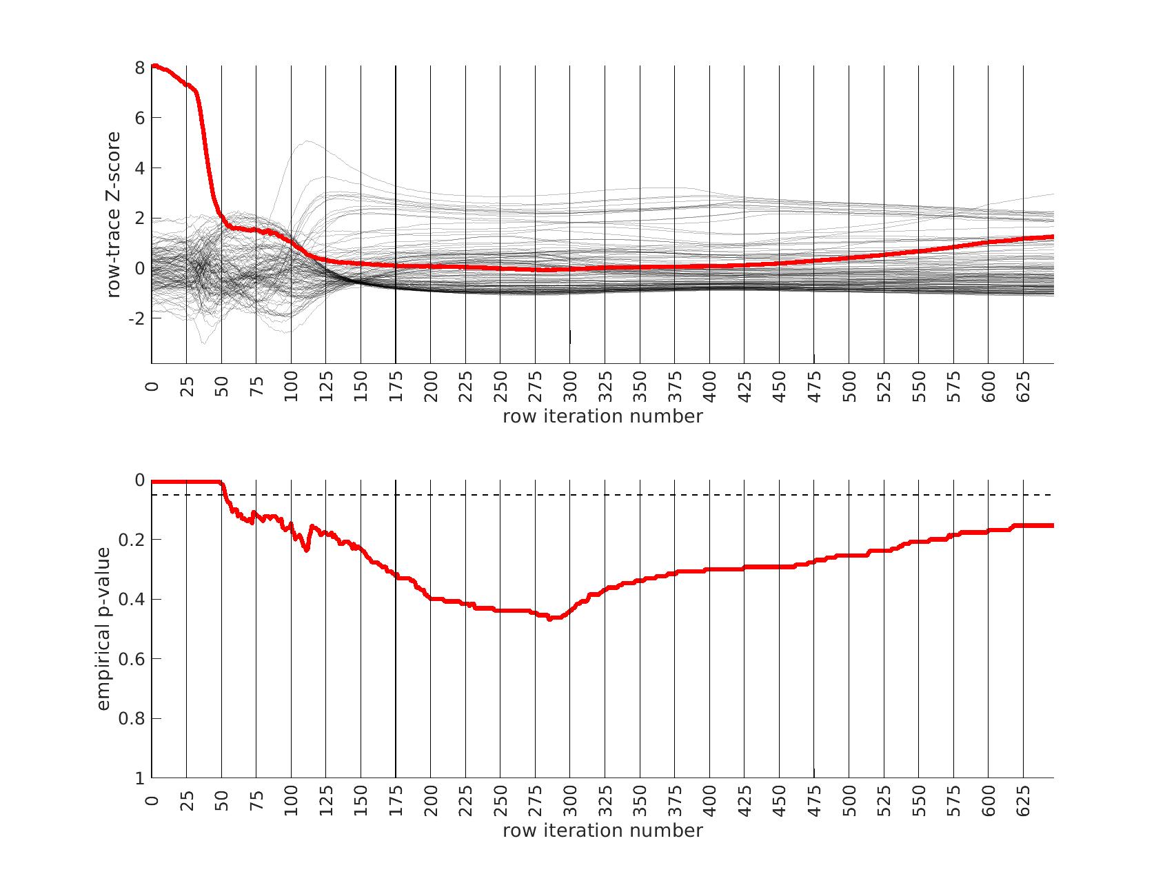
Fig 27: This figure is analogous to Fig 2, except that the red trace corresponds to a search for a bicluster within the control-population of arm-1, rather than the case-population. Note that the red trace decays monotonically, with no distinguished peaks as the algorithm proceeds.

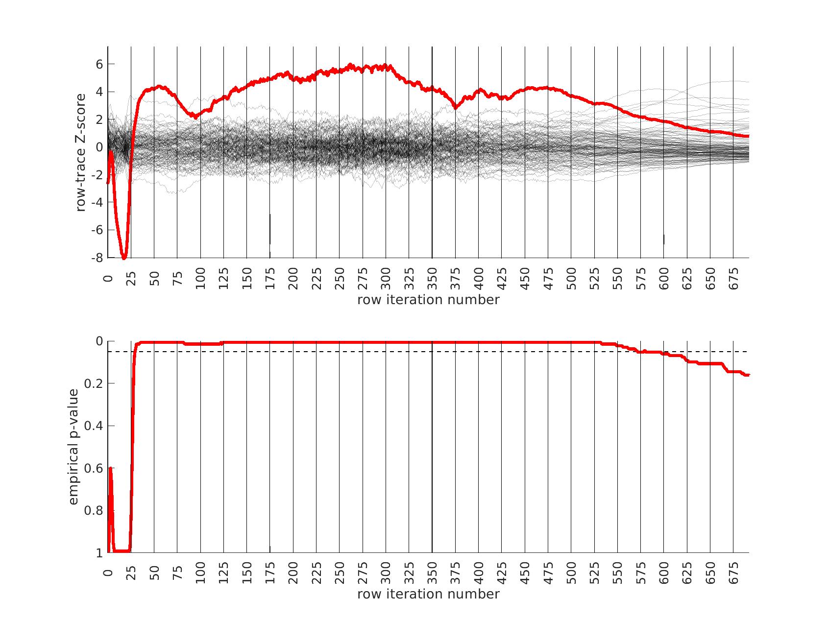
Fig 28: This figure is analogous to Fig 27, except that we consider arm-2 as a training-arm (rather than arm-1). Note that there are multiple distinguished peaks to the red trace, indicating (at least) one bicluster. The overall replication p-value of the dominant bicluster indicated by this trace is $p=0.030$ in arm-3, $p=0.17$ in arm-4 and $p=0.00015$ in arm-1.

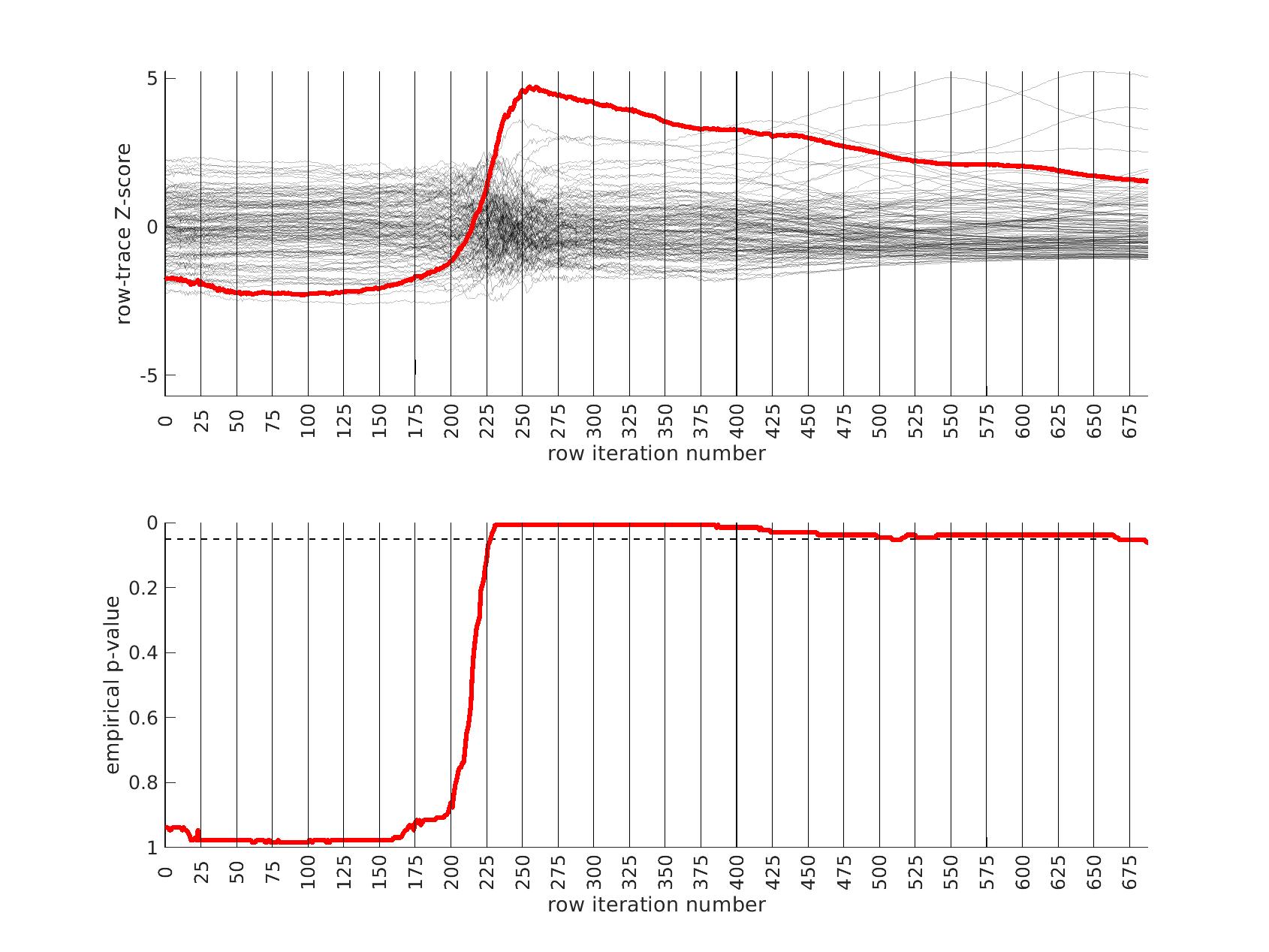
Fig 29: This figure is analogous to Fig 27, except that we consider arm-3 as a training-arm (rather than arm-1). Note that there is a distinguished peak to the red trace, indicating one bicluster. The overall replication p-value of this dominant bicluster is $p=0.00010$ in arm-2, $p=0.0025$ in arm-4, and $p=0.0063$ in arm-1.

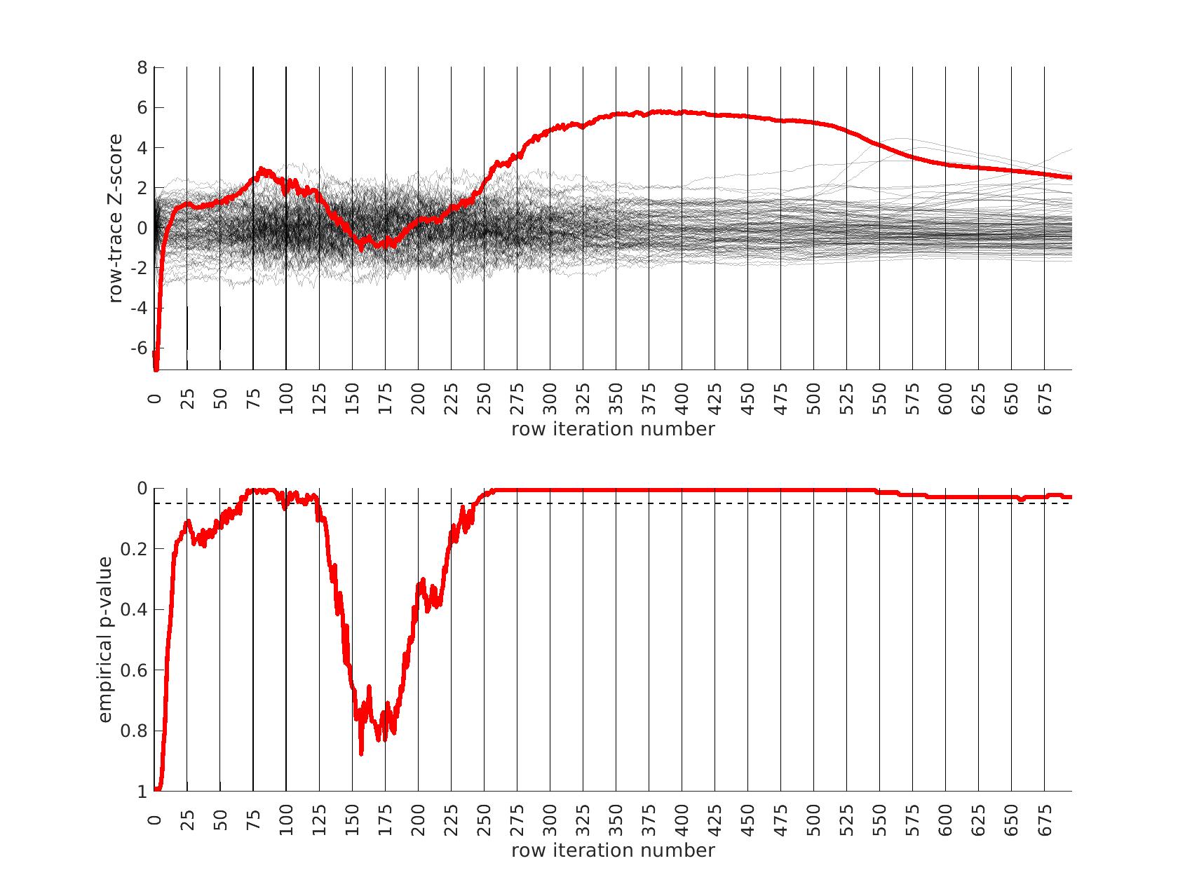
Fig 30: This figure is analogous to Fig 27, except that we consider arm-4 as a training-arm (rather than arm-1). Note that there are multiple distinguished peaks to the red trace, indicating (at least) one bicluster. The overall replication p-value of the dominant bicluster indicated by this trace is $p=0.000025$ in arm-2, $p=0.00013$ in arm-3, and $p=0.040$ in arm-1.

References

- 1. American Psychiatric Association. Diagnostic and statistical manual of mental disorders [5th edition]. Washington, DC 20024:USA: American Psychiatric Association Publishing, 2013.
- 2. J. Angst. The emerging epidemiology of hypomania and bipolar ii disorder. Journal of Affective Disorders, 50:143–151, 1998.
- 3. K. R. Merikangas, H. S. Akiskal, J. Angst, P. E. Greenberg, R. M. A. Hirschfeld, M. Petukhova, and R. C. Kessler. Lifetime and 12-month prevalence of bipolar spectrum disorder in the national comorbidity survey replication. Archives of General Psychiatry, 64:543–552, 2007.
- 4. K. R. Merikangas, R. Jin, J.-P. He, R. C. Kessler, S. Lee, N. A. Sampson, M. C. Viana, …, and Z. Zarkov. Prevalence and correlates of bipolar spectrum disorder in the world mental health survey initiative. Archives of General Psychiatry, 68:241–251, 2011.
- 5. GBD 2016 Disease, Injury Incidence, and Prevalence Collaborators. Global, regional, and national incidence, prevalence, and years lived with disability for 328 diseases and injuries for 195 countries, 1990-2016: A systematic analysis for the global burden of disease study 2016. The Lancet, 390:1211–1259, 2017.
- 6. O. J. Bienvenu, D. S. Davydow, and K. S. Kendler. Psychiatric ‘diseases’ versus behavioral disorders and degree of genetic influence. Psychological Medicine, 41:33–40, 2011.
- 7. N. Craddock and P. Sklar. Genetics of bipolar disorder. The Lancet, 381:1654–1662, 2013.
- 8. K. Merikangas and K. Yu. Genetic epidemiology of bipolar disorder. Clinical Neuroscience Research, 2:127–141, 2002.
- 9. J. W. Smoller and C. T. Finn. Family, twin, and adoption studies of bipolar disorder. American Journal of Medical Genetics. Part C, 2003.
- 10. J. Song, S. E. Bergen, R. Kuja-Halkola, H. Larsson, M. Landén, and P. Lichtenstein. Bipolar disorder and its relation to major psychiatric disorders: A family-based study in the swedish population. Bipolar Disorders, 17:184–193, 2015.
- 11. K. S. Kendler, H. Ohlsson, J. Sundquist, and K. Sundquist. An extended swedish national adoption study of bipolar disorder illness and cross-generational familial association with schizophrenia and major depression. JAMA Psychiatry, 77:814–822, 2020.
- 12. WHO Staff World Health Organization. The icd-10 classification of mental and behavioural disorders: Clinical descriptions and diagnostic guidelines. Geneva, 1992.
- 13. I. Grande, M. Berk, B. Birmaher, and E. Vieta. Bipolar disorder. The Lancet, 387:1561–1572, 2016.
- 14. A. W. Charney, D. M. Ruderfer, E. A. Stahl, J. L. Moran, K. Chambert, R. A. Belliveau, …, and P. Sklar. Evidence for genetic heterogeneity between clinical subtypes of bipolar disorder. Translational Psychiatry, 7:e993, 2017.
- 15. J. Allardyce, G. Leonenko, M. Hamshere, A. F. Pardiñas, L. Forty, S. Knott, …, and V. Escott-Price. Association between schizophrenia-related polygenic liability and the occurrence and level of mood-incongruent psychotic symptoms in bipolar disorder. JAMA Psychiatry, 75:28–35, 2018.
- 16. M. Markota, B. J. Coombes, B. R. Larrabee, S. L. McElroy, D. J. Bond, M. Veldic, …, and J. M. Biernacka. Association of schizophrenia polygenic risk score with manic and depressive psychosis in bipolar disorder. Translational Psychiatry, 8:188, 2018.
- 17. Bipolar Disorder and Schizophrenia Working Group of the Psychiatric Genomics Consortium. Genomic dissection of bipolar disorder and schizophrenia, including 28 subphenotypes. Cell, 173:1705–1715, 2018.
- 18. K. J. S. Lewis, A. Richards, R. Karlsson, G. Leonenko, S. E. Jones, H. J. Jones, …, and A. Di Florio. Comparison of genetic liability for sleep traits among individuals with bipolar disorder i or ii and control participants. JAMA Psychiatry, 77:303–310, 2019.
- 19. A. W. Charney, E. A. Stahl, E. K. Green, C.-Y. Chen, J. L. Moran, K. Chambert, …, and P. Sklar. Contribution of rare copy number variants to bipolar disorder risk is limited to schizoaffective cases. Biological Psychiatry, 86:110–119, 2019.
- 20. E. A. Stahl, G. Breen, A. J. Forstner, A. McQuillin, S. Ripke, …, and V. Trubetskoy. Genome-wide association study identifies 30 loci associated with bipolar disorder. Nature Genetics, 51:793–803, 2019.
- 21. B. Coombes, M. Markota, J. Mann, C. Colby, E. Stahl, A. Talati, …, and J. M. Biernacka. Dissecting clinical heterogeneity of bipolar disorder using multiple polygenic risk scores. medRxiv, 2020.
- 22. A. F. Carvalho, J. Firth, and E. Vieta. Bipolar disorder. The New England Journal of Medicine, 383:58–66, 2020.
- 23. K.S. O’Connel and B.J. Coombes. Genetic contributions to bipolar disorder: current status and future directions. Psychologial Medicine, 51(13):2156–2167, 2021.
- 24. Amare International Consortium on Lithium Genetics [ConLi + Gen], Schubert A. T., Hou K. O., Clark L., Papiol S. R., …, and S. … Baune. Association of polygenic score for schizophrenia and hla antigen and inflammation genes with response to lithium in bipolar affective disorder: A genome-wide association study. JAMA Psychiatry, 75:65–74, 2018.
- 25. A. T. Amare, K. O. Schubert, L. Hou, S. R. Clark, S. Papiol, M. Cearns, …, and B. T. Baune. Association of polygenic score for major depression with response to lithium in patients with bipolar disorder. Nature, Molecular Psychiatry, 26:2457–2470, 2021.
- 26. A. Nunes, T. Trappenberg, and M. Alda. Asymmetrical reliability of the alda score favours a dichotomous representation of lithium responsiveness. PLoS ONE, 15:e0225353, 2020.
- 27. F. J. A. Gordovez and F. J. McMahon. The genetics of bipolar disorder. Molecular Psychiatry, 25:544–559, 2020.
- 28. A. M.-C. Ho, B. J. Coombes, T. T. L. Nguyen, D. Liu, S. L. McElroy, B. Singh, …, and J. M. Biernacka. Mood-stabilizing antiepileptic treatment response in bipolar disorder: A genome-wide association study. Clinical Pharmacology and Therapeutics, 108:1233–1242, 2020.
- 29. N. Mullins, A. J. Forstner, K. S. O’Connell, B. Coombes, J. R. I. Coleman, Z. Qiao, …, and O. A. Andreassen. Genome-wide association study of over 40000 bipolar disorder cases provides novel biological insights. medRxiv, 2020.
- 30. M. Gatz, C. A. Reynolds, L. Fratiglioni, B. Johansson, J. A. Mortimer, S. Berg, …, and N. L. Pedersen. Role of genes and environments for explaining alzheimer disease. Archives of General Psychiatry, 63:168–174, 2006.
- 31. H. A. Browne, S. L. Gair, J. M. Scharf, and D. E. Grice. Genetics of obsessive-compulsive disorder and related disorders. The Psychiatric Clinics of North America, 37:319–335, 2014.
- 32. N. R. Zilhão, M. C. Olthof, D. J. A. Smit, D. C. Cath, L. Ligthart, C. A. Mathews, …, and C. V. Dolan. Heritability of tic disorders: A twin-family study. Psychological Medicine, 47:1085–1096, 2017.
- 33. R. K. Walters, R. Polimanti, E. C. Johnson, J. N. McClintick, M. J. Adams, A. E. Adkins, …, and A. Agrawal. Transancestral gwas of alcohol dependence reveals common genetic underpinnings with psychiatric disorders. Nature Neuroscience, 21:1656–1669, 2018.
- 34. Cross-Disorder Group of the Psychiatric Genomics Consortium. Genomic relationships, novel loci, and pleiotropic mechanisms across eight psychiatric disorders. Cell, 179:1469–1482, 2019.
- 35. D. Demontis, V. M. Rajagopal, T. E. Thorgeirsson, T. D. Als, J. Grove, K. Leppälä, …, and A. D. Børglum. Genome-wide association study implicates chrna2 in cannabis use disorder. Nature Neuroscience, 22:1066–1074, 2019.
- 36. S. V. Faraone and H. Larsson. Genetics of attention deficit hyperactivity disorder. Molecular Psychiatry, 24:562–575, 2019.
- 37. I. E. Jansen, J. E. Savage, K. Watanabe, J. Bryois, D. M. Williams, S. Steinberg, …, and D. Posthuma. Genome-wide meta-analysis identifies new loci and functional pathways influencing alzheimer’s disease risk. Nature Genetics, 51:404–413, 2019.
- 38. K. L. Purves, J. R. I. Coleman, S. M. Meier, C. Rayner, K. A. S. Davis, R. Cheesman, …, and T. C. Eley. A major role for common genetic variation in anxiety disorders. Molecular Psychiatry, 25:3292–3303, 2020.
- 39. S. Djurovic, O. Gustafsson, M. Mattingsdal, L. Athanasiu, T. Bjella, M. Tesli, …, and O. A. Andreassen. A genome-wide association study of bipolar disorder in norwegian individuals, followed by replication in icelandic sample. Journal of Affective Disorders, 126:312–316, 2010.
- 40. E. N. Smith, D. L. Koller, C. Panganiban, S. Szelinger, P. Zhang, J. A. Badner, …, and J. R. Kelsoe. Genome-wide association of bipolar disorder suggests an enrichment of replicable associations in regions near genes. PLoS Genetics, 7:e1002134, 2011.
- 41. S. J. Winham, A. B. Cuellar-Barboza, A. Oliveros, S. L. McElroy, S. Crow, C. Colby, …, and J. M. Biernacka. Genome-wide association study of bipolar disorder accounting for effect of body mass index identifies a new risk allele in tcf7l2. Molecular Psychiatry, 19:1010–1016, 2014.
- 42. M. Aas, U. K. Haukvik, S. Djurovic, M. Tesli, L. Athanasiu, T. Bjella, …, and I. Melle. Interplay between childhood trauma and bdnf val66met variants on blood bdnf mrna levels and on hippocampus subfields volumes in schizophrenia spectrum and bipolar disorders. Journal of Psychiatric Research, 59:14–21, 2014.
- 43. J. Oliveira, R. Kazma, E. Le Floch, M. Bennabi, N. Hamdani, D. Bengoufa, …, and R. Tamouza. Toxoplasma gondii exposure may modulate the influence of tlr2 genetic variation on bipolar disorder: A gene–environment interaction study. International Journal of Bipolar Disorders, 2016.
- 44. G. M. Hosang, H. L. Fisher, S. Cohen-Woods, P. McGuffin, and A. E. Farmer. Stressful life events and catechol-o-methyl-transferase (comt) gene in bipolar disorder. Depression and Anxiety, 34:419–426, 2017.
- 45. M. Aas, F. Bellivier, F. Bettella, C. Henry, S. Gard, J.-P. Kahn, …, and B. Etain. Childhood maltreatment and polygenic risk in bipolar disorders. Bipolar Disorders, 22:174–181, 2020.
- 46. Purcell International Schizophrenia Consortium, Wray S. M., Stone N. R., Visscher J. L., O’Donovan P. M., …, and M. C. … Sklar. Common polygenic variation contributes to risk of schizophrenia and bipolar disorder. Nature, 460:748–752, 2009.
- 47. H. C. Wilcox, J. M. Fullerton, A. L. Glowinski, K. Benke, M. Kamali, L. A. Hulvershorn, …, and J. I. Nurnberger. Traumatic stress interacts with bipolar disorder genetic risk to increase risk for suicide attempts. Journal of the American Academy of Child and Adolescent Psychiatry, 56:1073–1080, 2017.
- 48. S. Mistry, J. R. Harrison, D. J. Smith, V. Escott-Price, and S. Zammit. The use of polygenic risk scores to identify phenotypes associated with genetic risk of bipolar disorder and depression: A systematic review. Journal of Affective Disorders, 234:148–155, 2018.
- 49. G. W. Reginsson, A. Ingason, J. Euesden, G. Bjornsdottir, S. Olafsson, E. Sigurdsson, …, and K. Stefansson. Polygenic risk scores for schizophrenia and bipolar disorder associate with addiction. Addiction Biology, 23:485–492, 2018.
- 50. S. Mistry, V. Escott-Price, A. D. Florio, D. J. Smith, and S. Zammit. Genetic risk for bipolar disorder and psychopathology from childhood to early adulthood. Journal of Affective Disorders, 246:633–639, 2019.
- 51. S. Mistry, V. Escott-Price, A. D. Florio, D. J. Smith, and S. Zammit. Investigating associations between genetic risk for bipolar disorder and cognitive functioning in childhood. Journal of Affective Disorders, 259:112–120, 2019.
- 52. K. L. Musliner, P. B. Mortensen, J. J. McGrath, N. P. Suppli, D. M. Hougaard, …, and J. Bybjerg-Grauholm. Association of polygenic liabilities for major depression, bipolar disorder, and schizophrenia with risk for depression in the danish population. JAMA Psychiatry, 76:516–525, 2019.
- 53. K. L. Musliner, M. D. Krebs, C. Albiñana, B. Vilhjalmsson, E. Agerbo, P. P. Zandi, …, and S. D. Østergaard. Polygenic risk and progression to bipolar or psychotic disorders among individuals diagnosed with unipolar depression in early life. American Journal of Psychiatry, 177:936–943, 2020.
- 54. N. Mullins, T. B. Bigdeli, A. D. Børglum, J. R. I. Coleman, D. Demontis, D. Mehta, …, and C. M. Lewis. Gwas of suicide attempt in psychiatric disorders and association with major depression polygenic risk scores. The American Journal of Psychiatry, 176:651–660, 2019.
- 55. M. Grigoroiu-Serbanescu, G. Giaroli, J. H. Thygesen, O. Shenyan, T. B. Bigdeli, N. J. Bass, …, and A. McQuillin. Predictive power of the adhd gwas 2019 polygenic risk scores in independent samples of bipolar patients with childhood adhd. Journal of Affective Disorders, 265:651–659, 2020.
- 56. D. T. Chen, X. Jiang, N. Akula, Y. Y. Shugart, J. R. Wendland, C. J. M. Steele, …, and J. Strauss. Genome-wide association study meta-analysis of european and asian-ancestry samples identifies three novel loci associated with bipolar disorder. Molecular Psychiatry, 18:195–205, 2013.
- 57. C. Joslyn, D. J. Hawes, C. Hunt, and P. B. Mitchell. Is age of onset associated with severity, prognosis, and clinical features in bipolar disorder? a meta-analytic review. Bipolar Disorders, 18:389–403, 2016.
- 58. H. Y. Eser, A. S. Kacar, C. M. Kilciksiz, M. Yalçinay-Inan, and D. Ongur. Prevalence and associated features of anxiety disorder comorbidity in bipolar disorder: A meta-analysis and meta-regression study. Frontiers in Psychiatry, 9:229, 2018.
- 59. 23andMe. Research consent document. https://www.23andme.com/about/consent/, 2023. [Online; accessed 19-Dec-2023].
- 60. C. McGrouther. Confounding factors in association studies of neuropsychiatric disease: A case study of Bipolar Affective Disorder. Ph.d. thesis, University of California, San Diego, San Diego, CA, 2014.
- 61. Katie J. S. Lewis, Alexander Richards, Robert Karlsson, Ganna Leonenko, Samuel E. Jones, Hannah J. Jones, Katherine Gordon-Smith, Liz Forty, Valentina Escott-Price, Michael J. Owen, Michael N. Weedon, Lisa Jones, Nick Craddock, Ian Jones, Mikael Landén, Michael C. O’Donovan, and Arianna Di Florio. Comparison of Genetic Liability for Sleep Traits Among Individuals With Bipolar Disorder I or II and Control Participants. JAMA Psychiatry, 77(3):303–310, 03 2020.
- 62. J. Xie, A. Ma, A. Fennell, Q. Ma, and J. Zhao. It is time to apply biclustering: a comprehensive review of biclustering applications in biological and biomedical data. Brief Bioinform, 20(4):1449–1464, 2019.
- 63. A. Dahl and N. Zaitlen. Genetic influences on disease subtypes. Annu Rev Genomics Hum Genet, 21:413–435, 2020.
- 64. Aaditya V. Rangan. A simple filter for detecting low-rank submatrices. Journal of Computational Physics, 231(7):2682–2690, April 2012.
- 65. Aaditya V. Rangan, Caroline C. McGrouther, John Kelsoe, Nicholas Schork, Eli Stahl, Qian Zhu, Arjun Krishnan, Vicky Yao, Olga Troyanskaya, Seda Bilaloglu, Preeti Raghavan, Sarah Bergen, Anders Jureus, Mikael Landen, and Bipolar Disorders Working Group of the Psychiatric Genomics Consortium. A loop-counting method for covariate-corrected low-rank biclustering of gene-expression and genome-wide association study data. PLOS Computational Biology, 14(5):1–29, 05 2018.
- 66. Wellcome Trust Case Control Consortium. Genome-wide association study of 14 000 cases of seven common diseases and 3000 shared controls. Nature, 447:661–678, 2007.
- 67. Lisa Jones, Alice Metcalf, Katherine Gordon-Smith, Liz Forty, Amy Perry, Joanne Lloyd, John R. Geddes, Guy M. Goodwin, Ian Jones, Nick Craddock, and et al. Gambling problems in bipolar disorder in the uk: Prevalence and distribution. British Journal of Psychiatry, 207(4):328–333, 2015.
- 68. Noga Alon, Michael Krivelevich, and Benny Sudakov. Finding a large hidden clique in a random graph. Random Structures & Algorithms, 13(3-4):457–466, 1998.
- 69. Yash Deshpande and Andrea Montanari. Improved sum-of-squares lower bounds for hidden clique and hidden submatrix problems, 2015.
- 70. Shane et al. McCarthy. A reference panel of 64,976 haplotypes for genotype imputation. Nature genetics, 48(10):1279–83, 2016.
- 71. Q. Zhu, A.K. Wong, A. Krishnan, M.R. Aure, A. Tadych, R. Zhang, D.C. Corney, C.S. Greene, L.A. Bongo, V.N. Kristensen, M. Charikar, K. Li, and O.G. Troyanskaya. Targeted exploration and analysis of large cross-platform human transcriptomic compendia. Nature Methods, 12(3):211–214, 2015.
- 72. H. R. Kranzler, H. Zhou, R. L. Kember, R. Vickers Smith, A. C. Justice, S. Damrauer, …, and J. Gelernter. Genome-wide association study of alcohol consumption and use disorder in 274 424 individuals from multiple populations. Nature Communications, 10:1499, 2019.
- 73. S.-K. Jang, G. Saunders, M. Liu, Y. Jiang, D. J. Liu, and S. Vrieze. Genetic correlation, pleiotropy, and causal associations between substance use and psychiatric disorder. Psychological Medicine, 2020.
- 74. K. J. E. van Hulzen, C. J. Scholz, B. Franke, S. Ripke, M. Klein, A. McQuillin, …, and A. Reif. Genetic overlap between attention-deficit/hyperactivity disorder and bipolar disorder: Evidence from genome-wide association study meta-analysis. Biological Psychiatry, 82:634–641, 2017.
- 75. K. S. O’Connell, N. W. McGregor, C. Lochner, R. Emsley, and L. Warnich. The genetic architecture of schizophrenia, bipolar disorder, obsessive-compulsive disorder and autism spectrum disorder. Molecular and Cellular Neurosciences, 88:300–307, 2018.
- 76. J. R. I. Coleman, H. A. Gaspar, J. Bryois, Major Depressive Disorder Working Group of the Psychiatric Genomics Consortium Bipolar Disorder Working Group of the Psychiatric Genomics Consortium, and G. Breen. The genetics of the mood disorder spectrum: Genome-wide association analyses of more than 185 000 cases and 439 000 controls. Biological Psychiatry, 88:169–184, 2020.
- 77. Á. Frías, I. Baltasar, and B. Birmaher. Comorbidity between bipolar disorder and borderline personality disorder: Prevalence, explanatory theories, and clinical impact. Journal of Affective Disorders, 202:210–219, 2016.
- 78. I. M. Salloum and E. S. Brown. Management of comorbid bipolar disorder and substance use disorders. The American Journal of Drug and Alcohol Abuse, 43:366–376, 2017.
- 79. B. Bortolato, M. Berk, M. Maes, R. S. McIntyre, and A. F. Carvalho. Fibromyalgia and bipolar disorder: Emerging epidemiological associations and shared pathophysiology. Current Molecular Medicine, 16:119–136, 2016.
- 80. C. U. Correll, M. Solmi, N. Veronese, B. Bortolato, S. Rosson, P. Santonastaso, …, and B. Stubbs. Prevalence, incidence and mortality from cardiovascular disease in patients with pooled and specific severe mental illness: A large-scale meta-analysis of 3 211 768 patients and 113 383 368 controls. World Psychiatry: Official Journal of the World Psychiatric Association, 16:163–180, 2017.
- 81. D. Vancampfort, C. U. Correll, B. Galling, M. Probst, M. De Hert, P. B. Ward, …, and B. Stubbs. Diabetes mellitus in people with schizophrenia, bipolar disorder and major depressive disorder: A systematic review and large scale meta-analysis. World Psychiatry: Official Journal of the World Psychiatric Association, 15:166–174, 2016.
- 82. B. Roshanaei-Moghaddam and W. Katon. Premature mortality from general medical illnesses among persons with bipolar disorder: A review. Psychiatric Services, 60:147–156, 2009.
- 83. L. V. Kessing, E. Vradi, R. S. McIntyre, and P. K. Andersen. Causes of decreased life expectancy over the life span in bipolar disorder. Journal of Affective Disorders, 180:142–147, 2015.
- 84. A. Diflorio and I. Jones. Is sex important? gender differences in bipolar disorder. International Review of Psychiatry, 22:437–452, 2010.
- 85. A. M. A. Nivoli, I. Pacchiarotti, A. R. Rosa, D. Popovic, A. Murru, M. Valenti, …, and F. Colom. Gender differences in a cohort study of 604 bipolar patients: The role of predominant polarity. Journal of Affective Disorders, 133:443–449, 2011.
- 86. M. Zimmerman, C. J. Ruggero, I. Chelminski, and D. Young. Is bipolar disorder overdiagnosed? The Journal of Clinical Psychiatry, 69:935–940, 2008.
- 87. F. S. Goes, M. Pirooznia, J. S. Parla, M. Kramer, E. Ghiban, S. Mavruk, …, and J. B. Potash. Exome sequencing of familial bipolar disorder. JAMA Psychiatry, 73:590–597, 2016.
- 88. A. Maaser, A. J. Forstner, J. Strohmaier, J. Hecker, K. U. Ludwig, …, and S. Sivalingam. Exome sequencing in large, multiplex bipolar disorder families from cuba. PLoS ONE, 13:e0205895, 2018.
- 89. C. Toma, A. D. Shaw, R. J. N. Allcock, A. Heath, K. D. Pierce, P. B. Mitchell, …, and J. M. Fullerton. An examination of multiple classes of rare variants in extended families with bipolar disorder. Translational Psychiatry, 8:65, 2018.
- 90. F. S. Goes, M. Pirooznia, M. Tehan, P. P. Zandi, J. McGrath, P. Wolyniec, …, and A. E. Pulver. De novo variation in bipolar disorder. Molecular Psychiatry, 387:1561, 2019.
- 91. A. J. Forstner, S. B. Fischer, L. M. Schenk, J. Strohmaier, A. Maaser-Hecker, C. S. Reinbold, …, and S. Cichon. Whole-exome sequencing of 81 individuals from 27 multiply affected bipolar disorder families. Translational Psychiatry, 10:57, 2020.
- 92. J. H. Sul, S. K. Service, A. Y. Huang, V. Ramensky, S.-G. Hwang, T. M. Teshiba, …, and N. B. Freimer. Contribution of common and rare variants to bipolar disorder susceptibility in extended pedigrees from population isolates. Translational Psychiatry, 10:74, 2020.
- 93. M. O. Akinhanmi, J. M. Biernacka, S. M. Strakowski, S. L. McElroy, J. E. Balls Berry, K. R. Merikangas, …, and M. A. Frye. Racial disparities in bipolar disorder treatment and research: A call to action. Bipolar Disorders, 20:506–514, 2018.
- 94. A. R. Martin, M. Kanai, Y. Kamatani, Y. Okada, B. M. Neale, and M. J. Daly. Clinical use of current polygenic risk scores may exacerbate health disparities. Nature Genetics, 51:584–591, 2019.
- 95. R. E. Peterson, K. Kuchenbaecker, R. K. Walters, C.-Y. Chen, A. B. Popejoy, S. Periyasamy, …, and L. E. Duncan. Genome-wide association studies in ancestrally diverse populations: Opportunities, methods, pitfalls, and recommendations. Cell, 179:589–603, 2019.
- 96. G. Sirugo, S. M. Williams, and S. A. Tishkoff. The missing diversity in human genetic studies. Cell, 177:1080, 2019.
- 97. L. Duncan, H. Shen, B. Gelaye, J. Meijsen, K. Ressler, M. Feldman, …, and B. Domingue. Analysis of polygenic risk score usage and performance in diverse human populations. Nature Communications 10(1), 2019.