Information-Theoretic Opacity-Enforcement in Markov Decision Processes

Abstract

The paper studies information-theoretic opacity, an information-flow privacy property, in a setting involving two agents: A planning agent who controls a stochastic system and an observer who partially observes the system states. The goal of the observer is to infer some secret, represented by a random variable, from its partial observations, while the goal of the planning agent is to make the secret maximally opaque to the observer while achieving a satisfactory total return. Modeling the stochastic system using a Markov decision process, two classes of opacity properties are considered—Last-state opacity is to ensure that the observer is uncertain if the last state is in a specific set and initial-state opacity is to ensure that the observer is unsure of the realization of the initial state. As the measure of opacity, we employ the Shannon conditional entropy capturing the information about the secret revealed by the observable. Then, we develop primal-dual policy gradient methods for opacity-enforcement planning subject to constraints on total returns. We propose novel algorithms to compute the policy gradient of entropy for each observation, leveraging message passing within the hidden Markov models. This gradient computation enables us to have stable and fast convergence. We demonstrate our solution of opacity-enforcement control through a grid world example.

1 Introduction

Opacity, as a plural concept, has been proposed to generalize secrecy, anonymity, privacy, and other confidentiality properties against attacks Zeng and Koutny (2021); Watson (2011); Guo et al. (2020). Opacity enforcement is to hide sensitive information from an external observer.

Depending on the various measures of opacity, two classes of opacity enforcement problems have been investigated: Qualitative opacity enforcement requires that an adversary/observer, with complete knowledge of the system yet noisy observations, can ascertain some “secret” information of the system with probability one. Quantitative opacity enforcement, on the other hand, requires that the observer’s uncertainty in guessing the secret after receiving the observations is close to the uncertainty the observer initially had. Connecting with the classical work of Shannon on secrecy Shannon (1949) and guesswork Khouzani and Malacaria (2017), we propose to measure quantitative opacity using the conditional entropy of the random variable (e.g. the observer’s estimate of a secret variable $Z$) given the observed information (e.g. the observation sequence $Y$). This is because: $\text{The leaked information}=$

$$\underbrace{\text{initial uncertainty}}_{H(Z)-\text{``entropy before observation''}}-\underbrace{\text{remaining uncertainty}}_{H(Z|Y)-\text{`` entropy after observation''}}$$

The more opaque the system is, the larger the entropy after the observation. With this notion of quantitative opacity, we study optimal opacity-enforcement planning in a stochastic system modeled as a Markov decision process (MDP) subject to task performance constraints. We consider the interaction between a planning agent (referred to as player 1/P1) and an observer (referred to as player 2/P2). The goal of P1 is to maximize the opacity while ensuring that the total return meets a satisfying threshold, against P2 who has partial observations about the system trajectories but complete knowledge about the system model and P1’s control policy. Two problems of state-based opacity are studied. One is the last-state opacity, where P1 aims to obfuscate if the last state is in a set of secret states, to P2. The other one is initial-state opacity, where P1 aims to obfuscate the exact initial state to P2.

Related work Opacity was originally introduced by Mazaré (2004), referring to concealing secrets from an observer. This work has led to various qualitative analyses of opacity within discrete event systems (DESs), where the system dynamics are governed by both controllable and uncontrollable events, and its information leakage is also defined by observable and non-observable events. In qualitative analysis, a trajectory is opaque if it satisfies some secret property and is indistinguishable from at least one trajectory that does not satisfy the secret. A system is opaque if it generates only an opaque trajectory.

Different types of qualitative opacity have been studied, including state-based, which requires the secret behavior of the system (i.e., the membership of its initial/current/past state to the set) to remain opaque Saboori and Hadjicostis (2007, 2013a); Han et al. (2023); Saboori and Hadjicostis (2013b, 2009); Yin et al. (2019); language-based Dubreil et al. (2008); Lin (2011); Shi et al. (2023), which aims to hide a set of secret executions; and “model-based” Keroglou and Hadjicostis (2016), aiming to prevent the observer from finding out the true model of the system among several candidates.

While qualitative opacity evaluates whether a system is opaque, a quantitative analysis of opacity is essential for measuring the degree of opacity in a system. Bérard et al. (2015a) defines quantitative opacity as the probability of generating an opaque run in a stochastic system. A related notion to quantitative opacity is covertness Marzouqi and Jarvis (2004, 2005), which measures the distance to the risk of being observed during the planning of a path to a predefined destination. This can be viewed as a model-based opacity, as it makes the observer uncertain if a covert agent is present or not. Recent work Ma et al. (2023) studies how covert planning can leverage the coupling of stochastic dynamics and observational noises to make the covert agent’s policy indistinguishable from a nominal policy.

An alternative approach involves the utilization of the value of information (VOI). Khouzani and Malacaria (2017) employed entropy as a measure of VOI to enforce opacity in channel design problems. The channel design problem can be viewed as a one-step decision-making problem. Recent work adds a linear temporal logic constraint to the entropy maximization problem on MDP Savas et al. (2020). Another recent work Molloy and Nair (2023) developed a method for obfuscating state trajectories in partially observable Markov decision processes (POMDPs) and shows that the conditional entropy of the state trajectory can be expressed into a cumulative sum of entropy terms, permitting the use of POMDP solvers to maximize/minimize the conditional entropy.

Our contribution Our work can be seen as a generalization of minimal information leakage channel design from one-stage decision-making to sequential decision-making in Markov decision processes, concerning state-based opacity. We establish the last-state opacity and initial-state opacity by leveraging Shannon entropy Shannon (1949) as a symmetric measure of opacity. Different from Molloy and Nair (2023), we do not assume that the observer has access to control inputs. Thus, the conditional entropy of state-based opacity properties cannot be constructed as a cumulative sum of entropy terms. We propose a novel approach to compute/estimate the gradient of the conditional entropy with respect to (w.r.t.) the parameters of the control policy, leveraging the forward-backward algorithm in HMMs. Building on the gradient estimation/computation, we can then formulate the optimal opacity enforcement planning problem, subject to task constraints, into a constrained optimization and employ primal-dual gradient-based optimization to compute a (locally)-optimal policy that maximizes the opacity while satisfying a constraint on the total return. The correctness of the proposed methods is experimentally validated.

2 Preliminary and Problem Formulation

2.1 Preliminaries

Notation

The set of real numbers is denoted by $\mathbf{R}$. Random variables will be denoted by capital letters, and their realizations by lowercase letters (e.g., $X$ and $x$). The probability mass function (pmf) of a discrete random variable $X$ will be written as $p(x)$, the joint pmf of $X$ and $Y$ as $p(x,y)$, and the conditional pmf of $X$ given $Y=y$ as $p(x|y)$ or $p(x|Y=y)$. The sequence of random variables and their realizations with length $T$ are denoted as $X_{[0:T]}$ and $x_{[0:T]}$, respectively. Given a finite and discrete set $\mathcal{S}$, let $\mathcal{D}(\mathcal{S})$ be the set of all probability distributions over $\mathcal{S}$. The set $\mathcal{S}^{T}$ denotes the set of sequences with length $T$ composed of elements from $\mathcal{S}$ and $\mathcal{S}^{\ast}$ denotes the set of all finite sequences generated from $\mathcal{S}$.

The Planning Problem

The problem is modeled as a MDP $M=\langle\mathcal{S},\mathcal{A},P,\mu_{0},R,\gamma\rangle$ where $\mathcal{S}$ is a finite set of states, $\mathcal{A}$ is a finite set of actions, $P:\mathcal{S}\times\mathcal{A}\rightarrow\mathcal{D}(\mathcal{S})$ is a probabilistic transition function and $P(s^{\prime}|s,a)$ is the probability of reaching state $s^{\prime}$ given that action $a$ is taken at the state $s$. $\mu_{0}$ is the initial state distribution. The planning objective is described by a reward function $R:\mathcal{S}\times\mathcal{A}\rightarrow\mathbf{R}$. $\gamma\in[0,1]$ is the discount factor.

We refer to the planning agent as player 1, or P1, and the observer as player 2, or P2. For a Markov policy $\pi:\mathcal{S}\rightarrow\mathcal{D}(\mathcal{A})$, P1’s value function $V^{\pi}:\mathcal{S}\rightarrow\mathbf{R}$ is defined as

$$V^{\pi}(s)=E_{\pi}[\sum\limits_{k=0}^{\infty}\gamma^{k}R(S_{k},\pi(S_{k}))|S_{0}=s],$$

where $E_{\pi}$ is the expectation w.r.t. the probability distribution induced by the policy $\pi$ from $M$. We denote the Markov chain induced by the policy $\pi$ as $M_{\pi}$. And $S_{k}$ is the $k$-th state in the Markov chain $M_{\pi}$. P2’s observation function is a common knowledge, defined as follows:

Definition 1 (Observation function of P2).

Let $\mathcal{O}$ be a finite set of observations. The state-observation function of P2 is $\mathsf{Obs}:\mathcal{S}\rightarrow\mathcal{D}(\mathcal{O})$ that maps a state $s$ to a distribution $\mathsf{Obs}(s)$ in the observation space. The action is non-observable.

Note that the assumption on non-observable actions can be easily relaxed, by augmenting the state space with $\mathcal{S}\cup\mathcal{S}\times\mathcal{A}$ and defining the state-observation function over the augmented state space. This assumption is made for clarity.

For an MDP $M$ and P2’s observation function $\mathsf{Obs}$, a policy $\pi$ induces a discrete stochastic process $\{S_{t},O_{t},t\in\mathbf{N}\}$ where each $S_{t}\in\mathcal{S}$ and $O_{t}\in\mathcal{O}$. In the case of a Markov policy,

$$P(S_{t+1}=s^{\prime}|S_{t}=s)=\sum_{a\in\mathcal{A}}P(s^{\prime}|s,a)\pi(a|s),$$

and $P(O_{t}=o|S_{t}=s)=\mathsf{Obs}(o|s).$

Next, we will introduce some basic definitions in information theory that are used to quantify the opacity of a policy concerning a secret.

The entropy of a random variable $X$ with a countable support $\cal X$ and a probability mass function $p$ is

$$H(X)=-\sum_{x\in\mathcal{X}}p(x)\log p(x)$$

The joint entropy of two random variables $X_{1},X_{2}$ with the same support $\mathcal{X}$ is

$$H(X_{1},X_{2})=-\sum_{x_{1}\in\mathcal{X}}\sum_{x_{2}\in\mathcal{X}}p(x_{1},x_{2})\log p(x_{1},x_{2}).$$

The conditional entropy of $X_{2}$ given $X_{1}$ is

$$H(X_{2}|X_{1})=-\sum_{x_{1}\in\mathcal{X}}\sum_{x_{2}\in\mathcal{X}}p(x_{1},x_{2})\log p(x_{2}|x_{1}).$$

The conditional entropy measures the uncertainty about $X_{2}$ given knowledge of $X_{1}$. It is defined as

$$H(X_{2}|X_{1})=H(X_{1},X_{2})-H(X_{1}).$$

A higher conditional entropy makes it more challenging to infer $X_{2}$ from $X_{1}$.

2.2 Problem statement

Definition 2.

Given the MDP $M$ and a policy $\pi$ induce a discrete stochastic process $M_{\pi}=\{S_{t},O_{t},t\in\mathbf{N}\}$ with $T>0$ a finite number. Let $E$ be a set of secret states. For any $0\leq t\leq T$, let the random variable $Z_{t}$ be defined by

$$Z_{t}=\mathbf{1}_{E}(S_{t}).$$

That is, $Z_{t}$ is the random variable representing if the $t$-th state is in the set of secret states. The random variables $Z_{t}$ are binary $\mathcal{Z}=\{0,1\}$, for each $0\leq t\leq T$.

The conditional entropy of $Z_{t}$ given an observation $Y=O_{[0:T]}$ is defined as

$$H(Z_{t}|Y;{M_{\pi}})=-\sum_{z\in\mathcal{Z}}\sum_{y\in\mathcal{O}^{T}}P^{M_{\pi}}(Z_{t}=z,Y=y)\\ \cdot\log_{2}P^{M_{\pi}}(z|Y=y).$$ (1)

where $P^{M_{\pi}}(Z_{t}=z,y)$ is the joint probability of $Z_{t}=z$ (for $z=0,1$) and observation $y$ given the stochastic process $M_{\pi}$ and $P^{M_{\pi}}(z|Y=y)$ is the conditional probability of $z$ given the observation $y$ and $\mathcal{O}^{T}$ is the sample space for the observation sequence of length $T$. This conditional entropy Shannon (1949) can be interpreted as the fewest number of subset-membership queries an adversary must make before discovering the secret.

Based on the notion of information leakage Yasuoka and Terauchi (2010), the quantitative analysis of confidential information of a dynamical system is defined as the difference between an attacker’s capability in guessing the secret before and after available observations about the system. Thus, the maximal opacity-enforcement planning with task constraints can be formulated as the following problem:

Problem 1 (Maximal last-state opacity).

Given the MDP $M$, a set $E$ of secret states, a finite horizon $T$, compute a policy that maximizes the conditional entropy $H(Z_{T}|Y;M_{\pi})$ between the random variable $Z_{T}$ and the observation sequence $Y=O_{[0:T]}$ while ensuring the total discounted reward exceeds a given threshold $\delta$.

In other words, the objective is to ensure the adversary, with the knowledge of the agent’s policy and the observations, is maximally uncertain regarding whether the last state of a finite path is in the secret set. This symmetric notion of opacity implies that opacity will be minimal when the observer is consistently confident that the agent either visited or avoided the secret states given an observation. This stands in contrast to asymmetric opacity Bérard et al. (2015b), which only assesses the uncertainty regarding the visits of secrets. Meanwhile, the agent is required to get an adequate total reward (no less than $\delta$) to achieve a satisfactory task performance.

We also consider the problem of hiding the initial state. We assume that the observer has the complete knowledge of MDP, and thereby knows the initial state distribution $\mu_{0}$. Then, the nature selects one of the initial states probabilistically according to $\mu_{0}$, says $s_{0}$. The agent aims to hide the actual realization of the initial state $s_{0}$ from the observer.

Problem 2 (Maximal initial-state opacity).

Given the MDP $M$, a finite horizon $T$, and the initial state distribution $\mu_{0}$. Compute a policy that maximizes the conditional entropy $H(S_{0}|Y;{M_{\pi}})$ between the initial state $S_{0}$ and the observation sequence $Y=O_{[0:T]}$ while ensuring the total discounted reward exceeds a given threshold $\delta$.

3 Synthesizing Maximally Opacity-Enforcement Controllers For Last-state Opacity

3.1 Primal-Dual Policy Gradient for Constrained Minimal Information Leakage

For clarity in notation, we consider a finite state set $\mathcal{S}=\{1,\ldots,N\}$. We introduce a set of parameterized Markov policies $\{\pi_{\theta}\mid\theta\in\Theta\}$ where $\Theta$ is a finite-dimensional parameter space. For any Markov policy $\pi_{\theta}$ parameterized by $\theta$, the Markov chain induced by $\pi_{\theta}$ from $M$ is denoted $M_{\theta}\colon\{S_{t},A_{t},t\geq 0\}$ where $S_{t}$ is the random variable for the $t$-th state and $A_{t}$ is the random variable for the $t$-th action. The transition kernel of the Markov chain is $P_{\theta}$ such that $P_{\theta}(i,j)=\sum_{a\in\mathcal{A}}P(j|i,a)\pi_{\theta}(a|i)$ is the probability of moving from state $i$ to $j$ in one step.

The maximal last-state opacity-enforcement planning problem can be formulated as a constrained optimization problem as follows:

$$\max_{\theta} H(Z_{T}|Y;\theta)$$ (2)

$$\operatorname*{\textrm{subject to}}: V(\mu_{0},\theta)\geq\delta$$

where $\delta$ is a lower bound on the value function. The value $V(\mu_{0},\theta)$ is obtained by evaluating the policy $\pi_{\theta}$ given the initial state distribution $\mu_{0}$, i.e., $V(\mu_{0},\theta)\coloneqq V^{\pi_{\theta}}(\mu_{0})$, and $H(Z_{T}|Y;\theta)\coloneqq H(Z_{T}|Y;M_{\theta})$.

For this constrained optimization problem with an inequality constraint, we formulate the problem (LABEL:eq:opt_problem_1) into the following max-min problem for the associated Lagrangian $L(\theta,\lambda)$:

$$\max_{\theta}\min_{\lambda\geq 0}L(\theta,\lambda)=H(Z_{T}|Y;\theta)+\lambda(V(\mu_{0},\theta)-\delta)$$ (3)

where $\lambda$ is the multiplier.

In each iteration $k$, the primal-dual gradient descent-ascent algorithm is given as

$$\theta_{k+1}=\theta_{k}+\eta\nabla_{\theta}L(\theta,\lambda),$$ (4)

$$\lambda_{k+1}=\lambda_{k}-\kappa(V(\mu_{0},\theta)-\delta),$$

where $\eta>0,\kappa>0$ are step sizes. And the gradient of Lagrangian function w.r.t. $\theta$ can be computed as

$$\nabla_{\theta}L(\theta,\lambda)=\nabla_{\theta}H(Z_{T}|Y;\theta)+\lambda\nabla_{\theta}V(\mu_{0},\theta).$$ (5)

The term $\nabla_{\theta}V(\mu_{0},\theta)$ can be easily computed by the standard policy gradient algorithm Sutton et al. (1999).

Following the primal-dual gradient descent-ascent method, we need to compute the gradient of the conditional entropy w.r.t. the policy parameter $\theta$. This is nontrivial because this conditional entropy is non-cumulative. Next, we show how to employ the forward algorithm in Hidden Markov Model (HMM) to compute such a gradient $\nabla_{\theta}H(Z_{T}|Y;\theta)$.

3.2 Computing the Gradient of Conditional Entropy

From the observer’s perspective, the stochastic process under policy $\pi_{\theta}$ is a HMM $HM_{\theta}=(\mathcal{S},\mathcal{O},P_{\theta},B)$, where $\mathcal{S}$ is the state space, $\mathcal{O}$ is the observation state space, $P_{\theta}$ is the transition kernel and $B=\{b_{i},i\in\mathcal{S}\}$ is the emission probability distributions where $b_{i}(o)=\mathsf{Obs}(o|i)$. It is noted that the emission distributions do not depend on the policy.

The conditional entropy of $Z_{T}$ given an observation sequence $Y$ can be written as

$$H(Z_{T}|Y;\theta)=-\sum_{y\in\mathcal{O}^{T}}\sum_{z_{T}\in\{0,1\}}P_{\theta}(z_{T},y)\log_{2}P_{\theta}(z_{T}|y),$$ (6)

where the probability measure $P_{\theta}\coloneqq P^{\mathcal{M}_{\pi_{\theta}}}$. The discrete conditional entropy of a binary random variable has a property that $0\leq H(Z_{T}|Y;\theta)\leq 1$. Taking the gradient of $H(Z_{T}|Y;\theta)$ w.r.t. the policy parameter $\theta$. By using a trick that $\nabla_{\theta}P(y)=P_{\theta}(y)\nabla_{\theta}\log P(y)$ and the property of conditional probability, we have

$$\nabla_{\theta}H(Z_{T}|Y;\theta)$$ (7)

$$= -\sum_{y\in\mathcal{O}^{T}}\sum_{z_{T}\in\{0,1\}}\Big{[}\nabla_{\theta}P_{\theta}(z_{T},y)\log_{2}P_{\theta}(z_{T}|y)$$

$$+P_{\theta}(z_{T},y)\nabla_{\theta}\log_{2}P_{\theta}(z_{T}|y)\Big{]}.$$

$$= -\sum_{y\in\mathcal{O}^{T}}\sum_{z_{T}\in\{0,1\}}\Big{[}P_{\theta}(y)\nabla_{\theta}P_{\theta}(z_{T}|y)\log_{2}P_{\theta}(z_{T}|y)+$$

$$P_{\theta}(z_{T}|y)\nabla_{\theta}P_{\theta}(y)\log_{2}P_{\theta}(z_{T}|y)+P_{\theta}(y)\frac{\nabla_{\theta}P_{\theta}(z_{T}|y)}{\log 2}\Big{]}.$$

$$= -\sum_{y\in\mathcal{O}^{T}}P_{\theta}(y)\sum_{z_{T}\in\{0,1\}}\Big{[}\log_{2}P_{\theta}(z_{T}|y)\nabla_{\theta}P_{\theta}(z_{T}|y)$$

$$+P_{\theta}(z_{T}|y)\log_{2}P_{\theta}(z_{T}|y)\nabla_{\theta}\log P_{\theta}(y)+\frac{\nabla_{\theta}P_{\theta}(z_{T}|y)}{\log 2}\Big{]}$$

We propose a novel approach to compute the gradients $\nabla_{\theta}P_{\theta}(z_{T}|y)$ and $\nabla_{\theta}\log P_{\theta}(y)$ for $z_{t}\in\{0,1\}$. First, we introduce the concept of forward $\alpha$ messages from HMM Baum et al. (1970). Given a fixed observation sequence $y=o_{[0:T]}$, for each $0\leq t\leq T$, the forward $\alpha$ message at the time step $t$ for a given state $j$ is,

$$\alpha_{t}(j,\theta)\coloneqq P_{\theta}(o_{0},o_{1},\dots,o_{t},S_{t}=j),$$ (8)

which is the joint probability of receiving observation $o_{[0:t]}$ and arriving at state $j$ at the $t$-th time step. By definition of $\alpha$ messages and the law of total probability, the probability of receiving observation $y$ is $P_{\theta}(y)=\sum_{i\in\mathcal{S}}\alpha(i,\theta)$.

The forward $\alpha$ messages can be calculated recursively by the following equations,

$$\alpha_{t}(j,\theta)=\sum_{i\in\mathcal{S}}\alpha_{t-1}(i,\theta)P_{\theta}(i,j)b_{j}(o_{t}),$$ (9)

for $t=0,\ldots T$. The initial forward $\alpha$ message is defined jointly by the initial observation and the initial state distribution, $\alpha_{0}(j,\theta)=\mu_{0}(j)b_{j}(o_{0}),0\leq j\leq N$. Since $Z_{T}$ is the random variable to represent if the last state $S_{T}$ is in a set $E$ of secret states, then

$$P_{\theta}(Z_{T}=1,y)=\sum_{k\in E}\alpha_{T}(k,\theta),$$ (10)

and the conditional probability $P_{\theta}(Z_{T}=1|y)$ is given by

$$P_{\theta}(Z_{T}=1|y)=\sum_{k\in E}\frac{\alpha_{T}(k,\theta)}{P_{\theta}(y)}.$$ (11)

The derivative of $P_{\theta}(z_{T}|y)$ w.r.t. policy parameter $\theta$ can be computed as

$$\nabla_{\theta}P_{\theta}(Z_{T}=1|y)=\sum_{k\in E}\nabla_{\theta}\frac{\alpha_{T}(k,\theta)}{P_{\theta}(y)}$$

$$=\sum_{k\in E}\frac{\nabla_{\theta}\alpha_{T}(k,\theta)P_{\theta}(y)-\alpha_{T}(k,\theta)\nabla_{\theta}P_{\theta}(y)}{P_{\theta}^{2}(y)}$$ (12)

$$=\sum_{k\in E}\Big{[}\frac{\nabla_{\theta}\alpha_{T}(k,\theta)}{P_{\theta}(y)}-\frac{\alpha_{T}(k,\theta)}{P_{\theta}^{2}(y)}\nabla_{\theta}P_{\theta}(y)\Big{]},$$

where $\nabla_{\theta}P_{\theta}(y)=\sum_{k\in\mathcal{S}}\nabla_{\theta}\alpha_{T}(k,\theta)$. To obtain $\nabla_{\theta}P_{\theta}(Z_{T}=0|y)$, we have $P_{\theta}(Z_{T}=0|y)=1-P_{\theta}(Z_{T}=1|y)$. Thus, $\nabla_{\theta}P_{\theta}(Z_{T}=0|y)=-\nabla_{\theta}P_{\theta}(Z_{T}=1|y)$.

Thus, computing the gradient of $P_{\theta}(Z_{T}=1|y)$ and $P_{\theta}(Z_{T}=0|y)$ requires the gradients of all forward $\alpha$ messages w.r.t. the policy parameter $\theta$. We can compute these gradients using the following recursive computation based on (9): For $1\leq t\leq T$,

$$\nabla_{\theta}\alpha_{t}(j,\theta)=\sum_{i=1}^{N}P_{\theta}(i,j)b_{j}(o_{t})\nabla_{\theta}\alpha_{t-1}(i,\theta)$$ (13)

$$+\sum_{i=1}^{N}\alpha_{t-1}(i,\theta)b_{j}(o_{t})\nabla_{\theta}P_{\theta}(i,j),$$

and $\nabla_{\theta}\alpha_{0}(j,\theta)=0$. It is observed that the set of forward $\alpha$ messages given the current policy $\pi_{\theta}$ and a fixed observation $y$ can be computed using (9). In addition, the gradient

$$\nabla_{\theta}P_{\theta}(i,j) =\sum_{a\in\mathcal{A}}P(j|i,a)\nabla_{\theta}\pi_{\theta}(a|i)$$ (14)

$$=\sum_{a\in\mathcal{A}}P(j|i,a)\pi_{\theta}(a|i)\nabla_{\theta}\log\pi_{\theta}(a|i)$$

can be computed using the current policy $\pi_{\theta}$ and the gradient of the policy w.r.t. $\theta$. Lastly, the transition kernel $P_{\theta}(i,j)$ and the emission probabilities are known or can be computed.

After computing $\nabla_{\theta}P_{\theta}(Z_{T}=1|y),\nabla_{\theta}P_{\theta}(Z_{T}=0|y)$, and $\nabla_{\theta}P(y)$, we can obtain the value of $\nabla_{\theta}H(Z_{T}|Y;\theta)$ by equation (LABEL:eq:HMM_gradient_entropy). It is noted that though $\mathcal{O}^{T}$ is a finite set of observations, it is combinatorial and may be too large to enumerate. To mitigate this issue, we can employ sample approximations to estimate $\nabla_{\theta}H_{\theta}(Z_{T}|Y)$: Given $M$ sequences of observations $\{y_{1},\dots,y_{M}\}$, we can approximate $H(Z_{T}|Y;\theta)$ by

$$H(Z_{T}|Y;\theta)\approx-\frac{1}{M}\sum_{k=1}^{M}\sum_{z_{T}\in\{0,1\}}P_{\theta}(z_{T}|y_{k})\log_{2}P_{\theta}(z_{T}|y_{k}).$$ (15)

And approximate $\nabla H(Z_{T}|Y;\theta)$ by

$$\nabla_{\theta}H(Z_{T}|Y;\theta)$$ (16)

$$\approx-\frac{1}{M}\sum_{k=1}^{M}\sum_{z_{T}\in\{0,1\}}\big{[}\log_{2}P_{\theta}(z_{T}|y_{k})\nabla_{\theta}P_{\theta}(z_{T}|y_{k})$$

$$+P_{\theta}(z_{T}|y_{k})\log_{2}P_{\theta}(z_{T}|y_{k})\nabla_{\theta}\log P_{\theta}(y_{k})+\frac{\nabla_{\theta}P_{\theta}(z_{T}|y_{k})}{\log 2}\big{]}$$

4 Synthesizing Maximally Opacity-Enforcement Controllers For Initial-state Opacity

In this subsection, we look into the initial-state opacity, measured by the conditional entropy $H(S_{0}|Y;\theta)$ of the initial state $S_{0}$ given by the observation sequence $Y$, which is defined by:

$$H(S_{0}|Y;\theta)=-\sum_{y\in\mathcal{O}^{T}}\sum_{s_{0}\in\mathcal{S}}P_{\theta}(s_{0},y)\log_{2}P_{\theta}(s_{0}|y).$$ (17)

The maximal opacity-enforcement planning for initial-state opacity can be formulated similarly as a constrained optimization problem:

$$\max_{\pi} H(S_{0}|Y;\theta)$$ (18)

$$\operatorname*{\textrm{subject to}}: V(s_{0},\theta)\geq\delta.$$

where $s_{0}\in\mathcal{S}$ is the initial state sampled from $\mu_{0}$. In this optimization problem, we assume that $s_{0}$ is known to the planning agent but not the observer.

For this constrained optimization problem with an inequality constraint, we formulate the problem (LABEL:eq:back_opt_problem_1) into the following max-min problem for the associated Lagrangian $L(\theta,\lambda)$:

$$\max_{\theta}\min_{\lambda\geq 0}L(\theta,\lambda)=H(S_{0}|Y;\theta)+\lambda(V(s_{0},\theta)-\delta)$$ (19)

where $\lambda$ is the multiplier.

Following the similar primal-dual optimization approach (see (LABEL:eq:primal_dual_algorithm)), we need to calculate the gradient of $H(S_{0}|Y;\theta)$ w.r.t. the policy parameter. Also, using a trick that $\nabla_{\theta}P(y)=P_{\theta}(y)\nabla_{\theta}\log P(y)$, we have

$$\nabla_{\theta}H(S_{0}|Y;\theta)$$ (20)

$$=-\nabla_{\theta}\sum_{y\in\mathcal{O}^{T}}P_{\theta}(y)\sum_{s_{0}\in\mathcal{S}}P_{\theta}(s_{0}|y)\log_{2}P_{\theta}(s_{0}|y)$$

$$=-\sum_{y\in\mathcal{O}^{T}}P_{\theta}(y)\sum_{s_{0}\in\mathcal{S}}\Big{[}\log_{2}P_{\theta}(s_{0}|y)\nabla_{\theta}P_{\theta}(s_{0}|y)$$

$$+P_{\theta}(s_{0}|y)\log_{2}P_{\theta}(s_{0}|y)\nabla_{\theta}\log P_{\theta}(y)+\frac{\nabla_{\theta}P_{\theta}(s_{0}|y)}{\log 2}\Big{]}.$$

The computations of $P_{\theta}(\theta)$ and $\nabla_{\theta}\log P_{\theta}(y)$ are the same as these for the last-state opacity (see section 3.2). In addition, for the initial-state opacity, we need to obtain the $P_{\theta}(s_{0}|y)$ and its derivative w.r.t. $\theta$.

From Bayes’ theorem,

$$P_{\theta}(s_{0}|y)=\frac{P_{\theta}(y|s_{0})\mu_{0}(s_{0})}{P_{\theta}(y)}.$$ (21)

Note that $\mu_{0}$ is the prior distribution of the initial state, which is known and does not depend on $\theta$. Thus, the gradient of $P_{\theta}(s_{0}|y)$ w.r.t. $\theta$ is given by

$$\nabla_{\theta}P_{\theta}(s_{0}|y)=\frac{\mu_{0}(s_{0})}{P_{\theta}(y)}\nabla_{\theta}P_{\theta}(y|s_{0})$$ (22)

$$-\frac{\mu_{0}(s_{0})P_{\theta}(y|s_{0})}{P_{\theta}^{2}(y)}\nabla_{\theta}P_{\theta}(y).$$

To compute the $P_{\theta}(y|s_{0})$ and $\nabla_{\theta}P_{\theta}(y|s_{0})$ for $s_{0}\in\mathcal{S}$, we employ the backward $\beta$ messages from HMM Baum et al. (1970), defined as follows: Given a observation sequence $o_{[t:T]}$, for each $0\leq t\leq T$, the backward $\beta$ message at the time step $t$ for a given state $i$ is,

$$\beta_{t}(i,\theta)\coloneqq P(o_{t},o_{t+1},\dots,o_{T}|S_{t}=i),$$ (23)

which represents the probability of having the observation sequence $o_{[t:T]}$ given the state is $i$ at time step $t$. It can be computed by the backward algorithm:

$$\beta_{t}(i,\theta)=\sum_{j\in\mathcal{S}}\beta_{t+1}(j,\theta)P_{\theta}(i,j)b_{j}(o_{t+1}),$$ (24)

for $t=0,\ldots T-1$, and $\beta_{T}(i,\theta)=1$ for $1\leq i\leq N$. Also note that $P_{\theta}(y|i)=\beta_{0}(i,\theta)$ for each state in the support of the initial state distribution. By recursion, we can obtain $P_{\theta}(y|i)$ using the backward $\beta$ messages. For each $i\in\mathsf{Supp}(\mu_{0})$, we can also obtain the gradient of $P_{\theta}(y|i)$ by

$$\nabla_{\theta}P_{\theta}(y|i)=\nabla_{\theta}\beta_{0}(i,\theta)=\\ \sum_{j\in\mathcal{S}}[P_{\theta}(i,j)b_{j}(o_{t+1})\nabla_{\theta}\beta_{t+1}(j,\theta)\\ +b_{j}(o_{t+1})\beta_{t+1}(j,\theta)\nabla_{\theta}P_{\theta}(i,j)],$$ (25)

The computation of $\nabla_{\theta}P_{\theta}(i,j)$ is in equation (14). In this way, $H(S_{0}|Y;\theta)$ and $\nabla_{\theta}H(S_{0}|Y;\theta)$ can be computed exactly. Again, since $y\in\mathcal{O}^{T}$ is combinatorially many, we employ sample approximation to estimate the value. Given $M$ trajectories $\{y_{1},\dots,y_{M}\}$, the entropy term $H(S_{0}|Y;\theta)$ can be approximated by

$$H(S_{0}|Y;\theta)\approx-\frac{1}{M}\sum_{k=1}^{M}\sum_{s_{0}\in\mathcal{S}}P_{\theta}(s_{0}|y_{k})\log_{2}P_{\theta}(s_{0}|y_{k}).$$

And, the gradient term $\nabla_{\theta}H(S_{0}|Y;\theta)$ can be approximated by

$$\nabla_{\theta}H(S_{0}|Y;\theta)\approx-\frac{1}{M}\sum_{k=1}^{M}\sum_{s_{0}\in\mathcal{S}}[\log_{2}P_{\theta}(s_{0}|y_{k})\nabla_{\theta}P_{\theta}(s_{0}|y_{k})$$

$$+P_{\theta}(s_{0}|y_{k})\log_{2}P_{\theta}(s_{0}|y_{k})\nabla_{\theta}\log P_{\theta}(y_{k})+\frac{\nabla_{\theta}P_{\theta}(s_{0}|y_{k})}{\log 2}].$$

With the above step of calculating the gradient of conditional entropy $H(S_{0}|Y;\theta)$ w.r.t. $\theta$, we can then employ the primal-dual approach to solve a (local) optimal solution to Problem 2.

5 Experiment Evaluation

Example 1 (Grid World Example).

The effectiveness of the proposed optimal opacity-enforcement planning algorithms is illustrated through a stochastic grid world example shown in Figure 1. In this example, we focus on optimizing the last-state opacity and initial-state opacity. The details of the environment setting are outlined in Figure 1. For perception, four sensors are placed on the grid with distinct ranges indicated by the blue, red, yellow, and green areas in the picture. As P1 enters these sensor ranges, the observer receives corresponding observations (“b”, “r”, “y”, “g”, respectively) with probability $p=0.9$ and a null observation (“0”) with probability $1-p=0.1$, attributed to the false negative rate of the sensors.

Figure 1: The red robot is P1 (the agent). P1 can move in four compass directions (north, south, east, west) or remain stationary. However, the dynamics of movement are stochastic. When the robot moves in a specific direction, there is a 0.1 probability that it will also move in the nearest two directions. For instance, if the robot moves east, there is a 0.1 probability of it moving north and a 0.1 probability of it moving south, as illustrated in the image. If the robot hits the boundary, it stays put.

The question marks on the grid represent the secret states for P1, while the flags denote the goal states for P1. We set the reward of reaching a goal to be 0.1 and the constraint that the total return is greater than or equals $\delta=0.3$, and the horizon $T=10$. Note that in this finite horizon, the robot can repeatedly visit the goal state.

We will employ the soft-max policy parameterization, i.e.,

$$\pi_{\theta}(a|s)=\frac{\exp(\theta_{s,a})}{\sum_{a^{\prime}\in\mathcal{A}}\exp(\theta_{s,a^{\prime}})},$$ (26)

where $\theta\in\mathbf{R}^{|S\times A|}$ is the policy parameter vector. The softmax policy has good analytical properties including completeness and differentiability.

During the optimization of last-state opacity, we maintain a fixed initial state for P1, given by the position of the robot illustrated in Figure 1. Figure 2(a) illustrates the estimated value of the last-state opacity and the total return within the primal-dual policy gradient method. We use the estimated total return instead of the analytical total return from value iterations because we employ the gradient estimate of the total return in the proposed opacity-enforcement policy gradient method.

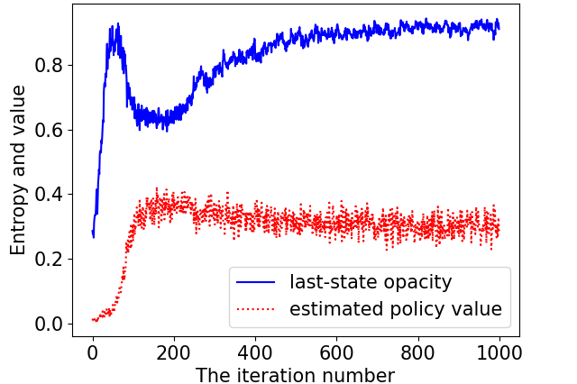
(a) Last-state opacity

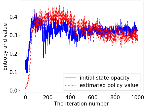
(b) Initial-state opacity

Figure 2: The result of the primal-dual policy gradient algorithm. The blue line represents the opacity and the red line represents the estimated total return.

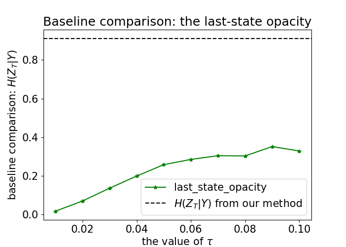
(a) Last-state opacity

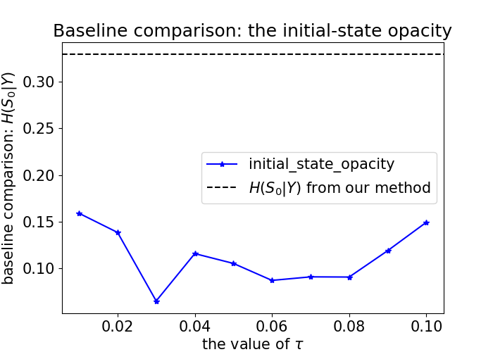
(b) Initial-state opacity

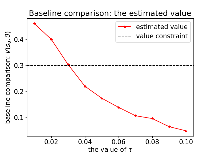
(c) Value $V(S_{0},\theta)$ of the policy

Figure 3: Comparison with baseline. The dashed lines are the entropies and values from our method. The colorful lines are entropies and values from the baseline method.

Figure 2(a) illustrates when the algorithm converges, the conditional entropy $H(Z_{T}|Y)$ eventually approaches $0.930$. The value of policy reaches $0.328$, satisfying the predefined threshold of $\delta=0.3$. Given the conditional entropy is close to 1, which is the maximal value of the entropy, the observation reveals little information regarding whether a secret location is visited, even when the observer knows the exact policy used by the robot. The conditional entropy is inversely proportional to the value/total return. This behavior is a consequence of the environmental configuration. From observing the sampled trajectories, we noticed that the agent navigates among various sensor ranges to confuse the observer, thereby diminishing the total return that P1 can achieve, as P1 is constrained from remaining stationary at the goal.

During the optimization of initial-state opacity, the set of possible initial states is four corners (cells $(0,0)$, $(0,5)$, $(5,0)$, $(5,5)$). The initial-state distribution follows a discrete uniform distribution across this set of initial states. Figure 2(b) illustrates the initial-state opacity, measured by the conditional entropy $H(S_{0}|Y)$, and the value of the policy within the primal-dual policy gradient method. The same threshold $\delta=0.3$ is employed here. When the algorithm converges, the initial conditional entropy eventually reaches $0.329$. The policy value reaches $0.301$, satisfying the predefined threshold of $\delta=0.3$. In this environment, elevated initial-state opacity indicates the observer is less uncertain about P1’s specific initial state. This result is understandable because the four sensors are highly sensitive to detect the presence of P1 in its range and different initial states give different sensor readings to the observer with high probabilities.

Since there are no other algorithms for solving the proposed opacity-enforcement planning problems, we consider a comparison with a baseline algorithm for entropy-regularized MDPs, where the objective value is a weighted sum of the total return and the discounted entropy of the policy Nachum et al. (2017). As the weight on the entropy terms increases, the policy is more stochastic and noisy.

The objective function for entropy-regularized MDPs is given by Nachum et al. (2017); Cen et al. (2022):

$$V_{\tau}(s;\theta)=V(s;\theta)+\tau H(s;\theta).$$ (27)

The discounted entropy term, $H(s;\theta)$, is defined as:

$$H(s;\theta)=-\frac{1}{1-\gamma}E_{s\sim d_{\pi_{\theta}}}\Big{[}\sum_{a\in\mathcal{A}}\pi_{\theta}(a|s)\log\pi_{\theta}(a|s)\Big{]},$$

where $d_{\pi_{\theta}}$ is the occupancy measure induced by policy $\pi_{\theta}$. The objective is to maximize the regularized total return $V_{\tau}(s;\theta)$.

We compare our method with entropy-regularized MDPs solved with different $\tau$ values, selecting $10$ values from $\tau=0.01$ to $\tau=0.1$. The following graphs (Figure 3) illustrate the results. Note that when $\tau=0.1$, the policy approaches a random policy, making it impractical to further increase opacity by raising $\tau$.

The results in Figure 3 indicate that maximizing last-state opacity and initial-state opacity cannot be achieved using standard entropy-regularized MDP. In Figure 3(a), we observed that despite the increasing value for $\tau$, the conditional entropy $H(Z_{T}|Y)$ under the baseline algorithm remains below 0.4 and below the value obtained with the proposed method, indicating that the observer has more certainty in predicting if a secret state is visited. The value of the policy decreases as $\tau$ increases, and when $\tau\geq 0.03$, the entropy-regulated policy fails to satisfy the constraint on the total return. Our method outperforms this baseline by attaining the value of $0.3$ with a last-state opacity of $0.930$. Figure 3(b) shows that the initial-state opacity fluctuates with increasing $\tau$ but does not reach the optimal initial-state opacity (0.329) achieved by our method.

These comparison experiments indicate that our proposed methods could exploit the noise in the observation to optimize opacity. This feature is not achievable using a policy computed from entropy-regularized MDPs, which do not employ the observation function.

6 Conclusion and Future Work

In this paper, we introduce information-theoretic definitions of opacity in dynamical systems modeled as Markov decision processes, against observers with imperfect information. Given the constraints on task performance, we develop opacity-enforcement policy gradient methods based on message passing in Hidden Markov Models (HMMs) for two basic types of opacity: last-state opacity and initial-state opacity. We expect the fundamental results on last-state opacity and initial-state opacity would be extended to other types of opacity, including language-based and model-based opacity and other obfuscation methods.

While the algorithm exhibits good performance in experiments, its drawback lies in high computational complexity due to the utilization of the forward-backward algorithm for gradient calculation. Finding alternative approaches to mitigate computation complexity will be among our future steps. Another direction to explore would be to investigate opacity-enforcement under different assumptions for the observer, for example, observers with imprecise knowledge about the agent’s policy. Lastly, though the objective is to maximize opacity, the same approaches can be used for minimizing opacity, and thus maximizing transparency, which is a desired property for AI and robotic systems interacting with humans. Future work would also look into potential applications and evaluate the effects of transparency in multi-agent teaming.

References

- Baum et al. [1970] Leonard E Baum, Ted Petrie, George Soules, and Norman Weiss. A maximization technique occurring in the statistical analysis of probabilistic functions of markov chains. The annals of mathematical statistics, 41(1):164–171, 1970.
- Bérard et al. [2015a] Béatrice Bérard, Krishnendu Chatterjee, and Nathalie Sznajder. Probabilistic opacity for Markov decision processes. Information Processing Letters, 115(1):52–59, January 2015.
- Bérard et al. [2015b] Béatrice Bérard, John Mullins, and Mathieu Sassolas. Quantifying opacity†. Mathematical Structures in Computer Science, 25(2):361–403, February 2015. Publisher: Cambridge University Press.
- Cen et al. [2022] Shicong Cen, Chen Cheng, Yuxin Chen, Yuting Wei, and Yuejie Chi. Fast global convergence of natural policy gradient methods with entropy regularization. Operations Research, 70(4):2563–2578, 2022.
- Dubreil et al. [2008] Jeremy Dubreil, Philippe Darondeau, and Herve Marchand. Opacity enforcing control synthesis. In 2008 9th International Workshop on Discrete Event Systems, pages 28–35, 2008.
- Guo et al. [2020] Ye Guo, Xiaoning Jiang, Chen Guo, Shouguang Wang, and Oussama Karoui. Overview of Opacity in Discrete Event Systems. IEEE Access, 8:48731–48741, 2020. Conference Name: IEEE Access.
- Han et al. [2023] X Han, Kuize Zhang, Jiahui Zhang, Zhiwu Li, and Zengqiang Chen. Strong current-state and initial-state opacity of discrete-event systems. Automatica (Oxford), 148:110756, 2023.
- Keroglou and Hadjicostis [2016] Christoforos Keroglou and Christoforos N. Hadjicostis. Probabilistic system opacity in discrete event systems. In 2016 13th International Workshop on Discrete Event Systems (WODES), pages 379–384, May 2016.
- Khouzani and Malacaria [2017] MHR. Khouzani and Pasquale Malacaria. Leakage-minimal design: Universality, limitations, and applications. In 2017 IEEE 30th Computer Security Foundations Symposium (CSF), pages 305–317, 2017.
- Lin [2011] Feng Lin. Opacity of discrete event systems and its applications. Automatica, 47(3):496–503, 2011.
- Ma et al. [2023] Haoxiang Ma, Chongyang Shi, Shuo Han, Michael R. Dorothy, and Jie Fu. Covert planning against imperfect observers, 2023.
- Marzouqi and Jarvis [2004] Mohamed Marzouqi and Ray Jarvis. Covert path planning for autonomous robot navigation. 01 2004.
- Marzouqi and Jarvis [2005] M. Marzouqi and R.A. Jarvis. Covert path planning in unknown environments with known or suspected sentry location. In 2005 IEEE/RSJ International Conference on Intelligent Robots and Systems, pages 1772–1778, 2005.
- Mazaré [2004] Laurent Mazaré. Using unification for opacity properties. 2004.
- Molloy and Nair [2023] Timothy Molloy and Girish Nair. Smoother entropy for active state trajectory estimation and obfuscation in pomdps. IEEE Transactions on Automatic Control, PP:1–16, 06 2023.
- Nachum et al. [2017] Ofir Nachum, Mohammad Norouzi, Kelvin Xu, and Dale Schuurmans. Bridging the gap between value and policy based reinforcement learning. 2017.
- Saboori and Hadjicostis [2007] Anooshiravan Saboori and Christoforos N Hadjicostis. Notions of security and opacity in discrete event systems. In 2007 46th IEEE Conference on Decision and Control, pages 5056–5061. IEEE, 2007.
- Saboori and Hadjicostis [2009] Anooshiravan Saboori and Christoforos N. Hadjicostis. Verification of k-step opacity and analysis of its complexity. In Proceedings of the 48h IEEE Conference on Decision and Control (CDC) held jointly with 2009 28th Chinese Control Conference, pages 205–210, 2009.
- Saboori and Hadjicostis [2013a] Anooshiravan Saboori and Christoforos N Hadjicostis. Current-state opacity formulations in probabilistic finite automata. IEEE Transactions on automatic control, 59(1):120–133, 2013.
- Saboori and Hadjicostis [2013b] Anooshiravan Saboori and Christoforos N. Hadjicostis. Verification of initial-state opacity in security applications of discrete event systems. Information Sciences, 246:115–132, 2013.
- Savas et al. [2020] Yagiz Savas, Melkior Ornik, Murat Cubuktepe, Mustafa O. Karabag, and Ufuk Topcu. Entropy maximization for markov decision processes under temporal logic constraints. IEEE Transactions on Automatic Control, 65(4):1552–1567, 2020.
- Shannon [1949] C. E. Shannon. Communication theory of secrecy systems. The Bell System Technical Journal, 28(4):656–715, 1949.
- Shi et al. [2023] Chongyang Shi, Abhishek N. Kulkarni, Hazhar Rahmani, and Jie Fu. Synthesis of opacity-enforcing winning strategies against colluded opponent, 2023.
- Sutton et al. [1999] Richard S Sutton, David McAllester, Satinder Singh, and Yishay Mansour. Policy gradient methods for reinforcement learning with function approximation. In S. Solla, T. Leen, and K. Müller, editors, Advances in Neural Information Processing Systems, volume 12. MIT Press, 1999.
- Watson [2011] Paul Watson. A Multi-Level Security Model for PartitioningWorkflows over Federated Clouds. In 2011 IEEE Third International Conference on Cloud Computing Technology and Science, pages 180–188, November 2011.
- Yasuoka and Terauchi [2010] H. Yasuoka and T. Terauchi. Quantitative information flow - verification hardness and possibilities. In 2010 IEEE 23rd Computer Security Foundations Symposium (CSF 2010), pages 15–27, Los Alamitos, CA, USA, jul 2010. IEEE Computer Society.
- Yin et al. [2019] Xiang Yin, Zhaojian Li, Weilin Wang, and Shaoyuan Li. Infinite-step opacity and K-step opacity of stochastic discrete-event systems. Automatica, 99:266–274, January 2019.
- Zeng and Koutny [2021] Wen Zeng and Maciej Koutny. Quantitative Analysis of Opacity in Cloud Computing Systems. IEEE Transactions on Cloud Computing, 9(3):1210–1219, July 2021.